Constructing Light Spanners Deterministically in Near-Linear Time

Abstract

Graph spanners are well-studied and widely used both in theory and practice. In a recent breakthrough, Chechik and Wulff-Nilsen [CW18] improved the state-of-the-art for light spanners by constructing a $(2k-1)(1+\varepsilon)$-spanner with $O(n^{1+\nicefrac{{1}}{{k}}})$ edges and $O_{\varepsilon}(n^{\nicefrac{{1}}{{k}}})$ lightness. Soon after, Filtser and Solomon [FS20] showed that the classic greedy spanner construction achieves the same bounds. The major drawback of the greedy spanner is its running time of $O(mn^{1+\nicefrac{{1}}{{k}}})$ (which is faster than [CW18]). This makes the construction impractical even for graphs of moderate size. Much faster spanner constructions do exist but they only achieve lightness $\Omega_{\varepsilon}(kn^{\nicefrac{{1}}{{k}}})$, even when randomization is used.

The contribution of this paper is deterministic spanner constructions that are fast, and achieve similar bounds as the state-of-the-art slower constructions. Our first result is an $O_{\varepsilon}(n^{2+\nicefrac{{1}}{{k}}+\varepsilon^{\prime}})$ time spanner construction which achieves the state-of-the-art bounds. Our second result is an $O_{\varepsilon}(m+n\log n)$ time construction of a spanner with $(2k-1)(1+\varepsilon)$ stretch, $O(\log k\cdot n^{1+\nicefrac{{1}}{{k}}})$ edges and $O_{\varepsilon}(\log k\cdot n^{\nicefrac{{1}}{{k}}})$ lightness. This is an exponential improvement in the dependence on $k$ compared to the previous result with such running time. Finally, for the important special case where $k=\log n$, for every constant $\varepsilon>0$, we provide an $O(m+n^{1+\varepsilon})$ time construction that produces an $O(\log n)$-spanner with $O(n)$ edges and $O(1)$ lightness which is asymptotically optimal. This is the first known sub-quadratic construction of such a spanner for any $k=\omega(1)$.

To achieve our constructions, we show a novel deterministic incremental approximate distance oracle. Our new oracle is crucial in our construction, as known randomized dynamic oracles require the assumption of a non-adaptive adversary. This is a strong assumption, which has seen recent attention in prolific venues. Our new oracle allows the order of the edge insertions to not be fixed in advance, which is critical as our spanner algorithm chooses which edges to insert based on the answers to distance queries. We believe our new oracle is of independent interest.

1 Introduction

A fundamental problem in graph data structures is compressing graphs such that certain metrics are preserved as well as possible. A popular way to achieve this is through graph spanners. Graph spanners are sparse subgraphs that approximately preserve pairwise shortest path distances for all vertex pairs. Formally, we say that a subgraph $H=(V,E^{\prime},w)$ of an edge-weighted undirected graph $G=(V,E,w)$ is a $t$-spanner of $G$ if for all $u,v\in V$ we have $d_{H}(u,v)\leq t\cdot d_{G}(u,v)$, where $d_{X}$ is the shortest path distance function for graph $X$ and $w$ is the edge weight function. Under such a guarantee, we say that our graph spanner $H$ has stretch $t$. In the following, we assume that the underlying graph $G$ is connected; if it is not, we can consider each connected component separately when computing a spanner.

Graph spanners originate from the 80’s [PS89, PU87] and have seen applications in e.g. synchronizers [PU87], compact routing schemes [TZ01, PU88, Che13], broadcasting [FPZW04], and distance oracles [Wul12].

The two main measures of the sparseness of a spanner $H$ is the size (number of edges) and the lightness, which is defined as the ratio $w(H)/w(MST(G))$, where $w(H)$ resp. $w(MST(G))$ is the total weight of edges in $H$ resp. a minimum spanning tree (MST) of $G$. It has been established that for any positive integer $k$, a $(2k-1)$-spanner of $O(n^{1+1/k})$ edges exists for any $n$-vertex graph [Awe85]. This stretch-size tradeoff is widely believed to be optimal due to a matching lower bound implied by Erdős’ girth conjecture [Erd64], and there are several papers concerned with constructing spanners efficiently that get as close as possible to this lower bound [TZ05, BS07, RZ11].

Obtaining spanners with small lightness (and thus total weight) is motivated by applications where edge weights denote e.g. establishing cost. The best possible total weight that can be achieved in order to ensure finite stretch is the weight of an MST, thus making the definition of lightness very natural. The size lower bound of the unweighted case provides a lower bound of $\Omega(n^{1/k})$ lightness under the girth conjecture, since $H$ must have size and weight $\Omega(n^{1+1/k})$ while the MST has size and weight $n-1$. Obtaining this lightness has been the subject of an active line of work [ADD⁺93, CDNS92, ENS15, CW18, FS20]. Throughout this paper we say that a spanner is optimal when its bounds coincide asymptotically with those of the girth conjecture. Obtaining an efficient spanner construction with optimal stretch-lightness trade-off remains one of the main open questions in the field of graph spanners.

Light spanners.

Historically, the main approach of obtaining a spanner of bounded lightness has been through different analyses of the classic greedy spanner. Given $t\geq 1$, the greedy $t$-spanner is constructed as follows: iterate through the edges in non-decreasing order of weight and add an edge $e$ to the partially constructed spanner $H$ if the shortest path distance in $H$ between the endpoints of $e$ is greater than $t$ times the weight of $e$. The study of this spanner algorithm dates back to the early 90’s with its first analysis by Althöfer et al. [ADD⁺93]. They showed that this simple procedure with stretch $2k-1$ obtains the optimal $O(n^{1+1/k})$ size, and has lightness $O(n/k)$. The algorithm was subsequently analyzed in [CDNS92, ENS15, FS20] with stretch $(1+\varepsilon)(2k-1)$ for any $0<\varepsilon<1$. Recently, a break-through result of Chechik and Wulff-Nilsen [CW18] showed that a significantly more complicated spanner construction obtains nearly optimal stretch, size and lightness giving the following theorem.

Theorem 1 ([CW18]).

Let $G=(V,E,w)$ be an edge-weighted undirected $n$-vertex graph and let $k$ be a positive integer. Then for any $0<\varepsilon<1$ there exists a $(1+\varepsilon)(2k-1)$-spanner of size $O(n^{1+1/k})$ and lightness $O_{\varepsilon}(n^{1/k})$.

Following the result of [CW18] it was shown by Filtser and Solomon [FS20] that this bound is matched by the greedy spanner. In fact, they show that the greedy spanner is existentially optimal, meaning that if there is a $t$-spanner construction achieving an upper bound $m(n,t)$ resp. $l(n,t)$ on the size resp. lightness of any $n$-vertex graph then this bound also holds for the greedy $t$-spanner. In particular, the bounds in Theorem 1 also hold for the greedy spanner.

Efficient spanners.

A major drawback of the greedy spanner is its $O(m\cdot(n^{1+1/k}+n\log n))$ construction time [ADD⁺93]. Similarly, Chechik and Wulff-Nilsen [CW18] only state their construction time to be polynomial, but since they use the greedy spanner as a subroutine, it has the same drawback. Adressing this problem, Elkin and Solomon [ES16] considered efficient construction of light spanners. They showed how to construct a spanner with stretch $(1+\varepsilon)(2k-1)$, size $O_{\varepsilon}(kn^{1+1/k})$ and lightness $O_{\varepsilon}(kn^{1/k})$ in time $O(km+\min(n\log n,m\alpha(n)))$. Improving on this, a recent paper of Elkin and Neiman [EN19] uses similar ideas to obtain stretch $(1+\varepsilon)(2k-1)$, size $O(\log k\cdot n^{1+1/k})$ and lightness $O(kn^{1/k})$ in expected time $O(m+\min(n\log n,m\alpha(n)))$.

Several papers also consider efficient constructions of sparse spanners, which are not necessarily light. Baswana and Sen [BS07] gave a $(2k-1)$-spanner with $O(kn^{1+1/k})$ edges in $O(km)$ expected time. This was later derandomized by Roditty et al. [RTZ05] (while keeping the same sparsity and running time). Recently, Miller et al. [MPVX15] presented a randomized algorithm with $O(m+n\log k)$ running time and $O(\log k\cdot n^{1+1/k})$ size at the cost of a constant factor in the stretch $O(k)$.

It is worth noting that for super-constant $k$, none of the above spanner constructions obtain the optimal $O(n^{1+1/k})$ size or $O(n^{1/k})$ lightness even if we allow $O(k)$ stretch. If we are satisfied with nearly-quadratic running time, Elkin and Solomon [ES16] gave a spanner with $(1+\varepsilon)(2k-1)$ stretch, $O_{\varepsilon}(n^{1+1/k})$ size and $O_{\varepsilon}(kn^{1/k})$ lightness in $O(kn^{2+1/k})$ time by extending a result of Roditty and Zwick [RZ11] who got a similar result but with unbounded lightness. However, this construction still has an additional factor $k$ in the lightness. Thus, the fastest known spanner construction obtaining optimal size and lightness is the classic greedy spanner – even if we allow $O(k)$ stretch or $o(kn^{1/k})$ lightness.

We would like to emphasize that the case $k=\log n$ is of special interest. This is the point on the tradeoff curve allowing spanners of linear size and constant lightness. Prior to this paper, the state of the art for efficient spanner constructions with constant lightness suffered from distortion at least $O(\log^{2}n)$. See the discussion after Corollary 1 for further details.

A summary of spanner algorithms can be seen in LABEL:tab:spanners.

Stretch Size Lightness Construction Ref $(2k-1)$ $O\left(n^{1+1/k}\right)$ $O\left(n/k\right)$ $O\left(mn^{1+1/k}\right)$ [ADD⁺93]^∗ $(2k-1)(1+\varepsilon)$ $O\left(n^{1+1/k}\right)$ $O\left(kn^{1/k}\right)$ $O\left(mn^{1+1/k}\right)$ [CDNS92]^∗ $(2k-1)$ $O(n^{1+1/k})$ $\Omega(W)\text{ }^{**}$ $O\left(kn^{2+1/k}\right)$ [RZ11] $(2k-1)$ $O\left(kn^{1+1/k}\right)$ $\Omega\left(n^{1+1/k}\right)\text{ }^{**}$ $O\left(kmn^{1/k}\right)$ [TZ05]^# $(2k-1)(1+\varepsilon)$ $O\left(n^{1+1/k}\right)$ $O\left(kn^{1/k}\right)$ $O\left(kn^{2+1/k}\right)$ [ES16] $(2k-1)(1+\varepsilon)$ $O\left(n^{1+1/k}\right)$ $O\left(n^{1/k}\cdot k/\log k\right)$ $O\left(mn^{1+1/k}\right)$ [ENS15]^∗ $(2k-1)(1+\varepsilon)$ $O\left(n^{1+1/k}\right)$ $O\left(n^{1/k}\right)$ $n^{\Theta(1)}$ [CW18] $(2k-1)(1+\varepsilon)$ $O\left(n^{1+1/k}\right)$ $O\left(n^{1/k}\right)$ $O\left(mn^{1+1/k}\right)$ [FS20]^∗ $(2k-1)$ $O\left(kn^{1+1/k}\right)$ $\Omega(W)\text{ }^{**}$ $O\left(km\right)$ [BS07, RTZ05] $(2k-1)(1+\varepsilon)$ $O\left(kn^{1+1/k}\right)$ $O\left(kn^{1/k}\right)$ $O\left(km+n\log n\right)$ [ES16] $O(k)$ $O(\log k\cdot n^{1+1/k})$ $\Omega(W)$ $O(m+n\cdot\log k)$ [MPVX15]^# $(2k-1)(1+\varepsilon)$ $O(\log k\cdot n^{1+1/k})$ $O\left(k\cdot n^{1/k}\right)$ $O(m+n\cdot\log n)$ [EN19]^# $(2k-1)(1+\varepsilon)$ $O\left(\log k\cdot n^{1+1/k}\right)$ $\Omega(W)$ $O(m+n\log k\log^{(s)}k)$ Theorem 6 $(2k-1)(1+\varepsilon)$ $O\left(\log k\cdot n^{1+1/k}\right)$ $O\left(\log k\cdot n^{1/k}\right)$ $O(m+n\cdot\log n)$ Theorem 3 $(2k-1)(1+\varepsilon)$ $O\left(n^{1+1/k}\right)$ $O\left(n^{1/k}\right)$ $O(n^{2+1/k+\varepsilon^{\prime}})$ Theorem 2 $O(k)$ $O\left(n^{1+1/k}\right)$ $O\left(n^{1/k}\right)$ $O\left(m+n^{1+\varepsilon^{\prime}+1/k}\right)$ Theorem 4 $O(\log n)/\delta$ $O\left(n\right)$ $1+\delta$ $O\left(m+n^{1+\varepsilon^{\prime}}\right)$ Corollary 1

Table 1: Table of related spanner constructions. In the top of the table we list non-efficient spanner constructions. In the middle we list known efficient spanner constructions. In the bottom we list our contributions. Results marked ^∗ are different analyses of the greedy spanner. Results marked ^# are randomized. Lightness complexities marked ^∗∗ are from the analysis in Section 9 and $W$ denotes the maximum edge weight of the input graph. The bounds hold for any constant $\varepsilon,\varepsilon^{\prime}>0$.

table]tab:spanners

1.1 Our results

We present the first spanner obtaining the same near-optimal guarantees as the greedy spanner in significantly faster time by obtaining a $(1+\varepsilon)(2k-1)$ spanner with optimal size and lightness in $O_{\varepsilon}(n^{2+1/k+\varepsilon^{\prime}})$ time. We also present a variant of this spanner, improving the running time to $O(m+n\log n)$ by paying a $\log k$ factor in the size and lightness. Finally, we present an optimal $O_{\varepsilon}(\log n)$-spanner which can be constructed in $O(m+n^{1+\varepsilon})$ time. This special case is of particular interest in the literature (see e.g. [BFN19, KX16]). Furthermore, all of our constructions are deterministic, giving the first subquadratic deterministic construction without the additional dependence on $k$ in the size of the spanner. As an important tool, we introduce a new deterministic approximate incremental distance oracle which works in near-linear time for maintaining small distances approximately. We believe this result is of independent interest.

More precisely, we show the following theorems.

Theorem 2.

Given a weighted undirected graph $G=(V,E,w)$ with $m$ edges and $n$ vertices, any positive integer $k$, and $\varepsilon,\varepsilon^{\prime}>0$ where $\varepsilon$ arbitrarily close to $0$ and $\varepsilon^{\prime}$ is a constant, one can deterministically construct an $(1+\varepsilon)(2k-1)$-spanner of $G$ with $O_{\varepsilon}(n^{1+1/k})$ edges and lightness $O_{\varepsilon}(n^{1/k})$ in $O(n^{2+1/k+\varepsilon^{\prime}})$ time.

Theorem 3.

Given a weighted undirected graph $G=(V,E,w)$ with $m$ edges and $n$ vertices, a positive integer $k\geq 640$, and $\epsilon>0$, one can deterministically construct a $(2k-1)(1+\varepsilon)$-spanner of $G$ with $O_{\varepsilon}(\log k\cdot n^{1+1/k})$ edges and lightness $O_{\varepsilon}\left(\log k\cdot n^{1/k}\right)$ in time $O\left(m+n\log n\right)$.

Note that in Theorem 3 we require $k$ to be larger than $640$. This is not a significant limitation, as for $k=O(1)$ [ES16] is already optimal.

Our $O(\log n)$-spanner is obtained as a corollary of the following more general result.

Theorem 4.

Given a weighted undirected graph $G=(V,E,w)$ with $m$ edges and $n$ vertices, any positive integer $k$ and constant $\varepsilon^{\prime}>0$, one can deterministically construct an $O(k)$-spanner of $G$ with $O(n^{1+1/k})$ edges and lightness $O(n^{1/k})$ in $O(m+n^{1+\varepsilon^{\prime}+1/k})$ time.

We note that the stretch $O(k)$ of Theorem 4 (and Corollary 1 below) hides an exponential factor in $1/\varepsilon^{\prime}$, thus we only note the result for constant $\varepsilon^{\prime}$. Bartal et. al. [BFN19] showed that given a spanner construction that for every $n$-vertex weighted graph produces a $t(n)$-stretch spanner with $m(n,t)$ edge and $l(n,t)$ lightness in $T(n,m)$ time, then for every parameter $0<\delta<1$ and every graph $G$, one can construct a $t/\delta$-spanner with $m(n,t)$ edges and $1+\delta\cdot l(n,t)$ lightness in $T(n,m)+O(m)$ time. Plugging $k=\log n$ and using this reduction w.r.t. $\delta$ in Theorem 4, and $\delta^{\prime}=\frac{\delta}{\log\log n}$ in Theorem 3, we get

Corollary 1.

Let $G=(V,E,w)$ be a weighted undirected $n$-vertex graph, let $\varepsilon^{\prime}>0$ be a constant and $\delta>0$ be a parameter arbitrarily close to $0$. Then one can construct a spanner of $G$ with:

1. $O(\log n)/\delta$ stretch, $O(n)$ edges and $1+\delta$ lightness in time $O(m+n^{1+\varepsilon^{\prime}})$.

2. $O(\log n\log\log n)/\delta$ stretch, $O(n\log\log n)$ edges and $1+\delta$ lightness in time $O(m+n\log n)$.

Corollary 1 above should be compared to previous attempts to efficiently construct a spanner with constant lightness. Although not stated explicitly, the state-of-the-art algorithms of [ES16, EN19], combined with the lemma from [BFN19], provide an efficient spanner construction with $1+\delta$ lightness, $O(n\log\log n)$ edges and only $O(\log^{2}n/\delta)$ stretch.

We emphasize, that Corollary 1 is the first sub-quadratic construction of spanner with optimal size and lightness for any non-constant $k$.

In order to obtain Theorem 4 we construct the following deterministic incremental approximate distance oracle with near-linear total update time for maintaining small distances. We believe this result is of independent interest, and discuss it in more detail in the related work section below and in Section 3.

Theorem 5.

Let $G$ be a graph that undergoes a sequence of $m$ edge insertions. For any constant $\varepsilon^{\prime}>0$ and parameter $d\geq 1$ there exists a data structure which processes the $m$ insertions in total time $O(m^{1+\varepsilon^{\prime}}\cdot d)$ and can answer queries at any point in the sequence of the following form. Given a pair of nodes $u,v$, the oracle gives, in $O(1)$ time, an estimate $\hat{d}(u,v)$ such that $\hat{d}(u,v)\geq d(u,v)$ and if $d(u,v)\leq d$ then $\hat{d}(u,v)=O(1)\cdot d(u,v)$.

Theorem 5 assumes that $\varepsilon^{\prime}$ is constant; the $O$-notation hides a factor exponential in $1/\varepsilon^{\prime}$ for both total update time and stretch whereas the query time bound only hides a factor of $1/\varepsilon^{\prime}$.

We also obtain the following sparse, but not necessarily light, spanner in linear time as a subroutine in proving Theorem 3.

Theorem 6.

Given a weighted undirected graph $G=(V,E,w)$ with $m$ edges and $n$ vertices, any positive integer $k$, any $\epsilon>0$, and any positive integer $s=O(1)$, one can deterministically construct a $(2k-1)(1+\varepsilon)$-spanner of $G$ with $O_{\varepsilon}(n^{1+1/k}\cdot\log k)$ edges; the running time is $O(m+n\log^{(s-1)}k\log k)$ and if $k\leq\log n/\log^{(s+1)}n$, the running time is $O(m)$.

Here, the function $\log^{(s)}$ is $\log$ concatenated with itself $s$ times. Specifically, $\log^{(0)}n=n$, $\log^{(1)}n=\log n$, and in general for $s\geq 1$, $\log^{(s)}n=\log(\log^{(s-1)}n)$. $\log^{*}n$ is the minimum index $s$ such that $\log^{(s)}n\leq 2$.

Note that since we may assume that $k=O(\log n)$, the time bound of Theorem 6 is linear for almost all choices of $k$ and very close to linear for any choice of $k$.

Organization

In Section 4 we state our framework that used in Theorems 4, 3 and 2. Theorem 4 is proved in Section 5, and Theorem 2 in Section 5.2. Theorem 3 is proved in Section 6. Theorem 5 is proved in Section 8. The proof of Theorem 6 appears in Section 7.

1.2 Related work

Closely related to graph spanners are approximate distance oracles (ADOs). An ADO is a data structure which, after preprocessing a graph $G$, is able to answer distance queries approximately. Distance oracles are studied extensively in the literature (see e.g. [TZ05, Wul13, Che14, Che15]) and often use spanners as a building block. The state of the art static distance oracle is due to Chechik [Che15], where a construction of space $O(n^{1+1/k})$, stretch $2k-1$, and query time $O(1)$ is given. Our distance oracle of Theorem 5 should be compared to the result of Henzinger, et al. [HKN16], who gave a deterministic construction for incremental (or decremental) graphs with a total update time of $O_{\varepsilon}(mn\log n)$, a query time of $O(\log\log n)$ and stretch $1+\varepsilon$. For our particular application, we require near-linear total update time and only good stretch for short distances, which are commonly the most troublesome when constructing spanners. It should be added that Henzinger et al. give a general deterministic data structure for choosing centers, i.e., vertices which are roots of shortest path trees maintained by the data structure. While this data structure may be fast when the total number of centers is small, we need roughly $n$ centers and it is not clear how this number can be reduced. Having this many centers requires at least order $mn$ time with their data structure.

To achieve our fast update time bound, we are interested in trading worse stretch for distances above parameter $d$ for construction time. Roditty and Zwick [RZ12] gave a randomized distance oracle for this case, however their construction does not work against an adaptive adversary as is required for our application, where the edges to be inserted are determined by the output to the queries of the oracle (see Section 3 for more discussion on this). Removing the assumption of a non-adaptive adversary in dynamic graph algorithms has seen recent attention at prestigious venues, e.g. [Wul17, BHN16]. Our new incremental approximate distance oracle for short distances given in Theorem 5 is deterministic and thus is robust against such an adversary, and we believe it may be of independent interest as a building block in deterministic dynamic graph algorithms.

For unweighted graphs, there is a folklore spanner construction by Halperin and Zwick [HZ96] which is optimal on all parameters. The construction time is $O(m)$, it has $O(n^{1+1/k})$ edges and $2k-1$ stretch. In Section 6 we will use this spanner as a building block in proving Theorem 3.

2 Preliminaries

Consider a weighted graph $G=(V,E,w)$, we will abuse notation and refer to as $E$ both a set of edges and the graph itself. $d_{G}$ will denote the shortest path metric (that is $d_{G}(v,u)$ is the weight of the lightest path between $v,u$ in $G$. Given a subset $V^{\prime}$ of $V$, $G[V^{\prime}]$ is the induced graph by $V^{\prime}$. That is it has $V^{\prime}$ as it vertices, $E\cap{V^{\prime}\choose 2}$ as its edges and $w$ as weight function. The diameter of a vertex set $V^{\prime}$ in a graph $G^{\prime}$ ${\rm diam}_{G^{\prime}}(V^{\prime})=\max_{u,v\in V^{\prime}}d_{G^{\prime}}(u,v)$ is the maximal distance between two vertices in $V^{\prime}$ under the shortest path metric induced by $G^{\prime}$. For a set of edges $A$ with weight function $w$, the aspect ratio of $A$ is $\max_{e\in A}w(e)/\min_{e\in A}w(e)$. The sparsity of $A$ is simply $|A|$ its size.

We will assume that $k=O(\log n)$ as the guarantee for lightness and sparsity will not be improved by picking larger $k$. Instead of proving $(1+\varepsilon)(2k-1)$ bound on stretch, we will prove only $(1+O(\varepsilon))(2k-1)$ bound. This is good enough, as Post factum we can scale $\varepsilon$ accordingly. By $O_{\varepsilon}$ we denote asymptotic notation which hides polynomial factors of $1/\varepsilon$, that is $O_{\varepsilon}(f)=O(f)\cdot{\rm poly}(\frac{1}{\varepsilon})$.

3 Paper overview

General framework

Theorems 2, 4 and 3 are generated via a general framework. The framework is fed two algorithms for spanner constructions: $A_{1}$, an algorithm suitable for graphs with small aspect ratio, and $A_{2}$, an algorithm that returns a sparse spanner, but with potentially unbounded lightness. We consider a partition of the edges into groups according to their weights. For treating most of the groups we use exponentially growing clusters, partitioning the edges according to weight. Each such group has bounded aspect ratio, and thus we can use $A_{1}$. Due to the exponential growth rate, we show that the contribution of all the different groups is converging. Thus only the first group is significant. However, with this approach we need a special treatment for edges of small weight. This is, as using the previous approach, the number of clusters needed to treat light edges is unbounded. Nevertheless, these edges have small impact on the lightness and we may thus use algorithm $A_{2}$, which ignores this property.

The main work in proving Theorems 2, 4 and 3 is in designing the algorithms $A_{1}$ and $A_{2}$ described briefly below.

Approximate greedy spanner

The major time consuming ingredient of the greedy spanner algorithm is its shortest path computations. By instead considering approximate shortest path computations we significantly speed this process up. We are the first to apply this idea on general graphs, while it has previously been applied by [DN97, FS20] on particular graph families. Specifically, we consider the following algorithm: given some parameters $t<t^{\prime}$, initialize $H\leftarrow\emptyset$ and consider the edges $(u,v)\in E$ according to increasing order of weight. If $d_{H}(u,v)>t^{\prime}\cdot w(u,v)$ the algorithm is obliged to add $(u,v)$ to $H$. If $d_{H}(u,v)<t\cdot w(u,v)$, the algorithm is forbidden to add $(u,v)$ to $H$. Otherwise, the algorithm is free to include the edge or not. As a result, we will get spanner with stretch $t^{\prime}$, which has the same lightness and sparsity guarantees of the greedy $t$-spanner. Note however, that the resulting spanner is not necessarily a subgraph of any greedy spanner.

We obtain both Theorem 2 and Theorem 4 using this approach via an incremental approximate distance oracle. It is important to note that the edges inserted into $H$ using this approach depend on the answers to the distance queries. It is therefore not possible to use approaches that do not work against an adaptive adversary such as the result of Roditty and Zwick [RZ12], which is based on random sampling. Furthermore, this is the case even if we allow the spanner construction itself to be randomized. In order to obtain Theorem 2, we use our previously described framework coupled with the “approximately greedy spanner” using an incremental $(1+\varepsilon)$-approximate distance oracle of Henzinger et al. [HKN16]. For Theorem 4, we present a novel incremental approximate distance oracle, which is described below. This is the main technical part of the paper and we believe that it may be of independent interest.

Deterministic distance oracle

The main technical contribution of the paper and key ingredient in proving Theorem 4 is our new deterministic incremental approximate distance oracle of Theorem 5. The oracle supports approximate distance queries of pairs within some distance threshold, $d$. In particular, we may set $d$ to be some function of the stretch of the spanner in Theorem 4. Similar to previous work on distance oracles, we have some parameter, $k$, and maintain $k$ sets of nodes $\emptyset=A_{k-1}\subseteq\ldots\subseteq A_{0}=V$, and for each $u\in A_{i}$ we maintain a ball of radius $r\leq d_{i}$. Here, $d_{i}$ is a distance threshold depending on the parameter $d$ and which set $A_{i}$ we are considering, and $r$ is chosen such that the total degree of nodes in the ball of radius $r$ from $u$ is relatively small. The implementation of each ball can be thought of as an incremental Even-Shiloach tree. The set $A_{i+1}$ is then chosen as a maximal set of nodes with disjoint balls (see Figure 3 in Section 8.1). Here we use the fact that the vertices in $A_{i+1}$ are centers of disjoint balls in $A_{i}$ to argue that $A_{i+1}$ is much smaller than $A_{i}$. The decrease in size of $A_{i+1}$ pays for an increase in the maximum ball radius $d_{i}$ at each level. The ball of a node $u$ may grow in size during edge insertions. In this case, we freeze the ball associated with $u$, shrink the radius $r$ associated with $u$, and create a new ball with the new radius. Thus, for each $A_{i}$ we end up with $O(\log d)$ different radii for which we pick a maximal set of nodes with disjoint balls. For each node $u_{i}\in A_{i}$ we may then associate a node $u_{i+1}\in A_{i+1}$ whose ball intersects with $u_{i}$’s. We use these associated nodes in the query to ensure that the path distance we find is not “too far away” from the actual shortest path distance. Consider a query pair $(u,v)$. Then the query algorithm iteratively finds a sequence of vertices $u=u_{0}\in A_{0},u_{1}\in A_{1},...,u_{i}\in A_{i}$; $d_{i}$ is picked such that if $v$ is not in the ball centered at $u_{i}$ with radius $d_{i}$ then the shortest path distance between $u$ and $v$ is at least $d$ and the algorithm outputs $\infty$. Otherwise, the algorithm uses the shortest path distances stored in the balls that it encounters to output the weight of a $uv$-path $(u=u_{0})\leadsto u_{1}\leadsto\ldots\leadsto u_{i}\leadsto v$ as an approximation of the shortest path distance between $u$ and $v$.

Almost linear spanner

Chechik and Wulff-Nilsen [CW18] implicitly used our general framework, but used the (time consuming) greedy spanner both as their $A_{2}$ component and as a sub-routine in $A_{1}$. We show an efficient alternative to the algorithm of [CW18]. For the $A_{2}$ component we provide a novel sparse spanner construction (Theorem 6, see paragraph below). For $A_{1}$, we perform a hierarchical clustering, while avoiding the costly exact diameter computations used in [CW18]. Finally, we replace the greedy spanner used as a sub-routine of [CW18] by an efficient spanner that exploits bounded aspect ratio (see Lemma 5). This spanner can be seen as a careful adaptation of Elkin and Solomon [ES16] analyzed in the case of bounded aspect ratio. The idea here is (again) a hierarchical partitioning of the vertices into clusters of exponentially increasing size. However, here the growth rate is only $(1+\varepsilon)$. Upon each clustering we construct a super graph with clusters as vertices and graph edges from the corresponding weight scale as inter-cluster edges. To decide which edges in each scale add to our spanner, we execute the extremely efficient spanner of Halperin and Zwick [HZ96] for unweighted graphs.

Linear time sparse spanner

As mentioned above we provide a novel sparse spanner construction as a building block in proving Theorem 3. Our construction is based on partitioning edges into $O_{\varepsilon}(\log k)$ “well separated” sets $E_{1},E_{2},\ldots$, such that the ratio between $w(e)$ and $w(e^{\prime})$ for edges $e,e^{\prime}\in E_{i}$ is either a constant or at least $k$. This idea was previously employed by Elkin and Neiman [EN19] based on [MPVX15]. For these well-separated graphs, Elkin and Neiman used an involved clustering scheme based on growing clusters according to exponential distribution, and showed that the expected number of inter-cluster edges, in all levels combined, is small enough. We provide a linear time deterministic algorithm with an arguably simpler clustering scheme. Our clustering is based upon the clusters defined implicitly by the spanner for unweighted graphs of Halperin and Zwick [HZ96]. In particular, we introduce a charging scheme, such that each edge added to our spanner is either paid for by a large cluster with many coins, or significantly contributing to reduce the number of clusters in the following level.

4 A framework for creating light spanners efficiently

In this section we describe a general framework for creating spanners, which we will use to prove our main results. The framework is inspired by a standard clustering approach (see e.g. [ES16] and [CW18]). The spanner framework takes as input two spanner algorithms for restricted graph classes, $A_{1}$ and $A_{2}$, and produces a spanner algorithm for general graphs. The algorithm $A_{1}$ works for graphs with unit weight MST edges and small aspect ratio, and $A_{2}$ creates a small spanner with no guarantee for the lightness. The main work in showing Theorems 2, 3, and 4 is to construct the algorithms, $A_{1}$ and $A_{2}$, that go into Lemma 1 below. We do this in Sections 5 and 6. The framework is described in the following lemma.

Lemma 1.

Let $G=(V,E)$ be a weighted graph with $n$ nodes and $m$ edges and let $k>0$ be an integer, $g>1$ a fixed parameters and $\varepsilon>0$. Assume that we are given two spanner construction algorithms $A_{1}$ and $A_{2}$ with the following properties:

• $A_{1}$ computes a spanner of stretch $f_{1}(k)$, size $O_{\varepsilon}(s_{1}(k)\cdot n^{1+1/k})$ and lightness $O_{\varepsilon}(l_{1}(k)\cdot n^{1/k})$ in time $T_{1}(n,m,k)$ when given a graph with maximum weight $g^{k}$, where all MST edges have weight $1$. Moreover, $T_{1}$ has the property that $\sum_{i=0}^{\infty}T_{1}\!\left(\frac{n}{g^{ik}},m_{i},k\right)=O\left(T_{1}\!\left(n,m,k\right)\right)$, where $\sum_{i}m_{i}=m+O(n)$.

• $A_{2}$ computes a spanner of stretch $f_{2}(k)$ and size $O_{\varepsilon}(s_{2}(k)\cdot n^{1+1/k})$ in time $T_{2}(n,m,k)$.

Then one can compute a spanner of stretch $\max((1+\varepsilon)f_{1}(k),f_{2}(k))$, size $O_{\varepsilon}((s_{1}(k)+s_{2}(k))n^{1+1/k})$, and lightness $O_{\varepsilon}((l_{1}(k)+s_{2}(k))\cdot n^{1/k})$ in time $O(T_{1}(n,m,k)+T_{2}(n,m,k)+m+n\log n)$.

As an example, let us assume that we have both an optimal spanner algorithm for graphs with small aspect ratio, and an optimal spanner algorithm for sparse spanners in weighted graph. Specifically, we have algorithm $A_{1}$ that given a graph as above creates a $(1+\varepsilon)(2k-1)$-spanner with $O_{\varepsilon}(n^{1+1/k})$ edges and lightness $O_{\varepsilon}(n^{1/k})$ in $O_{\varepsilon}(m+n\log n)$ time. In addition we have algorithm $A_{2}$ that returns an $(1+\varepsilon)(2k-1)$-spanner with $O_{\varepsilon}(n^{1+1/k})$ edges in $O_{\varepsilon}(m)$ time. Then, given a general graph, Lemma 1 provide us with a $(1+\varepsilon)(2k-1)$-spanner of $O_{\varepsilon}(n^{1+1/k})$ size and $O_{\varepsilon}(n^{1/k})$ lightness, in time $O_{\varepsilon}(m+n\log n)$.

Before proving Lemma 1 we need to describe the clustering approach. The main tool needed is what we call an $(i,\varepsilon)$-clustering. This clustering procedure is performed on graphs where all the MST edges have unit weight. Let $G,g,\varepsilon,k$ be as in Lemma 1, then we say that an $(i,\varepsilon)$-clustering is a partitioning of $V$ into clusters $C_{1},\ldots,C_{n_{i}}$, such that each $C_{j}$ contains at least $\varepsilon g^{ik}$ nodes and has diameter at most $4\varepsilon g^{ik}$ (even when restricted to MST edges of $G$). Let $G_{i}$ denote the graph obtained by contracting the clusters of such an $(i,\varepsilon)$-clustering of $G$, and keeping the MST edges only. Then $G_{i}$ has $n_{i}$ nodes, and we can construct $G_{i}$ from $G_{i-1}$ as follows. Start at some vertex $v$ in $G_{i-1}$ (corresponding to an $(i-1,\varepsilon)$-cluster) and iteratively grow an $(i,\varepsilon)$-cluster $\varphi_{v}$ by joining arbitrary un-clustered neighbors to $\varphi_{v}$ in $G_{i-1}$ one at a time. If the number of original vertices in $\varphi_{v}$ reaches $\varepsilon g^{ik}$, make $\varphi_{v}$ into an $(i,\varepsilon)$-cluster, where the current vertices in $\varphi_{v}$ are called its core. We argue that the diameter of the core is bounded by $\varepsilon g^{ik}+4\varepsilon g^{(i-1)k}$. If the vertex $v$ (from $G_{i}$) already contains $\varepsilon g^{ik}$ vertices, then $\varphi_{v}=v$ and by the induction hypothesis the diameter of $\varphi_{v}$ is at most $4\varepsilon g^{(i-1)k}$. Otherwise ($|v|<\varepsilon g^{ik}$), consider the last vertex $u\in G_{i-1}$ to join $\varphi_{v}$. As $u$ joins $\varphi_{v}$, necessarily $|\varphi_{v}\setminus u|<\varepsilon g^{ik}$. In particular, the diameter of $\varphi_{v}\setminus u$ (restricted to MST edges) is at most $g^{ik}-1$. The diameter of $u$ is at most $4\varepsilon g^{(i-1)k}$ and therefore the diameter of $\varphi_{v}$ is indeed bounded by $\varepsilon g^{ik}+4\varepsilon g^{(i-1)k}$.

We perform this procedure starting at an un-clustered vertex until all vertices of $G_{i-1}$ belong to some $(i,\varepsilon)$-cluster. In the case where $\varphi_{v}$ has no un-clustered neighbors, but does not contain $\varepsilon g^{ik}$ vertices, we simply merge it with an existing $(i,\varepsilon)$-cluster $\varphi_{u}$ via an MST-edge to the core of $\varphi_{u}$. Note that the size of $\varphi_{v}$, and therefore its diameter, before the merging is at most $\varepsilon g^{ik}-1$ (as each cluster is connected when restricting to MST edges). To show that this gives a valid $(i,\varepsilon)$-clustering, consider an $(i,\varepsilon)$-cluster $\varphi_{v}$ with core $\tilde{\varphi}_{v}$. Suppose that the “sub-clusters” $\tilde{\varphi}_{u_{1}},\dots,\tilde{\varphi}_{u_{s}}$ were merged into $\tilde{\varphi}_{v}$ during this process. The diameter of $\varphi_{v}$ is then bounded by

$${\rm diam}(\tilde{\varphi}_{v})+2+\max_{j,j^{\prime}}({\rm diam}(\tilde{\varphi}_{u_{j}})+{\rm diam}(\tilde{\varphi}_{u_{j^{\prime}}}))\leq(\varepsilon g^{ik}+4\varepsilon g^{(i-1)k})+2\varepsilon g^{ik}\leq 4\varepsilon g^{ik}\leavevmode\nobreak\ .$$

Moreover, the size of $\varphi_{v}$ is at least the size of its core, $|\tilde{\varphi}_{v}|\geq\varepsilon g^{ik}$. See figure Figure 1 for illustration.

Figure 1: The small cycles represent $(i-1,\varepsilon)$-clusters, which are the vertices of $G_{i-1}$. The $(i-1,\varepsilon)$-cluster $v$ iteratively grows a cluster around itself until it contains $\varepsilon g^{ik}$ original vertices. This current cluster is called $\tilde{\varphi}_{v}$. $\tilde{\varphi}_{v}$ also called the core of $\varphi_{v}$, an $(i,\varepsilon)$-cluster that we will have at the end of the process. Afterwards, the $(i-1,\varepsilon)$-cluster $u_{1}$ iteratively grow a cluster around itself. When the temporary cluster is $\tilde{\varphi}_{u_{1}}$ there are no outgoing edges to unclustered vertices. However, since $G_{i-1}$ is connected, there is some outgoing edge. Necessarily the second endpoint of this edge belongs to the core of an existing cluster (here, $\tilde{\varphi}_{v}$), that is, as $\tilde{\varphi}_{v}$ stop growing while still having unclustered neighbors. All the vertices of $\tilde{\varphi}_{u_{1}}$ joins the cluster of $v$. In a similar manner, $\tilde{\varphi}_{u_{2}}$ and $\tilde{\varphi}_{u_{3}}$ are also joined into the cluster of $v$. In the end of the algorithm, the $(i,\varepsilon)$-cluster of $v$ is $\varphi_{v}=\tilde{\varphi}_{v}\cup\tilde{\varphi}_{u_{1}}\cup\tilde{\varphi}_{u_{2}}\cup\tilde{\varphi}_{u_{3}}$.

 

Note that we have $n_{i}\leq\frac{n}{\varepsilon g^{ik}}$. Using the above procedure, we can construct the $(i+1,\varepsilon)$ clustering from the $(i,\varepsilon)$ clustering in $O(n_{i})$ time. Therefore we can construct the clusters for all the levels in $O\left(\sum_{i\geq 0}n_{i}\right)=O\left(n\sum_{i\geq 0}\frac{1}{g^{ik}}\right)=O(n)$ time (if we are given the MST).

With this tool in hand, we may now prove Lemma 1.

Proof of Lemma 1.

The proof constructs an algorithm consisting of two phases. The preparation phase where $A_{2}$ is used to reduce the problem to a graph where all MST edges have weight $1$, and the bootstrapping phase where we perform an iterative clustering of the graph to obtain several graphs with small aspect-ratio, where we can apply $A_{1}$.

Preparation phase: Let $T$ be an MST of $G$ and let $w^{\prime}=\sum_{(u,v)\in T}\frac{w(u,v)}{n-1}$. Define $G_{2}$ to be $G$ with all edges of weight greater than $w^{\prime}/\varepsilon$ removed and let $H^{2}$ be the spanner resulting from running $A_{2}$ on $G_{2}$. Next, we construct $G_{1}$ from $G$ as follows. First, round up the weight of each edge in $G$ to the nearest multiple of $w^{\prime}$. For each edge $e\in T$ subdivide it such that each edge of the resulting MST has weight $w^{\prime}$ . As the weight of each edge increase by at most an additive factor of $w^{\prime}$, the weight of the MST increase by at most $(n-1)w^{\prime}\leq w(T)$. The new number of vertices is bounded by $\sum_{(u,v)\in T}\left\lceil\frac{w(u,v)}{w^{\prime}}\right\rceil\leq(n-1)+\frac{1}{w^{\prime}}\cdot\sum_{(u,v)\in T}w(u,v)<2n$. Finally, divide the weight of each edge by $w^{\prime}$. This finishes the construction of $G_{1}$.

Bootstrapping phase: We will now use $A_{1}$ to make a spanner $H^{1}$ for the graph $G_{1}$ created above. We start by partitioning the edges into sets $E_{i}$, where $E_{i}$ contains all edges of $G_{1}$ with weights in $[g^{ik},g^{(i+1)k})$. Note that since each MST edge of $G_{1}$ has weight $1$ we only need to consider edges with weight up to $O(n)$. Next, we let $T$ be an MST of $G_{1}$ and for all $i=0,1,\ldots,O(\log n)$ we create $T_{i}$ by contracting all clusters of an $(i,\varepsilon)$-clustering of $T$, where the $(i,\varepsilon)$-clustering is computed as described above. Note that $T_{i}$ is also a tree since each cluster is a connected subtree of $T$. We now construct graphs $G_{i}$ by taking $T_{i}$ and adding any minimum weight edge of $E_{i}$ going between each pair of clusters (i.e. nodes corresponding to clusters). Finally, we divide the weight of each non-MST edge of $G_{i}$ by $g^{ik}$. This gives us a graph with maximum weight $g^{k}$, where MST edges have weight $1$. We call this new weight function $w_{i}$. Let $H_{i}$ be the spanner obtained by running algorithm $A_{1}$ on $G_{i}$. Finally, let $H^{1}$ be the union of all $H_{i}$s, where each edge of $H_{i}$ is replaced by the corresponding edge(s) from $G$.

Analysis: We set the final spanner $H=MST(G)\cup H^{1}\cup H^{2}$. To bound the stretch of $H$ first note that any edge of $G_{2}$ has stretch at most $f_{2}(k)$ from $H^{2}$. What remains is to bound the stretch of non-MST edges $(u,v)$ with $w(u,v)\geq w^{\prime}/\varepsilon$. First, observe that the rounding procedure used to create $G_{1}$ can at most increase the weight of $(u,v)$ in $G_{1}$ by a factor of $(1+\varepsilon)$ compared to $G$.

Now assume that $(u,v)\in E_{i}$ for some $i$. Let $\varphi_{u}$ and $\varphi_{v}$ denote the clusters containing $u$, respectively, $v$ in $G_{i}$. If $\varphi_{u}=\varphi_{v}$ we know that the distance between $u$ and $v$ using the MST is at most $4\varepsilon g^{ik}$ and we are done. Thus, assume that $\varphi_{u}\neq\varphi_{v}$. By definition of $G_{i}$, there must be some edge $(\varphi_{u},\varphi_{v})$ in $G_{i}$ with $w_{i}(\varphi_{u},\varphi_{v})\leq(1+\varepsilon)\cdot w(u,v)/g^{ik}$. We know that there is a path $\{\varphi_{u}=\varphi_{z_{0}}\varphi_{z_{1}}\dots\varphi_{z_{s}}=\varphi_{v}\}$ from $\varphi_{u}$ to $\varphi_{v}$ in $H_{i}$ of length at most $f_{1}(k)\cdot w_{i}(\varphi_{u},\varphi_{v})$. Recall that the minimum weight in $H_{i}$ is $1$, thus we have $s\leq f_{1}(k)\cdot w_{i}(\varphi_{u},\varphi_{v})$. Furthermore, the diameter of each cluster, $\varphi_{z_{q}}$, is at most $4\varepsilon g^{ik}$. We now conclude (see Figure 2 for illustration)

$$d_{H}(u,v) \leq\sum_{q=0}^{s}{\rm diam}_{T}(\varphi_{z_{q}})+g^{ik}\sum_{q=0}^{s-1}w_{i}(\varphi_{z_{q}},\varphi_{z_{q+1}})$$

$$\leq(s+1)\cdot 4\varepsilon g^{ik}+g^{ik}f_{1}(k)\cdot w_{i}(\varphi_{u},\varphi_{v})$$

$$\leq(1+8\varepsilon)\cdot g^{ik}\cdot f_{1}(k)\cdot w_{i}(\varphi_{u},\varphi_{v})$$

$$\leq(1+O(\varepsilon))\cdot f_{1}(k)\cdot w(u,v)$$ (1)

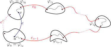
Figure 2: $e=(u,v)$ is an edge (colored in blue) in $E_{i}$, such that $u$ and $v$ belong to the $i$-clusters $\varphi_{u},\varphi_{v}$, respectively. The closed bold black curves represent $i$-clusters. The red edges represent edges in $H_{i}$. The thin black curves represent MST paths. There is an edge $e^{\prime}$ between $\varphi_{v}$ to $\varphi_{u}$ in $G_{i}$. Therefore $H_{i}$ contains a short path between $\varphi_{v}$ to $\varphi_{u}$.

 

Next we consider the size and lightness of $H$. First we see that, since $G_{2}$ is a subgraph of $G$, the spanner $H^{2}$ has size at most $O(s_{2}(k)\cdot n^{1+1/k})$. Furthermore since every edge in $G_{2}$ has weight at most $w^{\prime}/\varepsilon$ the total weight of $H^{2}$ is

$$O\!\left(s_{2}(k)\cdot n^{1+1/k}\cdot\frac{w(MST(G))}{(n-1)\varepsilon}\right)=O_{\varepsilon}\!\left(s_{2}(k)\cdot n^{1/k}\right)\ .$$

Recall that $n_{i}$ is the number of $(i,\varepsilon)$ clusters, and therefore also the number of nodes in $T_{i}$. We can bound the total weight of $H^{1}$ by

$$O\!\left(\sum_{i=0}^{\infty}g^{ik}\cdot w(T_{i})\cdot l_{1}(k)\cdot n_{i}^{1/k}\right) =O\!\left(\sum_{i=0}^{\infty}g^{ik}\cdot n_{i}\cdot l_{1}(k)\cdot n_{i}^{1/k}\right)$$

$$=O_{\varepsilon}\!\left(n\cdot\sum_{i=0}^{\infty}l_{1}(k)\cdot\left(\frac{n}{g^{ik}}\right)^{1/k}\right)$$

$$=O_{\varepsilon}\!\left(l_{1}(k)\cdot n^{1+1/k}\cdot\sum_{i=0}^{\infty}\frac{1}{g^{i}}\right)$$

$$=O_{\varepsilon}\!\left(l_{1}(k)\cdot n^{1+1/k}\right)\ .$$

Since the MST of $G_{1}$ has weight $n-1$ it follows that $H^{1}$ has lightness $O(l_{1}(k)\cdot n^{1/k})$ w.r.t. $G_{1}$ and thus also $G$. The size can be bounded in a similar fashion.

The total running time of the algorithm is $O(m+n\log n)$ to find the MST of $G$ and divide edges to $G_{1}$ and $G_{2}$, $T_{2}(n,m,k)$ for creating $H^{2}$, $O(n)$ for creating the different $(i,\varepsilon)$-clusters and additional $O(m+nk)=O(m+n\log n)$ to create the graphs $G_{i}$, as described above. What is left is to bound the time needed to create the spanners $H_{i}$. Let $m_{i}=|E_{i}|$, then this time can be bounded by

$$O\!\left(\sum_{i=0}^{\infty}m_{i}+n_{i}+T_{1}(n_{i},m_{i},k)\right)=O\!\left(m+\sum_{i=0}^{\infty}T_{1}\!\left(\frac{n}{g^{ik}},m_{i},k\right)\right)=O\!\left(m+T_{1}\!\left(n,m,k\right)\right)\ .\qed$$

5 Efficient approximate greedy spanner

In this section we will show how to efficiently implement algorithms $A_{1}$ and $A_{2}$ of Lemma 1 in order to obtain Theorems 2 and 4. We do this by implementing an “approximate-greedy” spanner, which uses an incremental approximate distance oracle to determine whether an edge should be added to the spanner or not.

We first prove Theorem 4 and then show in Section 5.2 how to modify the algorithm to give Theorem 2. We will use Theorem 5 as a main building block, but defer the proof of this theorem to Section 8. Our $A_{1}$ is obtained by the following lemma giving stretch $O(k)$ and optimal size $O(n^{1+1/k})$ and lightness $O(n^{1/k})$ for small weights.

Lemma 2.

Let $G=(V,E,w)$ be an undirected graph with $m=|E|$ and $n=|V|$ and integer edge weights bounded from above by $W$. Let $k$ be a positive integer and let $\varepsilon^{\prime}>0$ be a constant. Then one can deterministically construct an $O(k)$-spanner of $G$ with size $O(n^{1+1/k})$ and lightness $O(n^{1/k})$ in time $O\!\left(m+kWn^{1+1/k+\varepsilon^{\prime}}\right)$.

We note that Lemma 2 above requires integer edge weights, but we may obtain this by simply rounding up the weight of each edge losing at most a factor of $2$ in the stretch. Alternatively we can use the approach of Lemma 4 in Section 5.2 to reduce this factor of $2$ to $(1+\varepsilon)$.

Our $A_{2}$ will be obtained by the following lemma, which is essentially a modified implementation of Lemma 2.

Lemma 3.

Let $G=(V,E,w)$ be an edge-weighted graph with $m=|E|$ and $n=|V|$. Let $k$ be a positive integer and let $\varepsilon^{\prime}>0$ be a constant. Then one can deterministically construct an $O(k)$-spanner of $G$ with size $O(n^{1+1/k})$ in time $O\!\left(m+kn^{1+1/k+\varepsilon^{\prime}}\right)$.

Combining Lemma 1 of Section 4 with Lemmas 2 and 3 above immediately gives us a spanner with stretch $O(k)$, size $O(n^{1+1/k})$ and lightness $O(n^{1/k})$ in time $O(m+n^{1+1/k+\varepsilon^{\prime\prime}})$ for any constant $\varepsilon^{\prime\prime}>0$. This is true because we may assume that $k\leq\gamma\log n$ for any constant $\gamma>0$ (as the improvement in sparsity and lightness obtained by picking $k>\gamma\log n$ is bounded by $2^{\gamma}$), and thus by picking $\gamma$ and $\varepsilon^{\prime}$ accordingly we have that the running time given by Lemma 1 can be bounded by

$$O\!\left(m+kWn^{1+1/k+\varepsilon^{\prime}}+kn^{1+1/k+\varepsilon^{\prime}}\right)=O\!\left(m+kg^{k}n^{1+1/k+\varepsilon^{\prime}}\right)=O\!\left(m+n^{1+1/k+\varepsilon^{\prime\prime}}\right)\ .$$

5.1 Details of the almost-greedy spanner

Set $\varepsilon=1$ . Our algorithm for Lemma 2 is described below in Algorithm 1. It computes a spanner of stretch $c_{1}(1+\varepsilon)(2k-1)$, where $c_{1}=O(1)$ is the stretch of our incremental approximate distance oracle in Theorem 5. Let $t=c_{1}(1+\varepsilon)(2k-1)$ throughout the section.

input : Graph $G=(V,E,w)$, Parameters $\varepsilon,k$

output : Spanner $H$

1 Create $H=(V,\emptyset)$

2 Initialize incremental distance oracle (Theorem 5) on $H$ with $d=t\cdot W$

3 for $(u,v)\in E$ in non-decreasing order do

4       if $\hat{d}_{H}(u,v)>t\cdot w(u,v)$ then

5             Add $(u,v)$ to $H$

6            

7      

8return $H$

Algorithm 1 Approximate-Greedy

With Algorithm 1 defined we are now ready to prove Lemma 2.

Proof of Lemma 2.

Let $H$ be the spanner created by running Algorithm 1 on the input graph $G$ with the input parameters.

Stretch: We will bound the stretch by showing that for any edge $(u,v)\in E$ there is a path of length at most $t\cdot w(u,v)$ in $H$. Let $(u,v)$ be any edge considered in the for loop of Algorithm 1. If $(u,v)$ was added to $H$ we are done. Thus, assume that $(u,v)\notin H$. In this case we have $\hat{d}_{H}(u,v)\leq t\cdot w(u,v)$ as $(u,v)$ would have been otherwise added to $H$. The lemma now follows by noting that $d(u,v)\leq\hat{d}_{H}(u,v)$ by Theorem 5.

Size and lightness: Next we bound the size and lightness of $H$. Our proof is very similar to the proof of Filtser and Solomon for the greedy spanner [FS20]. However, we need to be careful as we are using an approximate distance oracle and do not have the exact distances when inserting an edge. Let $H^{\prime}$ be any spanner of $H$ with stretch $(1+\varepsilon)(2k-1)$. We will argue that $H^{\prime}=H$. To see this let $(u,v)\in H\setminus H^{\prime}$ be any edge contradicting the above statement. Then there must be a path $P$ in $H^{\prime}$ connecting $u$ and $v$ with $w(P)\leq(1+\varepsilon)(2k-1)\cdot w(u,v)$. Let $(x,y)$ be the last edge in $P\cup\{(u,v)\}$ examined by Algorithm 1. It follows that $w(x,y)\geq w(u,v)$. As $P\cup\{(u,v)\}\in H$ it follows that all the edges of $(P\cup\{(u,v)\})\setminus(x,y)$ were already in $H$ when $(x,y)$ was added. These edges form a path in $H$ connecting $x$ and $y$ of weight

$$w(P)-w(x,y)+w(u,v)\leq w(P)\leq(1+\varepsilon)(2k-1)\cdot w(u,v)\leq(1+\varepsilon)(2k-1)\cdot w(x,y)\ .$$

It follows that $d(x,y)\leq(1+\varepsilon)(2k-1)\cdot w(x,y)\leq d$ just before $(x,y)$ was added to $H$, and by Theorem 5 that $\hat{d}_{H}(x,y)\leq t\cdot w(x,y)$. Thus Algorithm 1 did not add the edge $(x,y)$ to $H$, which is a contradiction. We conclude that $H^{\prime}=H$.

Now, since $H^{\prime}$ could be any spanner of $H$, we may in particular choose it to be the $(1+\varepsilon)(2k-1)$ spanner from Theorem 1. It now follows immediately that $H=H^{\prime}$ has size $O(n^{1+1/k})$. For the lightness we know that $H^{\prime}$ has lightness $O(n^{1/k})$ with regard to the MST of $H$. Thus, if we can show that the MST of $H$ is the same as the MST of $G$ we are done. However, this follows by noting that Algorithm 1 adds exactly the MST of $G$ to $H$ that would have been added by Kruskal’s algorithm [Kru56], since each such edge connects two disconnected components. Thus the MST of $G$ and $H$ have the same weight which completes the proof.

Running time: In Algorithm 1 we perform $m$ queries to the incremental distance oracle of Theorem 5 each of which take $O(1)$ time. We also perform $|E(H)|$ insertions to the incremental distance oracle. We invoke Theorem 5 using $\varepsilon^{*}$ picked such that $1/\varepsilon^{*}$ is integer and $\varepsilon^{*}+\varepsilon^{*}/k\leq\varepsilon^{\prime}$. Since $d=O(kW)$, it follows from Theorem 5 and the size bound above that running time of the for-loop of Algorithm 1 is

$$O(m+d|E(H)|^{1+\varepsilon^{*}})=O(m+kWn^{1+1/k+\varepsilon^{*}+\varepsilon^{*}/k})=O(m+kWn^{1+1/k+\varepsilon^{\prime}})\ .$$

To achieve the non-decreasing order we may simply run the algorithm of Baswana and Sen [BS07] first with parameter $k=1/\varepsilon^{\prime}$. This gives an additional factor of $O(1/\varepsilon^{\prime})$ to the stretch, but leaves us with a graph with only $O(n^{1+\varepsilon^{\prime}})$ edges which we may then sort. ∎

Next, we sketch the proof Lemma 3, by explaining how to modify the proof of Lemma 2.

Proof of Lemma 3.

Recall that $c_{1}$ is defined as the constant stretch provided by Theorem 5. We use Algorithm 1 with the following modifications: (1) we pick $d=c_{1}(2k-1)$,  (2) when adding an edge to the distance oracle we add it as an unweighted edge,  (3) we add an edge if its endpoints are not already connected by a path of at most $d$ edges according to the approximate distance oracle.

The stretch of the spanner follows by the same stretch argument as in Lemma 2 and the fact that we consider the edges in non-decreasing order. To see that the size of the spanner is $O(n^{1+1/k})$ consider an edge $(u,v)$ added to $H$ by the modified algorithm. Since $(u,v)$ was added to $H$ we know that the distance estimate was at least $c_{1}(2k-1)$. It thus follows from Theorem 5 that $u$ and $v$ have distance at least $2k$ in $H$ and therefore $H$ has girth at least $2k+1$. It now follows that $H$ has $O(n^{1+1/k})$ edges by a standard argument. The running time of this modified algorithm follows directly from Theorem 5. ∎

5.2 Near-quadratic time implementation

The construction of the previous section used our result from Theorem 5 to efficiently construct a spanner losing a constant factor exponential in $1/\varepsilon$ in the stretch. We may instead use the seminal result of Even and Shiloach [ES81] to obtain the same result with stretch $(1+\varepsilon)(2k-1)$ at the cost of a slower running time as detailed in Theorem 2. It is well-known that the decremental data structure in [ES81] can be made to work with the same time guarantees in the incremental setting; we will make use of this result:

Theorem 7 ([ES81]).

There exists a deterministic incremental APSP data structure for graphs with integer edge weights, which answers distance queries within a given threshold $d$ in $O(1)$ time and has total update time $O(mnd)$.

Here, the threshold means that if the distance between two nodes is at most $d$, the data structure outputs the exact distance and otherwise it outputs $\infty$ (or some other upper bound).

To obtain Theorem 2 we use the framework of Section 4. For the algorithm $A_{2}$ we may simply use the deterministic spanner construction of Roditty and Zwick [RZ11] giving stretch $2k-1$ and size $O(n^{1+1/k})$ in time $O(kn^{2+1/k})$. For $A_{1}$ we will show the following lemma.

Lemma 4.

Let $G=(V,E,w)$ be an undirected graph with $m=|E|$ and $n=|V|$, edge weights bounded from above by $W$ and where all MST edges have weight $1$. Let $k$ be a positive integer. Then one can deterministically construct a $(1+\varepsilon)(2k-1)$-spanner of $G$ with size $O_{\varepsilon}(n^{1+1/k})$ and lightness $O_{\varepsilon}(n^{1/k})$ in time $O_{\varepsilon}(m\log n+kWn^{2+1/k})$.

Proof sketch.

The final spanner will be a union of two spanners. Since Theorem 7 requires integer weights. We therefore need to treat edges with weight less than $1/\varepsilon$ separately. For these edges we use the algorithm of Roditty and Zwick [RZ11] to produce a spanner with stretch $2k-1$, size $O(n^{1+1/k})$ and thus total weight $O(n^{1+1/k}/\varepsilon)$.

For the remaining edges with weight at least $1/\varepsilon$ we now round up the weight to the nearest integer incurring a stretch of at most a factor of $1+\varepsilon$. We now follow the approach of Algorithm 1 using the incremental APSP data structure of Theorem 7 and a threshold in line 4 of $(1+\varepsilon)(2k-1)\cdot w(u,v)$ instead. We use the distance threshold $d=(1+\varepsilon)(2k-1)\cdot W$.

The final spanner, $H$, is the union of the two spanners above. The stretch, size and lightness of the spanner follows immediately from the proof of Lemma 2. For the running time, we add in the additional time to sort the edges and query the distances to obtain a total running time of

$$O_{\varepsilon}\!\left(m\log n+d\cdot|E(H)|\cdot|V(H)|\right)=O_{\varepsilon}\!\left(m\log n+kWn^{2+1/k}\right)\ .\qed$$

Now, recall that $W=g^{k}$, where $k\leq\log n$ and $g>1$ is a fixed parameter of our choice. By picking $g$ such that $g^{2k}\leq n^{\varepsilon^{\prime}}$ we get a running time of $O(n^{2+1/k+\varepsilon^{\prime}})$ for $A_{1}$. Theorem 2 now follows from Lemma 1.

6 Almost Linear Spanner

Our algorithm builds on the spanner of Chechik and Wulff-Nilsen [CW18]. Here we first describe their algorithm and then present the modifications. Chechik and Wulff-Nilsen implicitly used our general framework, and thus provide two different algorithms $A^{\mbox{{\tiny CW}}}_{1}$ and $A^{\mbox{{\tiny CW}}}_{2}$. $A^{\mbox{{\tiny CW}}}_{2}$ is simply the greedy spanner algorithm.

$A^{\mbox{{\tiny CW}}}_{1}$ starts by partitioning the non-MST edges into $k$ buckets, such that the $i$th bucket contains all edges with weight in $[g^{i-1},g^{i})$. The algorithm is then split into $k$ levels with the $i$th bucket being treated in the $i$th level. In the $i$th level, the vertices are partitioned into $i$-clusters, where the $i$-clusters refine the $(i-1)$-clusters. Each $i$-cluster has diameter $O(kg^{i})$ and contains at least $\Omega(kg^{i})$ vertices. This is similar to the $(i,\varepsilon)$-clusters in Section 4 with the modification of having two types of clusters, heavy and light. A cluster is heavy if it has many incident $i$-level edges and light otherwise. For a light cluster, we add all the incident $i$-level edges to the spanner directly. For the heavy clusters, Chechik and Wulff-Nilsen [CW18] create a special auxiliary cluster graph and run the greedy spanner on this to decide which edges should be added.

To bound the lightness of the constructed spanner, they show that each time a heavy cluster is constructed the number of clusters in the next level is reduced significantly. Then, using a clever potential function, they show that the contribution of all the greedy spanners is bounded. It is interesting to note, that in order to bound the weight of a single greedy spanner, they use the analysis of [ENS15]. Implicitly, [ENS15] showed that on graphs with $O({\rm poly}(k))$ aspect ratio, the greedy $(1+\varepsilon)(2k-1)$-spanner has $O_{\varepsilon}(n^{1/k})$ lightness and $O(n^{1+1/k})$ edges.

There are three time-consuming parts in [CW18]: 1) The clustering procedure iteratively grows the $i$-clusters as the union of several $(i-1)$-clusters, but uses expensive exact diameter calculations in the original graph. 2) They employ the greedy spanner several times as a subroutine during $A^{\mbox{{\tiny CW}}}_{1}$ for graphs with $O(poly(k))$ aspect ratio. 3) They use the greedy spanner as $A^{\mbox{{\tiny CW}}}_{2}$.

In order to handle 1) above we will grow clusters purely based on the number of nodes in the $(i-1)$-clusters (in similar manner to $(i,\varepsilon)$-clusters), thus making the clustering much more efficient without losing anything significant in the analysis. To handle 2) We will use the following lemma in place of the greedy spanner.

Lemma 5.

Given a weighted undirected graph $G=(V,E,w)$ with $m$ edges and $n$ vertices, a positive integer $k$, $\epsilon>0$, such that all the weights are within $[a,a\cdot\Delta)$, and the MST have weight $O(na)$. One can deterministically construct a $(2k-1)(1+\varepsilon)$-spanner of $G$ with $O_{\epsilon}(n^{1+\frac{1}{k}})$ edges and lightness $O_{\epsilon}\left(n^{\frac{1}{k}}\cdot\log\left(\Delta\right)\right)$ in time $O\left(m+n\log n)\right)$.

The core of Lemma 5 already appears in [ES16], while here we analyze it for the special case where the aspect ratio is bounded by $\Delta$. The main ingredient is an efficient spanner construction by Halperin and Zwick [HZ96] for unweighted graphs (Theorem 10). The description of the algorithm of Lemma 5 and its analysis can be found in Section 10. Replacing the greedy spanner by Lemma 5 above is the sole reason for the additional $\log k$ factor in the lightness of Theorem 3.

Imitating the analysis of [CW18] with the modified ingredients, we are able to prove the following lemma, which we will use as $A_{1}$ in our framework.

Lemma 6.

Given a weighted undirected graph $G=(V,E,w)$ with $m$ edges and $n$ vertices, a positive integer $k\geq 640$, and $\epsilon>0$, such that all MST edges have unit weight, and all weights bounded by $g^{k}$, one can deterministically construct a $(2k-1)(1+\varepsilon)$-spanner of $G$ with $O_{\varepsilon}(n^{1+1/k})$ edges and lightness $O_{\epsilon}\left(\log k\cdot n^{\frac{1}{k}}\right)$ in time $O\left(m+nk\right)$.

To address the third time-consuming part we instead use the algorithm of Theorem 6 as $A_{2}$. Replacing the greedy algorithm by Theorem 6 is the sole reason for the additional $\log k$ factor in the sparsity of Theorem 3.

Combining Lemma 6, Theorem 6 and Lemma 1 we get Theorem 3. The remainder of this section is concerned with proving Lemma 6.

6.1 Details of the construction

Algorithm 2 below contains a high-level description of the algorithm. We defer part of the exact implementation details and the analysis of the running time to Section 6.2. We denote $E_{i}=\left\{(u,v)\in E\mid w(u,v)\in[g^{i},g^{i+1})\right\}$.

input : Parameters $k,\varepsilon$, weighted graph $G=(V,E,w)$ where all MST edges have unit weight and $\max_{e\in E}w(e)\leq g^{k}$.

output : Spanner $E_{sp}$.

1 Fix $g=20$, $c=24$, $d=160$ and $\mu=\log_{g}(k/\varepsilon)$

2 $E_{sp}\leftarrow MST(G)$

/* First phase: */

3 Partition $V$ into $0$-clusters $\mathcal{C}_{0}$ such that for every $C\in\mathcal{C}_{0}$, $|C|\in[\frac{k}{c},\frac{k}{2}]$

4 for $i=1$ to $k-1$ do

5       Let $K_{i}$ be $G$ with each $C\in\mathcal{C}_{i-1}$ contracted. Retain only edges of weight $[g^{i},g^{i+1})$ (keeping $K_{i}$ simple).

       /* Construct $i$-level heavy clusters */

6       Let all nodes of $K_{i}$ be unmarked

7       for $\varphi\in K_{i}$ do

8             if $\deg(\varphi)\geq d$, $\varphi$ is unmarked, and all of $\varphi$’s neighbours are unmarked then

9                   Create new heavy cluster $\hat{\varphi}$ with $\varphi$ and all neighbours

10                   Mark all nodes of $\hat{\varphi}$

11                  

12            

13      for $\varphi\in K_{i}$ do

14             if $\deg(\varphi)\geq d$ and $\varphi$ is unmarked then

                   /* $\varphi$ must then have marked neighbour. */

15                   Add $\varphi$ to the heavy cluster of a marked neighbour

16                  

17            

18      Mark all clustered, unmarked vertices $\varphi$

19       Add all edges used to join heavy clusters to $E_{sp}$

       /* Construct $i$-level light clusters */

20       Add all edges incident to unmarked nodes to $E_{sp}$

21       Join remaining nodes into clusters of size (number of original vertices) $\geq\frac{1}{c}\cdot kg^{i}$ and diameter $\leq\frac{1}{2}\cdot kg^{i}$ using MST edges

22       If a cluster cannot reach $\frac{1}{c}\cdot kg^{i}$ nodes. Add it to a neighbouring heavy cluster (via MST edge)

23      

/* Second phase: */

24 Let $S_{0}$ be a subgraph of $G$ which contain only edges of weight at most $k/\varepsilon$. Let $H_{0}$ be a $(2k-1)(1+\epsilon)$-spanner of $S_{0}$ constructed using Lemma 5

25 Add $H_{0}$ to $E_{sp}$

26 for $r=1$ to $\left\lceil k/\mu\right\rceil-1$ do

27       Let $V_{r}$ to be the set of nodes obtained by contracting each $(r-1)\mu$ cluster contained in some $i$-level heavy cluster for $i\in[r\mu,(r+1)\mu)$ (deleting all the other $(r-1)\mu$-clusters)

28       Let $\mathcal{E}_{r}$ be all the edges used to create $i$-clusters (heavy or light) for $i\in\left((r-1)\mu,(r+1)\mu\right]$

29       Let $S_{r}$ be the graph with $V_{r}$ as its vertices and $\mathcal{E}_{r}\cup\bigcup_{i=(r-1)\mu}^{(r+1)\mu-1}E_{i}$ as its edges (keeping $S_{r}$ simple)

30       Let $w_{r}(e)=\max\{w(e),kg^{(r-1)\mu}/\varepsilon\}$ be the weight function of $S_{r}$

31       Construct a $(2k-1)(1+\epsilon)$-spanner $H_{r}$ of $S_{r}$ using Lemma 5

32       Add $H_{r}$ to $E_{sp}$

33      

34return $E_{sp}$

Algorithm 2 $A_{1}$ component of Theorem 3

Using our modified clustering we will need the following claim which is key to the analysis. The claim is proved in Section 6.2. We refer to the definitions from Algorithm 2 in the following section.

Claim 1.

For each $i$-level cluster $C\in\mathcal{C}_{i}$ produced by Algorithm 2 it holds that:

1. $C$ has diameter at most $\frac{1}{2}kg^{i}$ (w.r.t to the current stage of the spanner $E_{sp}$).

2. The number of vertices in $C$ is larger than its diameter and is at least $\frac{1}{c}kg^{i}$.

Our analysis builds upon [CW18]. The bound on the stretch of Lemma 5 follows as we have only replaced the greedy spanner by alternative spanners with the same stretch (and have similar guaranties on the clusters diameter). The proof appears at Section 11.1.

To bound the sparsity and lightness we consider the two phases of Algorithm 2. During the $i$’th level of the first phase we add at most $d$ edges per light cluster and at most $1$ edge per $(i-1)$-cluster to form the heavy clusters. By 1 each $i$-level cluster contains $\Omega(kg^{i})$ vertices and thus the total number of clusters over all levels is bounded by $\sum_{i=0}^{k}O(\frac{n}{kg^{i}})=O(n/k)$. It follows that we add at most $O(n)$ edges during the first phase. For the lightness of these edges, note that edges added during the $i$th level have weight at most $g^{i+1}$. Hence the total weight added during the $i$th level is at most $O(\frac{n}{kg^{i-1}}\cdot g^{i+1})$ for heavy clusters and at most $O(\frac{dn}{kg^{i}}\cdot g^{i+1})$ for light clusters. Summing over all $k$ levels this contributes at most $O(n)$ to the total weight from the first phase.

Next consider the second phase. First note $S_{0}$ has an MST of weight $n-1$ and only contains edges with weight in $[1,\frac{k}{\varepsilon})$. Thus, by Lemma 5, $\left|H_{0}\right|=O_{\epsilon}(n^{1+\frac{1}{k}})$ and $w(H_{0})=O_{\epsilon}\left(n^{\frac{1}{k}}\cdot\log\left(\frac{k}{\epsilon}\right)\right)=O_{\epsilon}\left(n^{\frac{1}{k}}\cdot\log k\right)$.

Fix some $r\in\left[1,\left\lceil k/\mu\right\rceil-1\right]$. Recall the definitions of $V_{r}$, $S_{r}$, and $H_{r}$: $V_{r}$ is a set of vertices representing a subset of the $(r-1)\mu$-level clusters. $S_{r}$ is a graph with nodes $V_{r}$ where all the edges have weight in $[kg^{(r-1)\mu}/\varepsilon,g^{(r+1)\mu}]=[g^{r\mu},g^{r\mu}k/\varepsilon]$. $H_{r}$ is a spanner of $S_{r}$ constructed using Lemma 5. Denote by $M_{r}$ the MST of $S_{r}$. The following lemma bound its weight. A proof can be found in Section 11.2.

Lemma 7.

The MSF $M_{r}$ of $S_{r}$ has weight $w_{r}(M_{r})=O(\left|V_{r}\right|\cdot kg^{(r-1)\mu}/\varepsilon)$.

By Lemma 5, $|S_{r}|=O_{\epsilon}(|V_{r}|^{1+\frac{1}{k}})$. Summing over all the indices $r$, we can bound the number of edges added in second phase by

$$\sum_{r=0}^{\left\lceil k/\mu\right\rceil-1}\left|H_{i}\right| =O_{\epsilon}(n^{1+\frac{1}{k}})+\sum_{r=1}^{\left\lceil k/\mu\right\rceil-1}O_{\epsilon}\left(|V_{r}|^{1+\frac{1}{k}}\right)$$

$$=O_{\epsilon}\left(n^{1+\frac{1}{k}}+\sum_{r=1}^{\left\lceil k/\mu\right\rceil-1}\left(\frac{n}{kg^{(r-1)\mu}}\right)^{1+1/k}\right)=O_{\epsilon}\left(n^{1+\frac{1}{k}}\sum_{r=0}^{\infty}\frac{1}{g^{r}}\right)=O_{\epsilon}\left(n^{1+\frac{1}{k}}\right)\leavevmode\nobreak\ .$$

Using a potential function, we show that the sum of the weights $\sum_{r}w(H_{r})$ converges nicely. The details can be found in Section 11.2.

Lemma 8.

The total weight of the spanners constructed in the second phase of Algorithm 2 is $O_{\epsilon}\left(n^{1+\frac{1}{k}}\cdot\log k\right)$.

The size and lightness of Lemma 6 now follows. All that is left is to describe the exact implementation details and analyze the running time, which is done below.

6.2 Exact implementation of Algorithm 2

In this section we give a detailed description of Algorithm 2 and bound its running time. In addition we prove 1.

First phase

Let $m_{i}=|E_{i}|$ and $n_{i}=|\mathcal{C}_{i}|$ be number of $i$-level clusters as described in Algorithm 2. For each $i$, the clusters $\mathcal{C}_{i}$ form a partition of $V$, where $\mathcal{C}_{i}$ is a refinement of $\mathcal{C}_{i+1}$. To efficiently facilitate certain operations we will maintain a forest $\mathcal{T}$ representing the hierarchy of containment between the clusters in different levels. Specifically, $\mathcal{T}$ will have levels going from $-1$ to $k$. For simplicity, we treat each vertex $v\in V$ as a $-1$-cluster. Each $i$-cluster $\varphi$ will be represented by an $i$-level node $v_{\varphi}$. $v_{\varphi}$ will have a unique out-going edge to $v_{\varphi^{\prime}}$, the $(i+1)$-level node that represents the $(i+1)$-cluster $\varphi^{\prime}$ containing $\varphi$. In addition, each node $v_{\varphi}$ in $\mathcal{T}$ will store the size of the cluster it represents. Further, every $-1$ level node $v$ in $\mathcal{T}$ will have a link to each of its ancestors in $\mathcal{T}$ (i.e. nodes representing the $i\geq 0$ clusters containing $v$).

$0$-clusters: are constructed upon $-1$-clusters ($V$). The construction of $\mathcal{C}_{0}$ is done the same way as for $i\geq 1$ (see below), where we start the construction right away from the construction of light clusters.

$i$-clusters: Fix some $i\in[1,k-1]$. We assume that $\mathcal{T}$ is updated. Construct a graph $K_{i}$ with $\mathcal{C}_{i-1}$ as its vertices. We add all the edges of $E_{i}$ to $K_{i}$ (deleting self-loops and keeping only the lightest edge between two clusters). The construction of $K_{i}$ is finished in $O(m_{i})$ time (using $\mathcal{T}$).

The construction of $\mathcal{C}_{i}$ is done from $K_{i}$ in two parts. In the first part we construct the heavy clusters. In the beginning all the nodes are unmarked. We now go over all the nodes, $\varphi$, in $K_{i}$ and consider the following cases: If $\varphi$ has at least $d$ neighbors and both $\varphi$ and all its neighbors are unmarked we create a new $i$-level heavy cluster $\tilde{\varphi}$ containing $\varphi$ and all of its neighbors. We mark all the nodes currently in $\tilde{\varphi}$, called the origin of $\tilde{\varphi}$ (additional clusters might be added later). In addition, we add all the (representatives of the) edges between $\varphi$ and its neighbors to $E_{sp}$. At the end of this procedure, each unmarked node $\varphi$ with at least $d$ neighbors has at least one marked neighbor. We add each such $\varphi$ to a neighboring $i$-level cluster (via and edge to its origin) and mark $\varphi$. We also add the corresponding edge to $E_{sp}$. For every heavy cluster $\varphi$ created so far, we denote all the vertices currently in $\varphi$ as the core of $\varphi$ (additional clusters might be added later during the formation of light clusters).

In the second part we construct the light clusters. We start by adding all the (representatives of the) edges incident to the remaining unmarked nodes to $E_{sp}$. Let $L_{i}$ be the graph with the remaining unmarked nodes as its vertex set and the edges of the MST going between these nodes (keeping the graph simple) as its edge set. The clustering is similar to the $(i,\varepsilon)$ clustering described in Section 4. Iteratively, we pick an arbitrary node $\varphi\in L_{i}$, and grow a cluster around it by joining arbitrary neighbors one at a time. Once the cluster has size at least $kg^{i}/c$ (number of actual vertices from $G$) we stop and make it an $i$-level light cluster $\tilde{\varphi}$. We call the nodes currently in $\tilde{\varphi}$ the core of $\tilde{\varphi}$. If the cluster has size less than $kg^{i}/c$ and there is no remaining neighboring vertices in $L_{i}$, we add it to an existing neighboring cluster (heavy or light) via an MST edge to its core (note that this is always possible). We continue doing this until all nodes are part of an $i$-level cluster.

This finishes the description of the clustering procedure. We are now ready to prove 1.

Proof of 1.

Recall the value of our constants: $g=20$, $c=24$, $d=160$. We also assumed that $k\geq 640$.

We will prove the claim by induction on $i$. We start with $i=0$. Property (2) of 1 is straightforward from the construction as we used only unit weight edges. For property (1), note that the core of each $0$-cluster has diameter at most $\frac{k}{c}$. Each additional part has diameter at most $\frac{k}{c}-1$ and is connected via unit weight edge to the core. Hence the diameter of each $0$-cluster is bounded by $3\cdot\frac{k}{c}<\frac{k}{2}$.

Now assume that the claim holds for $i-1$ and let $C\in\mathcal{C}_{i}$. Assume first that $C$ is a light cluster. From the construction, $C$ contains at least $kg^{i}/c$ vertices. The size of $C$ is larger than the diameter by the induction hypothesis and the fact that we used only unit weight edges to join the light cluster. For the upper bound on the diameter, observe that the diameter of $C$ was at most $kg^{i}/c$ before the last $(i-1)$-cluster was added to the core of $C$. At this point we add the final $(i-1)$-cluster, which has diameter at most $kg^{i-1}/2$. We conclude that the diameter of the core of $C$ is at most $kg^{i}/c+kg^{i-1}/2$. Afterwards, we might add additional parts to $C$. However, each such part has diameter strictly smaller then $kg^{i}/c$ and are added with a unit weight edge to the core of $C$. Thus each light cluster $C$ has diameter at most $\frac{1}{c}kg^{i}+\frac{1}{2}kg^{i-1}+2\frac{1}{c}kg^{i}\leq kg^{i}\cdot\left(\frac{3}{c}+\frac{1}{2g}\right)\leq\frac{1}{2}kg^{i}$.

Next, we consider a heavy cluster $C$. Let $\tilde{C}\subseteq C$ be the set of vertices that belonged to $C$ before the construction of light clusters (i.e. the core of $C$). Let $\varphi$ be the original $(i-1)$-cluster that formed $C$. Then each $(i-1)$-cluster of $\tilde{C}$ is at distance at most $2$ from $\varphi$ in $K_{i}$. Thus, by the induction hypothesis, the diameter of $\tilde{C}$ is at most $5\cdot\frac{1}{2}kg^{i-1}+4\cdot g^{i+1}=kg^{i}\cdot\left(\frac{5}{2g}+\frac{4g}{k}\right)\leq kg^{i}/4$, and its size is at least $d\cdot kg^{i-1}/c=kg^{i}\cdot\frac{d}{cg}=kg^{i}/3$. During the construction of the light clusters we might add some “semi-clusters” to $\tilde{C}$ of diameter strictly smaller then $kg^{i-1}/c$ via unit weight edges. We conclude that the diameter of $C$ is at most $kg^{i}/4+2\cdot kg^{i}/c=kg^{i}\cdot\left(\frac{1}{4}+\frac{2}{c}\right)=kg^{i}/3$. ∎

To conclude the first phase we will analyze its running time. Level $i$ clustering is done in $O(n_{i-1}+m_{i})$ time, and updating $\mathcal{T}$ takes an additional $O(n)$ time. In total all the first phase takes us $O(kn+m)$ time.

Second phase

Recall that we pick $\mu=\log(k/\varepsilon)$ and refer to Algorithm 2 for definitions and details. Here we only analyze the running time. We denote $\tilde{m}_{r}=\sum_{i=(r-1)\mu}^{(r+1)\mu-1}m_{i}$.

Creating $S_{0}$ (line 2) takes $O(m+n\log n)$ times, computing $H_{0}$ takes $O_{\varepsilon}(m+n\log n)$ time (according to Lemma 5). Next we have $\frac{k}{\mu}$ step loop. For fixed $r$, we create the vertex set $V_{r}$ (line 2) in $O(n_{(r-1)\mu})$ time, using $\mathcal{T}$. Upon $V_{r}$, we create the graph $S_{r}$ (line 2). This is done by first adding the edges of $\mathcal{E}_{r}$, and all the edges in $\cup_{i=(r-1)\mu}^{(r+1)\mu-1}E_{i}$. We can maintain $\mathcal{E}_{r}$ during the first phase in no additional cost, thus creating $S_{r}$ and modifying the weights will cost us $O(n_{(r-1)\mu}+\tilde{m}_{r})$. Finally, we compute a spanner $H_{r}$ of $S_{r}$ using Lemma 5 (line 2) in $O_{\varepsilon}\left(\tilde{m}_{r}+|V_{r}|\cdot\log|V_{r}|\right)=O_{\varepsilon}\left(\tilde{m}_{r}+n_{(r-1)\mu}\log n\right)$ time. Then we add (the representatives of) the edges in $H_{r}$ into $E_{sp}$ (line 2) in $O_{\varepsilon}\left(\tilde{m}_{r}+n_{(r-1)\mu}\right)$ time. Thus, the total time invested in creating $H_{r}$ is $O_{\varepsilon}\left(\tilde{m}_{r}+n_{(r-1)\mu}\log n\right)$. The total time is bounded by

$$\sum_{r=0}^{\left\lceil k/\mu\right\rceil-1}\text{Time}(H_{r}) =O_{\epsilon}(m+n)+O_{\varepsilon}\left(\tilde{m}_{r}+n_{(r-1)\mu}\log n\right)$$

$$=O_{\epsilon}\left(m+\sum_{r=1}^{\left\lceil k/\mu\right\rceil-1}\tilde{m}_{r}+\log n\cdot\sum_{r=1}^{\left\lceil k/\mu\right\rceil-1}\frac{n}{kg^{(r-1)\mu}}\right)=O_{\epsilon}\left(m+n\log n\right)\leavevmode\nobreak\ .$$

Running time

Combing the first and second phases above, the total running time is $O(kn+m)+O\left(m+n\log n\right)=O\left(m+n\log n\right)$.

7 Proof of Theorem 6

We restate the theorem for convenience: See 6 The basic idea in the algorithm of Theorem 6, is to partition the edges $E$ of $G$ into $O_{\varepsilon}(\log k)$ sets $E_{1},E_{2},\dots$, such that the edges in $E_{i}$ are “well separated”. That is, for every $e,e^{\prime}\in E_{i}$, the ratio between $w(e)$ and $w(e^{\prime})$ is either a constant or at least $k$. By hierarchical execution of a modified version of [HZ96], with appropriate clustering, we show how to efficiently construct a spanner of size $O(n^{1+1/k})$ for each such “well separated” graph. Thus, taking the union of these spanners, Theorem 6 follows.

In Section 7.1 we describe the algorithm. In Section 7.2 we bound the stretch, in Section 7.3 the sparsity, and in Section 7.4 the running time. In Section 7.5 we introduce a relaxed version of the union/find problem (called prophet union/find), and construct a data structure to solve it. The prophet union/find is used in the implementation of our algorithm.

7.1 Algorithm

The following is our main building block. The description and the proof can be found in Section 12.1.

Lemma 9 (Modified [HZ96]).

Given an unweighted graph $G=(V,E)$ and a parameter $k$, Algorithm 7 returns a $(2k-1)$-spanner $H$ with $O(n^{1+1/k})$ edges in $O(m)$ time. Moreover, it holds that

1. $V$ is partitioned into sets $S_{1},\dots,S_{R}$, such that at iteration $i$ of the loop, $S_{i}$ was deleted from $V^{\prime}$.

2. For every $i$, ${\rm diam}_{H}(S_{i})\leq 2k-2$.

3. When deleting $S_{i}$, Algorithm 7 adds less then $|S_{i}|\cdot n^{\frac{1}{k}}$ edges. All these edges are either internal to $S_{i}$ or going from $S_{i}$ to $\cup_{j>i}S_{j}$.

4. There is an index $t$, such that for every $i\leq t$, $|S_{i}|\geq n^{1/k}$, and for every $i>t$, $|S_{i}|=1$ (called singletons).

For simplicity we assume that the minimal weight of an edge in $E$ is $1$. Otherwise, we can scale accordingly. Let $c_{l}=O_{\epsilon}(1)$, such that $(1+\epsilon)^{c_{l}\log k}\geq\frac{18k}{\epsilon}$. Let $E_{i}=\left\{e\in E\mid w(e_{i})\in\left[(1+\epsilon)^{i},(1+\epsilon)^{i+1}\right)\right\}$, and let $G_{j}$ be the subgraph containing the edges $\cup_{i\geq 0}E_{j+i\cdot c_{l}\log k}$. Note that $G_{0},\dots,G_{c_{l}\log k-1}$ partition the edges of $G$. Next we build a different spanner $H_{j}$ for every $G_{j}$ and set the final spanner to be $H=H_{0}\cup\ldots\cup H_{c_{l}\log k-1}$.

Fix some $j$. Set the $0$-clusters to be the vertex set $V$. Similar to the previous sections we will have $i$-clusters, which are constructed as the union of $(i-1)$-clusters. Let $G_{j,i}$ be the unweighted graph with the $i$-clusters as its vertex set and $E_{j+i\cdot c_{l}\log k}$ as its edges (keeping the graph simple). Let $H_{j,i}$ be the $(2k-1)$-spanner of $G_{j,i}$ returned by the algorithm of Lemma 9. We add (the representatives) of the edges in $H_{j,i}$ to $H_{j}$. Based on $H_{j,i}$ we create the $(i+1)$-clusters as follows. Let $S_{1},\dots,S_{t},V^{\prime}$ be the appropriate partition of the vertex set, where $S_{1},\dots,S_{t}$ are non-singletons, and all the singletons are in $V^{\prime}$. Each $S_{a}$ for $a\leq t$ becomes a $(i+1)$-cluster. Next, for each connected component $C$ in $G_{j,i}[V^{\prime}]$, we divide $C$ into clusters of size at least $k$, and diameter at most $3k$ (in the case where $|C|<k$ we let $C$ be an $(i+1)$-cluster). We then proceed to the next iteration.

7.2 Stretch

We start by bounding the diameter of the clusters.

Claim 2.

Fix $j$, for every $i$-cluster $\varphi$ of $G_{j,i}$, ${\rm diam}_{H}(\varphi)\leq\frac{1}{2}\cdot\epsilon\cdot(1+\epsilon)^{j+i\cdot c_{l}\cdot\log k}$

Proof.

We show the claim by induction on $i$. For $i=0$, the diameter is $0$. For general $i$, in the unweighted graph $G_{j,i-1}$, we created clusters of diameter at most $2k-2$ for the non-singletons and $3k$ for the singletons. Thus the diameter of $\phi$ in $H$ is bounded by the sum of $3k$ edges in $E_{j+(i-1)\cdot c_{l}\log k}$, and $3k+1$ diameters of $(i-1)$-clusters. By the induction hypothesis

$${\rm diam}_{H}(\varphi) \leq 3k\cdot(1+\epsilon)^{j+(i-1)\cdot c_{l}\log k+1}+\left(3k+1\right)\cdot\frac{1}{2}\cdot\epsilon\cdot(1+\epsilon)^{j+(i-1)\cdot c_{l}\cdot\log k}$$

$$\leq 3k\cdot(1+\epsilon)^{j+(i-1)\cdot c_{l}\log k}\left(1+\epsilon+\epsilon\right)$$

$$=\frac{3k\cdot\left(1+2\epsilon\right)}{(1+\epsilon)^{c_{l}\log k}}\cdot(1+\epsilon)^{j+i\cdot c_{l}\log k}$$

$$\leq\frac{1}{2}\cdot\epsilon\cdot(1+\epsilon)^{j+i\cdot c_{l}\log k}\leavevmode\nobreak\ ,$$

where the last inequality follows as $(1+\epsilon)^{c_{l}\log k}\geq\frac{18k}{\epsilon}$. ∎

The rest of the proof follows by similar arguments as in Equation 1. See Figure 2 for illustration.

7.3 Sparsity

Again, we fix some $j\geq 0$. We will bound $|H_{j}|$ by $O(n^{1+1/k})$ using a potential function. For a graph $G^{\prime}$ with $n_{G^{\prime}}$ vertices, set potential function $P(G^{\prime})=2\cdot n_{G^{\prime}}\cdot n^{1/k}$. That is, we start with a graph $G_{j,0}$ with $n_{0}=n$ vertices and potential $P(G_{j,0})=2\cdot n\cdot n^{1/k}$. In step $i$ we considered the graph $G_{j,i}$. Let $m_{i}$ denote the number of edges added to $H_{j}$ in this step. We will prove that $P(G_{j,i})-P(G_{j,i+1})\geq m_{i}$ to conclude that

$$|H_{j}|=\sum_{i\geq 0}m_{i}\leq\sum_{i\geq 0}P(G_{j,i})-P(G_{j,i+1})=P(G_{j,0})=2\cdot n^{1+\frac{1}{k}}\leavevmode\nobreak\ .$$

Let $S_{1},\dots,S_{R}$ be the partition created by Lemma 9, where $S_{1},\dots,S_{t}$ are the non-singletons, and $V^{\prime}=\cup_{r>t}S_{r}$ are the singletons. Let $C_{1},\dots,C_{R^{\prime}}$ be the connected components in the induced graph $G_{j,i}[V^{\prime}]$. We will look on the clustering procedure iteratively, and evaluate the change in potential after each contraction.

Consider first the non-singletons. Fix some $r\leq t$ and let $X_{r}$ be the graph after we contract $S_{1},\dots,S_{r}$ (note that $X_{0}=G_{j,i}$). For $r\geq 0$, let $\hat{m}_{r}$ be the number of edges added to $H_{j,i}$ while creating $S_{r}$. Recall that $\hat{m}_{r}\leq|S_{r}|\cdot n^{\frac{1}{k}}$. Thus

$$P(X_{r-1})-P(X_{r}) =2\cdot\left|X_{r-1}\right|\cdot n^{1/k}-2\cdot\left|X_{r}\right|\cdot n^{1/k}$$

$$=2\cdot\left|X_{r-1}\right|\cdot n^{1/k}-2\cdot\left(\left|X_{r-1}\right|-(\left|S_{r}\right|-1)\right)\cdot n^{1/k}$$

$$=2\cdot\left(\left|S_{r}\right|-1\right)\cdot n^{1/k}\geq\hat{m}_{r}\leavevmode\nobreak\ ,$$

where the inequality follows as $S_{r}$ is not a singleton.

Next we analyze the singletons. Consider some singleton $\{v\}=S_{r}$. Recall that once the algorithm processed $S_{r}$ it only added edges to the spanner from the connected component $C_{r^{\prime}}$ of $G_{j,i}[V^{\prime}]$ containing $v$. Furthermore it added at most $n^{1/k}$ such edges. Instead of analyzing the potential change from deleting $S_{r}$, we will analyze the change from processing the entire connected component $C_{r^{\prime}}$. Denote by $\tilde{m}_{r^{\prime}}$ the total number of edges added to the spanner from $C_{r^{\prime}}$. It holds that $\tilde{m}_{r^{\prime}}\leq\left|C_{r^{\prime}}\right|\cdot n^{\frac{1}{k}}$. Let $Y_{r^{\prime}}$ be the graph $G_{j,i}$ where we contract $S_{1},\dots,S_{t}$, and all the clusters created from $C_{1},\dots,C_{r^{\prime}}$ (note that $Y_{0}=X_{t}$ and $Y_{R^{\prime}}=G_{j,i+1}$). Suppose $C_{r^{\prime}}$ is divided into clusters $A_{1},\dots,A_{z}$. Then we have

$$P(Y_{r^{\prime}-1})-P(Y_{r^{\prime}}) =2\cdot\left|Y_{r^{\prime}-1}\right|\cdot n^{1/k}-2\cdot\left|Y_{r^{\prime}}\right|\cdot n^{1/k}=2\cdot\left(\left|C_{r^{\prime}}\right|-z\right)\cdot n^{1/k}\,.$$

We prove that $P(Y_{r^{\prime}-1})-P(Y_{r^{\prime}})\geq\tilde{m}_{r^{\prime}}$ by case analysis:

• $|C_{r^{\prime}}|=1$. Then $z=1$, which implies $\tilde{m}_{r^{\prime}}=0$.

• $|C_{r^{\prime}}|>1$ and $z=1$. Then $\tilde{m}_{r^{\prime}}\leq|C_{r^{\prime}}|\cdot n^{1/k}\leq 2\cdot\left(\left|C_{r^{\prime}}\right|-z\right)\cdot n^{1/k}=P(Y_{r^{\prime}-1})-P(Y_{r^{\prime}})$.

• $|C_{r^{\prime}}|>1$ and $z>1$. Necessarily for every $q$, $|A_{q}|\geq k\geq 3$. Hence

  $$\tilde{m}_{r^{\prime}} \leq|C_{r^{\prime}}|\cdot n^{1/k}=\sum_{q=1}^{z}|A_{q}|\cdot n^{1/k}<\sum_{q=1}^{z}2\cdot\left(|A_{q}|-1\right)\cdot n^{1/k}$$

  $$=2\cdot\left(\left|C_{r^{\prime}}\right|-z\right)\cdot n^{1/k}=P(Y_{r^{\prime}-1})-P(Y_{r^{\prime}})\leavevmode\nobreak\ .$$

Finally,

$$P(G_{i})-P(G_{i+1}) =\sum_{r=0}^{t-1}\left[P(X_{r})-P(X_{r+1})\right]+\sum_{r=0}^{R^{\prime}-1}\left[P(Y_{r})-P(Y_{r+1})\right]$$

$$\geq\sum_{r=0}^{t-1}\hat{m}_{r}+\sum_{r=0}^{R^{\prime}-1}\tilde{m}_{r}=m_{i}\leavevmode\nobreak\ .$$ (2)

7.4 Running Time

We can assume that the number of edges $m$ is at least $n^{1+1/k}\log k$, as otherwise we can simply return the whole graph as the spanner. Assuming this, dividing the edges into the sets $E_{0},E_{1},\dots$, and creating the graphs $G_{0},\dots,G_{c_{l}\cdot\log k-1}$ will take us $O(m+n\log k)=O(m)$ time (first create $\log k$ empty graphs, and then go over the edges, and add each edge to the appropriate graph). Fix $j$, and set $m_{j}$ to be the number of edges in $G_{j}$. The creation of $H_{j,i}$, takes $O\left(\left|E_{j+i\cdot c_{l}\log k}\right|\right)$ time (Lemma 9) which summed over all $i$ is $O(m_{j})$. Clustering can be done while constructing $H_{j,i}$ with a union/find data structure. Queries to this data structure are used to identify the clusters containing the endpoints of edges and union operations are used when forming clusters from sub-clusters. However, a union/find data structure will be too slow for our purpose since we seek linear time for almost all choices of $k$. In the next subsection, we present a variant of the union/find problem called prophet union/find; solving this problem suffices in our setting. With the constant $s$ from Theorem 6, we give a data structure for prophet union/find which for any fixed $j$ spends time $O(m_{j}s+n\log^{(s)}n)=O(m_{j}+n\log^{(s)}n)$ on all operations. Summed over all $j$, this is $O(m+n\log^{(s)}n\log k)$.

We may assume that $n\log^{(s)}n\log k>m$ since otherwise the time bound simplifies to linear. Since we also assumed $m>n^{1+1/k}\log k$, we have

$$n\log^{(s)}n\log k>n^{1+1/k}\log k\Leftrightarrow\log^{(s)}n>n^{1/k}\Leftrightarrow k>\log n/\log^{(s+1)}n.$$

We conclude that the running time is linear if $k\leq\log n/\log^{(s+1)}n$. Now, assume $k>\log n/\log^{(s+1)}n$. Then $\log n<k\log^{(s+1)}n<k^{2}$, implying that $\log^{(s)}n=O(\log^{(s-1)}(k^{2}))=O(\log^{(s-1)}k)$ and we get a time bound of $O(m+n\log^{(s-1)}k\log k)$, as desired.

7.5 Prophet Union/Find

Consider a ground set $A=\{x_{1},\dots,X_{n}\}$ of $n$ elements, partitioned to clusters $\mathcal{C}$, initially consisting of all the singletons. We need to support two type of operations: find query, where we are given an element $x\in A$ and should return the cluster $C\in\mathcal{C}$ containing it, and union operation, where we are given two elements $x,y\in A$ where $x\in C_{x}$, $y\in C_{y}$ ($C_{x},C_{y}\in\mathcal{C}$), and where we should delete the clusters $C_{x},C_{y}$ from $\mathcal{C}$ and add a new cluster $C_{x}\cup\ C_{y}$ to $\mathcal{C}$. The problem described above is called Union/Find. Tarjan [Tar75] constructed a data structure that processes $m$ union/find operations over a set of $n$ elements in $O(m\cdot\alpha(n))$ time, where $\alpha$ is the very slow growing inverse Ackermann function.

A trivial solution to the union/find problem will obtain $O(m+n\log n)$ running time, which is superior to [Tar75] for $m\geq n\log n$. Indeed, one can simply store explicitly for each element the name of the current cluster containing it, and given a union operation for $x,y\in A$, where $x\in A,y\in B$ and w.l.o.g. $|A|\geq|B|$, one can simply change the membership of all the elements in $B$ to $A$. Each find operation will take constant time, while every vertex can update its cluster name at most $\lg n$ times (as each time the cluster name is updated, the cluster size is at least doubled). Thus in total, the running time is bounded by $O(m+n\log n)$.

We introduce a relaxed version of the union-find problem we call the Prophet union/find. Here we are given a ground set $A=\{x_{1},\dots,x_{n}\}$ of $n$ elements, and a series $q_{1},q_{2},\dots,q_{m}\in A^{m}$ of element queries known in advance. Then we are asked these previously provided set of queries, with union operations intertwined between the find operations. While the union operations are unknown in advance, they are of a restricted form: a union operation arriving after the query $q_{j}$, must be of the form $\{q_{j-1},q_{j}\}$, that is a union of the clusters containing the two last find query elements. For a parameter $s$, we solve the Prophet union/find problem in $O(m\cdot s+n\log^{(s)}n)$ time.

Theorem 8.

For any $s\leq\log^{*}n$, a series of $m$ operations in the Prophet union/find problem over a ground set of $n$ elements can be performed in $O(m\cdot s+n\log^{(s)}n)$ time.

Proof.

Set $\alpha_{0}=n$, $\alpha_{s}=1$, and for $i\in\{1,\dots,s-1\}$, set $\alpha_{i}=\log^{(i)}n$. We will execute a modified version of the trivial algorithm described above. Specifically, at any point in time, we maintain a set $A$ of elements partitioned to clusters $\mathcal{C}$, where for each element we will store the name of the cluster it currently belongs to, and for each cluster we will store the number of elements it contains. Initially we are given a list $q_{1},\dots,q_{m}$ of queries, which we will store as well. Further, for each element $x\in A$, we will store a linked list containing the indices of all the queries $q_{j}$ such that $q_{j}=x$. Note that this prepossessing step is done in $O(m)$ time.

Given a find query $q_{j}$, which is simply a name of an element, we will return in $O(1)$ time the stored cluster name. Given a union operation arriving after the $j$’th query, we know that it is between the clusters $\mathcal{C}_{j-1},\mathcal{C}_{j}$ containing the elements $q_{j-1}$ and $q_{j}$ accordingly. We find the clusters and their sizes in $O(1)$ time. Assume w.l.o.g. that $|\mathcal{C}_{j-1}|\leq|\mathcal{C}_{j}|$. Let $t\in\{0,\dots,s\}$ such that $|\mathcal{C}_{j}|\in[\alpha_{t+1},\alpha_{t})$. There are two cases:

1. If $|\mathcal{C}_{j-1}|+|\mathcal{C}_{j}|<\alpha_{t}$, we proceed as the trivial algorithm. Specifically, we go over the elements of $\mathcal{C}_{j-1}$, update their cluster to be $\mathcal{C}_{j}$, and update the size of the cluster $\mathcal{C}_{j}$ to be $|\mathcal{C}_{j-1}|+|\mathcal{C}_{j}|$.

2. Else, we have $|\mathcal{C}_{j-1}|+|\mathcal{C}_{j}|\geq\alpha_{t}$; in this case, replace all the elements $\mathcal{C}_{j-1}\cup\mathcal{C}_{j}$ in $A$ by a new element $y$. Specifically, add a new element $y$ to $A$ that will belong to a singleton cluster $C_{y}=\{y\}$ the size of which will be updated set to be $|\mathcal{C}_{j-1}|+|\mathcal{C}_{j}|$. Then make a linked list of queries for $y$ by concatenating the linked lists of the elements in $\mathcal{C}_{j-1}\cup\mathcal{C}_{j}$. Finally, use the newly created linked list to go over all the find queries $q_{j},\dots,q_{m}$, and replace every appearance of an element from $\mathcal{C}_{j-1}\cup\mathcal{C}_{j}$ with $y$. Note that the we now have a valid preprocessed instance of the prophet union/find problem.

We finish with time analysis of the execution of the algorithm. Note that every find operation takes $O(1)$ time, as we explicitly store all the queries and their answers. There are two types of executions of the union operation above. Denote by $A_{t}$ all the artificial elements created during the execution of the algorithm such that the number of ground elements they are replacing is in $[\alpha_{t},\alpha_{t-1})$. Then $|A_{t}|\leq\frac{n}{\alpha_{t}}$. Each element $y\in A_{t}$ actively participated (that is makes any changes) in at most $\log\alpha_{t-1}$ union operations of the first type. This is because each time this happens, the size of the cluster containing $y$ is (at least) doubled, and once it reaches the size of $\alpha_{t-1}$, a union operation of the second type will occur, and $y$ will be deleted. Note that processing $y$ in each such union operation takes only $O(1)$ time (updating the name of the cluster it belongs to, and updating the size of the cluster). Thus it total, the time consumed by all the union operations of the first type is bounded by

$$O(1)\cdot\sum_{t=1}^{s}|A_{t}|\cdot\log\alpha_{t-1}=O(1)\cdot\left[n\cdot\log\alpha_{s-1}+\sum_{t=1}^{s-2}\frac{n}{\alpha_{t}}\cdot\alpha_{t}\right]=O(n\cdot s+n\cdot\log^{(s)}n)\leavevmode\nobreak\ .$$

To bound the time consumed by union operations of the second type, note that each ground element $x\in A=A_{s}$, can go over at most $s$ such transitions (implicitly). For every query $q_{j}$ that initially was to $x$, we will pay $O(1)$ for each such transition (update the query and the linked list), and thus $O(s)$ overall. We conclude that all the changes due to the second type union operations consume at most $O(m\cdot s)$ time. The theorem now follows. ∎

8 Deterministic Incremental Distance Oracles for Small Distances

In this section, we present a deterministic incremental approximate distance oracle which can answer approximate distance queries between vertex pairs whose actual distance is below some threshold parameter $d$. This oracle will give us Theorem 5 and finish the proof of Theorem 4. In fact, we will show the following more general result. Theorem 5 follows directly by setting $k=1/\varepsilon$ in the theorem below.

Theorem 9.

Let $G=(V,E)$ be an $n$-vertex undirected graph that undergoes a series of edge insertions. Let $G$ have positive integer edge weights and set $E=\emptyset$ initially. Let $\varepsilon>0$ and positive integers $k$ and $d$ be given. Then a deterministic approximate distance oracle for $G$ can be maintained under any sequence of operations consisting of edge insertions and approximate distance queries. Its total update time is $O_{\varepsilon}(m^{1+1/k}(3+\varepsilon)^{k-1}d(k+\log d)\log n)$ where $m$ is the total number of edge insertions; the value of $m$ does not need to be specified to the oracle in advance. Given a query vertex pair $(u,v)$, the oracle outputs in $O(k\log n)$ time an approximate distance $\tilde{d}(u,v)$ such that $\tilde{d}(u,v)\geq d(u,v)$ and such that if $d(u,v)\leq d$ then $\tilde{d}(u,v)\leq(2(3+\varepsilon)^{k-1}-1)d(u,v)$.

As discussed in Section 3, a main advantage of our oracle is that, unlike, e.g., the incremental oracle of Roditty and Zwick [RZ12], it works against an adaptive adversary. Hence, the sequence of edge insertions does not need to be fixed in advance and we allow the answer to a distance query to affect the future sequence of insertions. This is crucial for our application since the sequence of edges inserted into our approximate greedy spanner depends on the answers to the distance queries.

We assume in the following that $m\geq n$; if this is not the case, we simply extend the sequence of updates with $n-m$ dummy updates. We will present an oracle satisfying Theorem 9 except that we require it to be given $m$ in advance. An oracle without this requirement can be obtained from this as follows. Initially, an oracle is set up with $m=n$. Whenever the number of edge insertions exceeds $m$, $m$ is doubled and a new oracle with this new value of $m$ replaces the old oracle and the sequence of edge insertions for the old oracle are applied to the new oracle. By a geometric sums argument, the total update time for the final oracle dominates the time for all the previous oracles. Hence, presenting an oracle that knows $m$ in advance suffices to show the theorem.

Before describing our oracle, we need some definitions and notation. For an edge-weighted tree $T$ rooted at a vertex $u$, let $d_{T}(v)$ denote the distance from $u$ to $v$ in $T$, where $d_{T}(v)=\infty$ if $v\notin V(T)$. Let $r(T)=\max_{v\in V(T)}d_{T}(v)$. Given a graph $H$ and $W\subseteq V(H)$, we let $\deg_{H}(W)=\sum_{v\in W}\deg_{H}(v)$ and given a subgraph $S$ of $H$, we let $\deg_{H}(S)=\deg_{H}(V(S))$. For a vertex $u$ in an edge-weighted graph $H$ and a value $r\geq 0$, we let $B_{H}(u,r)$ denote the ball with center $u$ and radius $r$ in $H$, i.e., $B_{H}(u,r)=\{v\in V(H)|d_{H}(u,v)\leq r\}$. When $H$ is clear from context, we simply write $B(u,r)$.

We use a superscript $(t)$ to denote a dynamic object (such as a graph or edge set) or variable just after the $t$’th edge insertion where $t=0$ refers to the object prior to the first insertion and $t=m$ refers to the object after the final insertion. For instance, we refer to $G$ just after the $t$’th update as $G^{(t)}$.

In the following, let $\varepsilon$, $k$, and $d$ be the values and let $G=(V,E)$ be the dynamic graph of Theorem 9. For each $i\in\{0,\ldots,k-1\}$, define $m_{i}=2m^{(i+1)/k}$ and let $d_{i}$ be the smallest integer power of $(1+\varepsilon)$ of value at least $(3+2\varepsilon)^{i}d$. For each $u\in V$ and each $t\in\{0,\ldots,m\}$, let $d_{i}^{(t)}(u)$ be the largest integer power of $(1+\varepsilon)$ of value at most $d_{i}$ such that $\deg_{G^{(t)}}(B^{(t)}(u,d_{i}^{(t)}(u)))\leq m_{i}$; note that $d_{i}^{(t)}(u)\geq(1+\varepsilon)^{-1}$. We let $B_{i}^{(t)}(u)=B^{(t)}(u,d_{i}^{(t)}(u))$ and let $T_{i}^{(t)}(u)$ be a shortest path tree from $u$ in $B_{i}^{(t)}(u)$. Note that $T_{i}^{(t)}(u)$ need not be uniquely defined; in the following, when we say that a tree is equal to $T_{i}^{(t)}$, it means that the tree is equal to some shortest path tree from $u$ in $B_{i}^{(t)}(u)$.

The data structure in the following lemma will be used as black box in our distance oracle. One of its tasks is to efficiently maintain trees $T_{i}^{(t)}(u)$.

Lemma 10.

Let $U\subseteq V$ be a dynamic set with $U^{(0)}=\emptyset$ and let $i\in\{0,\ldots,k-1\}$ be given. There is a deterministic dynamic data structure which supports any sequence of update operations, each of which is one of the following types:

$\textnormal{{Insert-Edge}}(u,v)$:

this operation is applied whenever an edge $(u,v)$ is inserted into $E$,

$\textnormal{{Insert-Vertex}}(u)$:

inserts vertex $u$ into $U$.

Let $t_{\max}$ denote the total number of operations and for each vertex $u$ inserted into $U$, let $t_{u}$ denote the update in which this happens. The data structure outputs in each update $t\in\{1,\ldots,t_{\max}\}$ a (possibly empty) set of trees $\overline{T}_{i}^{(t)}(u)$ rooted at $u$ for each $u\in U^{(t)}$ satisfying either $t>t_{u}$ and $d_{i}^{(t)}(u)<d_{i}^{(t-1)}(u)$ or $t=t_{u}$ and $d_{i}^{(t)}(u)<d_{i}$. For each such tree $\overline{T}_{i}^{(t)}(u)$, $r(\overline{T}_{i}^{(t)}(u))\leq(1+\varepsilon)d_{i}^{(t)}(u)\leq d_{i}$ and $\deg_{G^{(t)}}(\overline{T}_{i}^{(t)}(u))>m_{i}$. Total update time is $O(m)+O_{\varepsilon}(|U^{(t_{\max})}|m_{i}d_{i}\log n)$.

At any point, the data structure supports in $O(1)$ time a query for the value $d_{i}^{(t)}(u)$ and in $O(\log n)$ time a query for the value $d_{T_{i}^{(t)}(u)}(v)$ and for whether $v\in V(T_{i}^{(t)}(u))$, for any query vertices $u\in U$ and $v\in V$.

Proof.

We assume in the following that each vertex of $V$ has been assigned a unique label from the set $\{0,\ldots,n-1\}$.

In the following, fix a vertex $u\in V$ such that $t_{u}$ exists, i.e., update $t_{u}$ is the operation $\textnormal{{Insert-Vertex}}(u)$. Before proving the lemma, we describe a data structure $\mathcal{D}_{u}$ which maintains the following for each $t\in\{t_{u},\ldots,m\}$: a tree $T^{(t)}(u)$ rooted at $u$, a distance threshold $d^{(t)}(u)$, and distances $d_{T^{(t)}(u)}(v)$ for all $v\in V(T^{(t)}(u))$. We will show that $\mathcal{D}_{u}$ maintains the following two properties:

1. $T^{(t)}(u)=T_{i}^{(t)}(u)$ and $d^{(t)}(u)=d_{i}^{(t)}(u)$ for all $t\in\{t_{u},\ldots,m\}$,

2. in each update $t\in\{t_{u},\ldots,m\}$ where either $t>t_{u}$ and $d_{i}^{(t)}(u)<d_{i}^{(t-1)}(u)$ or $t=t_{u}$ and $d_{i}^{(t)}(u)<d_{i}$, $\mathcal{D}_{u}$ outputs a tree $\overline{T}_{i}^{(t)}(u)$ rooted at $u$ such that $r(\overline{T}_{i}^{(t)}(u))\leq(1+\varepsilon)d_{i}^{(t)}(u)\leq d_{i}$ and $\deg_{G^{(t)}}(\overline{T}_{i}^{(t)}(u))>m_{i}$. In all other updates, no tree is output.

After any update $t$, $\mathcal{D}_{u}$ supports in $O(1)$ time a query for the value $d_{i}^{(t)}(u)$ and in $O(\log n)$ time a query for the value $d_{T_{i}^{(t)}(u)}(v)$ and for whether a given vertex $v\in V$ belongs to $V(T_{i}^{(t)}(u))$.

$\mathcal{D}_{u}$ maintains a tree $T^{(t)}(u)$ rooted at $u$ as well as a distance threshold $d^{(t)}(u)$; to simplify notation, we shall write $T^{(t)}$ instead of $T^{(t)}(u)$ and $d^{(t)}$ instead of $d^{(t)}(u)$. Later we show that $T^{(t)}=T_{i}^{(t)}(u)$ and $d^{(t)}=d_{i}^{(t)}(u)$. The tree $T^{(t)}$ is maintained by keeping a predecessor pointer for each vertex to its parent (with $u$ having a nil pointer) and where each vertex $v\in T^{(t)}$ is associated with its distance $d_{T^{(t)}}(v)$ from the root $u$.

Since $d^{(t)}$ is maintained explicitly by $\mathcal{D}_{u}$ and since $d^{(t)}=d_{i}^{(t)}(u)$, it follows that $\mathcal{D}_{u}$ can answer a query for the value $d_{i}^{(t)}(u)$ in $O(1)$ time. To answer the other two types of queries, $\mathcal{D}_{u}$ maintains $V(T^{(t)})$ as a red-black tree keyed by vertex labels; this clearly allows both types of queries to be answered in $O(\log n)$ time.

Handling the update $t=t_{u}$ for $\mathcal{D}_{u}$:

For the initial update $t=t_{u}$, a tree $\overline{T}_{i}^{(t)}(u)$ is computed by running Dijkstra’s algorithm from $u$ in $G^{(t)}$ with the following modifications:

1. the priority queue initially contains only $u$ with estimate $0$; all other vertices implicitly have an estimate of $\infty$,

2. a vertex is only added to the priority queue if a relax operation caused its distance estimate to be strictly decreased to a value of at most $d_{i}$,

3. the algorithm stops when the priority queue is empty or as soon as $\deg_{G^{(t)}}(\overline{T}_{i}^{(t)}(u))>m_{i}$.

If the algorithm emptied its priority queue, $\mathcal{D}_{u}$ sets $T^{(t)}\leftarrow\overline{T}_{i}^{(t)}(u)$ and $d^{(t)}\leftarrow d_{i}$, finishing the update.

Now, assume that the algorithm did not empty its priority queue and let $v_{\max}$ denote the last vertex added to $\overline{T}_{i}^{(t)}(u)$. $\mathcal{D}_{u}$ lets $d^{(t)}$ be the largest power of $(1+\varepsilon)$ such that $d^{(t)}<d_{\overline{T}_{i}^{(t)}(u)}(v_{\max})$. Then it obtains $T^{(t)}$ as the subtree of $\overline{T}_{i}^{(t)}(u)$ consisting of all vertices of distance at most $d^{(t)}$ from $u$ in $\overline{T}_{i}^{(t)}(u)$. Finally, it outputs $\overline{T}_{i}^{(t)}(u)$.

Handling updates $t>t_{u}$ for $\mathcal{D}_{u}$:

Next, consider update $t>t_{u}$. $\mathcal{D}_{u}$ ignores updates to $U$ so we assume that update $t$ is of the form $\textnormal{{Insert-Edge}}(e^{(t)})$. Assume that $\mathcal{D}_{u}$ has obtained $T^{(t-1)}$ and $d^{(t-1)}$ in the previous update. To obtain $T^{(t)}$ and $d^{(t)}$, $\mathcal{D}_{u}$ regards $e^{(t)}$ as two oppositely directed edges. Note that for at most one of these edges $(v_{1}^{(t)},v_{2}^{(t)})$, we have $d_{T^{(t-1)}}(v_{1}^{(t)})+w(e^{(t)})<d_{T^{(t-1)}}(v_{2}^{(t)})$. If no such edge exists, $\mathcal{D}_{u}$ sets $T^{(t)}\leftarrow T^{(t-1)}$ and $d^{(t)}\leftarrow d^{(t-1)}$, finishing the update. Otherwise, $\mathcal{D}_{u}$ applies a variant of Dijkstra’s algorithm. During initialization, this variant sets, for each vertex $v\in V(T^{(t-1)})$, the starting estimate of $v$ to $d_{T^{(t-1)}}(v)$ and sets its predecessor to be the parent of $v$ in $T^{(t-1)}$; all other vertices implicitly have an estimate of $\infty$. The priority queue is initially empty. In the last part of the initialization step, the edge $(v_{1}^{(t)},v_{2}^{(t)})$ is relaxed. The rest of the algorithm differs from the normal Dijkstra algorithm in the following way:

1. a vertex $v$ is only added to the priority queue if a relax operation caused the estimate for $v$ to be strictly decreased to a value of at most $d^{(t-1)}$,

2. the algorithm stops when the priority queue is empty or as soon as the the total degree in $G^{(t)}$ of vertices belonging to the current tree found by the algorithm exceeds $m_{i}$.

Let $\overline{T}_{i}^{(t)}(u)$ be the tree found by the Dijkstra variant. If the priority queue is empty at this point, $\mathcal{D}_{u}$ sets $T^{(t)}\leftarrow\overline{T}_{i}^{(t)}(u)$ and $d^{(t)}\leftarrow d^{(t-1)}$. Otherwise, $\mathcal{D}_{u}$ computes $T^{(t)}$ and $d^{(t)}$ in exactly the same manner as in the case above where $t=t_{u}$ and where the priority queue was not emptied; finally, $\mathcal{D}_{u}$ outputs $\overline{T}_{i}^{(t)}(u)$.

Properties of $\mathcal{D}_{u}$:

We now show the two properties of $\mathcal{D}_{u}$ mentioned earlier. We repeat them here for convenience:

1. $T^{(t)}(u)=T_{i}^{(t)}(u)$ and $d^{(t)}(u)=d_{i}^{(t)}(u)$ for all $t\in\{t_{u},\ldots,m\}$,

2. in each update $t\in\{t_{u},\ldots,m\}$ where either $t>t_{u}$ and $d_{i}^{(t)}(u)<d_{i}^{(t-1)}(u)$ or $t=t_{u}$ and $d_{i}^{(t)}(u)<d_{i}$, $\mathcal{D}_{u}$ outputs a tree $\overline{T}_{i}^{(t)}(u)$ rooted at $u$ such that $r(\overline{T}_{i}^{(t)}(u))\leq(1+\varepsilon)d_{i}^{(t)}(u)\leq d_{i}$ and $\deg_{G^{(t)}}(\overline{T}_{i}^{(t)}(u))>m_{i}$. In all other updates, no tree is output.

The first property is shown by induction on $t\geq t_{u}$. This is clear when $t=t_{u}$ so assume in the following that $t>t_{u}$, that $T^{(t-1)}=T_{i}^{(t-1)}(u)$ and $d^{(t-1)}=d_{i}^{(t-1)}(u)$, and that update $t$ is an operation $\textnormal{{Insert-Edge}}(e^{(t)})$. The first property will follow if we can show that $T^{(t)}=T_{i}^{(t)}(u)$ and $d^{(t)}=d_{i}^{(t)}(u)$.

If the Dijkstra variant was not executed then no edge was relaxed which implies that $T^{(t)}=T^{(t-1)}=T_{i}^{(t-1)}(u)=T_{i}^{(t)}(u)$ and $d^{(t)}=d^{(t-1)}=d_{i}^{(t-1)}(u)=d_{i}^{(t)}(u)$, as desired. Otherwise, consider first the case where $d_{i}^{(t)}(u)=d_{i}^{(t-1)}(u)$. Then $d^{(t-1)}=d_{i}^{(t)}(u)$ so the priority queue of the Dijkstra variant must be empty at the end of update $t$. Combining this with the observation that any vertex $v$ whose distance from $u$ in $G^{(t)}$ is smaller than in $G^{(t-1)}$ must be on a $u$-to$-v$ path containing $e^{(t)}$, it follows that the Dijkstra variant computes $T^{(t)}=T_{i}^{(t)}(u)$ and $d^{(t)}=d^{(t-1)}=d_{i}^{(t)}(u)$, as desired. For the case where $d_{i}^{(t)}(u)<d_{i}^{(t-1)}(u)$, the priority queue of the Dijkstra variant is not emptied; it follows by definition of $T_{i}^{(t)}(u)$ and $d_{i}^{(t)}(u)$ that also in this case, $T^{(t)}=T_{i}^{(t)}(u)$ and $d^{(t)}=d_{i}^{(t)}(u)$.

To show that $\mathcal{D}_{u}$ satisfies the second of the properties above, consider an update $t\geq t_{u}$. Assume first that $t=t_{u}$. Then $\overline{T}_{i}^{(t)}(u)$ is output if and only if $d_{i}^{(t)}(u)<d_{i}$; this follows since $d^{(t)}=d_{i}^{(t)}(u)$, since $d^{(t)}=d_{i}$ when $\overline{T}_{i}^{(t)}$ is not output, and since $d^{(t)}<d_{\overline{T}_{i}^{(t)}(u)}(v_{\max})\leq d_{i}$ when $\overline{T}_{i}^{(t)}$ is output. If $d_{i}^{(t)}(u)<d_{i}$, then Dijkstra’s algorithm stopped without emptying its priority queue which implies that $\deg_{G^{(t)}}(\overline{T}_{i}^{(t)}(u))>m_{i}$; furthermore, by the choice of $d^{(t)}$, $r(\overline{T}_{i}^{(t)}(u))=d_{\overline{T}_{i}^{(t)}(u)}(v_{\max})\leq(1+\varepsilon)d^{(t)}=(1+\varepsilon)d_{i}^{(t)}(u)$, as desired. The inequality $(1+\varepsilon)d_{i}^{(t)}(u)\leq d_{i}$ holds since $d_{i}^{(t)}(u)<d_{i}$ implies that $d_{i}^{(t)}(u)\leq d_{i}/(1+\varepsilon)$.

The case $t>t_{u}$ is quite similar. We may assume that this update inserts $e^{(t)}$ into $G^{(t)}$. If $d_{i}^{(t)}(u)=d_{i}^{(t-1)}(u)$ then as shown above, no tree is output in update $t$. Now, assume that $d_{i}^{(t)}(u)<d_{i}^{(t-1)}(u)$. Then the Dijkstra variant did not empty its priority queue so it outputs tree $\overline{T}_{i}^{(t)}(u)$. Clearly, $\deg_{G^{(t)}}(\overline{T}_{i}^{(t)}(u))>m_{i}$ and since $d^{(t-1)}=d_{i}^{(t-1)}(u)$, the same argument as in the case where $t=t_{u}$ gives $r(\overline{T}_{i}^{(t)}(u))\leq(1+\varepsilon)d_{i}^{(t)}(u)$. The inequality $(1+\varepsilon)d_{i}^{(t)}(u)\leq d_{i}$ holds since $d_{i}^{(t)}(u)<d_{i}^{(t-1)}(u)$ implies that $d_{i}^{(t)}(u)\leq d_{i}^{(t-1)}(u)/(1+\varepsilon)\leq d_{i}/(1+\varepsilon)$. This shows the second of the two properties for $\mathcal{D}_{u}$ mentioned above.

Bounding update time of $\mathcal{D}_{u}$:

We now bound the update time for $\mathcal{D}_{u}$ where we ignore the cost of updates $t$ where $e^{(t)}$ is not incident to $T_{i}^{(t-1)}(u)$; when we use $\mathcal{D}_{u}$ in the final data structure $\mathcal{D}$ below, $\mathcal{D}$ will ensure that Insert-Edge will only be applied to edges if they are incident to $T_{i}^{(t-1)}(u)$ and we show that this suffices to ensure the two properties of $\mathcal{D}_{u}$.

Consider an update $t_{u}$. Observe that our two Dijkstra variants (the one described in the case $t=t_{u}$ and the one described in the case $t>t_{u}$) are terminated as soon as the total degree in $G^{(t)}$ of vertices extracted from the priority queue exceeds $m_{i}$. Ignoring the cost of the initialization step of the second variant, it follows from a standard analysis of Dijkstra’s algorithm that both variants run in time $O(m_{i}\log n)$. To bound the time for the initialization step of the second variant, note that the desired starting estimates and predecessor pointers are present in $T^{(t-1)}$ and this tree is available at the beginning of the update. Hence, the work done in the initialization step thus only involves relaxing a single edge $(v_{1}^{(t)},v_{2}^{(t)})$. With this implementation, the cost of the initialization step does not dominate the total cost of the update.

The number of updates $t>t_{u}$ for which $d_{i}^{(t)}(u)<d_{i}^{(t-1)}(u)$ is at most $\log_{1+\varepsilon}d_{i}=O_{\varepsilon}(i+\log d)$. As shown above, the time spent in each such update is $O(m_{i}\log n)$ which over all such updates is $O_{\varepsilon}(m_{i}\log n(i+\log d))$ time.

Now, consider a maximal range of updates $\{t_{1},t_{1}+1\ldots,t_{2}\}\subseteq\{t_{u},t_{u}+1,\ldots,t_{\max}\}$ where $d_{i}^{(t_{2})}(u)=d_{i}^{(t_{1})}(u)$ and consider an update $t\in\{t_{1}+1,t_{1}+2,\ldots,t_{2}\}$. Assuming that the Dijkstra variant is executed, it must empty its priority queue in this update. Let $V_{1}^{(t)}=V(T_{i}^{(t)}(u))\setminus V(T_{i}^{(t-1)}(u))$ and let $V_{2}^{(t)}$ be the set of vertices $v\in V(T_{i}^{(t)}(u))\cap V(T_{i}^{(t-1)}(u))$ such that $d_{T_{i}^{(t)}(u)}(v)<d_{T_{i}^{(t-1)}(u)}(v)$. Since the Dijkstra variant only adds a vertex of $T_{i}^{(t-1)}(u)$ to the priority queue if the distance estimate of the vertex is strictly decreased, we can charge the running time cost of the Dijkstra variant to $\deg_{G^{(t)}}(V_{1}^{(t)}\cup V_{2}^{(t)})\log n$. In the following, we bound $\deg_{G^{(t)}}(V_{1}^{(t)})\log n$ and $\deg_{G^{(t)}}(V_{2}^{(t)})\log n$ separately over all $t\in\{t_{1}+1,t_{1}+2,\ldots,t_{2}\}$ and all maximal ranges $\{t_{1},t_{1}+1,\ldots,t_{2}\}$.

Let one such range $\{t_{1},t_{1}+1,\ldots,t_{2}\}$ be given. Since $V(T_{i}^{(t-1)}(u))\subseteq V(T_{i}^{(t)}(u))$ for all $t\in\{t_{1}+1,t_{1}+2,\ldots,t_{2}\}$, we get

$$\sum_{t\in\{t_{1}+1,t_{1}+2,\ldots,t_{2}\}}\deg_{G^{(t)}}(V_{1}^{(t)})\log n\leq\deg_{G^{(t_{2})}}(T_{i}^{(t_{2})}(u))\log n\leq m_{i}\log n.$$

for each range $\{t_{1},t_{1}+1,\ldots,t_{2}\}$ which over all ranges $\{t_{1},t_{1}+1,\ldots,t_{2}\}$ is $O_{\varepsilon}(m_{i}\log n(i+\log d))$.

Next, we bound the sum of $\deg_{G^{(t)}}(V_{2}^{(t)})\log n$ over all $t\in\{t_{1}+1,t_{1}+2,\ldots,t_{2}\}$ and all ranges $\{t_{1},t_{1}+1,\ldots,t_{2}\}$. Let $\{t_{1},t_{1}+1,\ldots,t_{2}\}$ and $v\in V$ be given. For each $t\in\{t_{1}+1,t_{1}+2,\ldots,t_{2}\}$ where $v\in V_{2}^{(t)}$, we have $d_{T_{i}^{(t)}(u)}(v)<d_{T_{i}^{(t-1)}(u)}(v)$. Since edge weights are integers, the sum of degrees of $v$ over all such $t$ is at most $(d_{T_{i}^{(t_{1}+1)}(u)}(v)-d_{T_{i}^{(t_{2})}(u)}(v))\deg_{G^{(t_{2})}}(v)\log n$. Observe that $v\in V_{2}^{(t)}$ for some $t\in\{t_{1}+1,t_{1}+2,\ldots,t_{2}\}$ implies that $v\in V(T_{i}^{(t_{2})}(u))$. Summing over all $v$ thus gives

$$\sum_{t\in\{t_{1}+1,t_{1}+2,\ldots,t_{2}\}}\deg_{G^{(t)}}(V_{2}^{(t)})\log n \leq\sum_{v\in V(T_{i}^{(t_{2})}(u))}(d_{T_{i}^{(t_{1}+1)}(u)}(v)-d_{T_{i}^{(t_{2})}(u)}(v))\deg_{G^{(t_{2})}}(v)\log n$$

$$\leq d_{i}^{(t_{1})}(u)m_{i}\log n.$$

Note that since $d_{i}^{(t_{2}+1)}(u)<d_{i}^{(t_{1})}(u)$, we in fact have $d_{i}^{(t_{2}+1)}(u)\leq d_{i}^{(t_{1})}(u)/(1+\varepsilon)$. Summing over all ranges $\{t_{1},t_{1}+1,\ldots,t_{2}\}$ thus gives a geometric sum of value $O_{\varepsilon}(m_{i}d_{i}\log n)$.

We conclude that $\mathcal{D}_{u}$ requires time $O_{\varepsilon}(m_{i}\log n(d_{i}+i+\log d))=O_{\varepsilon}(m_{i}d_{i}\log n)$ over all updates $t$ consisting of the insertion of an edge $e^{(t)}$ which is incident to $T_{i}^{(t-1)}(u)$.

The final data structure:

We have shown that $\mathcal{D}_{u}$ satisfies the two properties stated at the beginning of the proof and that the total update time over updates $t$ for which $e^{(t)}$ is incident to $T_{i}^{(t-1)}(u)$ is $O_{\varepsilon}(m_{i}d_{i}\log n)$. We are now ready to give a data structure $\mathcal{D}$ satisfying the lemma.

Initially, $\mathcal{D}$ sets $U^{(0)}=\emptyset$. If update $t$ is an operation of the form $\textnormal{{Insert-Vertex}}(u)$, $\mathcal{D}$ initializes a new structure $\mathcal{D}_{u}$. For each $v\in V$, $\mathcal{D}$ keeps the set $U^{(t)}(v)$ of those vertices $u\in U^{(t)}$ for which $v$ belongs to the tree $T_{i}^{(t)}(u)$ maintained by $\mathcal{D}_{u}$. This set is implemented with a red-black tree keyed by vertex labels. We extend each data structure $\mathcal{D}_{u}$ so that when a vertex $v$ joins (resp. leaves) $T_{i}^{(t)}(u)$, $u$ joins (resp. leaves) $U^{(t)}(v)$. This can be done without affecting the update time bound obtained for $\mathcal{D}_{u}$ above.

If an update $t$ is of the form $\textnormal{{Insert-Edge}}(e^{(t)})$ where $e^{(t)}=(v_{1}^{(t)},v_{2}^{(t)})$, $\mathcal{D}$ identifies the set $U^{(t-1)}(v_{1}^{(t)})\cup U^{(t-1)}(v_{2}^{(t)})$ and updates $\mathcal{D}_{u}$ with the insertion of $e^{(t)}$ for each $u$ in this set. This suffices to correctly maintain all data structures $\mathcal{D}_{u}$ since for each $u\in U^{(t-1)}\setminus U^{(t-1)}(v_{1}^{(t)})\cup U^{(t-1)}(v_{2}^{(t)})$, we have $T_{i}^{(t)}(u)=T_{i}^{(t-1)}(u)$ and $d_{i}^{(t)}(u)=d_{i}^{(t-1)}(u)$, implying that $\mathcal{D}_{u}$ need not be updated. Hence, $\mathcal{D}$ handles updates in the way stated in the lemma and has total update time $O(m)+O_{\varepsilon}(|U^{(t_{\max})}|m_{i}d_{i}\log n)$, as desired.

Answering a query for values $d_{T_{i}(u)}(v)$ or $d_{i}(u)$ or for whether $v\in V(T_{i}(u))$ is done by querying $\mathcal{D}_{u}$. Since $\mathcal{D}_{u}$ can be identified in $O(1)$ time, the query time bounds for $\mathcal{D}$ match those for $\mathcal{D}_{u}$. This completes the proof. ∎

8.1 The distance oracle

We are now ready to present our incremental distance oracle. Pseudocode for the preprocessing step is done with the procedure $\textnormal{{Initialize}}(V,k)$ in Algorithm 3. Inserting an edge $(v_{1},v_{2})$ with integer weight $w>0$ is done with the procedure $\textnormal{{Insert}}(v_{1},v_{2},w(v_{1},v_{2}))$ in Algorithm 4 and a query for the approximate distance between two vertices $u$ and $v$ is done with the procedure $\textnormal{{Query}}(u,v)$ in Algorithm 5.

The high level intuition of our construction is that we maintain increasingly smaller subsets of vertex sets denoted $A_{i}$, where $A_{0}$ is the entire vertex set $V$; see Figure 3. For each vertex $v$, we grow a ball up to a threshold size, and we let the centers of a maximal set of disjoint balls be promoted to the next level $A_{i+1}$, where the same procedure happens. An implication is that $A_{i+1}$ is much smaller than $A_{i}$ and we can thus afford to grow larger balls as $i$ grows, i.e. we let the ball threshold size grow with $i$.

In order to bound stretch, we need balls to have roughly the same radius. To ensure this, we partition balls centered at vertices of $A_{i}$ into classes such that balls in the $j$th class all have radius within a constant factor of $(1+\varepsilon)^{j}$. For each class, we keep a maximal set of disjoint balls as described above and $A_{i+1}$ is the union of centers of these balls over all classes. In class $j$, each vertex $v$, which is the center of a ball not belonging to this maximal set points to a representative vertex $n_{i,j}(v)$. This representative vertex is picked in the intersection with another ball in class $j$ centered at a vertex of $A_{i+1}$. Every vertex $w$ in this other ball has a pointer $r_{i,j}(w)$ to the center. These pointers are used as navigation in the distance query algorithm when identifying a vertex $u_{i+1}\in A_{i+1}$ from a vertex $u_{i}\in A_{i}$; see Figure 3. The fact that the two balls centered at $u_{i}$ resp. $u_{i+1}$ have roughly the same radius is important to ensure that the stretch only grows by at most a constant factor in each iteration of the query algorithm.

input : $V,k$

1 $A_{0}\leftarrow V$

2 Initialize $\mathcal{D}_{0}$ as an instance of the data structure of Lemma 10

3 for $i=1\to k-1$ do

4       $A_{i}\leftarrow\emptyset$

5       Initialize $\mathcal{D}_{i}$ as an instance of the data structure of Lemma 10

6       for $j=0\to\log_{1+\varepsilon}d_{i}$ do

7             $W_{i,j}\leftarrow\emptyset$

8             Associate with each $v\in V$ uninitialized variables $n_{i,j}(v)$ and $r_{i,j}(v)$

9            

10      

11for $u\in V$ do

12       $\mathcal{D}_{0}.\textnormal{{Insert-Vertex}}(u)$

13      

Algorithm 3 Initialize

input : $v_{1},v_{2},w(v_{1},v_{2})$

1 Add $(v_{1},v_{2})$ to $E$ with weight $w(v_{1},v_{2})$

2 $U_{0},\ldots,U_{k-1}\leftarrow\emptyset$

3 for $i=0\to k-1$ do

4       $\mathcal{T}_{i}\leftarrow\mathcal{D}_{i}.\textnormal{{Insert-Edge}}(v_{1},v_{2})$

5       $A_{i}\leftarrow A_{i}\cup U_{i}$

6       for $u\in U_{i}$ do

7             $\mathcal{T}_{i}\leftarrow\mathcal{T}_{i}\cup\mathcal{D}_{i}.\textnormal{{Insert-Vertex}}(u)$

8            

9      for $\overline{T}_{i}(u)\in\mathcal{T}_{i}$ do

10             $j\leftarrow 1+\log_{1+\varepsilon}d_{i}(u)$

11             $T_{i,j}(u)\leftarrow\overline{T}_{i}(u)$

12             if $V(T_{i,j}(u))\cap W_{i,j}=\emptyset$ then

13                   $W_{i,j}\leftarrow W_{i,j}\cup V(T_{i,j}(u))$

14                   for $v\in V(T_{i,j}(u))$ do

15                         $r_{i,j}(v)\leftarrow u$

16                        

17                  $U_{i+1}\leftarrow U_{i+1}\cup\{u\}$

18                  

19            else

20                   $n_{i,j}(u)\leftarrow$ an arbitrary vertex of $W_{i,j}\cap V(T_{i,j}(u))$

21                  

22            

23      

Algorithm 4 Insert

input : $u,v$

output : Estimated distance between $u$ and $v$

1 $u_{0}\leftarrow u$

2 $s_{0}\leftarrow 0$

3 for $i=0\to k-1$ do

4       if $v\in V(T_{i}(u_{i}))$ then

5             return $s_{i}+d_{T_{i}(u_{i})}(v)$

6            

7      if $d_{i}(u_{i})=d_{i}$ then

8             return $\infty$

9            

10      if $u_{i}\in A_{i+1}$ then

11             $u_{i+1}\leftarrow u_{i}$

12             $s_{i+1}\leftarrow s_{i}$

13            

14      else

15             $j\leftarrow 1+\log_{1+\varepsilon}d_{i}(u_{i})$

16             $w\leftarrow n_{i,j}(u_{i})$

17             $u_{i+1}\leftarrow r_{i,j}(w)$

18             $s_{i+1}\leftarrow s_{i}+d_{T_{i,j}(u_{i})}(w)+d_{T_{i,j}(u_{i+1})}(w)$

19            

20      

Algorithm 5 Query

Figure 3: A high-level overview of the distance oracle construction. The vertices $v_{1},\ldots,v_{5}$ are centers of disjoint (grey) balls and are thus promoted to $A_{i+1}$, while $W_{i,j}$ is the union over the vertices of the disjoint balls. The grey balls have radius roughly $(1+\varepsilon)^{j}$, and we keep a set of balls for every $j\in\{1,\ldots,\log_{1+\varepsilon}d_{i}\}$. A query from a center $u_{i}$ of a non-disjoint ball has an assosicated vertex $w$ in an intersecting grey ball, which in turn has a pointer to the ball center $u_{i+1}=r_{i,j}(w)$.

The following lemmas are crucial when we bound update and query time as well as stretch. For $i=0,\ldots,k-1$ and $j=1,\ldots,\log_{1+\varepsilon}d_{i}$, let $\mathcal{T}_{i,j}$ be the dynamic set of trees $T_{i,j}(u)$ obtained so far for which the test in line $11$ of Insert succeeded. Note that for any $j$ in line $9$ of Insert, $1\leq j=\log_{1+\varepsilon}((1+\varepsilon)d_{i}(u))\leq\log_{1+\varepsilon}d_{i}$ by Lemma 10 so $W_{i,j}$ is well-defined and initialized to $\emptyset$ in procedure Initialize.

Lemma 11.

After each update, the following holds. For any $i=0,\ldots,k-2$ and any $j=1,\ldots,\log_{1+\varepsilon}d_{i}$, $W_{i,j}$ is the disjoint union of $V(T_{i,j}(u))$ over all $T_{i,j}(u)\in\mathcal{T}_{i,j}$. Furthermore, $A_{i+1}=\bigcup_{j}\{u|T_{i,j}(u)\in\mathcal{T}_{i,j}\}$.

Proof.

For every $u$ added to $U_{i+1}$ in procedure $\textnormal{{Insert}}(v_{1},v_{2},w(v_{1},v_{2}))$, $V(T_{i,j}(u))\cap W_{i,j}=\emptyset$ just before the update in line $12$ and line $12$ is the only place where $W_{i,j}$ is updated. All vertices of $U_{i+1}$ are added to $A_{i+1}$ in line $5$ of iteration $i+1$ and this is the only place where $A_{i+1}$ is updated. ∎

Lemma 12.

After each update, $|A_{i}|=O_{\varepsilon}((m^{1-i/k})(i+\log d))$ for $i=0,\ldots,k-1$.

Proof.

The lemma is clear for $i=0$ since $|A_{0}|=n\leq m$. Now, let $i\in\{1,\ldots,k-2\}$ be given. We will bound $|A_{i+1}|$. Consider any $j\in\{1,\ldots,\log_{1+\varepsilon}d_{i}\}$. Since the total degree of vertices in $G$ is at most $2m$ and since the sets $V(T_{i,j}(u))$ are pairwise disjoint for all $T_{i,j}(u)\in\mathcal{T}_{i,j}$ by Lemma 11, it follows from Lemma 10 that the number of roots of these trees is less than $2m/m_{i}$. Lemma 11 then implies that $|A_{i+1}|=O((m/m_{i})\log_{1+\varepsilon}d_{i})=O_{\varepsilon}((m^{1-(i+1)/k})(i+\log d))$. This shows the lemma. ∎

Lemma 13.

After each update, the following holds. Let $i\in\{0,\ldots,k-2\}$ and $u\in A_{i}\setminus A_{i+1}$ be given and let $j=1+\log_{1+\varepsilon}d_{i}(u)$ and $w=n_{i,j}(u)$. If $d_{i}(u)<d_{i}$ then $w\in V(T_{i,j}(u))\cap V(T_{i,j}(r_{i,j}(w)))$ and $r_{i,j}(w)\in A_{i+1}$.

Proof.

By Lemma 10, since $d_{i}(u)<d_{i}$, there must have been some update to $\mathcal{D}_{i}$ that output a tree $\overline{T}_{i}(u)$; consider the last such tree. Then $d_{i}(u)$ has not changed since then and so $T_{i,j}(u)$ must be that tree. Since $u\notin A_{i+1}$, we must have $V(T_{i,j}(u))\cap W_{i,j}\neq\emptyset$ so $w\in V(T_{i,j}(u))\cap W_{i,j}$. Since $w\in W_{i,j}$, we have $w\in V(T_{i,j}(r_{i,j}(w))$. At some point, $r_{i,j}(w)$ was added to $U_{i+1}$ and hence to $A_{i+1}$. Since vertices are never removed from $A_{i+1}$, the lemma follows. ∎

8.2 Bounding time and stretch

After replacing $\varepsilon$ with $\varepsilon/2$, the following lemma gives the update time bound claimed in Theorem 9.

Lemma 14.

A total of $O_{\varepsilon}(m^{1+1/k}(3+2\varepsilon)^{k-1}d(k+\log d)\log n)$ time is spent in all calls to procedure Insert.

Proof.

It is easy to see that each execution of lines $9$ to $17$ in procedure Insert can be implemented to run in time $O(|V(\overline{T}_{i}(u))|)$. Hence, the total time spent in all calls to Insert is dominated by the total update time of data structures $\mathcal{D}_{i}$, for $i=0,\ldots,k-1$. Note that after each update, $A_{i}$ is the current set of vertices added to $\mathcal{D}_{i}$. Letting $A_{i}^{(t_{\max})}$ be the set $A_{i}$ after the last update, it follows from Lemmas 10 and 12 that $\mathcal{D}_{0},\ldots,\mathcal{D}_{k-1}$ have total update time

$$O(km)+\sum_{i=0}^{k-1}O_{\varepsilon}(|A_{i}^{(t_{\max})}|m_{i}d_{i}\log n) =\sum_{i=0}^{k-1}O_{\varepsilon}(m^{1+1/k}d_{i}(i+\log d)\log n)$$

$$=\sum_{i=0}^{k-1}O_{\varepsilon}(m^{1+1/k}(3+2\varepsilon)^{i}d(i+\log d)\log n)$$

$$=O_{\varepsilon}(m^{1+1/k}(3+2\varepsilon)^{k-1}d(k+\log d)\log n),$$

where the last bound follows from a geometric sums argument. ∎

Finally, we bound query time and stretch with the following lemma; replacing $\varepsilon$ with $\varepsilon/2$ gives the bounds of Theorem 9.

Lemma 15.

Procedure $\textnormal{{Query}}(u,v)$ outputs in $O(k\log n)$ time a value $\tilde{d}_{G}(u,v)$ such that $d_{G}(u,v)\leq\tilde{d}_{G}(u,v)$ and such that if $d_{G}(u,v)\leq d$ then $\tilde{d}_{G}(u,v)\leq(2(3+2\varepsilon)^{k-1}-1)d_{G}(u,v)$.

Proof.

To bound the stretch, we will first show the following loop invariant: at the beginning of the $i$th execution of the for-loop of procedure $\textnormal{{Query}}(u,v)$, $u_{i}\in A_{i}$ and $s_{i}\leq((3+2\varepsilon)^{i}-1)d_{G}(u,v)$. This is clear when $i=0$ so assume that $i>0$ and that the loop invariant holds at the beginning of the $i$th iteration. We need to show that if the beginning of the $(i+1)$th iteration is reached, the loop invariant also holds at this point.

We may assume that the tests in lines $4$ and $6$ fail since otherwise, the $(i+1)$th iteration is never reached. If $u_{i}\in A_{i+1}$ then at the beginning of the $(i+1)$th iteration, we have $u_{i+1}=u_{i}\in A_{i+1}$ and $s_{i+1}=s_{i}\leq((3+2\varepsilon)^{i}-1)d_{G}(u,v)<((3+2\varepsilon)^{i+1}-1)d_{G}(u,v)$, as desired.

Now, assume that $u_{i}\notin A_{i+1}$. Then $u_{i}\in A_{i}\setminus A_{i+1}$. Since the tests in lines $4$ and $6$ fail, we have $d_{i}(u)<d_{G}(u_{i},v)$ and $d_{i}(u)<d_{i}$. Since $s_{i}$ is the weight of some $u$-to-$u_{i}$-path in $G$, we have $d_{G}(u,u_{i})\leq s_{i}$. Lemma 13 now implies that $u_{i+1}=r_{i,j}\in A_{i+1}$ and

$$s_{i+1} \leq s_{i}+2(1+\varepsilon)d_{i}(u)<s_{i}+2(1+\varepsilon)d_{G}(u_{i},v)\leq s_{i}+2(1+\varepsilon)(d_{G}(u_{i},u)+d_{G}(u,v))$$

$$\leq(3+2\varepsilon)s_{i}+2(1+\varepsilon)d_{G}(u,v)\leq((3+2\varepsilon)^{i+1}-1)d_{G}(u,v),$$

as desired.

We can now show the stretch bounds. First observe that $m_{k-1}=2m$. Since at any time, the total degree of vertices in $G$ is at most $2m$, it follows that $d_{k-1}(u)=d_{k-1}$ for all $u\in V$. Hence, Query outputs a value in some iteration.

The bound $d_{G}(u,v)\leq\tilde{d}_{G}(u,v)$ is clear if $\tilde{d}_{G}(u,v)=\infty$ and it also holds if $\tilde{d}_{G}(u,v)$ is output in line $4$ since $s_{i}+d_{T_{i}(u)}(v)$ is the weight of some path in $G$.

Next, we give the upper bound on stretch. If the test in line $4$ succeeds in some iteration $i$, it follows from the the loop invariant that

$$\tilde{d}_{G}(u,v) =s_{i}+d_{T_{i}(u_{i})}(v)\leq 2s_{i}+d_{G}(u,v)\leq 2((3+2\varepsilon)^{i}-1)d_{G}(u,v)+d_{G}(u,v)$$

$$\leq(2(3+2\varepsilon)^{k-1}-1)d_{G}(u,v),$$

as desired.

Now, assume that the test in line $4$ fails in some iteration $i$, i.e., assume that $v\notin V(T_{i}(u_{i}))$. Then $d_{G}(u_{i},v)>d_{i}(u_{i})$. If the test in line $6$ succeeds in iteration $i$ then $d_{G}(u_{i},v)>d_{i}(u_{i})=d_{i}\geq(3+2\varepsilon)^{i}d$. The loop invariant and the observation above that $d_{G}(u,u_{i})\leq s_{i}$ imply that

$$d_{G}(u,v)\geq d_{G}(u_{i},v)-d_{G}(u_{i},u)>(3+2\varepsilon)^{i}d-s_{i}\geq(3+2\varepsilon)^{i}d+d_{G}(u,v)-(3+2\varepsilon)^{i}d_{G}(u,v).$$

Hence, $(3+2\varepsilon)^{i}d_{G}(u,v)>(3+2\varepsilon)^{i}d$ which gives $d_{G}(u,v)>d$. Since the upper bound on stretch is only required when $d_{G}(u,v)\leq d$, outputting $\tilde{d}_{G}(u,v)=\infty$ in line $6$ is thus valid.

It remains to bound query time. Consider any iteration $i$. By Lemma 10, performing the tests in lines $4$ and $6$ and computing distances in line $15$ can be done in $O(\log n)$ time. Over all iterations, this is $O(k\log n)$. ∎

9 A note on the lightness of other spanners

To motivate the problem of computing light spanners efficiently, we will in this section consider notable spanner constructions and show that they do not provide light spanners. More precisely, we consider the three celebrated spanner constructions of Baswana and Sen [BS07], Roditty and Zwick [RZ11], and Thorup and Zwick [TZ05], respectively, and we show that they do not provide light spanners.

We first consider the algorithm from [RZ11]. This algorithm creates a spanner by considering the edges in non-decreasing order by weight similar to the greedy algorithm. It maintains an incremental distance oracle of an unweighted version of the spanner, and adds an edge $(u,v)$, if there is no path between $u$ and $v$ of at most $2k-1$ edges. Consider now running this algorithm on the graph of Figure 4 consisting of a cycle of $n=2k+1$ edges where $2k$ of them have weight $1$ and the last has an arbitrarily large weight $W$. In this case the algorithm of [RZ11] would add every edge to the spanner, since $u$ and $v$ are only connected by a path of length $2k+1$ when the edge $(u,v)$ is considered (disregarding the weight of $(u,v)$). This gives us a lightness of $\Omega(W/n)$. Since $W$ can be arbitrarily large it follows that no guarantee in terms of $k$ and $n$ can be given on the lightness.

A key part of the algorithm of [BS07] is to arrange the vertices in $k$ layers $\emptyset=A_{k}\subseteq A_{k-1}\subseteq\cdots\subseteq A_{0}=V$ and clustering the vertices of each layer. Each layer is formed by randomly sampling the clusters of the previous layer with probability $n^{-1/k}$. Consider a vertex $w$ and let $A_{i}$ be the first layer where $w$ is not sampled. If $w$ is not adjacent to any cluster in $A_{i}$, then the smallest-weight edge from $w$ to each of the clusters of $A_{i-1}$ is added to the spanner. Thus, in the example of Figure 4, if neither $u$ nor its neighbours are sampled, then the edge $(u,v)$ is added to the spanner. This happens with probability at least $(1-n^{-1/k})^{3}$ and thus we cannot even give a guarantee on the expected lightness of the spanner, as $W$ could be very large compared to this probability.

Figure 4: Example of a bad input graph to the algorithms of [BS07] and [RZ11]: A cycle of $2k+1$ edges with one very heavy edge. This bad instance implies $\Omega(W)$ lightness for both algorithms.

The spanner of [TZ05] also creates sets of vertices $\emptyset=A_{k}\subseteq A_{k-1}\subseteq\cdots A_{0}=V$, where each $A_{i}$ is formed by sampling the vertices of $A_{i-1}$ independently with probability $n^{-1/k}$. For each vertex of $v\in(A_{i}\setminus A_{i+1})$ they define the cluster of $w$ to be the set of all vertices in $V$ which are closer to $w$ than to any vertex in $A_{i+1}$. The spanner they construct is simply the union of the shortest path trees of each cluster with root in $w$. In particular, for the vertices $w\in A_{k-1}$ we include the shortest path tree of the entire graph with root in $w$. We wish to show that at least one of these shortest path trees have lightness $\Omega(n)$ with constant probability. To see this consider the graph of Figure 5. In this graph we have a complete graph $K$ on $n/2$ vertices with weights $1$ and a cycle $C$ on $n/2$ vertices with weights $1$. For each vertex $u\in K$ and each vertex $v\in C$ there is an edge $(u,v)$ of large weight $W$. Clearly the weight of the MST for this graph is $W+n-2$, however the shortest path tree from any vertex $u\in K$ has weight $nW/2+n/2-1=\Omega(nW)$. Since we expect half of the vertices of $A_{k-1}$ to be from $K$ we see that the spanner has expected lightness at least $\Omega(|A_{k-1}|\cdot n)=\Omega(n^{1+1/k})$ in this graph. We also note that no edge of the spanner can have weight larger than that of the MST. This follows because every edge of the spanner is part of some shortest-path tree and if its weights was larger, we could simply replace it in the shortest-path tree by the entire MST. Thus the lightness is also bounded from above by $O(kn^{1+1/k})$.

Figure 5: Example of a bad input graph for the spanner of [TZ05]. $K$ is the complete graph on $n^{1/k}$ vertices, where every edge has weight $1$. This bad instance implies $\Omega(n^{1+1/k})$ lightness for [TZ05].

10 Proof of Lemma 5

We build upon (the first variant of) the algorithm from [ES16], while we get an improved bound using the assumption of the small aspect ratio. The basic component of the algorithm is the spanner of Halperin and Zwick (see Theorem 10). For simplicity we will assume that $a=1$. The construction/proof stays the same for general $a$.

Fix $\rho=1+\epsilon$. We start by computing the MST $T$. We divide the edges into $\log_{\rho}\Delta$ buckets. For $j\in[1,\log_{\rho}\Delta]$, let $E_{j}=\left\{e\in E\mid w(e)\in[\rho^{j-1},\rho^{j})\right\}\setminus T$. We will construct separate spanner for each bucket. We will use the $(i,\frac{\varepsilon}{4})$-clustering as described in Section 4. That is, for every $j$, we will have set of at most $n_{j}=\frac{4n}{\varepsilon\rho^{j-1}}$ cluster, each with diameter bounded by $\varepsilon\rho^{j-1}$ (in the MST metric). Then, for each $j$, we contract each cluster and construct an unweighted graph $G_{j}$ with clusters as its vertices, where there is an edge between two clusters $\varphi_{v}$, $\varphi_{u}$, iff there are vertices $v\in\varphi_{v}$ and $u\in\varphi_{u}$ such that $(u,v)\in E_{j}$. Next we will construct a spanner $H_{j}$ for $G_{j}$ using Theorem 10. For each edge $\tilde{e}\in H_{j}$ we will add the edge $e\in E_{j}$ that created $\tilde{e}$ to our final spanner $H$ (if there multiple such edges, we add an arbitrary one). Our final spanner $H$ contains the MST edges and the representatives of all the edges in $\bigcup_{j}H_{j}$.

Stretch

As the diameter of every $j$-cluster is only an $\varepsilon$ fraction of the weight of edges in $E_{j}$, bound on the stretch proof follows by similar arguments as in Equation 1. See Figure 2 for illustration.

Number of edges

by Theorem 10

$$|H| \leq|T|+O(1)\cdot\sum_{j=1}^{\log_{\rho}\Delta}\left|n_{j}\right|^{1+\frac{1}{k}}=O(1)\cdot\left[\sum_{j=1}^{\log_{\rho}\Delta}\left(\frac{n}{\varepsilon\rho^{j-1}}\right)^{1+\frac{1}{k}}\right]$$

$$=O_{\epsilon}(n^{1+\frac{1}{k}})\cdot\left[\sum_{j=0}^{\infty}\left(\rho^{-j}\right)^{1+\frac{1}{k}}\right]=O_{\epsilon}(n^{1+\frac{1}{k}})\leavevmode\nobreak\ .$$

Lightness

as all the edges in $H_{j}$ have weight at most $\rho_{j}$,

$$|w(H)| \leq w(T)+O(1)\cdot\sum_{j=1}^{\log_{\rho}\Delta}\left|n_{j}\right|^{1+\frac{1}{k}}\cdot\rho^{j}=O_{\epsilon}(n^{1+\frac{1}{k}})\cdot\left[\sum_{j=1}^{\log_{\rho}\Delta}\left(\frac{1}{\rho^{j-1}}\right)^{1+\frac{1}{k}}\cdot\rho^{j}\right]$$

$$=O_{\epsilon}(n^{1+\frac{1}{k}})\cdot\left[\sum_{j=0}^{\log_{\rho}\Delta}\left(\frac{1}{\rho^{j}}\right)^{\frac{1}{k}}\right]=O_{\epsilon}(n^{1+\frac{1}{k}}\cdot\log\Delta)\leavevmode\nobreak\ ,$$

Thus the lightness bounded by $O_{\epsilon}(n^{\frac{1}{k}}\cdot\log\Delta)$.

Running time

Computing the MST takes $O(n\log n)$ times. Following the analysis of Section 4, the construction of the vertices for all the graphs $G_{1},\dots,G_{\log_{\rho}\Delta}$ will take $O\left(\sum_{j=1}^{\log_{\rho}\Delta}\left|n_{j}\right|\right)=O\left(n\sum_{j=0}^{\log_{\rho}\Delta}\frac{1}{\rho^{j}}\right)=O_{\varepsilon}(n)$ time. Adding the edges to the graphs will take additional $O(m+n\log n)$ time. Computing the spanners $H_{j}$ (using Theorem 10) takes $\sum_{j}O(|E_{j}|)=O(m)$ time. All in all, a total of $O_{\epsilon}\left(m+n\log n\right)$ time.

11 Missing proofs from the analysis

11.1 Stretch

In this section we bound the stretch of the spanner constructed in Algorithm 2 by $(1+O(\varepsilon))(2k-1)$. Consider some edge $(u,v)=e\in E$. If $w(e)\leq\frac{k}{\varepsilon}=g^{\mu}$, then $e$ is treated by $H_{0}$, the spanner constructed in line 2 of Algorithm 2. Otherwise, let $i\geq\mu$ and $r\geq 1$ be such that $w(e)\in[g^{i},g^{i+1})\subseteq[g^{r\mu},g^{(r+1)\mu})$. For any $j$, let $\varphi^{j}_{v}$ (resp. $\varphi^{j}_{u}$) denote the $j$-level clusters containing $v$ (resp. $u$).

If $\varphi^{i}_{v}=\varphi^{i}_{u}$, by 1 $d_{E_{sp}}(v,u)\leq{\rm diam}_{E_{sp}}(\varphi^{i}_{v})\leq\frac{kg^{i}}{2}\leq\frac{k}{2}w(e)$ and we are done.

Otherwise, if $\varphi^{i}_{v}$ or $\varphi^{i}_{u}$ are light $i$-clusters, then during the first phase, we add an edge $e^{\prime}$ (of weight at most $w(e)$) between $\varphi^{i-1}_{v}$ and $\varphi^{i-1}_{u}$. In particular

$$d_{E_{sp}}(v,u) \leq{\rm diam}_{E_{sp}}(\varphi_{v}^{i-1})+w(e^{\prime})+{\rm diam}_{E_{sp}}(\varphi_{u}^{i-1})$$

$$\leq\frac{kg^{i-1}}{2}+w(e)+\frac{kg^{i-1}}{2}\leq(k/g+1)w(e)\leavevmode\nobreak\ .$$

Finally consider the case where $\varphi^{i}_{v}$ and $\varphi^{i}_{u}$ are heavy $i$-clusters. Recall the auxiliary graph $S_{r}$ constructed during the second phase. Its vertices were $V_{(r-1)\mu}$. In particular it contained an edge $e^{\prime}$ from $\varphi^{(r-1)\mu}_{v}$ to $\varphi^{(r-1)\mu}_{u}$, where $w(e^{\prime})\leq w(e)$. Note that the diameter of each $(r-1)\mu$ cluster is bounded by $\frac{k\cdot g^{(r-1)\mu}}{2}=\frac{\varepsilon}{2}g^{r\mu}$, while in the used modified weight function $w_{r}(e^{\prime})$ the minimal weight is $g^{r\mu}$. Following similar arguments to those in Equation 1 there is a path in $E_{sp}$ of length $(1+O(\epsilon))(2k-1)\cdot w(e)$ from $v$ to $u$. See Figure 2 for illustration.

11.2 Proofs of Lemma 7 and Lemma 8

For $i$-level cluster $C$ (heavy or light), set $\widehat{\mbox{diam}}(C)$ to be the maximum value between the diameter (in $H$) of the cluster $C$ (in the time it was created) and $\frac{1}{c}kg^{i}$.

We start with proving some properties of the clusters:

Claim 3.

Let $C$ be an $i$-level heavy cluster. Let $\mathcal{C}$ be the set of the $i-1$ clusters contained in $C$, then $\sum_{C^{\prime}\in\mathcal{C}}\widehat{\mbox{diam}}(C^{\prime})-\widehat{\mbox{diam}}(C)\geq\frac{\left|\mathcal{C}\right|g^{i-1}}{2c}\cdot k$.

Proof.

By the definition of $\widehat{\mbox{diam}}$, and 1

$$\sum_{C^{\prime}\in\mathcal{C}}\widehat{\mbox{diam}}(C^{\prime})-\widehat{\mbox{diam}}(C)\geq\frac{\left|\mathcal{C}\right|g^{i-1}k}{c}-\frac{g^{i}k}{2}\geq\frac{\left|\mathcal{C}\right|g^{i-1}k}{2c}+\frac{dg^{i-1}k}{2c}-\frac{g^{i}k}{2}=\frac{\left|\mathcal{C}\right|g^{i-1}k}{2c}\leavevmode\nobreak\ .\qed$$

Claim 4.

Let $C$ be an $i$-light cluster. Let $\mathcal{C}$ be the set of the $i-1$ clusters contained in $C$, then $\widehat{\mbox{diam}}(C)\leq\sum_{C^{\prime}\in\mathcal{C}}\widehat{\mbox{diam}}(C^{\prime})+\left|\mathcal{C}\right|-1$.

Proof.

This is straightforward as the cluster $C$ was created from $\mathcal{C}$ using only MST unit weight edges. ∎

Claim 5.

Let $C$ be an $i$ cluster and $\mathcal{C}$ be the set of the $j$ clusters contained in $C$ for some $j<i$. Consider the graph $G\left[C\right]$ where we contract all the $j$-clusters and keep only the edges used to create clusters. Then $w\left(MST(G\left[C\right])\right)=O\left(\sum_{C^{\prime}\in\mathcal{C}}\widehat{\mbox{diam}}(C^{\prime})\right)$.

Proof.

Denote by $\mathcal{C}_{r}$ the set of $r$-level clusters contained in $\mathcal{C}$. Let $E^{\prime}_{r}$ be the set of edges used to create the clusters $\mathcal{C}_{r+1}$ from $\mathcal{C}_{r}$. Note that $\left|E^{\prime}_{r}\right|<\left|\mathcal{C}_{r}\right|$, and that the weight of $e\in E^{\prime}_{r}$ is bounded by $g^{r+2}$. Moreover, $E^{\prime}=\cup_{r=j+1}^{i}E^{\prime}_{r}$ spans $G\left[C\right]$, and thus we can bound $w\left(MST(G\left[C\right])\right)$ by $w(E^{\prime})$. It holds that

$$w\left(E^{\prime}\right)=\sum_{r=j+1}^{i}w\left(E^{\prime}_{r}\right)<\sum_{r=j+1}^{i}\left|\mathcal{C}_{r}\right|\cdot g^{r+2}=\sum_{r=j+1}^{i}\sum_{C^{\prime}\in\mathcal{C}_{r}}g^{r+2}\leq\sum_{r=j+1}^{i}\sum_{C^{\prime}\in\mathcal{C}_{r}}\frac{c\cdot g^{2}}{k}\cdot\widehat{\mbox{diam}}(C^{\prime})\leavevmode\nobreak\ .$$

By 3 and 4, $\sum_{C^{\prime}\in\mathcal{C}_{r}}\widehat{\mbox{diam}}(C^{\prime})=O\left(\sum_{C^{\prime}\in\mathcal{C}_{j}}\widehat{\mbox{diam}}(C^{\prime})\right)$. We conclude

$$w\left(E^{\prime}\right)\leq O\left(\sum_{r=j+1}^{i}\sum_{C^{\prime}\in\mathcal{C}_{r}}\frac{1}{k}\cdot\widehat{\mbox{diam}}(C^{\prime})\right)=O\left(\sum_{C^{\prime}\in\mathcal{C}_{j}}\widehat{\mbox{diam}}(C^{\prime})\right)\leavevmode\nobreak\ .\qed$$

We now ready to prove Lemma 7.

Proof of Lemma 7.

Recall that we used modified weights $w_{r}(e)=\max\left\{kg^{(r-1)\mu}/\epsilon,w(e)\right\}$. The contribution of this change to the weight of $M_{r}$, bounded by $\left(\left|V_{r}\right|-1\right)kg^{\left(r-1\right)\mu}/\epsilon$. Thus we can ignore it, and bound $w(M_{r})$ (original weight) instead of $w_{r}(M_{r})$ (modified weight).

Denote by $\mathcal{C}_{i}$ the set of $i$-level clusters. Let $\mathcal{H}_{r}$ be the set of maximal heavy clusters in $\bigcup_{i=r\mu}^{(r+1)\mu-1}\mathcal{C}_{i}$ (i.e. heavy clusters that does not contained in any other heavy cluster up to level $\left(r+1\right)\mu$). Note that $\mathcal{H}_{r}$ form a partition of $V_{r}$. We will call the sets in $\mathcal{H}_{r}$ bugs. We will construct a spanning tree $T$ of $S_{r}$. Trivially, $w(T)$ is upper bound on $w(M_{r})$. $T$ will consist of spanning tree $T_{C}$ for every $C\in\mathcal{H}_{r}$, and in addition a set of cross-bug edges $T^{\prime}$.

First consider $C\in\mathcal{H}_{r}$. Let $\mathcal{C}_{C}$ be all the $\left(r-1\right)\mu$ clusters contained in $C$. By 5, there is a spanning tree $T_{C}$ of weight $O\left(\sum_{C^{\prime}\in\mathcal{C}_{C}}\widehat{\mbox{diam}}(C^{\prime})\right)$ that connects between all the clusters in $\mathcal{C}$. Note that all the edges in $T_{C}$ contained in $\mathcal{E}_{r}$, and thus in $S_{r}$.

Next, let $T^{\prime}$ be a set of edges between bugs of maximal cardinality, such that there is no cycles in $T^{\prime}\cup\bigcup_{C\in\mathcal{H}_{r}}T_{C}$. Set $T=T^{\prime}\cup\bigcup_{C\in\mathcal{H}_{r}}T_{C}$, note that $T$ is a spanning forest of $S_{r}$. As each $C\in\mathcal{H}_{r}$ is already connected, necessarily $\left|T^{\prime}\right|\leq\left|\mathcal{H}_{r}\right|-1$. The weight of each edge $e\in T^{\prime}$, is at most $g^{\left(r+1\right)\mu}=kg^{\mu r}/\varepsilon$, while for every $C\in\mathcal{H}_{r}$, $\widehat{\mbox{diam}}(C)\geq\frac{kg^{r\mu}}{c}$. Hence $w(T^{\prime})\leq\left|\mathcal{H}_{r}\right|\cdot\frac{k}{\epsilon}\cdot g^{\mu r}\leq\frac{c}{\epsilon}\cdot\sum_{C\in\mathcal{H}_{r}}\widehat{\mbox{diam}}(C)$. Using 3 and 4

$$w(T) \leq w\left(T^{\prime}\right)+\sum_{C\in\mathcal{H}_{r}}w(T_{C})=\frac{c}{\epsilon}\cdot\sum_{C\in\mathcal{H}_{r}}\widehat{\mbox{diam}}(C)+\sum_{C\in\mathcal{H}_{r}}O\left(\sum_{C^{\prime}\in\mathcal{C}_{C}}\widehat{\mbox{diam}}(C^{\prime})\right)$$

$$=O\left(\sum_{C\in\mathcal{H}_{r}}\sum_{C^{\prime}\in\mathcal{C}_{C}}\widehat{\mbox{diam}}(C^{\prime})\right)/\epsilon=O\left(\sum_{\varphi\in V_{r}}\widehat{\mbox{diam}}(\varphi)/\epsilon\right)\leavevmode\nobreak\ .\qed$$

Define a potential function $D_{i}=\sum_{\varphi\in\mathcal{C}_{i}}\widehat{\mbox{diam}}(\varphi)+\left|\mathcal{C}_{i}\right|$. According to 4, and 3, $D_{i}$ is not-increasing.

Claim 6.

For every $r\geq 1$, $D_{\left(r-1\right)\mu}-D_{\left(r+1\right)\mu}=\Omega\left(\left|V_{r}\right|\cdot kg^{\left(r-1\right)\mu}\right)$.

Proof.

Consider some $i$-level heavy cluster $C$. Let $\mathcal{C}$ be all the $i-1$ clusters contained in $C$. Let $\mathcal{D}$ be the potential function on the graph induced by $C$. Then by 3,

$$\mathcal{D}_{i} = \widehat{\mbox{diam}}(C)+1\leq\sum_{C^{\prime}\in\mathcal{C}}\widehat{\mbox{diam}}(C^{\prime})-\frac{\left|\mathcal{C}\right|g^{i-1}k}{2c}+1$$

$$\leq \frac{1}{2}\sum_{C^{\prime}\in\mathcal{C}}\widehat{\mbox{diam}}(C^{\prime})+1\leq\frac{1}{2}\left(\sum_{C^{\prime}\in\mathcal{C}}\widehat{\mbox{diam}}(C^{\prime})+\left|\mathcal{C}\right|\right)=\frac{1}{2}\cdot\mathcal{D}_{i-1}\leavevmode\nobreak\ .$$

Let $\mathcal{V}_{r}$ be all the $\left(r-1\right)\mu$ clusters contained in $C$. For $i>\left(r-1\right)\mu$

$$\mathcal{D}_{i} \leq \frac{1}{2}\cdot\mathcal{D}_{i-1}\leq\frac{1}{2}\cdot\mathcal{D}_{\left(r-1\right)\mu}=\mathcal{D}_{\left(r-1\right)\mu}-\frac{1}{2}\cdot\left(\sum_{\varphi\in\mathcal{V}_{r}}\widehat{\mbox{diam}}(\varphi)+\left|\mathcal{V}_{r}\right|\right)$$

$$\leq \mathcal{D}_{\left(r-1\right)\mu}-\frac{1}{2}\cdot\left(\sum_{\varphi\in\mathcal{V}_{r}}\left(\frac{g^{\left(r-1\right)\mu}k}{c}+1\right)\right)=\mathcal{D}_{\left(r-1\right)\mu}-\Omega\left(\left|\mathcal{V}_{r}\right|g^{\left(r-1\right)\mu}k\right)\leavevmode\nobreak\ .$$

By applying this on all the maximal heavy clusters and get the claim. ∎

Now we ready to prove Lemma 8.

Proof of Lemma 8.

Fix some $r$. Note that the minimal weight of an edge in $S_{r}$ is $kg^{(r-1)\mu}/\epsilon$, while by Lemma 7, $w_{r}(M_{r})\leq O\left(|V_{r}|\cdot kg^{(r-1)\mu}/\epsilon\right)$. Using Lemma 5,

$$w(H_{r})\leq w_{r}(H_{r})\leq O_{\epsilon}\left(|V_{r}|^{\frac{1}{k}}\cdot\log\left(\frac{k}{\epsilon}\right)\right)\cdot w_{r}(M_{r})=O_{\epsilon}\left(n^{\frac{1}{k}}\cdot\log k\cdot|V_{r}|\cdot kg^{(r-1)\mu}\right)\leavevmode\nobreak\ .$$

The total weight of the spanners added during the second phase is bounded by

$$\sum_{r=1}^{\left\lceil k/\mu\right\rceil-1}w(H_{r}) =O_{\epsilon}\left(n^{\frac{1}{k}}\cdot\log k\cdot\sum_{r=1}^{\left\lceil k/\mu\right\rceil-1}|V_{r}|\cdot kg^{(r-1)\mu}\right)$$

$$=O_{\epsilon}\left(n^{\frac{1}{k}}\cdot\log k\cdot\sum_{r=1}^{\left\lceil k/\mu\right\rceil-1}D_{\left(r-1\right)\mu}-D_{\left(r+1\right)\mu}\right)$$

$$=O_{\epsilon}\left(n^{\frac{1}{k}}\cdot\log k\cdot\left(D_{0}+D_{1}\right)\right)$$

$$=O_{\epsilon}\left(n^{1+\frac{1}{k}}\cdot\log k\right)\leavevmode\nobreak\ ,$$

where the last step follows as $D_{1},D_{0}\leq D_{-1}=|V|=n$, as all the $-1$-clusters are simply vertices of $G$. ∎

12 Halperin Zwick spanner

In this section we state and analyze the spanner construction of [HZ96].

Theorem 10 ([HZ96]).

For any unweighted graph $G=(V,E)$ and integer $k\geq 1$, a $(2k-1)$-spanner with $O(n^{1+1/k})$ edges can be built in $O(m)$ time.

1 $H=(V,\emptyset)$. $V^{\prime}=V$. $n=|V|$. Throughout the algorithm, $G^{\prime}$ denotes $G[V^{\prime}]$

2 while $V^{\prime}\neq\emptyset$ do

3       Let $v\in V^{\prime}$ be arbitrary vertex.

4       Let $r\in\mathbb{N}$ be minimal such that $\left|B_{G^{\prime}}(v,r)\right|\cdot n^{\frac{1}{k}}\geq\left|B_{G^{\prime}}(v,r+1)\right|$.

5       Let $T$ be a BFS tree in $B_{G^{\prime}}(v,r+1)$, rooted at $v$

6       $H\leftarrow H\cup T$

7       $V^{\prime}\leftarrow V^{\prime}\setminus B_{G^{\prime}}(v,r)$

8      

9return $H$

Algorithm 6 $\texttt{HZ-Spanner}(G=(V,E),k)$

Proof.

We analyze Algorithm 6. Note that in line 6, necessarily $r\leq k-1$ as otherwise

$$\left|B_{G}(v,r)\right|\geq\left|B_{G}(v,k)\right|>\left|B_{G}(v,k-1)\right|\cdot n^{\frac{1}{k}}>\cdots>\left|B_{G}(v,k-i)\right|\cdot n^{\frac{i}{k}}>\left|B_{G}(v,0)\right|\cdot n^{\frac{k}{k}}=n\leavevmode\nobreak\ .$$

To bound the stretch of $H$, consider an edge $e=(x,y)$. Let $v_{x},r_{x}$ (resp. $v_{y},r_{y}$) such that $x$ (resp. $y$) was removed from $V^{\prime}$ as part of $B_{G^{\prime}}(v_{x},r_{x})$ (resp .$B_{G^{\prime}}(v_{y},r_{y})$). If $v_{x}=v_{y}$, then $d_{H}(x,y)\leq r_{x}+r_{y}\leq 2(k-1)$. Otherwise, assume w.l.o.g that $v_{x}$ was removed before $v_{y}$. As $y$ is neighboring vertex of $B_{G^{\prime}}(v_{x},r_{x})$, necessarily there is a vertex $z\in B_{G^{\prime}}(v_{x},r_{x})$, such that we added $(z,y)$ to $H$. By triangle inequality

$$d_{H}(x,y)\leq d_{H}(x,z)+d_{H}(z,y)\leq 2\cdot r_{x}+1\leq 2k-1\leavevmode\nobreak\ .$$

To bound the sparsity, note that when deleting $B_{G^{\prime}}(v,r)$, we add $|B_{G^{\prime}}(v,r+1)|-1\leq|B_{G^{\prime}}(v,r)|\cdot n^{\frac{1}{k}}$ edges. Thus by charging $n^{\frac{1}{k}}$ on each deleted vertex, we can bound the total number of edges by $O(n^{1+\frac{1}{k}})$.

The runtime is straightforward, as we consider each edge at most twice. ∎

12.1 Modified [HZ96] Spanner

Algorithm 6 picks an arbitrary vertex in line 6 and grow a ball around it. Our spanner in Theorem 6 uses Algorithm 6 as sub-procedure. However we will need additional property from the spanner. Specifically, we will prefer to pick a vertex with at least $n^{\frac{1}{k}}-1$ active neighbors. The modified algorithm presented in Algorithm 7. We denote by $\deg_{G^{\prime}}(v)$, the degree of $v$ in $G^{\prime}$.

1 $H=(V,\emptyset)$. $V^{\prime}=V$. $n=|V|$. Throughout the algorithm, $G^{\prime}$ denotes $G[V^{\prime}]$

2 while $V^{\prime}\neq\emptyset$ do

3       If possible, pick $v\in V^{\prime}$ such that $\deg_{G^{\prime}}(v)\geq n^{\frac{1}{k}}-1$. If not, pick arbitrary vertex $v\in V^{\prime}$.

4       Let $r\in\mathbb{N}$ be minimal such that $\left|B_{G^{\prime}}(v,r)\right|\cdot n^{\frac{1}{k}}\geq\left|B_{G^{\prime}}(v,r+1)\right|$.

5       Let $T$ be a BFS tree in $B_{G^{\prime}}(v,r+1)$, rooted at $v$

6       $H\leftarrow H\cup T$

7       $V^{\prime}\leftarrow V^{\prime}\setminus B_{G^{\prime}}(v,r)$

8      

9return $H$

Algorithm 7 $\texttt{Modified-HZ-Spanner}(G=(V,E),k)$

See 9

Proof.

The stretch and sparsity follows from Theorem 10 as we only specify (the prior arbitrary) order of choosing vertices in line 6. Property 2 follows as the radius chosen in line 7 bounded by $k-1$. Properties 1,3,4 are straightforward from line 7 of Algorithm 7. Thus we only need to bound the running time.

It will be enough to provide an efficient way to pick vertices in line 7. We will maintain $\deg(v)$ for every vertex $v$, and a set $A$ of all the vertices with degree at least $n^{\frac{1}{k}}$. The degrees are computed in the beginning of the algorithm, and all the relevant vertices inserted to $A$. Then, in iteration $i$, after deleting $S_{i}$, we go over each deleted vertex, decrease the degree of each neighboring vertex, and update $A$ accordingly. Using $A$, the decision in line 7 can be executed in constant time. The maintenance of $A$ and the degrees can be done in $O(m)$ time, as we refer to each edge at most constant number of times. ∎

References

- [ADD+93] Ingo Althöfer, Gautam Das, David Dobkin, Deborah Joseph, and José Soares. On sparse spanners of weighted graphs. Discrete & Computational Geometry, 9(1):81–100, 1993.
- [Awe85] Baruch Awerbuch. Complexity of network synchronization. J. ACM, 32(4):804–823, October 1985.
- [BFN19] Yair Bartal, Arnold Filtser, and Ofer Neiman. On notions of distortion and an almost minimum spanning tree with constant average distortion. Journal of Computer and System Sciences, 2019.
- [BHN16] Sayan Bhattacharya, Monika Henzinger, and Danupon Nanongkai. New deterministic approximation algorithms for fully dynamic matching. In Proc. 48th ACM Symposium on Theory of Computing (STOC), pages 398–411, 2016.
- [BS07] Surender Baswana and Sandeep Sen. A simple and linear time randomized algorithm for computing sparse spanners in weighted graphs. Random Structures & Algorithms, 30(4):532–563, 2007. See also ICALP’03.
- [CDNS92] Barun Chandra, Gautam Das, Giri Narasimhan, and José Soares. New sparseness results on graph spanners. In Proc. 8th ACM Symposium on Computational Geometry (SoCG), pages 192–201, 1992.
- [Che13] Shiri Chechik. Compact routing schemes with improved stretch. In Proc.ACM Symposium on Principles of Distributed Computing (PODC), pages 33–41, 2013.
- [Che14] Shiri Chechik. Approximate distance oracles with constant query time. In Proc. 46th ACM Symposium on Theory of Computing (STOC), pages 654–663, 2014.
- [Che15] Shiri Chechik. Approximate distance oracles with improved bounds. In Proc. 47th ACM Symposium on Theory of Computing (STOC), pages 1–10, 2015.
- [CW18] Shiri Chechik and Christian Wulff-Nilsen. Near-optimal light spanners. ACM Trans. Algorithms, 14(3):33:1–33:15, 2018.
- [DN97] Gautam Das and Giri Narasimhan. A fast algorithm for constructing sparse euclidean spanners. Int. J. Comput. Geometry Appl., 7(4):297–315, 1997.
- [EN19] Michael Elkin and Ofer Neiman. Efficient algorithms for constructing very sparse spanners and emulators. ACM Trans. Algorithms, 15(1):4:1–4:29, 2019.
- [ENS15] Michael Elkin, Ofer Neiman, and Shay Solomon. Light spanners. SIAM J. Discrete Math., 29(3):1312–1321, 2015.
- [Erd64] Paul Erdős. Extremal problems in graph theory. In Theory of Graphs and its Applications, pages 29–36, 1964.
- [ES81] Shimon Even and Yossi Shiloach. An on-line edge-deletion problem. J. ACM, 28(1):1–4, 1981.
- [ES16] Michael Elkin and Shay Solomon. Fast constructions of lightweight spanners for general graphs. ACM Transactions on Algorithms, 12(3):29:1–29:21, 2016. See also SODA’13.
- [FPZW04] Arthur M. Farley, Andrzej Proskurowski, Daniel Zappala, and Kurt Windisch. Spanners and message distribution in networks. Discrete Applied Mathematics, 137(2):159 – 171, 2004.
- [FS20] Arnold Filtser and Shay Solomon. The greedy spanner is existentially optimal. volume 49, pages 429–447, 2020.
- [HKN16] Monika Henzinger, Sebastian Krinninger, and Danupon Nanongkai. Dynamic approximate all-pairs shortest paths: Breaking the o(mn) barrier and derandomization. SIAM Journal on Computing, 45(3):947–1006, 2016. See also FOCS’13.
- [HZ96] Shay Halperin and Uri Zwick. Linear time deterministic algorithm for computing spanners for unweighted graphs, 1996.
- [Kru56] Joseph B. Kruskal. On the Shortest Spanning Subtree of a Graph and the Traveling Salesman Problem. Proceedings of the American Mathematical Society, 7(1):48–50, February 1956.
- [KX16] Ioannis Koutis and Shen Chen Xu. Simple parallel and distributed algorithms for spectral graph sparsification. TOPC, 3(2):14:1–14:14, 2016.
- [MPVX15] Gary L. Miller, Richard Peng, Adrian Vladu, and Shen Chen Xu. Improved parallel algorithms for spanners and hopsets. In Proc. 27th ACM Symposium on Parallel Algorithms and Architectures (SPAA), pages 192–201, 2015.
- [PS89] David Peleg and Alejandro A. Schäffer. Graph spanners. Journal of Graph Theory, 13(1):99–116, 1989.
- [PU87] David Peleg and Jeffrey D. Ullman. An optimal synchronizer for the hypercube. In Proc. 6thACM Symposium on Principles of Distributed Computing (PODC), pages 77–85, 1987.
- [PU88] David Peleg and Eli Upfal. A tradeoff between space and efficiency for routing tables. In Proc 20th ACM Symposium on Theory of Computing (STOC), pages 43–52, 1988.
- [RTZ05] Liam Roditty, Mikkel Thorup, and Uri Zwick. Deterministic constructions of approximate distance oracles and spanners. In Proc. 32nd International Colloquium on Automata, Languages and Programming (ICALP), pages 261–272, 2005.
- [RZ11] Liam Roditty and Uri Zwick. On dynamic shortest paths problems. Algorithmica, 61(2):389–401, 2011.
- [RZ12] Liam Roditty and Uri Zwick. Dynamic approximate all-pairs shortest paths in undirected graphs. SIAM Journal on Computing, 41(3):670–683, 2012. See also FOCS’04.
- [Tar75] Robert Endre Tarjan. Efficiency of a good but not linear set union algorithm. J. ACM, 22(2):215–225, apr 1975.
- [TZ01] Mikkel Thorup and Uri Zwick. Compact routing schemes. In Proc. 13th ACM Symposium on Parallel Algorithms and Architectures (SPAA), pages 1–10, 2001.
- [TZ05] Mikkel Thorup and Uri Zwick. Approximate distance oracles. Journal of the ACM, 52(1):1–24, January 2005. See also STOC’01.
- [Wul12] Christian Wulff-Nilsen. Approximate distance oracles with improved preprocessing time. In Proc. 23rd ACM/SIAM Symposium on Discrete Algorithms (SODA), pages 202–208, 2012.
- [Wul13] Christian Wulff-Nilsen. Approximate distance oracles with improved query time. In Proceedings of the Twenty-Fourth Annual ACM-SIAM Symposium on Discrete Algorithms, SODA 2013, New Orleans, Louisiana, USA, January 6-8, 2013, pages 539–549, 2013.
- [Wul17] Christian Wulff-Nilsen. Fully-dynamic minimum spanning forest with improved worst-case update time. In Proceedings of the 49th Annual ACM SIGACT Symposium on Theory of Computing, STOC 2017, Montreal, QC, Canada, June 19-23, 2017, pages 1130–1143, 2017.