Coded Aperture Ptychography: Uniqueness and Reconstruction

Abstract.

Uniqueness of solution is proved for any ptychographic scheme with a random masks under a minimum overlap condition and local geometric convergence analysis is given for the alternating projection (AP) and Douglas-Rachford (DR) algorithms. DR is shown to possess a unique fixed point in the object domain and for AP a simple criterion for distinguishing the true solution among possibly many fixed points is given.

A minimalist scheme is proposed where the adjacent masks overlap 50% of area and each pixel of the object is illuminated by exactly four times during the whole measurement process. Such a scheme is conveniently parametrized by the number $q$ of shifted masks in each direction. The lower bound $1-C/q^{2}$ is proved for the geometric convergence rate of the minimalist scheme, predicting a poor performance with large $q$ which is confirmed by numerical experiments.

Extensive numerical experiments are performed to explore what the general features of a well-performing mask are like, what the best-performing values of $q$ for a given mask are, how robust the minimalist scheme is with respect to measurement noise and what the significant factors affecting the noise stability are.

1. Introduction

X-ray ptychography is a coherent diffractive imaging method that uses multiple micro-diffraction patterns obtained through the scan of a localized illumination on the specimen. Ptychographic imaging along with advances in detectors and computation techniques have resulted in optical and electron microscopy with enhanced resolution without the need for lenses [6, 20, 26, 27, 3].

Ptychography was initially proposed by Hoppe for transmission electron diffraction microscopy [15]. In his pioneering work Hoppe showed that recording diffraction patterns at two positions removes the remaining ambiguity between the correct solution and its complex conjugate. Hoppe [16] has considered the extension to non-periodic objects with phase-shifting plates as well.

However, only after Faulkner and Rodenburg proposed the so called ptychographical iterative engine (PIE) [10, 24, 11], the redundant information collected via overlapping illuminations was effectively harnessed (see also [12, 26, 27, 21]). A key to success of ptychographic reconstruction is that the adjacent illuminated areas overlap substantially, around 60-70% in each direction [2, 21].

The first question for any inverse problems, including ptychography, is uniqueness of solution. This has been resolved in [18] for the ptychographic scheme where all possible shifts of a damped and windowed Fourier transform are used, i.e. with the maximum overlap between adjacent illuminated areas (see more discussion in Section 1.3). However, maximum overlap requires overly redundant measurements and hence the uniqueness question remains for practical ptychographic schemes with a significantly less overlap.

Another mathematical question surrounding ptychography is convergence analysis of reconstruction algorithms. Few results provide concrete conditions for verifying convergence to the true solution and give an explicit estimate for the convergence rate [18, 14, 29]. In particular, (global or local) geometric convergence to the true ptychographic solution has not been established for any ptychographic reconstruction that assumes less than the maximum overlap between adjacent illuminated areas.

On the other hand, a recurring problem on the technical side in standard ptychography is an extremely large dynamic range with a zero-order component several orders of magnitude more intense than the scattered field. To this end, a beam-stop may be introduced to block the zero-order component. Alternatively, a randomly phased mask (a diffuser) can be deployed to reduce the dynamic range of the recorded diffraction patterns by more than one order of magnitude [8, 23, 22].

With these motivations, a main purpose of the present work is to establish the uniqueness theorem for ptychography with a random mask under a minimum overlap condition and to prove local geometric convergence to the true solution for the widely used Alternating Projections (AP) and Douglas-Rachford (DR) algorithms. Moreover, we give an explicit bound for the rate of convergence for both algorithms with the minimalist ptychographic scheme introduced below.

First we describe how each constituent diffraction pattern is measured in our ptychographic scheme.

1.1. Oversampled diffraction pattern

Let $f^{0}$ be a part of the unknown object $f$ restricted to the initial subdomain

$${\mathcal{M}}^{0}=\{{\mathbf{n}}=(n_{1},n_{2})\in\mathbb{Z}^{2}:0\leq n_{1},n_{2}\leq m\}.$$

Let the Fourier transform of $f$ be written as

$$F^{0}(\mathbf{w})=\sum_{\mathbf{m}\in{\mathcal{M}}^{0}}e^{-{\rm i}2\pi\mathbf{m}\cdot\mathbf{w}}f^{0}(\mathbf{m}),\quad\mathbf{w}=(w_{1},w_{2}).$$

Under the Fraunhofer approximation, the diffraction pattern is proportional to $\left|F^{0}\left(\mathbf{w}\right)\right|^{2}$ which can be written as

(1) $$I^{0}(\mathbf{w})=\sum_{{\mathbf{n}}=-(m,m)}^{(m,m)}\left\{\sum_{\mathbf{m}\in{\mathcal{M}}^{0}}f^{0}(\mathbf{m}+{\mathbf{n}})\overline{f^{0}(\mathbf{m})}\right\}e^{-{\rm i}2\pi{\mathbf{n}}\cdot\mathbf{w}},\quad\mathbf{w}\in[0,1]^{2}.$$

Here and below the over-line notation means complex conjugacy.

The expression in the parentheses in (1) is the autocorrelation function of $f^{0}$ and the summation over ${\mathbf{n}}$ takes the form of Fourier transform on the enlarged grid

$$\widetilde{\mathcal{M}}^{0}=\{(m_{1},m_{2})\in\mathbb{Z}^{2}:-m\leq m_{1}\leq m,-m\leq m_{2}\leq m\}$$

which suggests sampling $I^{0}(\mathbf{w})$ on the grid

(2) $${\mathcal{L}}=\Big{\{}(w_{1},w_{2})\ |\ w_{j}=0,\frac{1}{2m+1},\frac{2}{2m+1},\cdots,\frac{2m}{2m+1}\Big{\}}.$$

Let $\Phi^{0}:\mathbb{C}^{|{\mathcal{M}}^{0}|}\to\mathbb{C}^{|\widetilde{\mathcal{M}}^{0}|}$ be the ${\mathcal{L}}$-sampled discrete Fourier transform (ODFT) defined on ${\mathcal{M}}^{0}$. We can write $I^{0}(\mathbf{w})=|\Phi^{0}f^{0}(\mathbf{w})|^{2}$ for all $\mathbf{w}\in{\mathcal{L}}$.

A randomly coded diffraction pattern measured with a mask is the diffraction pattern for the masked object $g^{0}({\mathbf{n}})=f^{0}({\mathbf{n}})\mu^{0}({\mathbf{n}})$ where the mask function $\mu^{0}$ is a finite array of random variables. With $\mu^{0}({\mathbf{n}})=|\mu^{0}({\mathbf{n}})|e^{{\rm i}\phi({\mathbf{n}})}$ we will focus on the effect of random phase $\phi$. For the uniqueness theorem we will assume $\phi({\mathbf{n}})$ to be independent, continuous real-valued random variables. In other words, each $\phi({\mathbf{n}})$ is independently distributed with a probability density function on $[0,2\pi]$ that may depend on ${\mathbf{n}}$.

The continuity assumption on $\phi$ is a technical one for proving almost sure uniqueness. If $\phi$ are discrete random variables, then we would have to settle for uniqueness with high probability. Continuous phase modulation can be experimentally realized with various techniques depending on the wavelength. See [17, 31, 19, 28, 23, 30] for recent innovation and development of random phase modulation techniques.

We also assume that $|\mu^{0}({\mathbf{n}})|\neq 0,\forall{\mathbf{n}}\in{\mathcal{M}}$ (i.e. the mask is transparent). This is necessary for unique reconstruction of the object as any opaque pixel of the mask where $\mu^{0}({\mathbf{n}})=0$ would block the transmission of the information $f^{0}({\mathbf{n}})$. By absorbing $|\mu^{0}({\mathbf{n}})|$ into the object function we can assume, without loss of generality, that $|\mu^{0}({\mathbf{n}})|=1,\forall{\mathbf{n}}\in{\mathcal{M}}^{0}$, i.e. $\mu^{0}$ represents a phase mask.

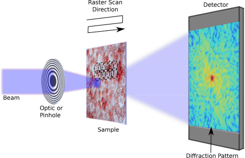
Figure 1. Simplified ptychographic setup showing a Cartesian grid used for the overlapping raster scan positions [25].

Now consider the simplest, 2-part ptychographic set-up: the object domain is the union of two overlapping square grids, one of which is the translate of the other square grid. Denote the two square grids by ${\mathcal{M}}^{0}$ and ${\mathcal{M}}^{\mathbf{t}}$ which is the shift of ${\mathcal{M}}^{0}$ by the displacement vector $\mathbf{t}=(t_{1},t_{2})\in\mathbb{Z}^{2}$. We shall make the overlap assumption

(3) $$\left|{\mathcal{M}}^{0}\cap{\mathcal{M}}^{\mathbf{t}}\cap{\hbox{\rm supp}}{(f)}\right|\geq 2,$$

where $\left|\cdot\right|$ denotes the cardinality of a set, i.e. the intersection of the two grids contains at least two points from the support of the object.

Let $f^{\mathbf{t}}$ be the unknown object restricted to ${\mathcal{M}}^{\mathbf{t}}$ and $\Phi^{\mathbf{t}}$ the ODFT on ${\mathcal{M}}^{\mathbf{t}}$. We write the object function as $f=f^{0}\cup f^{\mathbf{t}}$ where $f^{0}(\mathbf{m})=f^{\mathbf{t}}(\mathbf{m})$ for all $\mathbf{m}\in{\mathcal{M}}^{0}\cap{\mathcal{M}}^{\mathbf{t}}$. Let $f^{0}$ and $f^{\mathbf{t}}$ be respectively illuminated with the mask $\mu^{0}$ and the mask $\mu^{\mathbf{t}}$ on where $\mu^{\mathbf{t}}({\mathbf{n}})=\mu^{0}({\mathbf{n}}-\mathbf{t}),$ for all ${\mathbf{n}}\in{\mathcal{M}}^{\mathbf{t}}$.

For multi-part ptychography, let the object domain be contained in the union of the shifted square grids:

(4) $${\hbox{\rm supp}}(f)\subseteq\bigcup_{\mathbf{t}\in{\mathcal{T}}}{\mathcal{M}}^{\mathbf{t}}$$

where ${\mathcal{T}}$ is a set of shifts. We can write

(5) $$f=\bigcup_{\mathbf{t}\in{\mathcal{T}}}f^{\mathbf{t}}.$$

Analogous to (3) we assume that for every ${\mathcal{M}}^{\mathbf{t}_{1}}\cap{\hbox{\rm supp}}(f)\neq\emptyset,\mathbf{t}_{1}\in{\mathcal{T}}$, there is another ${\mathcal{M}}^{\mathbf{t}_{2}},\mathbf{t}_{2}\in{\mathcal{T}},\mathbf{t}_{2}\neq\mathbf{t}_{1}$ such that

(6) $$\left|{\mathcal{M}}^{\mathbf{t}_{1}}\cap{\mathcal{M}}^{\mathbf{t}_{2}}\cap{\hbox{\rm supp}}(f)\right|\geq 2.$$

In other words, every connected component of the object is contained in the union of at least two distinct masks, whose intersection contains at least two points of the object support. Since the support of the object is often not known precisely, some illuminations may totally miss the object and produce no useful information. These illuminations and the resulting data are easily recognized and should be discarded.

1.2. A minimalist ptychographic scheme

Although our uniqueness theorem and local convergence analysis are for general ptychographic measurement schemes satisfying (6), we will consider the following more structured scheme for numerical experiments and explicit estimation of convergence rate. We call this practical scheme the minimalist scheme because each object pixel participates exactly in four diffraction patterns (two in each direction) and two adjacent mask domains have the minimum (i.e. $50\%$) overlap.

Suppose the initial mask domain ${\mathcal{M}}^{0}$ is $m\times m$ ($m$ is an even integer) and an adjacent domain is obtained by shifting $m/2$ in either direction. To cover each object pixel exactly four times (two in each direction) we assume $m=2n/q$ with an integer $q$. This amounts to $q^{2}$ diffraction patterns. In other words, we consider the shift $T^{kl}$ corresponding to the displacement $\mathbf{t}_{kl}={m\over 2}(k,l)$, with $k\in\{0,1,\cdots,q-1\},\leavevmode\nobreak\ l\in\{0,1,\cdots,q-1\}$. When $k=q-1$ or $l=q-1$ we assume for simplicity that the shifted mask is wrapped around into the other end of the object domain (i.e. the periodic boundary condition). Four times coverage and four times oversampling in each diffraction pattern together produce the total number $q^{2}(2m-1)^{2}\approx 16n^{2}$ of data.

We emphasize two features of the minimalist scheme: (i) The scheme has a fixed total oversampling ratio ($\approx 16$) independent of the total number of shifted masks, $q^{2}$; (ii) This scheme has the minimum ($50\%$) overlap between two adjacent masks while maintaining the same number of coverage (i.e. 4) for every pixel of the object. Note that the $50\%$ overlap is lower than the required overlap found empirically (i.e. $60\%-70\%$) from previous studies [2, 21].

These features are highly desirable in practice because an efficient ptychographic scheme should not only collect as few data as possible overall but also deploy as few shifted masks as possible.

With this minimalist ptychographic scheme, we study analytically and numerically how $q$ and the nature of the mask affect ptychographic reconstruction.

1.3. Main contributions

The first result of the present work is the almost sure uniqueness of ptychographic solution with an independent random mask under the minimum overlap condition (6) (Theorem 2.3 and Corollary 2.4).

In this connection, Iwen et al. [18] proved a uniqueness theorem for the ptychographic scheme where all possible shifts of a damped and windowed Fourier transform are used, i.e. the overlap percentage between two adjacent mask domains is at the maximum. In our notation, this amounts to $n^{2}$ oversampled diffraction patterns totaling $(2m-1)^{2}n^{2}$ number of data. Their uniqueness theorem also holds with probability $1-{\mathcal{O}}(\ln^{-2}{n}\ln^{-3}(\ln n))$ after randomly selecting a subset of ${\mathcal{O}}(n^{2}\ln^{2}{n}\ln^{3}(\ln n))$ data (assuming $m$ is at least poly-log in $n$).

In Section 3, we establish local, geometric convergence (Theorem 3.4) for the alternating projections (AP) and the Douglas-Rachford (DR) algorithms under the minimum overlap condition (6). We also prove the uniqueness of the DR fixed point in the object domain (Proposition 3.1) and give an easily verifiable criterion for distinguishing the true solution among many AP fixed points (Proposition 3.3).

In comparison, Wen et al. [29] proposed alternating direction methods (ADM), including DR, for ptychographic reconstruction and demonstrated good numerical performance. Hesse et al. [14] proved global convergence to a critical point for a proximal-regularized alternating minimization formulation of blind ptychography. Many critical points, however, may co-exist and there is no easy way of distinguishing the true solution from the rest. Neither of these papers establishes uniqueness, convergence to the true solution or the geometric sense of convergence.

We also give a bound on the convergence rate of AP and DR for the minimalist scheme introduced in Section 1.2 (Proposition 4.1). The bound shows that the convergence rate can deteriorate rapidly as $q$ becomes large, indicating that the best performing $q$ are in the small and medium ranges. Our numerical experiments in Section 5 bear this prediction out nicely, focusing on two kinds of masks: (independent or correlated) random masks and the Fresnel mask.

Finally we prove that for $q=2$, twin image exists in ptychography with the Fresnel mask at certain values of the Fresnel number and causes the reconstruction error to spike (Propositions A.1 and A.2). As the Fresnel mask is most convenient to fabricate, this result gives a guideline for avoiding poor-performing masks.

We summarize our numerical findings in the Conclusion (Section 6).

2. Uniqueness of ptychographic solution

First we recall some basic results from nonptychographic phase retrieval where the mask $\mu$ and the unknown object $f$ have the same dimension.

The $z$-transform

$$F(\mathbf{z})=\sum_{{\mathbf{n}}}f({\mathbf{n}})\mathbf{z}^{-{\mathbf{n}}}$$

of $f$ is a polynomial in $\mathbf{z}^{-1}$ and can be factorized uniquely into the product of irreducible polynomials $F_{k}(\mathbf{z})$ and a monomial in $\mathbf{z}^{-1}$

(7) $$F(\mathbf{z})=\alpha\mathbf{z}^{-{\mathbf{n}}_{0}}\prod_{k=1}^{p}F_{k}(\mathbf{z}),$$

where ${\mathbf{n}}_{0}$ is a vector of nonnegative integers and $\alpha$ is a complex coefficient.

Proposition 2.1.

[13] Let the $z$-transform $F(\mathbf{z})$ of a finite complex-valued array $\{f({\mathbf{n}})\}$ be given by

(8) $$F(\mathbf{z})=\alpha\mathbf{z}^{-\mathbf{m}}\prod_{k=1}^{p}F_{k}(\mathbf{z}),\quad\mathbf{m}\in\mathbb{N}^{d},\alpha\in\mathbb{C}$$

where $F_{k},k=1,...,p$ are nontrivial irreducible polynomials. Let $G(\mathbf{z})$ be the $\mathbf{z}$-transform of another finite array $g({\mathbf{n}})$. Suppose $|F(\mathbf{w})|=|G(\mathbf{w})|,\forall\mathbf{w}\in[0,1]^{d}$. Then $G(\mathbf{z})$ must have the form

$$G(\mathbf{z})=|\alpha|e^{{\rm i}\theta}\mathbf{z}^{-{\mathbf{p}}}\left(\prod_{k\in I}F_{k}(\mathbf{z})\right)\left(\prod_{k\in I^{c}}F_{k}^{*}(1/\mathbf{z}^{*})\right),\quad{\mathbf{p}}\in\mathbb{N}^{d},\theta\in\mathbb{R}$$

where $I$ is a subset of $\{1,2,...,p\}$.

Line object: $f$ is a line object if the convex hull of the object support in $\mathbb{R}^{d}$ is a line segment.

Proposition 2.2.

[7] Suppose $f$ is not a line object and let the mask $\mu$’s phase be continuously and independently distributed. Then with probability one the only irreducible factor of the $z$-transform of the masked object $\tilde{f}({\mathbf{n}})=f({\mathbf{n}})\mu({\mathbf{n}})$ is a monomial of $\mathbf{z}^{-1}$.

The following uniqueness theorem is our first theoretical result.

Theorem 2.3.

Suppose that the assumptions of Proposition 2.2 hold and that

$$\left|{\mathcal{M}}^{0}\cap{\mathcal{M}}^{\mathbf{t}}\cap{\hbox{\rm supp}}{(f)}\right|\geq 2.$$

Then with probability one $f$ is uniquely determined, up to a global phase factor, by the measurement data $b=|A^{*}f|$.

Proof.

Let $g({\mathbf{n}})$ be another array that vanishes outside ${\mathcal{M}}^{0}\cup{\mathcal{M}}^{\mathbf{t}}$ and produces the same masked Fourier magnitude data. By Proposition 2.1 and 2.2, $g$ has the following possibilities: In ${\mathcal{M}}^{0}$, $g$ has two alternatives

(9) $$g({\mathbf{n}}) = \left\{\begin{matrix}e^{{\rm i}\theta_{1}}f^{0}({\mathbf{n}}+\mathbf{m}_{1})\mu^{0}({\mathbf{n}}+\mathbf{m}_{1})/\mu^{0}({\mathbf{n}})\\ e^{{\rm i}\theta_{1}}\bar{f}^{0}(\mathbf{N}-{\mathbf{n}}+\mathbf{m}_{1})\bar{\mu}^{0}(\mathbf{N}-{\mathbf{n}}+\mathbf{m}_{1})/\mu^{0}({\mathbf{n}}),\end{matrix}\right.\quad\forall{\mathbf{n}}\in{\mathcal{M}}^{0}$$

and

(10) $$g({\mathbf{n}}) = \left\{\begin{matrix}e^{{\rm i}\theta_{2}}f^{\mathbf{t}}({\mathbf{n}}+\mathbf{m}_{2})\mu^{\mathbf{t}}({\mathbf{n}}+\mathbf{m}_{2})/\mu^{\mathbf{t}}({\mathbf{n}})\\ e^{{\rm i}\theta_{2}}\bar{f}^{\mathbf{t}}(\mathbf{N}-{\mathbf{n}}+\mathbf{m}_{2})\bar{\mu}^{\mathbf{t}}(\mathbf{N}-{\mathbf{n}}+\mathbf{m}_{2})/\mu^{\mathbf{t}}({\mathbf{n}}),\end{matrix}\right.\quad\forall{\mathbf{n}}\in{\mathcal{M}}^{\mathbf{t}}$$

for some $\mathbf{m}_{1},\mathbf{m}_{2}\in\mathbb{Z}^{d},\theta_{1},\theta_{2}\in\mathbb{R}$.

We now focus on the intersection ${\mathcal{M}}^{0}\cap{\mathcal{M}}^{\mathbf{t}}$ where (9) and (10) are both defined. We have then four scenarios from the crossover of the alternatives in (9) and (10).

First of all, if, for all ${\mathbf{n}}\in{\mathcal{M}}^{0}\cap{\mathcal{M}}^{\mathbf{t}}$,

$$g({\mathbf{n}}) = e^{{\rm i}\theta_{1}}f^{0}({\mathbf{n}}+\mathbf{m}_{1})\mu^{0}({\mathbf{n}}+\mathbf{m}_{1})/\mu^{0}({\mathbf{n}})$$

$$= e^{{\rm i}\theta_{2}}f^{\mathbf{t}}({\mathbf{n}}+\mathbf{m}_{2})\mu^{\mathbf{t}}({\mathbf{n}}+\mathbf{m}_{2})/\mu^{\mathbf{t}}({\mathbf{n}})$$

then

(12) $$e^{{\rm i}\theta_{1}}f^{0}({\mathbf{n}}+\mathbf{m}_{1})\mu^{0}({\mathbf{n}}+\mathbf{m}_{1})/\mu^{0}({\mathbf{n}})=e^{{\rm i}\theta_{2}}f^{\mathbf{t}}({\mathbf{n}}+\mathbf{m}_{2})\mu^{0}({\mathbf{n}}-\mathbf{t}+\mathbf{m}_{2})/\mu^{0}({\mathbf{n}}-\mathbf{t}).$$

Clearly, $f({\mathbf{n}}+\mathbf{m}_{1})$ and $f^{\mathbf{t}}({\mathbf{n}}+\mathbf{m}_{2})$ must simultaneously be zero or nonzero. When they are nonzero, we obtain by taking logarithm on both sides

$${\rm i}\theta_{1}+\ln{f^{0}({\mathbf{n}}+\mathbf{m}_{1})}+\ln{\mu^{0}({\mathbf{n}}+\mathbf{m}_{1})}+\ln{\mu^{0}({\mathbf{n}}-\mathbf{t})}$$

$$= {\rm i}\theta_{2}+\ln{f^{\mathbf{t}}({\mathbf{n}}+\mathbf{m}_{2})}+\ln{\mu^{0}({\mathbf{n}}-\mathbf{t}+\mathbf{m}_{2})}+\ln{\mu^{0}({\mathbf{n}})}$$

which holds up to a multiple of $2\pi$. The four random variables

$$\ln{\mu^{0}({\mathbf{n}}+\mathbf{m}_{1})},\leavevmode\nobreak\ \ln{\mu^{0}({\mathbf{n}}-\mathbf{t})},\leavevmode\nobreak\ \ln{\mu^{0}({\mathbf{n}}-\mathbf{t}+\mathbf{m}_{2})},\leavevmode\nobreak\ \ln{\mu^{0}({\mathbf{n}})}$$

can not cancel one another unless either $\mathbf{m}_{1}=\mathbf{m}_{2}=0$ or $(\mathbf{t}=0\leavevmode\nobreak\ \&\leavevmode\nobreak\ \mathbf{m}_{1}=\mathbf{m}_{2})$. When the continuous random variables do not cancel one another, (2) fails to hold true almost surely.

On the other hand, for $\mathbf{m}_{1}=\mathbf{m}_{2}=0$ (since $\mathbf{t}\neq 0$), it follows from (2) that

$$g({\mathbf{n}})=e^{{\rm i}\theta_{1}}f^{0}({\mathbf{n}})=e^{{\rm i}\theta_{2}}f^{\mathbf{t}}({\mathbf{n}}),\quad{\mathbf{n}}\in{\mathcal{M}}^{0}\cap{\mathcal{M}}^{\mathbf{t}}.$$

Since $f^{0}({\mathbf{n}})=f^{\mathbf{t}}({\mathbf{n}})$, we have $\theta_{1}=\theta_{2}$. It follows then from (9)-(10) that $g=e^{{\rm i}\theta_{1}}(f^{0}\cup f^{\mathbf{t}})$.

The other three scenarios can be similarly dealt with. Consider the next scenario where for ${\mathbf{n}}\in{\mathcal{M}}^{0}\cap{\mathcal{M}}^{\mathbf{t}}$

$$g({\mathbf{n}}) = e^{{\rm i}\theta_{1}}f^{0}({\mathbf{n}}+\mathbf{m}_{1})\mu^{0}({\mathbf{n}}+\mathbf{m}_{1})/\mu^{0}({\mathbf{n}})$$

$$= e^{{\rm i}\theta_{2}}\bar{f}^{\mathbf{t}}(\mathbf{N}-{\mathbf{n}}+\mathbf{m}_{2})\bar{\mu}^{\mathbf{t}}(\mathbf{N}-{\mathbf{n}}+\mathbf{m}_{2})/\mu^{\mathbf{t}}({\mathbf{n}}).$$

Taking logarithm and rearranging terms we have

$${\rm i}\theta_{1}+\ln{f^{0}({\mathbf{n}}+\mathbf{m}_{1})}+\ln{\mu^{0}({\mathbf{n}}+\mathbf{m}_{1})}+\ln{\mu^{0}({\mathbf{n}}-\mathbf{t})}+\ln{\mu^{0}(\mathbf{N}-{\mathbf{n}}-\mathbf{t}+\mathbf{m}_{2})}$$

$$= {\rm i}\theta_{2}+\ln{\bar{f}^{\mathbf{t}}(\mathbf{N}-{\mathbf{n}}+\mathbf{m}_{2})}+\ln{\mu^{0}({\mathbf{n}})}$$

The four random variables

$$\ln{\mu^{0}({\mathbf{n}}+\mathbf{m}_{1})},\leavevmode\nobreak\ \ln{\mu^{0}({\mathbf{n}}-\mathbf{t})},\leavevmode\nobreak\ \ln{\mu^{0}(\mathbf{N}-{\mathbf{n}}-\mathbf{t}+\mathbf{m}_{2})},\leavevmode\nobreak\ \ln{\mu^{0}({\mathbf{n}})}$$

can not cancel one another since $\mathbf{t}\neq 0$. As a result, (2) holds true with probability zero.

The argument for ruling out the third scenario

$$g({\mathbf{n}}) = e^{{\rm i}\theta_{1}}\bar{f}^{0}(\mathbf{N}-{\mathbf{n}}+\mathbf{m}_{1})\bar{\mu}^{0}(\mathbf{N}-{\mathbf{n}}+\mathbf{m}_{1})/\mu^{0}({\mathbf{n}})$$

$$= e^{{\rm i}\theta_{2}}f^{\mathbf{t}}({\mathbf{n}}+\mathbf{m}_{2})\mu^{\mathbf{t}}({\mathbf{n}}+\mathbf{m}_{2})/\mu^{\mathbf{t}}({\mathbf{n}})$$

is the same as for the second scenario.

Now consider the fourth scenario

$$g({\mathbf{n}}) = e^{{\rm i}\theta_{1}}\bar{f}^{0}(\mathbf{N}-{\mathbf{n}}+\mathbf{m}_{1})\bar{\mu}^{0}(\mathbf{N}-{\mathbf{n}}+\mathbf{m}_{1})/\mu^{0}({\mathbf{n}})$$

$$= e^{{\rm i}\theta_{2}}\bar{f}^{\mathbf{t}}(\mathbf{N}-{\mathbf{n}}+\mathbf{m}_{2})\bar{\mu}^{\mathbf{t}}(\mathbf{N}-{\mathbf{n}}+\mathbf{m}_{2})/\mu^{\mathbf{t}}({\mathbf{n}})$$

which after taking logarithm and rearranging terms becomes

$${\rm i}\theta_{1}+\ln{\bar{f}^{0}(\mathbf{N}-{\mathbf{n}}+\mathbf{m}_{1})}+\ln{\mu^{0}(\mathbf{N}-{\mathbf{n}}-\mathbf{t}+\mathbf{m}_{2})}+\ln{\mu^{0}({\mathbf{n}}-\mathbf{t})}$$

$$= {\rm i}\theta_{2}+\ln{\bar{f}^{\mathbf{t}}(\mathbf{N}-{\mathbf{n}}+\mathbf{m}_{2})}+\ln{\mu^{0}(\mathbf{N}-{\mathbf{n}}+\mathbf{m}_{1})}+\ln{\mu^{0}({\mathbf{n}})}.$$

Since $\mathbf{t}\neq 0$, the four random variables

$$\ln{\mu^{0}(\mathbf{N}-{\mathbf{n}}-\mathbf{t}+\mathbf{m}_{2})},\leavevmode\nobreak\ \ln{\mu^{0}({\mathbf{n}}-\mathbf{t})},\leavevmode\nobreak\ \ln{\mu^{0}(\mathbf{N}-{\mathbf{n}}+\mathbf{m}_{1})},\leavevmode\nobreak\ \ln{\mu^{0}({\mathbf{n}})}$$

cancel one another only when

$$\mathbf{N}-{\mathbf{n}}-\mathbf{t}+\mathbf{m}_{2} = {\mathbf{n}}$$

$${\mathbf{n}}-\mathbf{t} = \mathbf{N}-{\mathbf{n}}+\mathbf{m}_{1}$$

or equivalently

$$\mathbf{m}_{2} = 2{\mathbf{n}}-\mathbf{N}+\mathbf{t}$$

$$\mathbf{m}_{1} = 2{\mathbf{n}}-\mathbf{N}-\mathbf{t}$$

which can not hold true simultaneously for more than one ${\mathbf{n}}$ for any given $\mathbf{m}_{1},\mathbf{m}_{2}$. This is ruled out by the assumption that ${\mathcal{M}}^{0}\cap{\mathcal{M}}^{\mathbf{t}}\cap{\hbox{\rm supp}}(f)$ contains at least two points.

In summary, the only possibility is that

$$g=e^{{\rm i}\theta}(f^{0}\cup f^{\mathbf{t}})=e^{{\rm i}\theta}f$$

for some $\theta\in\mathbb{R}$, which is what we set out to prove.

∎

The divide-overlap-and-conquer strategy is readily extendable to the multi-part setting.

Corollary 2.4.

Consider the multi-part ptychography (4)-(5). Suppose that the assumptions of Proposition 2.2 hold and that for every ${\mathcal{M}}^{\mathbf{t}_{1}}\cap{\hbox{\rm supp}}(f)\neq\emptyset,\mathbf{t}_{1}\in{\mathcal{T}}$ there is another $\mathbf{t}_{2}\in{\mathcal{T}},\mathbf{t}_{2}\neq\mathbf{t}_{1},$ such that

(16) $$\left|{\mathcal{M}}^{\mathbf{t}_{1}}\cap{\mathcal{M}}^{\mathbf{t}_{2}}\cap{\hbox{\rm supp}}(f)\right|\geq 2.$$

Then with probability one $f$ is determined uniquely, up to a constant phase factor for each connected component of $f$, by the ptychographic data

(17) $$\left\{\left|\Phi^{\mathbf{t}}(\mu^{\mathbf{t}}\odot f^{\mathbf{t}})\right|:\mathbf{t}\in{\mathcal{T}}\right\}.$$

The constant phase factor becomes global, i.e. the same one for the whole object, if

(18) $$\bigcup\left\{{\mathcal{M}}^{\mathbf{t}}:{\mathcal{M}}^{\mathbf{t}}\cap f\neq\emptyset,\mathbf{t}\in{\mathcal{T}}\right\}\quad\mbox{is a connected set}.$$

Remark 2.5.

Clearly the result still holds when some of the shifted masks do not intersect with the object. This has a practical relevance as the support of the object is often not precisely known and some illuminations can totally miss the object. Of course, these illuminations produce no useful information and should be discarded.

When the condition (18) fails, the whole ptychographic problem breaks down into a set of separate independent subproblems, each with the data corresponding to a connected component of $\bigcup\left\{{\mathcal{M}}^{\mathbf{t}}:{\mathcal{M}}^{\mathbf{t}}\cap f\neq\emptyset,\mathbf{t}\in{\mathcal{T}}\right\}$.

Proof.

Let $\mathbf{t}_{1},\mathbf{t}_{2}\in{\mathcal{T}}$ be any pair of shifts satisfying the overlapping property (16). Then by Theorem 2.3, $f^{\mathbf{t}_{1}}\cup f^{\mathbf{t}_{2}}$ is uniquely determined, up to a constant phase factor, by the data

$$\left\{\left|\Phi^{\mathbf{t}_{j}}(\mu^{\mathbf{t}_{j}}\odot f^{\mathbf{t}_{j}})\right|:j=1,2\right\}$$

with probability one where $\odot$ denotes the Hadamard (i.e. componentwise) product. Since $f$ is the union of all such pairs $f^{\mathbf{t}_{1}}\cup f^{\mathbf{t}_{2}}$, $f$ is uniquely determined, up to a constant phase factor for each connected component of $f$, by the data (17), with probability one.

The constant phase factor ambiguity for every connected component may not be the same since some masks may have no intersection with the object. Once condition (18) is valid, the constant phase factor must be the same for the whole object. ∎

3. Fixed point algorithms

To describe the reconstruction algorithms, it is most convenient to resort to the vector-matrix notation where we use $\mathbb{C}^{N}$ ($N=$ the total number of pixels in the object = $n^{2}$) as the object space and $\mathbb{C}^{M}$ ($M=$ the total number of measurement data $=m^{2}$) as the the data space before taking the modulus of the diffracted field. We use $\|\cdot\|$ to denote the vector norm as well as the Frobenius norm when the object is written as a matrix.

A phase-masked measurement gives rise to an isometric matrix in the non-ptychographic setting

(19) $$\hbox{\rm(1-pattern nonptychographic matrix)}\quad A^{*}=c\Phi\,\,\hbox{\rm diag}\{\mu\},$$

where the constant $c$ is chosen to normalize $A^{*}$ such that $AA^{*}=I$. The 2-pattern ptychography matrix $A^{*}$ can be written as

(20) $$\hbox{(2-pattern ptychography matrix)}\quad A^{*}=c\left[\begin{matrix}\Phi^{0}\leavevmode\nobreak\ \hbox{\rm diag}\{\mu^{0}\}&0\\ 0&\Phi^{\mathbf{t}}\leavevmode\nobreak\ \hbox{\rm diag}\{\mu^{\mathbf{t}}\}\end{matrix}\right]$$

where the first and second mask domains overlap due to the nature of a ptychographic scheme.

The propagation matrix $A^{*}$ for multi-part ptychography is constructed analogous to (20) by stacking $\Phi^{\mathbf{t}}\leavevmode\nobreak\ \hbox{\rm diag}\{\mu^{\mathbf{t}}\},\leavevmode\nobreak\ \forall\mathbf{t}\in{\mathcal{T}}$ in the proper order. For algorithmic analysis, we normalize the columns of $A^{*}$ so that $A^{*}$ is isometric.

Let $b\equiv|A^{*}f|\in\mathbb{R}^{M}$. For any $y\in\mathbb{C}^{M}$, $\mbox{\rm sgn}(y)\in\mathbb{C}^{M}$ is defined as

$$\mbox{\rm sgn}(y)[j]=\left\{\begin{matrix}1&\mbox{if $y[j]=0$}\\ y[j]/|y[j]|&\mbox{else. }\end{matrix}\right.$$

Ptychography can be formulated as the following feasibility problem in the Fourier domain

(21) $$\hbox{Find}\quad\hat{y}\in A^{*}{\mathcal{X}}\cap\mathcal{Y},\quad\mathcal{Y}:=\{y\in\mathbb{C}^{M}:|y|=b\}.$$

Let $P_{1}$ be the projection onto $A^{*}{\mathcal{X}}$ and $P_{2}$ the projection onto $\mathcal{Y}$:

(22) $$P_{1}y=A^{*}Ay,\quad P_{2}y=b\odot{\mbox{\rm sgn}(y)}.$$

The following are two of the most widely used iterative algorithms for solving feasibility problems.

• (23) $$y^{(k+1)}=P_{1}P_{2}y^{(k)}$$

• (24) $$y^{(k+1)} = y^{(k)}+P_{1}(2P_{2}-I)y^{(k)}-P_{2}y^{(k)}$$

As the final output of either algorithm, the object estimate is given by $x^{(k)}=Ay^{(k)}$.

As we discuss below, AP and DR have their respective strengths and weaknesses and we will combine their strengths in ptychographic reconstruction.

3.1. Fixed point

To accommodate the arbitrariness of the phase of zero components, we call $y_{*}$ a Fourier-domain DR fixed point if there exists

$$u\in U=\{u=(u[i])\in\mathbb{C}^{M}:|u[i]|=1,\,\,\forall i\}\$$

satisfying

(25) $$u\in U,\quad u[j]=1,\quad\hbox{whenever}\leavevmode\nobreak\ y_{*}[j]\neq 0$$

such that the DR fixed point equation holds

(26) $$A^{*}A\left(2b\odot\mbox{\rm sgn}({y_{*}})\odot u-y_{*}\right)=b\odot\mbox{\rm sgn}({y_{*}})\odot u.$$

Note that if the sequence of iterates $y^{(k)}$ converges a limit $y_{\infty}$ that has no zero component, then the limit $y_{\infty}$ is a Fourier domain DR fixed point with $u\equiv 1$.

Let $x_{*}=Ay_{*}$ be the corresponding object-domain fixed point. Define another object estimate

(27) $$\hat{x} = A\left(2b\odot\mbox{\rm sgn}(y_{*})\odot u-y_{*}\right)$$

for some $u$ satisfying (25).

We have from (26)

(28) $$A^{*}\hat{x}=b\odot\mbox{\rm sgn}(y_{*})\odot u$$

which implies

(29) $$|A^{*}\hat{x}| = |A^{*}f|$$

(30) $$\arg(A^{*}\hat{x}) = \arg(\mbox{\rm sgn}(y_{*})\odot u)\quad\hbox{on}\leavevmode\nobreak\ {\hbox{\rm supp}}(b).$$

Proposition 3.1.

Under the assumptions of Corollary 2.4 including (18), $\hat{x}=x_{*}=e^{{\rm i}\theta}f$ for some constant $\theta\in\mathbb{R}$ almost surely.

Proof.

By Theorem 2.3 and Corollary 2.4, (29) implies that $\hat{x}=e^{{\rm i}\theta}f$ for some constant $\theta\in\mathbb{R}$. To complete the proof, we only need to show $e^{{\rm i}\theta}f=x_{*}$.

By (30) and the identity $\hat{x}=e^{{\rm i}\theta}f$, we have

(31) $$e^{{\rm i}\theta}\mbox{\rm sgn}(A^{*}f)=\mbox{\rm sgn}(y_{*})\odot u\quad\hbox{on}\leavevmode\nobreak\ {\hbox{\rm supp}}(b).$$

Substituting (31) into (27) we obtain

$$e^{{\rm i}\theta}f=A\left(2b\odot e^{{\rm i}\theta}\mbox{\rm sgn}(A^{*}f)-y_{*}\right)=2e^{{\rm i}\theta}A\left(b\odot\mbox{\rm sgn}(A^{*}f)\right)-Ay_{*}=2e^{{\rm i}\theta}f-x_{*}$$

where the last identity follows from the isometry of $A^{*}$ and the definition of $x_{*}$. Hence $e^{{\rm i}\theta}f=x_{*}$ as claimed. ∎

Likewise, we call $x_{*}$ an AP fixed point if for some $u\in U$

(32) $$x_{*}=A\left(b\odot u\odot\mbox{\rm sgn}({A^{*}x_{*}})\right).$$

The following result identifies any AP limit point with an AP fixed point.

Proposition 3.2.

Under the assumptions of Corollary 2.4, every limit point of AP iterates $\{x^{(k)}\}$ is an AP fixed point in the sense (32).

The proof of Proposition 3.2 can be adapted from [5] verbatim and is omitted.

How do we distinguish the true ptychographic solution from the possibly many AP fixed points (in view of recurring numerical stagnation from random initialization)?

Consider the inequality

(33) $$\|x_{*}\|=\left\|A\left(\mbox{\rm sgn}\{{A^{*}x_{*}}\}\odot b\odot u\right)\right\|\leq\left\|\mbox{\rm sgn}\{A^{*}x_{*}\}\odot b\odot u\right\|=\|b\|.$$

Clearly $\|x_{*}\|=\|b\|$ holds if and only if the inequality in Eq. (33) is an equality, which is true only when

(34) $$\mbox{\rm sgn}\{A^{*}x_{*}\}\odot b\odot u=A^{*}z\quad\textrm{ for some $z\in\mathbb{C}^{n}$}.$$

Since $AA^{*}=I$ the fixed point equation (32) implies $z=x_{*}$ and hence

$$\mbox{\rm sgn}\{A^{*}x_{*}\}\odot b\odot u=A^{*}x_{*}.$$

Thus $b=|A^{*}x_{*}|$ implying $x_{*}$ is the ptychographic solution by Corollary 2.4. Therefore

Proposition 3.3.

Under the assumptions of Corollary 2.4 including (18), all AP fixed points $x_{*}$ satisfy $\|x_{*}\|\leq\|b\|$ and $x_{*}=f$ is the only AP fixed point satisfying $\|x_{*}\|=\|b\|$.

While we do not have the assurance of a unique AP fixed point in comparison with DR, AP has a better convergence rate than DR as we discuss next.

3.2. Local convergence

Theorem 3.4.

Under the assumptions of Corollary 2.4 including (18), let $A^{*}$ be the measurement matrix and

(35) $$B:=A\,\,\hbox{\rm diag}\left\{\mbox{\rm sgn}({A^{*}f})\right\}\in\mathbb{C}^{N\times M}.$$

Then

(36) $$\gamma=\max\{\|\Im(B^{*}u)\|:u\in\mathbb{C}^{N},\leavevmode\nobreak\ u\perp{\rm i}f,\leavevmode\nobreak\ \|u\|=1\}<1.$$

Moreover, for any given $0<\epsilon<1-\gamma$, if the initial point $y^{(1)}$ is chosen such that

$$\|\alpha^{(1)}x^{(1)}-f\|:=\min_{\alpha\in\mathbb{C}\atop|\alpha|=1}\|\alpha x^{(1)}-f\|\quad\mbox{ is sufficiently small,}$$

then we have the geometric convergence

(37) DR: $$\min_{\alpha\in\mathbb{C}\atop|\alpha|=1}\|\alpha x^{(k)}-f\|\leq(\gamma+\epsilon)^{k-1}\|\alpha^{(1)}x^{(1)}-f\|,$$

(38) AP: $$\min_{\alpha\in\mathbb{C}\atop|\alpha|=1}{\|\alpha x^{(k)}-f\|}\leq(\gamma^{2}+\epsilon)^{k-1}{\|\alpha^{(1)}x^{(1)}-f\|}.$$

For $\gamma<1$, the convergence rate $\gamma^{2}$ of AP is better than the convergence rate $\gamma$ of DR. The proof is omitted as can be adapted to the ptychographic setting from the nonptychographic setting of [5, 4] without major changes. However, we will elaborate on the meaning of and give an estimate for (36) below.

First let us explain the connection between the matrix $B$ in (35) and the subdifferential of the iterative map. To this end, we consider the isomorphism $\mathbb{C}^{N}\cong\mathbb{R}^{2N}$ via the map

$$G(x):=\left[\begin{matrix}\Re(x)\\ \Im(x)\end{matrix}\right],\quad G(-ix)=\left[\begin{matrix}\Im(x)\\ -\Re(x)\end{matrix}\right]$$

and define the real-valued matrix

(41) $$\mathcal{B} = \left[\begin{array}[]{c}\Re(B)\\ \Im(B)\end{array}\right]\in\mathbb{R}^{2N\times M}.$$

Denote the AP map by

$$F_{\rm AP}=P_{1}P_{2}$$

and the DR map by

$$F_{\rm DR}=I+P_{1}(2P_{2}-I)-P_{2}.$$

From straightforward but somewhat tedious algebra, we have

(42) $$G(dF_{\rm AP}(f)\xi)=G({\rm i}B\Im(B^{*}\xi)),\quad\forall\xi\in\mathbb{C}^{N}$$

or equivalently

(43) $$G(-{\rm i}dF_{\rm AP}(f)\xi)={\mathcal{B}}{\mathcal{B}}^{\top}G(-{\rm i}\xi),\quad\forall\xi\in\mathbb{C}^{N}$$

and

(44) $$dF_{\rm DR}(f)\eta=\hbox{\rm diag}[\mbox{\rm sgn}(A^{*}f)]J\hbox{\rm diag}[\overline{\mbox{\rm sgn}(A^{*}f)}]\eta$$

where

(45) $$Jy=(I-B^{*}B)\Re(y)+{\rm i}B^{*}B\Im(y).$$

Eq. (42)-(45) exhibit the central role of $B$ in the subdifferentials $dF_{\rm AP},dF_{\rm DR}$ at the point $f$. For detailed derivation we refer the reader to [5, 4].

Next we explain the meaning of the variational principle (36). Let $\lambda_{1}\geq\lambda_{2}\geq\ldots\geq\lambda_{2N}\geq 0$ be the singular values of

$$\mathcal{B}^{\top}=\left[\Re(B)^{\top}\quad\Im(B)^{\top}\right]\in\mathbb{R}^{M\times 2N}.$$

Since the complex matrix $B^{*}$ is isometric, we have $\lambda_{k}^{2}+\lambda_{2N+1-k}^{2}=1,\forall k=1,\ldots,2N$.

By definition, for any $x\in\mathbb{C}^{N}$

$$B^{*}x=\hbox{\rm diag}\left[\overline{\mbox{\rm sgn}({A^{*}f})}\right]A^{*}x$$

and hence

(46) $${\mathcal{B}}^{\top}G(f)=\Re[B^{*}f]=|A^{*}f|.$$

On the other hand, we have by isometry of $A^{*}$

(47) $${\mathcal{B}}|A^{*}f|=\left[\begin{matrix}\Re(B|A^{*}f|)\\ \Im(B|A^{*}f|)\end{matrix}\right]=\left[\begin{matrix}\Re(AA^{*}f)\\ \Im(AA^{*}f)\end{matrix}\right]=\left[\begin{matrix}\Re(f)\\ \Im(f)\end{matrix}\right]=G(f).$$

Eq. (46) and (47) imply $\lambda_{1}=1$ and $G(f)$ is a leading singular vector of ${\mathcal{B}}^{\top}$. We can also easily verify

(48) $${\mathcal{B}}^{\top}G(-{\rm i}f)=\Im[B^{*}f]=0$$

and hence $G(-{\rm i}f)$ is a corresponding singular vector to $\lambda_{2N}=0$.

Note again $\Im[B^{*}u]={\mathcal{B}}^{\top}G(-{\rm i}u).$ The orthogonality condition ${\rm i}u\perp f$ is equivalent to $G(f)\perp G(-{\rm i}u).$ Therefore $\gamma$ defined in (36) is the second largest singular value $\lambda_{2}$ of ${\mathcal{B}}^{\top}$ and admits the variational principle

(49) $$\gamma = \max\{\|{\mathcal{B}}^{\top}u\|:{u\in\mathbb{R}^{2N},u\perp G(f)},\|u\|=1\}.$$

It is now straightforward to verify that the two variational principles, (36) and (49), are equivalent. We will, however, continue to use (36) which is more convenient than (49).

3.3. Spectral gap

Finally, how do we see that $\gamma<1$?

From

(50) $$\Im(B^{*}x)=\Im\left({\overline{A^{*}f}\over|A^{*}f|}\odot A^{*}x\right)=\sum_{j=1}^{M}{\Re(a_{j}^{*}f)\Im(a_{j}^{*}x)-\Im(a_{j}^{*}f)\Re(a_{j}^{*}x)\over(\Re^{2}(a_{j}^{*}f)+\Im^{2}(a_{j}^{*}f))^{1/2}}$$

we have by the Cauchy-Schwartz inequality and the isometry of $A^{*}$

(51) $$\|\Im(B^{*}x)\|^{2} \leq \sum_{j=1}^{M}\Re^{2}(a_{j}^{*}x)+\Im^{2}(a_{j}^{*}x)=\sum_{j=1}^{M}|a_{j}^{*}x|^{2}=\|A^{*}x\|^{2}=\|x\|^{2}.$$

In view of (50), the inequality becomes an equality if and only if

(52) $$\Re(a_{j}^{*}x)\Re(a_{j}^{*}f)+\Im(a_{j}^{*}x)\Im(a_{j}^{*}f)=0,\;\forall j=1,\cdots N,$$

where $a_{j}$ are the columns of $A$, or equivalently

(53) $$\mbox{\rm sgn}\{A^{*}x\}=\sigma\odot\omega_{0}$$

where the components of $\sigma$ are either 1 or -1, i.e. $\sigma[j]\in\{1,-1\},\quad\forall j=1,\cdots N.$

Now we recall from [4] the following uniqueness theorem for the non-ptychographic setting.

Proposition 3.5.

(Uniqueness of Fourier magnitude retrieval) Suppose $f$ is not a line object and let the mask $\mu$’s phase be continuously and independently distributed. If for the matrix (19) we have

(54) $$\measuredangle A^{*}\hat{x}=\pm\measuredangle A^{*}f$$

where the $\pm$ sign may be pixel-dependent, then almost surely $\hat{x}=cf$ for some constant $c\in\mathbb{R}$.

This result implies that from the Fourier phase data, up to a $\pm$ sign, for each mask in the ptychographic setting we can identify the illuminated part of the object, up to a real constant. Now for any ptychographic scheme under the minimum overlap condition (16), the constants associated with all the masked domains must be the same. Hence (51) is a strict inequality and $\gamma<1$.

4. Convergence rate bound

In this section, we give an estimate of $\gamma$ and exhibits an explicit dependence of $\gamma$ on the parameter $q$ of the minimalist scheme introduced in Section 1.2.

We divide the initial mask domain ${\mathcal{M}}^{0}$, now denoted as ${\mathcal{M}}^{00}$, into four equal blocks ${\mathcal{M}}^{00}=\bigcup_{i,j=0}^{1}{\mathcal{M}}^{00}_{ij}$ or in the matrix form

$${\mathcal{M}}^{00}=\left[\begin{array}[]{cc}{\mathcal{M}}^{00}_{00}&{\mathcal{M}}^{00}_{10}\\ {\mathcal{M}}^{00}_{01}&{\mathcal{M}}^{00}_{11}\end{array}\right],\quad{\mathcal{M}}^{00}_{ij}\in\mathbb{C}^{m/2\times m/2},\quad i,j=0,1.$$

For $m=2n/q$, let $T^{kl}={m\over 2}({k},{l})$. Denoting the $T^{kl}$-shift of ${\mathcal{M}}^{00}$ by ${\mathcal{M}}^{kl}$ we have ${\mathcal{M}}^{kl}=\bigcup_{j,k=0}^{1}{\mathcal{M}}_{ij}^{kl}$ where ${\mathcal{M}}_{ij}^{kl}$ is the $T^{kl}$-shift of ${\mathcal{M}}^{00}_{ij}$ The corresponding partition of the initial mask $\mu^{00}$ and $T^{kl}$-shifted mask $\mu^{kl}$ can be written as

$$\mu^{00}=\left[\begin{array}[]{cc}\mu^{00}_{00}&\mu^{00}_{10}\\ \mu^{00}_{01}&\mu^{00}_{11}\end{array}\right],\quad\mu^{kl}=\left[\begin{array}[]{cc}\mu^{kl}_{00}&\mu^{kl}_{10}\\ \mu^{kl}_{01}&\mu^{kl}_{11}\end{array}\right].$$

For convenience, we consider the periodic boundary condition on the whole object domain, i.e.

(55) $${\mathcal{M}}^{q-1,l}_{10}={\mathcal{M}}^{0l}_{00}, \quad{\mathcal{M}}^{q-1,l}_{11}={\mathcal{M}}^{0l}_{01},$$

(56) $${\mathcal{M}}^{k,q-1}_{01}={\mathcal{M}}^{k0}_{00}, \quad{\mathcal{M}}^{k,q-1}_{11}={\mathcal{M}}^{k0}_{10},$$

(57) $$\mu^{q-1,l}_{10}=\mu^{0l}_{00}, \quad\mu^{q-1,l}_{11}=\mu^{0l}_{01},$$

(58) $$\mu^{k,q-1}_{01}=\mu^{k0}_{00}, \quad\mu^{k,q-1}_{11}=\mu^{k0}_{10},$$

for all $j,k=1,...,q-1$.

Accordingly, we divide the object $f$ into $q^{2}$ non-overlapping blocks

(62) $$f=\left[\begin{array}[]{ccc}f_{11}&\ldots&f_{1q}\\ \vdots&\vdots&\vdots\\ f_{q1}&\ldots&f_{qq}\end{array}\right],\quad f_{ij}\in\mathbb{C}^{m/2\times m/2}.$$

Let the ODFT $\Phi^{kl}$ defined on ${\mathcal{M}}^{kl}$ be divided into four equal blocks

$$\Phi^{kl}=\left[\begin{array}[]{cc}\Phi^{kl}_{00}&\Phi^{kl}_{10}\\ \Phi^{kl}_{01}&\Phi^{kl}_{11}\end{array}\right]$$

where each $\Phi^{kl}_{ij}:\mathbb{C}^{m/2\times m/2}\to\mathbb{C}^{2m\times 2m}$ is a rank-3 tensor defined on ${\mathcal{M}}^{kl}_{ij}$ and normalized such that

(63) $$\Phi^{kl*}_{ij}\Phi^{kl}_{i^{\prime}j^{\prime}}=\frac{\delta_{ij,i^{\prime}j^{\prime}}}{4}I_{m/2\times m/2},\quad i,j,i^{\prime},j^{\prime}=0,1.$$

Analogous to (62) the diffracted field $h=A^{*}f$ can be partitioned into $q\times q$ blocks, $[h_{kl}]$, where

$$h_{kl}=\sum_{i,j=0}^{1}\Phi^{kl}_{ij}(\mu^{kl}_{ij}\odot f_{i+k,j+l}),\quad k,l=1,\ldots,q$$

where $f_{i+k,j+l}$ is cyclically defined with respect to the subscript.

Proposition 4.1.

For the minimalist scheme, $\gamma$ defined in (36) satisfies

(64) $$\gamma>1-C/q^{2}$$

for some constant $C$ depending on $f$, but independent of $q$.

Remark 4.2.

Note that the derivation of the bound (64) does not assume a random mask and is valid for the minimalist scheme with any mask.

Proof.

For simplicity, we assume $\|f\|=1$. Analogous to (36), we have from (48) the variational principle

(65) $$\lambda_{2N-1}=\min\{\|\Im(B^{*}g)\|:g\in\mathbb{C}^{n\times n},g\perp f,\|g\|=1\}$$

Denote $\omega=\mbox{\rm sgn}(A^{*}f)$ and consider the test function for (65)

$$g=\left[\begin{array}[]{ccc}v_{1}f_{11}&\ldots&v_{1}f_{1q}\\ \vdots&\vdots&\vdots\\ v_{q}f_{q1}&\ldots&v_{q}f_{qq}\end{array}\right]\in\mathbb{C}^{n\times n}$$

where

(66) $$v_{j}=a\sin(\frac{2\pi j}{q}-c),\quad j=1,\ldots,q,$$

for some real constants $a,c$ to be selected.

Let $f_{j}$ be the $j$-th row or column of (62). The orthogonality condition $g\perp f$ leads to

(67) $$0=\sum_{i=1}^{q}v_{i}\sum_{j=1}^{q}\|f_{ij}\|^{2}=\sum_{i=1}^{q}v_{i}\|f_{i}\|^{2}=a\sum_{j=1}^{q}\|f_{j}\|^{2}\sin(2\pi j/q-c)=:p(c).$$

That is, $c$ needs to be a real root of $p$. Since $p(0)=-p(\pi)$, the existence of a root $c\in[0,\pi]$ follows from the intermediate value theorem. On the other hand, to satisfy $\|g\|=1$ we need

(68) $$1=\sum_{j=1}^{q}v_{j}^{2}\|f_{j}\|^{2}=a^{2}\sum_{j=1}^{q}\sin^{2}({2\pi j}/{q}-c)\|f_{j}\|^{2}$$

which implies

(69) $$a^{2}=\left(\sum_{j=1}^{q}\sin^{2}({2\pi j}/{q}-c)\|f_{j}\|^{2}\right)^{-1}.$$

Write

$$A^{*}g=\left(\begin{array}[]{ccc}h_{11}&\ldots&h_{1q}\\ \vdots&\vdots&\vdots\\ h_{q1}&\ldots&h_{qq}\end{array}\right),$$

where

$$h_{kl}=\sum_{i,j=0}^{1}\Phi^{kl}_{ij}(\mu^{kl}_{ij}\odot f_{i+k,j+l})v_{k+j},\quad k,l=1,\ldots,q.$$

Likewise, we have

$$\omega=\mbox{\rm sgn}({A^{*}f})=\left(\begin{array}[]{ccc}\omega_{11}&\ldots&\omega_{1q}\\ \vdots&\vdots&\vdots\\ \omega_{q1}&\ldots&\omega_{qq}\end{array}\right),\quad\omega_{kl}=\mbox{\rm sgn}\left\{h_{kl}=\sum_{i,j=0}^{1}\Phi^{kl}_{ij}(\mu^{kl}_{ij}\odot f_{i+k,j+l})\right\}.$$

To calculate $\Im(B^{*}g)=\Im(\overline{\omega}\odot A^{*}g)$, we introduce

(70) $$u_{ij} = \Im\left[\overline{\omega}_{ij}\odot(\Phi^{ij}_{00}\mu^{ij}_{00}\odot f_{ij}+\Phi^{ij}_{10}\mu^{ij}_{10}\odot f_{i+1,j})\right]\in\mathbb{R}^{4n/q\times 4n/q}$$

(71) $$u^{\prime}_{ij} = \Im\left[\overline{\omega}_{ij}\odot(\Phi^{ij}_{01}\mu^{ij}_{01}\odot f_{i,j+1}+\Phi^{ij}_{11}\mu^{ij}_{11}\odot f_{i+1,j+1})\right]\in\mathbb{R}^{4n/q\times 4n/q}.$$

Note that

$$u_{ij}+u^{\prime}_{ij}=\Im\left[\overline{\omega}_{ij}\odot\sum_{k,l=0}^{1}\Phi^{ij}_{kl}(\mu_{kl}^{ij}\odot f_{i+k,j+l})\right]=\Im\left|\sum_{k,l=0}^{1}\Phi^{ij}_{kl}(\mu_{kl}^{ij}\odot f_{i+k,j+l})\right|=0$$

and hence

(72) $$\|\Im(\overline{\omega}_{ij}\odot h_{ij})\|^{2}=\|u_{ij}v_{i}+u_{ij}^{\prime}v_{i+1}\|^{2}=\|u_{ij}\|^{2}(v_{i}-v_{i+1})^{2}.$$

Let $c_{ij}^{kl}$ be the norm of the mapping $f_{ij}\longrightarrow\Im(\overline{\omega}_{ij}\odot F_{kl}^{*}(\mu^{ij}_{kl}\odot f_{i+k,j+l}))$. By (63) we have $c_{ij}^{kl}\in[0,1/2]$. Thus,

(73) $$\sum_{j=1}^{q}\|u_{ij}\|^{2}\leq\sum_{j=1}^{q}((c^{00}_{ij})^{2}\|f_{ij}\|^{2}+(c^{10}_{ij})^{2}\|f_{i+1,j}\|^{2})\leq\frac{1}{2}\|f_{i}\|^{2}.$$

Combining (72), (66), (68), (69) and (73) we have the following calculation

$$\lambda_{2N-1}^{2} \leq \|\Im(\overline{\omega}\odot(A^{*}g))\|^{2}$$

$$= \sum_{i=1}^{q}\sum_{j=1}^{q}\|\Im(\overline{\omega}_{ij}\odot h_{ij})\|^{2}$$

$$= \sum_{i=1}^{q}(v_{i}-v_{i+1})^{2}\sum_{j=1}^{q}\|u_{ij}\|^{2}$$

$$\leq {a^{2}\over 2}\sum_{i=1}^{q}\|f_{i}\|^{2}\left|\sin({2\pi i}/{q}-c)-\sin({2\pi(i+1)}/{q}-c)\right|^{2}$$

$$\leq {\sum_{i=1}^{q}\|f_{i}\|^{2}\left|\sin({2\pi i}/{q}-c)-\sin({2\pi(i+1)}/{q}-c)\right|^{2}\over 2\sum_{j=1}^{q}\sin^{2}({2\pi j}/{q}-c)\|f_{j}\|^{2}}$$

$$= 4\sin^{2}({\pi}/{q})\frac{\sum_{j=1}^{q}\|f_{j}\|^{2}\cos^{2}({2\pi(j+0.5)}/{q}-c)}{2\sum_{j=1}^{q}\|f_{j}\|^{2}\sin^{2}({2\pi j}/{q}-c)}.$$

Note that

$$\frac{\sum_{j=1}^{q}\cos^{2}({2\pi(j+0.5)}/{q}-c)\|f_{j}\|^{2}}{2\sum_{j=1}^{q}\sin^{2}({2\pi j}/{q}-c)\|f_{j}\|^{2}} \leq \frac{\max_{j}\|f_{j}\|^{2}\sum_{j=1}^{q}\cos^{2}({2\pi j}/{q}-c+{\pi}/{q})}{2\min_{j}\|f_{j}\|^{2}\sum_{j=1}^{q}\sin^{2}({2\pi j}/{q}-c)}$$

$$\leq \frac{\max_{j}\|f_{j}\|^{2}}{2\min_{j}\|f_{j}\|^{2}}:=c$$

and hence

$$\lambda_{2N-1}^{2}\leq 4c\sin^{2}({\pi}/{q}).$$

The desired result then follows from the identify $\lambda_{2}^{2}+\lambda_{2N-1}^{2}=1$. ∎

5. Numerical experiments

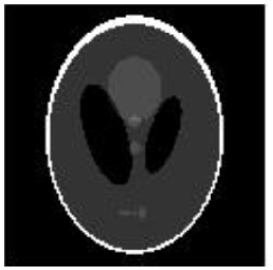
(a) Modulus of RPP

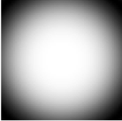
(b) $\rho={3\over 25\pi}\approx 0.038$

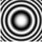
(c) $\rho={6\over 5\pi}\approx 0.38$

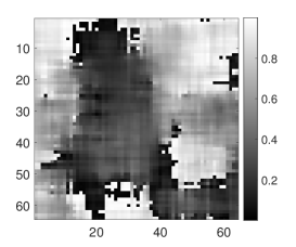
(d) $\ell=16,m=64$

(e) $\ell=8,m=32$

(f) $\ell=4,m=16$

Figure 2. (a) The modulus of $128\times 128$ RPP; (b)&(c) The modulus of the real part of the respective Fresnel masks; (d), (e)&(f) The phases of various correlated random masks in the unit of $2\pi$.

A primary purpose of our numerical experiments is to find out how $q$ affects the numerical reconstruction and propose a practical guideline for using the minimalist scheme. We also want to see how the complexities of the mask and the object affect numerical performance. Finally, we want to test how robust the minimalist scheme is with respect to measurement noise.

As pointed out above, DR has the true solution as the unique fixed point in the object domain (Proposition 3.1) while AP has a better convergence rate than DR (Theorem 3.4). A natural way to combine their strengths is to use DR as the initialization method for AP. We choose AP and DR as the building blocks of our reconstruction algorithm because of the fixed point and convergence properties and also because there are no adjustable parameters which can be tuned to optimize the performance as in other algorithms [29, 14]. We do not claim that this combination yields the best algorithm for ptychography. Quite the contrary, our approach can be easily improved, for example, by initializing AP with the DR iterate of the least residual within a given number of iterations instead of the last iterate.

Our test image $f$ is randomly phased phantom (RPP): the phantom (Fig. 1 (a)) with phase at each pixel being independent and uniformly distributed over a specific range, referred to as the angle range hereafter. RPP is chosen for two reasons: (i) the core image is surrounded by dark pixels and the loose support makes RPP more challenging to reconstruct than an image of a tight support; (ii) the adjustable angle range is a convenient way for controlling the object complexity.

We use the relative error (RE) and residual (RR) as figures of merit for the recovered image $\hat{f}$:

$$\mbox{\rm RE}(\hat{f}) = \min_{\alpha\in\mathbb{R}}\frac{\|f-e^{i\alpha}\hat{f}\|}{\|f\|}$$

$$\mbox{\rm RR}(\hat{f}) = \frac{\|\ b-|A^{*}\hat{f}|\ \|}{\|b\|}.$$

5.1. Random and Fresnel masks

We consider two kinds of random masks $e^{{\rm i}\theta({\mathbf{n}})}$ where $\theta({\mathbf{n}})$ are either independent, identically distributed (i.i.d.) or $\ell$-correlated uniform random variables on $[0,2\pi]$, where $\ell\in\mathbb{N}$ is the correlation length.

The correlated random mask is produced by convolving the i.i.d. mask with the characteristic function of the set $\{(k_{1},k_{2})\in\mathbb{Z}^{2}:|\max\{|k_{1}|,|k_{2}|\}|\leq\ell/2\}$ and normalizing pixel-by-pixel to get a phase mask. The i.i.d. mask corresponds to $\ell=1$.

We also consider the Fresnel mask with

(75) $$\mu^{0}(k_{1},k_{2}):=\exp\left\{{\rm i}\pi\rho((k_{1}-\beta_{1})^{2}+(k_{2}-\beta_{2})^{2})/m\right\},\quad k_{1},k_{2}=1,\cdots,m\leavevmode\nobreak\ (={2n/q})$$

where $\rho,\beta_{1},\beta_{2}\in\mathbb{R}$ are adjustable parameters, as well as the plain mask ($\rho=0$). The choice of $\beta_{1},\beta_{2}$ has an insignificant effect on numerical reconstruction. The form of the discrete Fresnel phase is dictated by our goal of keeping the angular aperture of the illumination fixed independent of $m$ since (75) describes a point-source illumination with both the aperture (i.e. the linear size of the mask) and the distance to the object proportional to the parameter $m$ [1]. If we set the distance from the point source to the object to be $mL$ and the pixel size to be $\delta\times\delta$, then in the Fresnel kernel $\rho=\delta^{2}/(\lambda L)$ where $\lambda$ is the wavelength. For a different $\rho$, we imagine varying $L$ while keeping $\lambda$ and $\delta$ fixed. The larger $L$ is, the smaller $\rho$ is and hence the coarser the mask is. With the minimalist scheme described in Section 1.2 and the Fresnel mask (75) with $\rho$ fixed, the total bandwidth of the mask and the total number of measurement data are fixed as $q$ varies. Fig. 2(b)(c) shows the real part of the Fresnel mask at two different $\rho$.

In the same spirit, in the case of random mask, we let the correlation length $\ell$ be proportional to $m$ as $q$ varies when we turn to the noisy case. Fig. 2(d)-(f) shows three examples of correlated masks with the same ratio $m/\ell=4$.

5.2. Twin images with the Fresnel mask

Our first experiment has to do with the choice of the Fresnel parameter $\rho$ in (75). Fig. 3 shows that the error spikes around $\rho\in\mathbb{N}$. This phenomenon is due to the existence of twin-like image. As explained in the appendix, for $q=2$, $g:=Qf\odot Q\mu\odot\overline{\mu}$ produces the same ptychographic data as $f$ where $Q$ is the conjugate inversion operation. In such a case, ptychographic solutions are not unique and the ambiguity hurts the performance of reconstruction. For $q>2$, the spikes are much smaller than those of $q=2$. As $q$ increases from 2 to 6, the order of magnitude of fluctuation from peak to valley decreases from more than four orders of magnitude to about two or less. To avoid the twin-image ambiguity, we choose irrational values of $\rho$.

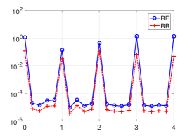
(a) $q=2$

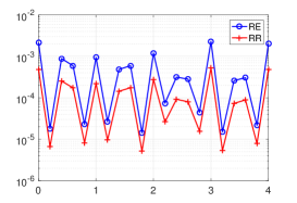
(b) $q=4$

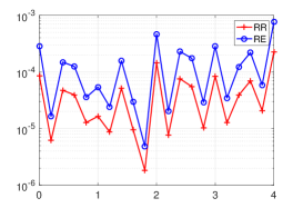
(c) $q=6$

Figure 3. RE and RR on the semi-log scale versus the parameter $\rho$ of the Fresnel mask with 200 FDR iterations followed by 100 AP iterations for $60\times 60$ RPP of the full angle range $[0,2\pi]$.

5.3. Effect of the mask

Fig. 4 shows RE versus 100 AP iterations after the DR initialization with the i.i.d. mask and two Fresnel masks for RPP of various angle ranges (legend). We see that the i.i.d. mask produces the best initialization and the fastest convergence rate and that the Fresnel mask of a larger $\rho$ produces a better initialization and a better convergence rate than the Fresnel mask of a smaller $\rho$ for all angle ranges.

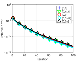
(a) i.i.d. mask

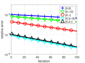
(b) Fresnel mask with $\rho=\frac{6}{5\pi}$

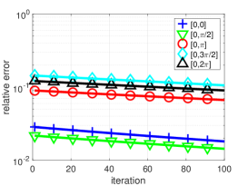
(c) Fresnel mask with $\rho=\frac{3}{25\pi}$

Figure 4. RE on the semi-log scale for $60\times 60$ RPP of various angle ranges (legend) versus 100 AP iterations with initialization given by 300 DR iterations with $q=4$.

5.4. Effect of $q$

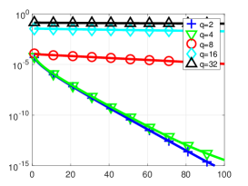
(a) i.i.d. mask

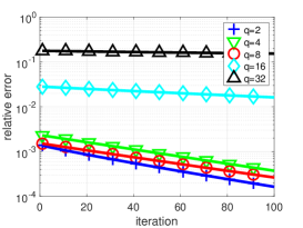
(b) Fresnel mask with $\rho={6\over 5\pi}$

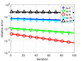
(c) Fresnel mask with $\rho={3\over 25\pi}$

Figure 5. RE on the semi-log scale for the $128\times 128$ RPP of angle range $[0,2\pi]$ vs 100 AP iterations after initialization given by 300 DR iterations with various $q$.

Fig. 5 shows RE versus 100 AP iterations after the DR initialization with an i.i.d. random mask and two Fresnel masks with various $q$. Interestingly, we observe that a mask of higher complexity (random or larger $\rho$) works better with a smaller value of $q$. But $q$ is as large as $32$, the results are always poor.

5.5. Effect of noise

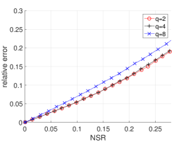
(a) Random with $50\%$ overlap

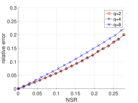
(b) Fresnel with $\rho={6\over 5\pi}$

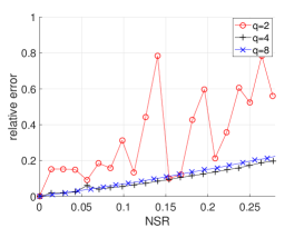
(c) Fresnel with $\rho={3\over 25\pi}$

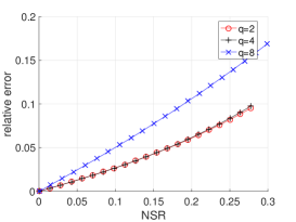
(d) Random with $75\%$ overlap

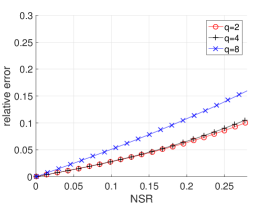
(e) Fresnel with $\rho={6\over 5\pi}$

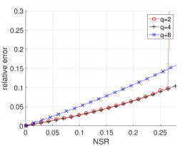
(f) Fresnel with $\rho={3\over 25\pi}$

Figure 6. RE vs. NSR after 300 FDR iterations followed by 200 AP iterations for $64\times 64$ RPP of angle range $[0,2\pi]$ with (a)-(c) $50\%$ and (d)-(f) $75\%$ overlap between adjacent masks.

To introduce both phase and magnitude noises to our signal model, we add complex Gaussian noise to $A^{*}f$ before taking the modulus as data

$$b=\left|A^{*}f+z\right|$$

where $z\in\mathbb{C}^{N}$ is an i.i.d. circularly symmetric complex Gaussian random vector. The size of the noise is measured in terms of the noise-to-signal ratio (NSR)

(76) $$\mbox{\rm NSR}=\frac{\|b-|A^{*}f|\|}{\|A^{*}f\|}$$

We also test the effect of increasing the overlap of adjacent masks from $50\%$ to $75\%$: With the same relation $m=2n/q$, $75\%$ overlap between adjacent masks corresponds to $4q^{2}$ diffraction patterns.

Fig. 6 shows RE versus NSR for various masks and $q$ with (top) $50\%$ and (bottom) $75\%$ overlap. The correlated masks used are shown in Fig. 2 (d)-(f) with $m/\ell=4$ so that the complexity of the mask is independent of $q$.

For up to $25\%$ NSR, the RE-NSR curves in Fig. 6 are roughly straight lines of a slope less than 1, with $q=4$ the best performing value across the board. The violent fluctuations in (c) for $q=2$ indicates non-convergent behaviors consistent with Fig. 5(c) with $q=2$.

Fig. 6(d)-(f) shows that the four times number of data with $75\%$ overlap predictably result in a significantly reduced RE, especially for $q=2,4$.

6. Conclusion and discussion

In the present work, we have proved the uniqueness theorem (Theorem 2.3, Corollary 2.4) for any ptychographic scheme with an independent random masks under the minimum overlap condition (16). We have also given a local geometric convergence analysis for AP and DR algorithms (Theorem 3.4). We have shown that DR has a unique fixed point in the object domain (Proposition 3.1) and given a simple criterion for distinguishing the true solution among possibly many fixed points of AP (Proposition 3.3). We chose AP and DR as the building blocks of our reconstruction algorithm because of the fixed point and convergence properties and because there are no adjustable parameters which can be tuned to optimize the performance as in other algorithms [29, 14].

We have proposed a minimalist scheme parametrized by $q=2n/m$ where $m$ is the number of mask pixels in each direction and given a lower bound on the geometric rate of convergence (Proposition 4.1). The bound $\gamma>1-C/q^{2}$ predicts a poor performance for the minimalist scheme with large $q$ which is confirmed by our numerical experiments.

In addition, we have performed extensive numerical experiments to find out what the general features of a well-performing mask are like, what the best-performing values of $q$ for a given mask are, how robust the minimalist scheme is with respect to measurement noise and what the significant factors affecting the noise stability are.

From our numerical experiments, we have found that (i) the mask of higher complexity (e.g. random masks or the Fresnel mask of a larger $\rho$) produces faster convergence in reconstruction than the mask of lower complexity (e.g. the Fresnel mask of a smaller $\rho$); (ii) the best-performing value of $q$ for a mask of higher complexity is smaller than that for a mask of lower complexity; (iii) ptychographic reconstruction with medium values of $q$ (e.g. $q\in[4,8]$) is robust with respect to measurement noise regardless of the mask used, with the ratio of RE to NSR less than unity; (iv) increased overlap between adjacent masks generally reduces the reconstruction error as expected.

We have not addressed an important potential of ptychography for retrieving the mask and the object simultaneously without knowing precisely the mask function (blind ptychography). We have previously proved the simultaneous determination of a roughly known mask and the object for a nonptychographic setting [9]. As a ptychographic reconstruction offers extra potential beyond a nonptychographic one, we will turn to blind ptychography in a forthcoming paper.

Appendix A Twin image with a Fresnel mask

We give a sufficient condition for the existence of twin image with the Fresnel masks that satisfies the symmetry of conjugate inversion, which we believe explain the poor performance of Fig. 5 (right column) for $c=0$ and spikes in Fig. 3 both for $q=2$.

Let $Q_{m}x$ be the conjugate inversion of $x\in\mathbb{C}^{m\times m}$, i.e. $(Q_{m}x)_{ij}=\overline{x}_{m+1-i,m+1-j}.$ For an even integer $m$, write

$$x=\left[\begin{matrix}x_{1}&x_{2}\\ x_{3}&x_{4}\end{matrix}\right],\quad x_{j}\in\mathbb{C}^{m/2\times m/2},\quad j=1,2,3,4,$$

and we have

$$Q_{m}x=\left[\begin{matrix}Q_{m/2}x_{4}&Q_{m/2}x_{3}\\ Q_{m/2}x_{2}&Q_{m/2}x_{1}\end{matrix}\right].$$

For ease of notation, we will omit writing the subscript in $Q$.

Proposition A.1.

Let $\rho\in\mathbb{Z}$ and $\mu\in\mathbb{C}^{m\times m}$ be the Fresnel mask with the elements

(77) $$\mu^{0}(k_{1},k_{2})=\exp\left\{{\rm i}\pi\rho((k_{1}-\beta_{1})^{2}+(k_{2}-\beta_{2})^{2})/m\right\},\quad k_{1},k_{2}=1,\ldots,m.$$

For an even integer $m$, the matrix

(80) $$\overline{Q\mu}\odot\mu:=\left(\begin{array}[]{ccc}h_{1}&h_{2}\\ h_{3}&h_{4}\end{array}\right),\quad h_{j}\in\mathbb{C}^{m/2\times m/2},\quad j=1,2,3,4,$$

satisfies the symmetry

(81) $$h_{1}=h_{4}=\gamma h_{2}=\gamma h_{3},\;\gamma=(-1)^{\rho+2cm}.$$

Proof.

With

(84) $$\mu=\left(\begin{array}[]{cc}\mu_{1}&\mu_{2}\\ \mu_{3}&\mu_{4}\end{array}\right),\quad\mu_{j}\in\mathbb{C}^{m/2\times m/2},\quad j=1,2,3,4,$$

we have

$$\overline{Q\mu}\odot\mu=\left[\begin{matrix}\overline{Q\mu_{4}}\odot\mu_{1}&\overline{Q\mu_{3}}\odot\mu_{2}\\ \overline{Q\mu_{2}}\odot\mu_{3}&\overline{Q\mu_{1}}\odot\mu_{4}\end{matrix}\right]$$

Direct algebra with (77) and $\rho\in\mathbb{Z}$ gives

$$\mu_{4}\odot\overline{Q\mu_{1}}=\mu_{2}\odot\overline{Q\mu_{3}}\exp\{(\rho+2cm)\pi{\rm i}\}=\mu_{3}\cdot\overline{Q\mu_{2}}\exp\{(\rho+2mc)\pi{\rm i}\}=\mu_{1}\cdot\overline{Q\mu_{4}}$$

and hence the desired result. ∎

Let $\Phi$ be the oversampled Fourier matrix as before. Note that the oversampled Fourier magnitude has the symmetry of conjugate inversion:

(85) $$|\Phi x|=|\Phi Qx|,\quad\forall x\in\mathbb{C}^{m\times m}.$$

Proposition A.2.

Let $q=2$ (hence $m=2n/q=n$). Suppose $\mu$ satisfies the symmetry (80)-(81). Let $h$ be the matrix given in (80). For any $x\in\mathbb{C}^{m\times m}$, let

$$y=Qx\odot\overline{h}.$$

Then $y$ and $x$ produce the same ptychographic data for $q=2$ with the mask $\mu$.

Proof.

We can write

$$y=\alpha\left[\begin{array}[]{cc}Qx_{4}\odot\overline{h_{1}}&Qx_{3}\odot\overline{h_{2}}\\ Qx_{2}\odot\overline{h_{3}}&Qx_{1}\odot\overline{h_{4}}\end{array}\right].$$

Let $R_{1}$ and $R_{2}$ be the reflectors defined by

$$R_{1}x=\left[\begin{array}[]{cc}x_{2}&x_{1}\\ x_{4}&x_{3}\end{array}\right],\quad R_{2}x=\left[\begin{array}[]{cc}x_{3}&x_{4}\\ x_{1}&x_{2}\end{array}\right],$$

for all $x\in\mathbb{C}^{m\times m}$. Let

$$y^{\prime} = (QR_{1}x)\odot\overline{R_{1}h},$$

$$y^{\prime\prime} = (QR_{2}x)\odot\overline{R_{2}h},$$

$$y^{\prime\prime\prime} = (QR_{2}R_{1}x)\odot\overline{R_{2}R_{1}h}.$$

We have from direct calculation that

$$|\Phi(x\odot\mu)| = |\Phi(y\odot\mu)|,$$

$$|\Phi(R_{1}x\odot\mu)| = |\Phi(y^{\prime}\odot\mu)|,$$

$$|\Phi(R_{2}x\odot\mu)| = |\Phi(y^{\prime\prime}\odot\mu)|,$$

$$|\Phi(R_{2}R_{1}x\odot\mu)| = |\Phi(y^{\prime\prime\prime}\odot\mu)|.$$

Proposition A.1 implies

(86) $$h=\gamma R_{1}h=\gamma R_{2}h=R_{2}R_{1}h=\mu\odot\overline{Q\mu}.$$

Using (85) and (86) we have

(87) $$|\Phi(x\odot\mu)|=|\Phi(Qx\odot Q\mu)|=|\Phi(Q(x)\odot\overline{h}\odot\mu)|=|\Phi(y\odot\mu)|.$$

Similarly, we have

(88) $$|\Phi(R_{1}x\odot\mu)|=|\Phi(QR_{1}x\odot Q\mu)|=|\Phi(QR_{1}x\odot\overline{\gamma R_{1}h}\odot\mu)|=|\Phi(y^{\prime}\odot\mu)|,$$

(89) $$|\Phi(R_{2}x\odot\mu)|=|\Phi(QR_{2}x\odot Q\mu)|=|F(QR_{2}x\odot\overline{\gamma R_{2}h}\odot\mu)|=|\Phi(y^{\prime\prime}\odot\mu)|,$$

(90) $$|\Phi(R_{2}R_{1}x\odot\mu)|=|\Phi(QR_{2}R_{1}\odot Q\mu)|=|\Phi(QR_{2}R_{1}x\odot\overline{R_{2}R_{1}h}\odot\mu)|=|\Phi(y^{\prime\prime\prime}\odot\mu)|.$$

The lefthand and righthand sides of eq. (87)-(90) are precisely the ptychographic data for $q=2$ with the mask $\mu$. ∎

Acknowledgements. The research of A. Fannjiang is supported in part by the US National Science Foundation grant DMS-1413373.

References

- [1] M. Born and E. Wolf, Principles of Optics, 7-th edition, Cambridge University Press, 1999 (pages 199-201).
- [2] O. Bunk, M. Dierolf, S. Kynde, I. Johnson, O. Marti, F. Pfeiffer, “Influence of the overlap parameter on the convergence of the ptychographical iterative engine,” Ultramicroscopy 108 (5) (2008) 481-487.
- [3] Chapman, H. N. ”Microscopy: A new phase for X-ray imaging”. Nature. 467 (2010), 409-410.
- [4] P. Chen and A. Fannjiang, “Phase retrieval with a single mask by Douglas-Rachford algorithms,” Appl. Comput. Harmon. Anal. 2016, http://dx.doi.org/10.1016/j.acha.2016.07.003.
- [5] P. Chen, A. Fannjiang and G. Liu, “Phase retrieval with one or two coded diffraction patterns by alternating projection with the null initialization,” J. Fourier Anal. Appl. 2017, DOI 10.1007/s00041-017-9536-8.
- [6] M. Dierolf, A. Menzel, P. Thibault, P. Schneider, C. M. Kewish, R. Wepf, O. Bunk, and F. Pfeiffer, “ Ptychographic x-ray computed tomography at the nanoscale,” Nature 467 (2010), 436-439.
- [7] A. Fannjiang, “Absolute uniqueness of phase retrieval with random illumination,” Inverse Problems 28 (2012), 075008 (2012).
- [8] A. Fannjiang and W. Liao, “Phase retrieval with random phase illumination,” J. Opt. Soc. A 29 (2012), 1847-1859.
- [9] A. Fannjiang and W. Liao, “Fourier phasing with phase-uncertain mask,” Inverse Problems 29 (2013) 125001.
- [10] H.M.L. Faulkner and J.M. Rodenburg, “Movable aperture lensless transmission microscopy: A novel phase retrieval algorithm,” Phys. Rev. Lett.93:2 (2004), 023903.
- [11] H.M.L. Faulkner and J.M. Rodenburg, “Error tolerance of an iterative phase retrieval algorithm for moveable illumination microscopy,” Ultramicroscopy 103:2 (2005), 153-164.
- [12] Guizar-Sicairos, M. & Fienup, J. R. “Phase retrieval with transverse translation diversity: a nonlinear optimization approach.” Opt. Express 16 (2008), 7264-7278.
- [13] Hayes, M. “The reconstruction of a multidimensional sequence from the phase or magnitude of its Fourier transform,” IEEE Trans. Acoust. Speech Signal Process. 30 (1982), 140-154.
- [14] R. Hesse, D. R. Luke, S. Sabach, and M.K. Tam, “Proximal heterogeneous block implicit-explicit method and application to blind ptychographic diffraction imaging,” SIAM J. Imag. Sci. 8 (2015) pp. 426-457.
- [15] Hoppe, W. ”Beugung im inhomogenen Prim rstrahlwellenfeld. I. Prinzip einer Phasenmessung von Elektronenbeungungsinterferenzen”. Acta Crystallographica Section A. 25 (4) (1969) 495.
- [16] Hoppe, W. “Beugung im inhomogenen Prim rstrahlwellenfeld. III. Amplituden- und Phasenbestimmung bei unperiodischen Objekten”, Acta Crystallographica Section A. 25 (4) (1969) 508.
- [17] J. Hunt, T. Driscoll, A. Mrozack, G. Lipworth, M. Reynolds, D. Brady, and D. R. Smith, ”Metamaterial Apertures for Computational Imaging,” Science 339 (2013), 310 313.
- [18] M. A. Iwen, A. Viswanathan, and Y. Wang, “Fast phase retrieval from local correlation measurements,” SIAM J. Imaging Sci. 9(4)(2016), pp. 1655-1688.
- [19] G. Lipworth, A. Mrozack, J. Hunt, D.L. Marks, T. Driscoll, D. Brady, ”Metamaterial apertures for coherent computational imaging on the physical layer,” J. Opt. Soc. Am. A 30 (2013), 1603 1612.
- [20] A. M. Maiden, M. J. Humphry, F. Zhang and J. M. Rodenburg, “Superresolution imaging via ptychography,” J. Opt. Soc. Am. A 28 (2011), 604-612.
- [21] Maiden, A. M. & Rodenburg, J. M. “An improved ptychographical phase retrieval algorithm for diffractive imaging.” Ultramicroscopy 109 (2009), 1256-1262.
- [22] A. M. Maiden, J. M. Rodenburg and M. J. Humphry, Optical ptychography: a practical implementation with useful resolution. Opt. Lett. 35 (2010), 2585-2587.
- [23] A.M. Maiden, G.R. Morrison, B. Kaulich, A. Gianoncelli & J.M. Rodenburg, “Soft X-ray spectromicroscopy using ptychography with randomly phased illumination,” Nat. Commun. 4 (2013), 1669.
- [24] J.M. Rodenburg and H.M.L. Faulkner, “A phase retrieval algorithm for shifting illumination”. Applied Physics Letters 85 (2004), 4795.
- [25] Y. S. G. Nashed, D. J. Vine, T. Peterka, J. Deng, R. Ross and C. Jacobsen, “Parallel ptychographic reconstruction,” Opt. Exp. 22 (2014) 32082-32097.
- [26] P. Thibault, M. Dierolf, A. Menzel, O. Bunk, C. David, F. Pfeiffer, “High-resolution scanning X-ray diffraction microscopy”, Science 321 (2008), 379-382.
- [27] P. Thibault, M. Dierolf, O. Bunk, A. Menzel, F. Pfeiffer, “Probe retrieval in ptychographic coherent diffractive imaging,” Ultramicroscopy 109 (2009), 338-343.
- [28] L. Tian, X. Li, K. Ramchandran and L. Waller, “Multiplexed coded illumination for Fourier Ptychography with an LED array microscope,” Biomed. Opt. Express 5(7) (2014): 2376-2389.
- [29] Z. Wen, C. Yang, X. Liu and S. Marchesini, “Alternating direction methods for classical and ptychographic phase retrieval,” Inverse Problems 28 (2012), 115010.
- [30] X. Zhang, J. Jiang, B. Xiangli, G.R. Arce, “Spread spectrum phase modulation for coherent X-ray diffraction imaging,” Optics Express 23 (2015), 25034-25047.
- [31] C. M. Watts, D. Shrekenhamer, J. Montoya, G. Lipworth, J. Hunt, T. Sleasman, S. Krishna, D. R. Smith, and W. J. Padilla, ”Terahertz compressive imaging with metamaterial spatial light modulators,” Nat. Photon. 8 (2014), 605-609.