Quantum Electron Plasma and Interaction of S-wave with Thin Metallic Film

Abstract

An interaction of electromagnetic S-wave with thin flat metallic film is numerically studied for the quantum degenerate electron plasma. One considers the reflectance, transmittance and absorptance power coefficients. A contribution of quantum wave properties of electrons to the power coefficients is shown in comparison of the coefficients with ones evaluated for both the classical spatial dispersion and the Drude – Lorentz approaches. This contribution is detected for the infrared and terahertz frequencies in case of nanoscale film width.

PACS numbers:   42.25.Bs, 78.20.-e, 78.66.Bz

Keywords:   quantum plasma, metallic film, optical coefficients

Introduction

At current time, a large attention pays to study of the interaction of electromagnetic waves with tiny or nanoscale metallic films [1] – [13]. Such researches have not only theoretical interest but aimed also on the practical applications in contemporary optical facilities. Investigations of the interaction widely exploit the kinetic Fermi – Dirac electron gas theory. The theory leads to the optical spatial dispersion property of the electron plasma. And consequently, a theory of interaction of the electromagnetic wave with the flat infinite metallic film when the conductivity electrons in metal reflect specularly from the borders of the film, was elaborated successfully [2, 3].

But such investigations almost always neglect the de Broglie, or quantum wave, properties of electrons in the electron plasma. The principal problem was in getting the correct dielectric functions, or permittivities, of the quantum electron plasma [6, 7], [15] – [18]. The most pragmatic way to obtain the functions is when one uses the Liouville – Schroedinger equation in the relaxation time approximation for the electron density matrix complying with conservation laws [19]. The second strong difficulty in the incorporation of the electron wave property into the electron plasma is an account for the various boundary conditions applied to the electron density matrix. The well-known specular-diffuse boundary conditions for the classical kinetic function are not transmitted straightforward to the density matrix owing to the uncertainty principle. Here, the Wigner function approaches the classical kinetic one, and common-type classical boundary conditions due to the Fourier transform are too complicate in case of quantum plasma (see also [20]).

However, the electrons in a metal obey the quantum laws. And therefore, the quantum wave electron effects should influence on light interaction with a metal. In the paper [21], the influence of the quantum wave effects of electron plasma on the interaction of P-wave with metallic film was shown in case of visible and ultraviolet light.

In this paper, we study the interaction of electromagnetic S-wave with quantum degenerate electron plasma in the thin flat metallic film placed between two transparent nonconducting media. We took for investigation the reflectance, transmittance and absorptance power coefficients. We consider the quantum degenerate electron plasma with invariable relaxation time in case of specular electron reflection from the film surface. The dielectric function (permittivity) of the quantum electron plasma is taken in the Mermin approach [7, 17]. We investigate the power coefficients as functions of frequency and of incidence angle. The evaluated coefficients are compared with those obtained both in case of the Drude – Lorentz theory without spatial dispersion and in case of the classical degenerate electron plasma approach when taking into account the spatial dispersion.

1 The model and the power coefficients

We consider the flat uniform metallic film of the thickness $d$ placed between two transparent dielectric media. These media supposed to be uniform, isotropic and nonmagnetic ones having the positive constant permittivities $\varepsilon_{1}$ and $\varepsilon_{2}$. Hence we neglect the light dispersion and absorption of the media. Let us suppose that the electromagnetic wave is incident from the first dielectric medium on the film under the angle $\theta$ from the surface normal (fig. 1). Then in case of a solid second medium, it can be treated as a substrate.

Let the $Z$ axis is directed orthogonally to the film surface towards the second dielectric medium. We took $z=0$ plane as the film surface contacting with first medium. And hence, the $z=d$ is the second film surface having contact with the second medium (fig. 1). Further, we take the $X$ axis lying both in the film surface and in the incidence plane towards the wave propagation. And at the end, the direction of the third $Y$ axis taken in such a way that the rectangular system is the right-handed one.

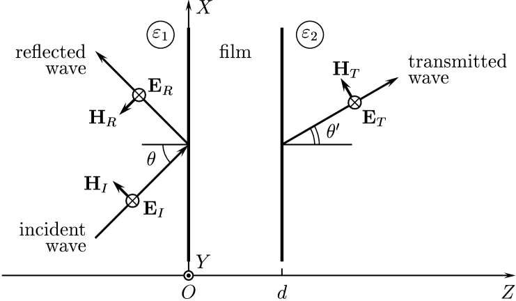
Fig. 1: The metallic film between two dielectric media with $\varepsilon_{1}$ and $\varepsilon_{2}$, and the incident, reflected and transmitted waves.

We study the S-waves when the ${\bf H}$ vectors of the waves incident on (${\bf H}_{I}$), reflected from (${\bf H}_{R}$) and transmitted through the film (${\bf H}_{T}$) lie in the incidence plane (see fig. 1). Then the ${\bf E}$ vectors of the waves (${\bf E}_{I}$, ${\bf E}_{R}$ and ${\bf E}_{T}$) are parallel to the $Y$ axis.

The electric and magnetic fields of the S-waves in the $z<0$ half-space projected onto $X$ and $Y$ axes look as [2, 22] (fig. 1)

$$\left\{\begin{array}[]{lll}E_{y}(x,y,z,t)&=&{\rm e}^{{\rm i}(k_{1x}x-\omega t)}\bigl{[}-a_{I}\,{\rm e}^{{\rm i}k_{1z}z}-a_{R}\,{\rm e}^{-{\rm i}k_{1z}z}\bigr{]},\\ H_{x}(x,y,z,t)&=&\displaystyle{\rm e}^{{\rm i}(k_{1x}x-\omega t)}\bigl{[}a_{I}\,{\rm e}^{{\rm i}k_{1z}z}-a_{R}\,{\rm e}^{-{\rm i}k_{1z}z}\bigr{]}\frac{\sqrt{\varepsilon_{1}}}{Z_{0}}\cos\theta.\end{array}\right.$$ (1)

In the $z>d$ half-space, the projections of these fields are the following:

$$\left\{\begin{array}[]{lll}E_{y}(x,y,z,t)&=&-{\rm e}^{{\rm i}(k_{2x}x-\omega t)}a_{T}\,{\rm e}^{{\rm i}k_{2z}(z-d)},\\ H_{x}(x,y,z,t)&=&\displaystyle{\rm e}^{{\rm i}(k_{2x}x-\omega t)}a_{T}\frac{\sqrt{\varepsilon_{2}}}{Z_{0}}\,{\rm e}^{{\rm i}k_{2z}(z-d)}\cos\theta^{\prime}.\end{array}\right.$$ (2)

Here $\omega$ is the wave frequency, $k_{1x}$ and $k_{1z}$ are the $x$- and $z$-projections of the incident wave vector ${\bf k}_{1}$ in the initial dielectric medium, $k_{2x}$ and $k_{2z}$ are the same coordinates of the transmitted wave vector ${\bf k}_{2}$ in the second dielectric medium:

$$k_{1x}=\frac{\omega}{c}\sqrt{\varepsilon_{1}}\sin\theta=k_{2x}=\frac{\omega}{c}\sqrt{\varepsilon_{2}}\sin\theta^{\prime};$$ (3)

$$k_{1z}=\frac{\omega}{c}\sqrt{\varepsilon_{1}}\cos\theta,\qquad k_{2z}=\frac{\omega}{c}\sqrt{\varepsilon_{2}}\cos\theta^{\prime}.$$

Further, the $a_{R}$, $a_{I}$ and $a_{T}$ stand for the complex electric field amplitudes of the incident, reflected and transmitted waves, respectively. The $c$ is the vacuum speed of light, $Z_{0}$ denotes the dimensional (in Ohm) vacuum impedance. And at the end, $\theta^{\prime}$ is the narrow refraction angle into the second dielectric medium from the surface normal (fig. 1). Note that in the case of total internal reflection when  $\sin\theta^{\prime}>1$,  the $\cos\theta^{\prime}$ value is pure imaginary. Then since the transmitted wave should not amplify infinitely, the sign of the imaginary value has to be positive i.e.  $\mathop{\rm Im}\nolimits\cos\theta^{\prime}>0$. Therefore, the $\cos\theta^{\prime}$ is evaluated according to the equation following from (3) one:

$$\cos\theta^{\prime}=\left\{\begin{array}[]{lll}\displaystyle\sqrt{1-\frac{\varepsilon_{1}}{\varepsilon_{2}}\sin^{2}\theta},&&\displaystyle\sin\theta\leqslant\sqrt{\frac{\varepsilon_{2}}{\varepsilon_{1}}};\\[10.00002pt] \displaystyle{\rm i}\sqrt{\frac{\varepsilon_{1}}{\varepsilon_{2}}\sin^{2}\theta-1},&&\displaystyle\sin\theta>\sqrt{\frac{\varepsilon_{2}}{\varepsilon_{1}}}.\end{array}\right.$$ (4)

In the film zone $0<z<d$, the electric and magnetic fields may be represented in the following way:

$$\left\{\begin{array}[]{lll}E_{y}(x,y,z,t)&=&{\rm e}^{{\rm i}(k_{1x}x-\omega t)}\bigl{[}\alpha_{1}E^{(1)}_{y}(z)+\alpha_{2}E^{(2)}_{y}(z)\bigr{]},\\ H_{x}(x,y,z,t)&=&{\rm e}^{{\rm i}(k_{1x}x-\omega t)}\bigl{[}\alpha_{1}H^{(1)}_{x}(z)+\alpha_{2}H^{(2)}_{x}(z)\bigr{]}.\end{array}\right.$$ (5)

Here $\alpha_{1}$ and $\alpha_{2}$ are some constant coefficients, and $E^{(j)}_{y}(z)$ and $H^{(j)}_{x}(z)$ stand for the antisymmetric or symmetric modes of electric and magnetic fields ($j=1,2$):

$$E^{(j)}_{y}(z)=(-1)^{j}E^{(j)}_{y}(d-z),\qquad H^{(j)}_{x}(z)=(-1)^{j+1}H^{(j)}_{x}(d-z).$$ (6)

The electric and magnetic fields on the film surfaces $z=0$ and $z=d$ have to satisfy the boundary conditions:

$$\left\{\begin{array}[]{lll}E_{y}(x,y,-0,t)&=&E_{y}(x,y,+0,t),\\ H_{x}(x,y,-0,t)&=&H_{x}(x,y,+0,t);\end{array}\right.$$ (7)

$$\left\{\begin{array}[]{lll}E_{y}(x,y,d-0,t)&=&E_{y}(x,y,d+0,t),\\ H_{x}(x,y,d-0,t)&=&H_{x}(x,y,d+0,t).\end{array}\right.$$ (8)

In order to connect the electric and magnetic fields on the film surfaces, it is convenient to use the dimensionless surface impedance [2] – [5]. For the S-wave modes on the $z=0$ surface, the impedance defined as ($j=1,2$):

$$Z^{(j)}_{S}=\frac{1}{Z_{0}}\frac{E^{(j)}_{y}(+0)}{H^{(j)}_{x}(+0)}.$$ (9)

Substituting (1) and (5) into (7), (2) and (5) into (8), employing the property (6) of the modes and using the surface impedance (9), after elimination of similar multipliers one gets the following system:

$$\left\{\begin{array}[]{rcl}-(a_{I}+a_{R})&=&\alpha_{1}E^{(1)}_{y}(+0)+\alpha_{2}E^{(2)}_{y}(+0),\\ (a_{I}-a_{R})\sqrt{\varepsilon_{1}}\cos\theta&=&\displaystyle\alpha_{1}\frac{E^{(1)}_{y}(+0)}{Z^{(1)}_{S}}+\alpha_{2}\frac{E^{(2)}_{y}(+0)}{Z^{(2)}_{S}},\\[10.00002pt] -a_{T}&=&-\alpha_{1}E^{(1)}_{y}(+0)+\alpha_{2}E^{(2)}_{y}(+0),\\ a_{T}\sqrt{\varepsilon_{2}}\cos\theta^{\prime}&=&\displaystyle\alpha_{1}\frac{E^{(1)}_{y}(+0)}{Z^{(1)}_{S}}-\alpha_{2}\frac{E^{(2)}_{y}(+0)}{Z^{(2)}_{S}}.\end{array}\right.$$ (10)

After elimination of the values $\alpha_{j}E^{(j)}_{y}(+0)$ ($j=1,2$) from the system (10), one comes to the system

$$\left\{\begin{array}[]{rcl}a_{T}&=&U^{(1)}_{S}a_{I}+V^{(1)}_{S}a_{R},\\ a_{T}&=&-U^{(2)}_{S}a_{I}-V^{(2)}_{S}a_{R}.\end{array}\right.$$ (11)

Here is denoted ($j=1,2$):

$$U^{(j)}_{S}=\frac{1+Z^{(j)}_{S}\sqrt{\varepsilon_{1}}\cos\theta}{1-Z^{(j)}_{S}\sqrt{\varepsilon_{2}}\cos\theta^{\prime}},\qquad V^{(j)}_{S}=\frac{1-Z^{(j)}_{S}\sqrt{\varepsilon_{1}}\cos\theta}{1-Z^{(j)}_{S}\sqrt{\varepsilon_{2}}\cos\theta^{\prime}}.$$ (12)

Let us turn now to the definition of the reflectance $R$, transmittance $T$ and absorptance $A$ power coefficients. The first two of them are the ratios [23, 22]:

$$R=\frac{|\langle S_{z}\rangle_{R}|}{|\langle S_{z}\rangle_{I}|},\qquad T=\frac{|\langle S_{z}\rangle_{T}|}{|\langle S_{z}\rangle_{I}|},$$ (13)

where $\langle S_{z}\rangle$ is the time averaged energy flux density, or Poynting, vector, projected onto the $Z$ axis:

$$\langle S_{z}\rangle=\frac{1}{2}\mathop{\rm Re}\nolimits({\bf E}\times{\bf H}^{*})\cdot{\bf e}_{z},$$ (14)

where ^∗ is the complex conjugation and ${\bf e}_{z}$ stands for the unit vector towards the $Z$ axis direction. The $I$, $R$ and $T$ subscript letters in the equations (13) stand for the respective incident, reflected and transmitted waves. The expression (14) for the S-wave can be transformed to the following one:

$$\langle S_{z}\rangle=-\frac{1}{2}\mathop{\rm Re}\nolimits(E_{y}H^{*}_{x}).$$ (15)

We substitute the equations (1) and (2) to the (15) and separate the terms related to $\langle S_{z}\rangle_{I}$, $\langle S_{z}\rangle_{R}$ and $\langle S_{z}\rangle_{T}$. Then we substitute these terms to the equations (13) and use the positivity of the dielectric constants $\varepsilon_{1}$ and $\varepsilon_{2}$. And one comes to the following expressions for the reflectance $R$ and transmittance $T$ power coefficients:

$$R=\left|\frac{a_{R}}{a_{I}}\right|^{2},\qquad T=\mathop{\rm Re}\nolimits\left(\frac{\cos\theta^{\prime}}{\cos\theta}\sqrt{\frac{\varepsilon_{2}}{\varepsilon_{1}}}\,\right)\left|\frac{a_{T}}{a_{I}}\right|^{2}.$$ (16)

Evaluating the ratios $a_{R}/a_{I}$ and $a_{T}/a_{I}$ from the system (11) and substituting them into the equations (16), one arrives at the final equations for the $R$, $T$ and also for the absorptance $A$:

$$R=\left|\frac{U^{(1)}_{S}+U^{(2)}_{S}}{V^{(1)}_{S}+V^{(2)}_{S}}\right|^{2},$$ (17)

$$T=\mathop{\rm Re}\nolimits\left(\frac{\cos\theta^{\prime}}{\cos\theta}\sqrt{\frac{\varepsilon_{2}}{\varepsilon_{1}}}\,\right)\left|\frac{U^{(1)}_{S}V^{(2)}_{S}-U^{(2)}_{S}V^{(1)}_{S}}{V^{(1)}_{S}+V^{(2)}_{S}}\right|^{2},$$ (18)

$$A=1-R-T.$$ (19)

The power coefficients (17) – (19) comply with those obtained in paper [14] for the S-wave. In the particular case when the dielectric media are vacuum or air with $\varepsilon_{1}=\varepsilon_{2}=1$, one has $\theta^{\prime}=\theta$ and the equations (17), (18) reproduce the reflectance and transmittance power coefficients presented in papers [3, 4, 5].

2 The surface impedance and the dielectric function of the degenerate electron plasma

The surface impedance defined by equation (9), was evaluated in [3] for the flat uniform metallic film with isotropic electron plasma in the case of specular electron reflections from the film borders. It can be rewritten in terms of dimensionless values and for the S-wave, it looks as follows ($j=1,2$):

$$Z^{(j)}_{S}=-\frac{2{\rm i}\Omega}{\beta W}\sum_{n}\frac{1}{\Omega^{2}\varepsilon_{tr}(\Omega,Q_{n})-(Q_{n}/\beta)^{2}},$$ (20)

where $\Omega$, $\beta$, $W$, $Q_{n}$, $Q_{x}$ are the dimensionless variables and parameters:

$$\Omega=\frac{\omega}{\omega_{p}},\qquad\beta=\frac{v_{F}}{c},\qquad W=\frac{\omega_{p}\,d}{v_{F}},$$ (21)

$$Q_{n}=\sqrt{\Bigl{(}\frac{\pi n}{W}\Bigr{)}^{2}+Q^{2}_{x}},\qquad Q_{x}=\frac{v_{F}k_{x}}{\omega_{p}}.$$ (22)

Here $\omega_{p}$ is the frequency of the degenerate electron plasma, $v_{F}$ is the electron Fermi velocity of conductivity electrons, the $k_{x}$ is the $x$-projection of the wave vector ${\bf k}$. Further, the $\varepsilon_{tr}(\Omega,Q)$ is the transverse dielectric function (permittivity) of the isotropic electron plasma. Summation in (20) is performed over all odd integers $n$ if $j=1$ or over all even integers if $j=2$:

$$\begin{array}[]{lll}j=1:&&n=\pm 1,\,\pm 3,\,\pm 5,\,\pm 7,\,\ldots;\\ j=2:&&n=0,\,\pm 2,\,\pm 4,\,\pm 6,\,\ldots.\end{array}$$

It is convenient to use dimensionless variables in the units of the degenerate electron plasma. The transverse dielectric function of the quantum electron plasma at zero temperature with invariable relaxation time owing to electron collisions, obtained in the Mermin approach involving the electron density matrix in the momentum space, looks as follows [7, 17]:

$$\varepsilon^{(qu)}_{tr}(\Omega,Q)=1-\frac{1}{\Omega^{2}}\left(1+\frac{\Omega G(\Omega+{\rm i}\gamma,Q)+{\rm i}\gamma G(0,Q)}{\Omega+{\rm i}\gamma}\right).$$ (23)

Here the function $G$ is defined by the equation:

$$G(\Omega+{\rm i}\gamma,Q) = \frac{3}{16r}\Bigl{[}B_{2}(\Omega_{+}+{\rm i}\gamma,Q)-B_{2}(\Omega_{-}+{\rm i}\gamma,Q)\Bigr{]}+$$

$$+ \frac{9}{8}\Bigl{(}\frac{\Omega+{\rm i}\gamma}{Q}\Bigr{)}^{2}+\frac{3}{32}(Qr)^{2}-\frac{5}{8},$$

where the functions and variables ($\alpha=1,2$)

$$B_{\alpha}(\Omega+{\rm i}\gamma,Q)=\frac{1}{Q^{2\alpha+1}}\bigl{[}(\Omega+{\rm i}\gamma)^{2}-Q^{2}\bigr{]}^{\alpha}\,L(\Omega+{\rm i}\gamma,Q),$$ (24)

$$L(\Omega+{\rm i}\gamma,Q)=\ln\frac{\Omega+{\rm i}\gamma-Q}{\Omega+{\rm i}\gamma+Q},$$ (25)

$$\Omega_{\pm}=\Omega\pm\frac{1}{2}Q^{2}r.$$

And further, the dimensionless variable and parameters

$$Q=\frac{v_{F}|{\bf k}|}{\omega_{p}},\qquad\gamma=\frac{1}{\omega_{p}\tau},\qquad r=\frac{\hbar\omega_{p}}{m_{e}v^{2}_{F}}.$$ (26)

Here $\tau$ is the relaxation time owing to the electron collisions, $m_{e}$ is the effective mass of the conductance electrons and $\hbar$ is the Planck constant.

The complex logarithm ratio $L(\Omega+{\rm i}\gamma,Q)$ defined by equation (25), has the branching real negative half-line on the complex plane $\Omega+{\rm i}\gamma$. Then one must evaluate the logarithm ratio using the prescription:

$$L(\Omega+{\rm i}\gamma,Q)=\frac{1}{2}\ln\frac{(\Omega-Q)^{2}+\gamma^{2}}{(\Omega+Q)^{2}+\gamma^{2}}+{\rm i}\left(\arctan\frac{\Omega+Q}{\gamma}-\arctan\frac{\Omega-Q}{\gamma}\right).$$ (27)

From (27) follows that the function $G(0,Q)$ is real since $Q\geqslant 0$ and $\gamma\geqslant 0$.

The transverse dielectric function (23) in the classical limit $r\to 0$ go over to corresponding dielectric function of the degenerate Fermi gas disregarding for the quantum wave electron properties called as classical spatial dispersion case [2, 13, 14]:

$$\varepsilon^{(cl)}_{tr}(\Omega,Q) = 1-\frac{3}{4\Omega}\Biggl{(}\frac{2(\Omega+{\rm i}\gamma)}{Q^{2}}+B_{1}(\Omega+{\rm i}\gamma,Q)\Biggr{)},$$ (28)

where the function $B_{1}(\Omega+{\rm i}\gamma,Q)$ is defined by the equation (24). And also in the infinite wavelength limit $Q\to 0$, both the quantum dielectric function (23) and the classical spatial dispersion one (28) go over to the classical Drude – Lorentz electron dielectric function without spatial dispersion [22]:

$$\varepsilon^{(DL)}_{tr}(\Omega)=1-\frac{1}{\Omega(\Omega+{\rm i}\gamma)}.$$ (29)

It worth noting that in the case of Drude – Lorentz dielectric function (29), one can perform exactly the summation in (20).

We return to the surface impedance (20). It is used in (12) to evaluate the power coefficients (17) – (19). The $Q_{x}$ variable in $Q_{n}$ is evaluated by substituting $k_{x}=k_{1x}$ by (3) in the (22) for $Q_{x}$ and using the definitions (21). Then one obtains:

$$Q_{x}=\Omega\beta\sqrt{\varepsilon_{1}}\sin\theta.$$ (30)

3 Numerical studies of the power coefficients for quantum electron plasma

We perform numerical investigation of the reflectance $R$, transmittance $T$ and absorptance $A$ power coefficients for S-wave in case of the quantum plasma. The coefficients are evaluated according to the equations (17) – (19) when one uses the formulas (4), (12), (20), (22) and (30) with the dielectric function (23). We study the coefficients as functions of variable $\Omega$ called by us as dimensionless frequency, and of the incidence angle $\theta$, for various film widths $d$ and for different surrounding dielectric media.

The initial data taken by us are characteristics of potassium [4]: $\omega_{p}=6.61\cdot{}10^{15}$ sec^-1,  $v_{F}=8.5\cdot{}10^{5}$ m/sec, the effective mass of conductance electron $m_{e}$ equals to the free electron mass, and the dimensionless parameter $\gamma=10^{-3}$. So taking into account (21) and (26), we have set the values $\beta=2.83\cdot{}10^{-3}$ and $r=1.07$.

Fig. 2: The reflectance $R$ (left plot) and absorptance $A$ (right plot) as functions of $\Omega$ for quantum plasma at $\beta=2.83\cdot{}10^{-3}$, $\gamma=10^{-3}$, $r=1.07$, $\theta=60^{\circ}$, $\varepsilon_{1}=1$ (air), $\varepsilon_{2}=2$ (quartz):  1 – $W=50$,  2 – $W=200$,  3 – $W=500$.

Typical results for $R$ and $A$ as functions of dimensionless frequency $\Omega$ for some values $W$ are shown at the fig. 2. The chosen values $W=50$, $200$ and $500$ correspond according to (21), to the film widths $d=6.43$ nm, $25.72$ nm and $64.3$ nm, respectively. The first surrounding medium is an air or vacuum with $\varepsilon_{1}=1$, and the second medium or substrate, is a quartz with $\varepsilon_{2}=2$. The considered frequency interval $10^{-3}\leqslant\Omega\leqslant{}2.5$ covers the ranges from the terahertz range to the ultraviolet one. One sees that almost always in the selected frequency interval, the reflectance $R$ and absorptance $A$ power coefficients decrease with growth of frequency. And also, a decrease of the power coefficients becomes less sharp with an increase of the film width $d$.

Fig. 3: The reflectance $R$ (left plot) and absorptance $A$ (right plot) as functions of $\Omega$ for quantum plasma at $\beta=2.83\cdot{}10^{-3}$, $\gamma=10^{-3}$, $r=1.07$, $\theta=60^{\circ}$, $W=50$, $\varepsilon_{1}=1$ (air):   1 – $\varepsilon_{2}=2$ (quartz),  2 – $\varepsilon_{2}=8$ (mica),  3 – $\varepsilon_{2}=40$ (technical ceramics).

Further, in the fig. 3 we show the coefficients $R$ and $A$ as functions of $\Omega$ for various second media, or substrates: a quartz with $\varepsilon_{2}=2$, a mica with $\varepsilon_{2}=8$, and a technical ceramics with $\varepsilon_{2}=40$. It is seen that within the considered frequency interval, both the reflectance $R$ and absorptance $A$ coefficients decrease with $\Omega$ growth. And the reflectance coefficient at the values $\Omega\gtrsim{}0.1$ — $0.25$ almost goes to a saturation. But if the absorptance decreases more strong at increase of the dielectric constant $\varepsilon_{2}$ of the second medium, the reflectance vice versa, decrease more gentle sloping.

And at the end of the section, we studied the power coefficients as functions of the incidence angle $\theta$. Typical results are presented at the fig. 4 for two film widths with $W=50$ and $W=500$. One sees that the reflectance $R$ almost always increases whereas the transmittance $T$ and absorptance $A$ decrease with growth of $\theta$.

Fig. 4: The coefficients $R$, $T$ and $A$ as functions of $\theta$ for quantum plasma at $\beta=2.83\cdot{}10^{-3}$, $\gamma=10^{-3}$, $r=1.07$, $\Omega=0.5$, $\varepsilon_{1}=1$, $\varepsilon_{2}=2$, $W=50$ (left plot), $W=500$ (right plot).

It worth to compare the results for S-wave with those in case of P-wave when the ${\bf E}$ vectors lie in the incidence plane, obtained in the quantum plasma approach [21]. The behavior of the power coefficients as functions of $\theta$ in case of S-wave is in somewhat reminiscent to the behavior for the P-wave. However in case of the P-wave, one observes resonant peaks of power coefficients in the region $\Omega\gtrsim{}1$. These peaks are caused by influence of longitudinal plasmons moving between borders of the metallic film [3, 11]. But here for the S-wave, these oscillations do not occur because the ${\bf E}$ vectors are parallel to film borders. And hence, one observes a smooth behavior of the power coefficients.

4 Comparison with classical spatial dispersion and Drude – Lorentz approaches

Now let us compare the results for S-wave in case of quantum plasma with those obtained for the classical spatial dispersion plasma and in case of Drude – Lorentz approach. To evaluate the power coefficients in the latter approaches, one employs again the equations (17) – (19) with (4), (12), (20), (22) and (30). But now the dielectric function (23) of the quantum plasma is replaced either by (28) or by (29) one.

Fig. 5: The reflectance $R$ (left plots) and absorptance $A$ (right plots) as functions of $\Omega$ at $\beta=2.83\cdot{}10^{-3}$, $\gamma=10^{-3}$, $r=1.07$, $\theta=60^{\circ}$, $\varepsilon_{1}=1$, $\varepsilon_{2}=2$, $W=200$ (upper plots), $W=1000$ (lower plots):   1 – quantum plasma (solid line),  2 – classical spatial dispersion case (dashed line),  3 – Drude – Lorentz approach (dotted line).

The numerical studies have shown that for the frequencies $\Omega\gg\pi/W$ (or $\omega\gg\pi{}v_{F}/d$), the power coefficients $R$, $T$ and $A$ for quantum plasma almost coincide with those in cases of both the classical spatial dispersion plasma and the Drude – Lorentz approach. So the results for the quantum plasma presented at the figs. 2 – 4, are valid also in cases of the classical and the Drude – Lorentz approaches for the frequencies $\Omega\gtrsim{}0.1$. However for the frequencies $\Omega\sim\pi/W$ ($\omega\sim\pi{}v_{F}/d$) when the film width satisfies the condition $W\gtrsim\beta^{-1}$ ($d\gtrsim{}c/\omega_{p}$), one observes a difference of the power coefficients evaluated for various approaches. Typical results illustrating such a disagreement are presented at the fig. 5 for the values $W=200$ and $1000$ ($d=25.72$ nm and $128.6$ nm). One sees that the deviation is the most visible for the absorptance $A$ and is more clear for large values $W$. Hence for these frequencies, both the quantum wave and the spatial dispersion effects of degenerate electron plasma contribute to interaction of the plasma with electromagnetic wave.

Fig. 6: The reflectance $R$ (left plot) and absorptance $A$ (right plot) as functions of $\theta$ at $\beta=2.83\cdot{}10^{-3}$, $\gamma=10^{-3}$, $r=1.07$, $\Omega=\pi/W$, $\varepsilon_{1}=1$, $\varepsilon_{2}=2$, $W=1000$:   1 – quantum plasma (solid line),  2 – classical spatial dispersion case (dashed line),  3 – Drude – Lorentz approach (dotted line).

The disagreement of various approaches is shown also at the fig. 6 for reflectance $R$ and absorptance $A$ as functions of incidence angle $\theta$, evaluated at the frequency $\Omega~{}=~{}\pi/W$. One sees the difference at small incidence angle. And the results for the classical spatial dispersion plasma deviate from the Drude – Lorentz approach stronger than for the quantum plasma. But when the $\theta$ increases to $90^{\circ}$, the disagreement decreases and vanishes.

These results agree with the data presented in the papers [5, 12] in cases of the classical spatial dispersion and the Drude – Lorentz approaches. The disagreement of various approaches takes place for the frequencies $\omega$ covering the terahertz and infrared ranges. As it was shown in [5], the difference of the spatial dispersion dielectric functions from the Drude – Lorentz one for the frequencies $\omega\sim\pi{}v_{F}/d$ is a manifestation of the resonance at the frequency of the periodic motion of electrons across the film between its borders which is just equal to $\pi{}v_{F}/d$. And also, a difference of the approaches is the most visible just for the absorptance $A$ when the film width $d\gtrsim{}c/\omega_{p}$ since the electromagnetic wave is well damped beyond the skin depth $c/\omega_{p}$.

The discrepancy of the power coefficients can be explained also by a contribution of the values $Q_{n}$ by (22) to the surface impedance (20) in cases of the quantum and classical spatial dispersion dielectric functions (23) and (28), for the values $n\sim{}1$ (see [12]). First of all, for the values $W\gtrsim\beta^{-1}$, a contribution of first terms with $n\neq{}0$ to (20) is essential. Further for the values $\Omega\sim\pi{}n/W\sim{}Q_{n}$ in case of small $n$ numbers, one has a deviation of both the quantum and the classical spatial dispersion transverse dielectric functions from the Drude – Lorentz one owing to smoothed critical behavior of functions (24).

Fig. 7: The ratios $|\varepsilon^{(qu)}_{tr}/\varepsilon^{(DL)}_{tr}|$ (left plot) and $|\varepsilon^{(cl)}_{tr}/\varepsilon^{(DL)}_{tr}|$ (right plot) as functions of $\Omega$ with $Q=Q_{n}$ at $\beta=2.83\cdot{}10^{-3}$, $\gamma=10^{-3}$, $r=1.07$, $\theta=60^{\circ}$, $\varepsilon_{1}=1$, $W=1000$:   1 – $n=1$ (solid line),  2 – $n=2$ (dashed line),  3 – $n=3$ (dotted line).

At the fig. 7, such a deviation is demonstrated for the magnitudes of the dielectric functions. We present the values $|\varepsilon^{(qu)}_{tr}/\varepsilon^{(DL)}_{tr}|$ and $|\varepsilon^{(cl)}_{tr}/\varepsilon^{(DL)}_{tr}|$ as functions of $\Omega$ with $Q=Q_{n}$ by (22) where $Q_{x}$ is evaluated according to (30), for first three values $n$. One sees that the extremes (maxima) of the ratios take place in the points $\Omega\simeq\pi{}n/W$. And in the vicinity of these extremal values, the ratios differ from the $1$. It can be seen also that the quantum dielectric function differs from the classical spatial dispersion one in the considered frequency region. Such a difference is caused by a contribution of the values $rQ^{2}_{n}/2$ and therefore, is explained by the influence of the quantum wave properties of the electrons on the dielectric function.

Conclusion

In the paper, we have investigated numerically an interaction of the electromagnetic S-wave with thin flat metallic film placed between two dielectric media, in the framework of the quantum degenerate electron plasma approach. We have selected for investigation the reflectance, transmittance and absorptance power coefficients. We have taken the transverse dielectric function of the quantum degenerate electron plasma with constant relaxation time in the Mermin approach in case of specular reflection of electrons from the film borders. The power coefficients were studied as functions of the frequency or the incidence angle at various nanoscale widths of the film and various second transparent media or substrate materials. The obtained results for the power coefficients of the quantum plasma were compared with the coefficients evaluated both in the classical spatial dispersion plasma and in the Drude – Lorentz approach without spatial dispersion.

It was shown that in the wide frequency interval from the terahertz range to ultraviolet one, the power coefficients of the quantum plasma have a smooth behavior without critical peaks. Further, dependence of the coefficients on the incidence angle in case of S-wave is reminiscent to the dependence in the P-wave case. And also for the large enough frequencies, the S-wave power coefficients of the quantum plasma almost coincide with the coefficients in cases of both the classical spatial dispersion plasma and the Drude – Lorentz approach. But for small frequencies lying in the terahertz and infrared ranges, the power coefficients evaluated in cases of various approaches differ from each other at the nanoscale width of the film. The origin of such a disagreement of the power coefficients was discussed. A discrepancy of the power coefficients indicates a manifestation of both the quantum wave property of electrons in plasma and the dimensional effects of interaction the electromagnetic wave with plasma due to the spatial dispersion.

The obtained results should be used in the theoretical studies of the quantum plasma as well as the interaction of the electromagnetic wave with nanoscale conducting objects. The results may have also a practical application in case of creation and use of optical instruments having thin metallic material.

This work is supported by the Research Grant of the President of Russian Federation  MK-7359-2016-9  and by the RFBR Grants  14-07-90009 Bel_a,  14-47-03608 r_centr_a.

References

- 1. Fuchs R., Kliewer K. L. and Pardee W. J., Phys. Rev., 150(2), 589–596 (1966).
- 2. Kliewer K. L. and Fuchs R., Phys. Rev., 172(3), 607–624 (1968).
- 3. Jones W. E., Kliewer K. L. and Fuchs R., Phys. Rev., 178(3), 1201–1203 (1969).
- 4. Kliewer K. L. and Fuchs R., Phys. Rev., 185(3), 905–913 (1969).
- 5. Kliewer K. L. and Fuchs R., Phys. Rev. B, 2(8), 2923–2936 (1970).
- 6. Lindhard J., Danske Vid. Selsk. Mat.-Fys. Medd., 28(8), 1–57 (1954).
- 7. Mermin N. D., Phys. Rev. B, 1(5), 2362–2363 (1970).
- 8. Latyshev A. V. and Yushkanov A. A., Comput. Math. and Math. Phys., 33(2), 229–239 (1993).
- 9. Latyshev A. V., Lesskis A. G. and Yushkanov A. A., Theor. and Math. Phys., 90(2), 119–126 (1992).
- 10. Sondheimer E. H., Advances in Physics, 50(6), 499–537 (2001).
- 11. Pitarke J. M., Silkin V. M., Chulkov E. V. and Echenique P. M., Rep. Prog. Phys., 70, 1–87 (2007).
- 12. Paredez-Juarez A., Diaz-Monge F., Makarov N. M. and Perez-Rodriguez F., JETP Letters, 90(9), 623–627 (2009).
- 13. Latyshev A. V. and Yushkanov A. A., Opt. Spectrosc., 112(1), 138–144 (2012).
- 14. Latyshev A. V. and Yushkanov A. A., Journ. of Opt. Technol., 79(6), 316–321 (2012).
- 15. Latyshev A. V. and Yushkanov A. A., Theor. and Math. Phys., 169(3), 1740–1750 (2011).
- 16. Latyshev A. V. and Yushkanov A. A., Plasma Phys. Rep., 38(11), 899–908 (2012).
- 17. Latyshev A. V. and Yushkanov A. A., Theor. and Math. Phys., 175(1), 559–569 (2013).
- 18. Latyshev A. V. and Yushkanov A. A., Theor. and Math. Phys., 178(1), 130–141 (2014).
- 19. Atwal G. S. and Ashcroft N. W., Phys. Rev. B, 65, 115109 (2002).
- 20. Frensley W. R., Phys. Rev. B, 36(3), 1570–1580 (1987).
- 21. Yushkanov A. A. and Zverev N. V., Phys. Lett. A, 381, 679–684 (2017).
- 22. Dressler M. and Grüner G., “Electrodynamics of Solids. Optical Properties of Electrons in Matter”, (Cambridge University Press, Cambridge, 2002, 474 pp.)
- 23. Landau L. D., Lifshits E. M. and Pitaevskii L. P., “Electrodynamics of Continuous Media”, 2nd edition (Butterworth-Heinemann, Oxford, 1984, 474 pp.)