Monocular Navigation in Large Scale Dynamic Environments

Abstract

We present a processing technique for a robust reconstruction of motion properties for single points in large scale, dynamic environments. We assume that the acquisition camera is moving and that there are other independently moving agents in a large environment, like road scenarios. The separation of direction and magnitude of the reconstructed motion allows for robust reconstruction of the dynamic state of the objects in situations, where conventional binocular systems fail due to a small signal (disparity) from the images due to a constant detection error, and where structure from motion approaches fail due to unobserved motion of other agents between the camera frames.

We present the mathematical framework and the sensitivity analysis for the resulting system.

1 Motivation

Depth information is essential for mobile systems to interact with the surrounding environment. The reconstruction of static scenes is a well understood problem in Computer Vision, but most of the current applications need to cope with dynamic environments with multiple moving agents. The vision-based reconstruction systems can be categorized into binocular and monocular approaches that use the direct scene illumination or enhance the processing with active illumination patterns projected onto the scene. Especially the later became very popular with the introduction of the PrimeSense sensor in the Microsoft Kinect camera. The stereo approaches based on active illumination of the scene and binocular approaches suffer from the limitation in the achievable range. It depends on the brightness of the light source or the distance between the cameras that define the depth resolution of the system. Monocular approaches compensate this problem by providing a flexible distance between the acquired images used for 3D reconstruction. Depending on the velocity of the camera, the system can delay the acquisition of the second image based for example on the length of the sparse optical flow vectors from point correspondences between the images. In case of significant rotation during the acquisition, an additional compensation of the rotation in the optical flow may be necessary, because only the translational motion of the camera carries information about the depth. The problem with typical monocular approaches is that they do not allow to reconstruct the scale for the reconstructed information and they fail to reconstruct the correct information in case of a motion in the scene between the two images used for reconstruction. The motion estimation is usually done based on typical structure from motion approaches, like Essential or Homography matrix decompositions [2] or similar approaches. The achievable accuracy in case of static scenes is hereby strongly dependent on the distribution of the features in the images, which was derived in [6]. They also require that the moving object provides at least 5 observed points to calculate the motion parameters [5].

While monocular approaches become very popular due to the compact system dimensions and their scalabilty because of the flexible choice of the baseline distance between the two camera images that are used for reconstruction, they cannot cope with independent motion of structures in the scene. Some approaches treat these independently moving objects as outliers, which can be analyzed later if they provide a sufficient number of corresponding points on them or just discard them. The problem is that since the 3D displacement of the structure is estimated here, the rotational and translational component of the motion needs to be reconstructed first. This information may be very inaccurate, if the moving object covers only a very small part of the image. The constant detection errors of the underlying points have a large impact on the result, if the changes in the image are small. Therefore, the estimation is reasonable for large objects in the images and becomes useless for distant small objects (the 10 pixel problem in pose detection of humans).

1.1 Related Work

There exist approaches to analyze the independent motion of clusters in the images. Approaches like the Generalized Principle Component Analysis (GPCA) can be used to find the independently moving clusters in images [14]. There are approaches reconstructing the motion of moving objects in the world from multiple images between the images [15, 9]. In case of planar environments, the plane+parallax approach is applied to analyze the independent motion properties in the scene [3, 4, 12].

Recently, multiple approaches have been published that combine Structure-from-motion and optical flow [18, 13, 17, 7]. The current top method applied to the KITTI-2012 benchmark [18] calculates the fundamental matrix and computes the epipolar lines of the flow. This computation is limited to rigid scenes. A similar calculation based on fundamental matrix and regularization of the optical flow to align with the epipolar lines can be found in [17]. The independent motion in the scene is detected by reverting it to the optical flow of the entire scene. Roussos [8] finds a solution for the depth and motion parameters for moving objects in the scene from batch processing on a sequence of about 30 frames. There have been multiple approaches to motion segmentation of the scenes into regions corresponding to independently moving objects by exploiting 3D motion cues and epipolar motion [1, 16, 10].

This approach goes beyond the problem of clustering of independent motion components. It provides a framework for motion estimation in dynamic scenes using an extension of the Time-to-Collision Approach presented in [11]. It is interesting to see that under some restricted conditions, the system is able to reconstruct the depth relations entirely based on pixel information of single points in the images. The remaining paper is structured as follows. In Section 2, the new method of the depth calculation for point features in presented. In Section 3, the error propagation in the presented framework is presented We conclude with an evaluation of the achieved results.

2 Approach

Our proposed approach aims to estimate motion properties of single points in monocular image sequences. In case that both the camera and the object have independent motions in the environment, regular structure from motion approaches fail to reconstruct the motion and depth parameters correctly if only one point can be tracked on a distant object.

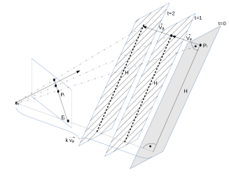
Figure 1: A 3D point $\vec{P}_{i}$ moves in three frames t=0,1,2 with a velocity vector $\vec{v}_{gi}$. The vector $\vec{v}_{gi}$ together with the corresponding point $\vec{P}_{i}$ defines a gray collision plane with $\vec{v}_{gi}$ as its normal vector.

It is obvious that relative motions of the camera $\vec{v}_{c}$ and the motion of a point on an object $\vec{v}_{i}$ in the environment are observed as an apparent combined motion vector $\vec{v}_{gi}=\vec{v}_{i}-\vec{v}_{c}$. The negative sign of $\vec{v_{c}}$ is due to the apparent additional motion of the object due to the motion of the camera. The sparse optical flow field reconstructed from point correspondences represents the projection of the resulting motion vector $\vec{v}_{gi}$, which can be treated as if only the point $p_{i}$ were moving in reference to a “static” camera.

Let us assume for now that a three-dimensional point $\vec{P}_{i}$ moves with an arbitrary constant velocity vector $\vec{v}_{gi}$ as depicted in Fig. 1. This motion results in a trace of projected points $p_{i}$ in consecutive image frames for time steps t={0,1,2}. The vector $\vec{v}_{gi}$ normal to the plane containing $P_{i}$ can be moved within this collision plane to align with the line going through the focal point of the camera. The corresponding intersection point $E_{i}$ of this line with the camera plane represents the projection of the observed point $P_{i}$ at infinite distance from the camera $-k\cdot\vec{v}_{gi}\rightarrow\infty$. Similar to the time-to-collision (TTC) approaches, the projected point $p_{i}$ moves from the epipole $E_{i}$ away along the line drawn in the camera image plane, while the 3D point $\vec{P}_{i}$ moves closer to the camera in the scene.

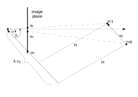
Figure 2: Projection in the plane of the set of projection triangles from Fig. 1.

For a safe navigation in a dynamic environment, it is often more important to understand the collision relations than the true metric distances to objects. So can a close object move in the same direction as the camera itself, while a distant object may be approaching the camera with a high speed. The measure for the relevance of a 3D point $P_{i}$ can be replaced by estimating the time-to-collision (TTC) as the length $k$ (Fig. 2), which tells the number of frames k (k is a float number) until the collision plane containing the point $P_{i}$ reaches the focal point of the camera. This value can be calculated directly from the image information without any additional extrinsic calibration data. We re-draw Fig. 1 in a way that the set of projection triangles lies in the image plane (Fig. 2). A projection point $p_{i}=(x_{i},y_{i},f)^{T}$ with f being the focal length in pixels can be converted into an angle relative to the optical axis (Fig. 2) first (1):

$$\gamma_{i}=\arctan\frac{u_{i}}{f},\quad\alpha=\gamma_{u_{a}}-\gamma_{u_{e_{i}}},\quad\beta=\gamma_{u_{b}}-\gamma_{u_{e_{i}}}$$ (1)

The value k is reduced by 1 with each new frame. Therefore, we can write the following equation (2):

$$\tan\alpha=\frac{H}{k\cdot||\vec{v}_{gi}||},\quad\tan\beta=\frac{H}{(k-1)\cdot||\vec{v}_{gi}||},\quad\tan\alpha\cdot k\cdot||\vec{v}_{gi}||=\tan\beta\cdot(k-1)\cdot||\vec{v}_{gi}||$$

$$\Rightarrow k=\frac{\tan\beta}{\tan\beta-\tan\alpha}$$ (2)

2.1 Simplified Motion Cases

Planar Motion

- The problem with equation (2) is the missing knowledge about the epipole position $E_{i}$ for a given observed motion of a point $p_{i}$. There are special cases for which the value k can be estimated directly from the motion of a single point in two images. We can tell directly from Fig. 2 that for all motions entirely in a horizontal plane, e.g. on the office floor or road, the epipole must lie on the horizon line in the image. This follows directly from the requirement that the motion vector $v_{gi}$ needs to be moved in the plane until it goes through the focal point, which is a point on the horizon. Since there is no vertical component of the velocity for this case, the epipole needs to be in the horizontal plane of the focal point. If the observed point has some height above the ground that moves it away from horizon line then the position of the epipole $e_{i}$ can be found as the intersection of the optical flow line with the horizon line. The intersection point becomes increasingly more accurate, the further the observed point is from the horizontal plane, which means the further the evaluated 3D point is from the ground or the closer the camera is to the observed object. The image position of $e_{i}=(u_{e},v_{e})^{T}$ defines the direction of the motion vector to be along the vector $v_{gi}=(u_{e},v_{e},f)^{T}$ with f being the focal length in pixels according to the definition in Fig. 1 and Fig. 3. We can estimate the distance value k with equation (2). As usual in structure from motion approaches, we cannot estimate the absolute motion value. The "depth" is composed from the number of frames k until the collision plane of the point $P_{i}$ reaches the focal point of the camera and the corresponding orthogonal value H (Fig. 2) to (3):

$$H=k\cdot\tan\alpha,\quad\vec{v}_{gi}=\frac{\vec{e}_{i}}{||\vec{e}_{i}||},\quad\vec{v}_{H}=\frac{(\vec{v}_{gi}\times\vec{p}_{i})\times\vec{v}_{gi}}{||(\vec{v}_{gi}\times\vec{p}_{i})\times\vec{v}_{gi}||}\quad\Rightarrow\quad\quad\vec{P}^{\prime}_{i}=k\cdot\vec{v}_{gi}+H\cdot\vec{v}_{H}$$ (3)

The expression $\vec{v}_{H}$ is a virtual shift within the collision plane that allows to find the displacement factor H that tells us, how far the point is from the direct collision with the focal point. All distance parameters are expressed in collision times TTC. It is interesting to see that for an in-plane motion in a static environment, the system can estimate the motion relative to any object from merely pixel data of one point on the object. In dynamic scenes, the notion of depth is replaced by the notion of how soon a collision plane including the point passes through the focal point of the camera. The values (k,H) describe when and in what distance from the focal point the “collision” will occur.

Direct Collision Candidate

- Another special case exists, when the observed point is directly in the epipole $e_{i}$ of the current motion. In this case, the distance H goes to zero (H=0). The point will always appear at the same position in the camera image. It becomes a static target. It is known in nautical applications as "constant bearing" often used to define collision candidates based on their apparent fixation at a specific angle (bearing) to the ship. The TTC expression for this point can only be calculated from the surrounding region around it.

Multiple Points on a Translating Object

- The epipole $e_{i}$ of an object can be understood as the point that will represent the object at very large distances from the camera. While the object approaches the camera with a given velocity $v_{gi}$, the points on the object expand from the epipole outwards. The direction of motion relative to the epipole can also be used to decide if the object approaches or escapes the camera. In the second case, the "collision" already happened. If the points of an object move away from the epipole then the collision is going to happen in k or it happened already k-frames ago in other case. We can find the position of the epipole in that case using the fact that all points on a rigid structure share the same epipole. The line segments defined by at least two points on the object will intersect exactly in the epipole $e_{i}$ (Fig. 3 left). Fig. 3 right shows that the direction of the relative motion between the camera and the object $\vec{T}$ can be obtained directly from the position of the epipole. $(F_{1},F_{2})$ are the corresponding focal points for the two camera images of the sequence if we consider the relative motion to be performed by the camera.

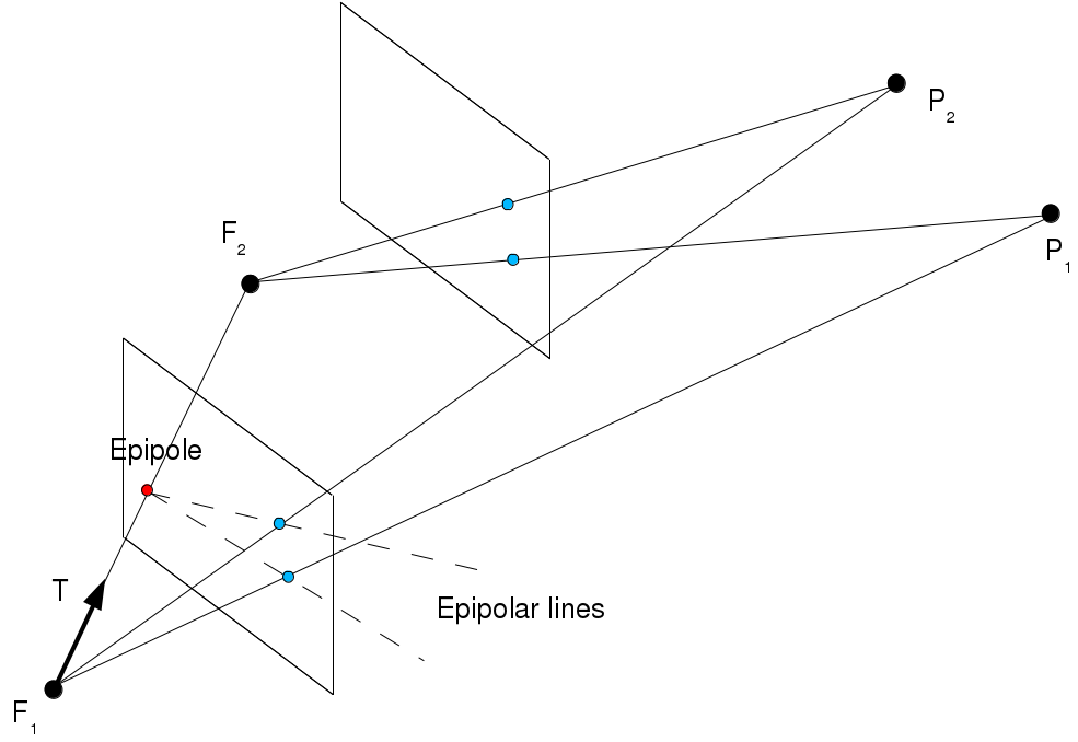
Figure 3: Epipole $e_{i}$ can be found from the intersection of the optical flow lines of at least two points on a rigid object, iff there is no rotation involved.

For a set of corresponding points between two images with $\{\vec{p}_{i}\}$ being 2D image points in the first image and $\{\vec{p^{\prime}}_{i}\}$ being corresponding image points in the second image, we can calculate the epipole $e_{x}$ to (4).

$$\begin{matrix}\vec{t}_{i}=\vec{p^{\prime}}_{i}-\vec{p}_{i}=(t_{ix},t_{iy})^{T},\quad\vec{n}_{i}=\frac{(-t_{iy},t_{ix})^{T}}{||(-t_{iy},t_{ix})^{T}||},\quad\tilde{A}=\left(\begin{matrix}\vec{n}_{1}^{T}\\ \vec{n}_{2}^{T}\\ \dots\end{matrix}\right),\quad\vec{b}=\left(\begin{matrix}\vec{p}_{1}^{T}\vec{n}_{1}\\ \vec{p}_{2}^{T}\vec{n}_{2}\\ \dots\end{matrix}\right),\\ \Rightarrow\quad\vec{e}_{x}=\tilde{A}^{-*}\cdot\vec{b}\end{matrix}$$ (4)

The optical flow vector $\vec{t}_{i}$ is calculated from point correspondences. Switching and negating entries of the vector result in a normal vector $\vec{n}_{i}$ orthogonal to the optical flow line from the current point correspondence. We stack all the possible matches from a rigid object in a matrix $\tilde{A}$. The pseudo-inverse calculation of $\tilde{A}^{-*}$ allows to calculate a least-square fit for the epipole $e_{x}$ to the current set of lines.

2.2 Clustering of Multiple Independent Motion Groups

For the case that we observe only translational motion of multiple objects including the camera, the motion clustering can be done based on the epipole estimation described in the previous paragraph. We use RANSAC to pick sets of point correspondences and calculate a hypothesis for the epipole using (4). Then we check all the normals to optical flow vectors $\vec{n}_{i}$ in (4) for the distance of the corresponding line to the epipole using (5):

$$\begin{matrix}\vec{l}_{i}=\vec{e}_{x}-\vec{p}_{i},\quad\Rightarrow\quad d_{i}=\left|\vec{n}_{i}^{T}\cdot\vec{l}_{i}\right|<\epsilon\end{matrix}$$ (5)

We calculate the projection of the connection vector $\vec{l}_{i}$ between the epipole $\vec{e}_{x}$ of the cluster and a point on the flow field $\vec{p}_{i}$. The calculated distance $d_{i}$ needs to be smaller than an epsilon distance to allow for detection errors in the camera image. We require also a similar TTC value for all the points of the cluster. All vectors that have a distance to the line smaller than an epsilon a grouped to one motion cluster and the remaining lines are ran through the RANSAC process iteratively again. We require that a cluster should have at least three line segments to be grouped together, because any two non-parallel lines intersect somewhere. Fig. 6 shows an example of clustering of objects based on their epipoles.

2.3 Finding Epipole for an Arbitrary Translational Motion

In case that the system observes a generic unconstrained motion in 3D space, the system needs to estimate the exact position of the epipole $e_{i}$ along the optical flow line that is constructed from point positions in consecutive images. In a generic case, the epipole $e_{i}$ in the image does not need to be on the horizon as it is the case for planar motion. In this case, an additional information from a third image is needed to estimate the position of the epipole from the change in the angular distances between the points (Fig. 4).

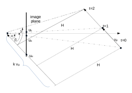
Figure 4: In a general motion case the epipole $e_{i}$ needs to be found from the position of a point tracked in three frames.

Our solution is to introduce an additional angular offset value x, which is added to the horizontal case with the angles $(\alpha,\beta)$ found from the intersection of with the horizontal line in the image as in the Planar Motion Case above. The true position is along the line away from the horizon shifted by an angle x. We can solve for this value by calculating the time to collision k in (2) for 2 consecutive frames of the sequence. The resulting difference between these values needs to be 1 since we reduced the number of frames by one. The solution for x is shown in (6):

$$\begin{matrix}\frac{\tan(\beta+x)}{\tan(\beta+x)-\tan(\alpha+x)}-\frac{\tan(\gamma+x)}{\tan(\gamma+x)-\tan(\beta+x))}\doteq 1,\quad\Rightarrow\quad x=\arctan\frac{\tan\alpha\cdot\tan\beta-2\tan\alpha\cdot\tan\gamma+\tan\beta\cdot\tan\gamma}{\tan\alpha-2\tan\beta+\tan\gamma}\end{matrix}$$ (6)

We used the MATLAB symbolic solver to find this solution for x. We see that all angular values $\{\alpha,\beta,\gamma\}$ representing the Planar Case have a constant correction value x that corrects for the true position of the epipole relative to the horizon line. We define $\{\alpha,\beta,\gamma\}$ in identical way as for the Planar Motion Case but need to add a correction value x that needs to be estimated from the evolution of the angular properties over three frames. This has a disadvantage that we need to assume that the motion between the frames remains constant over the period of three frames.

3 Experimental Results

We implemented the framework on a Linux system using AKAZE features from OpenCV to estimate the sparse optical flow in the images. We can estimate the correspondences between the images with 12Hz, which defines the time-base for our TTC calculations. A comparison with an existing benchmark database was not possible here, since databases like KITTY do not provide any motion data for the moving objects in the scene, which is done by this framework. An analysis of the sensitivity of the mathematical framework is provided here instead due to the lag of an appropriate ground-truth for comparisons.

3.1 Accuracy of the Parameter Estimation compared to a Bionocular Stereo Approach

Most systems estimate motion parameters (magnitude,direction) from consecutive reconstructions of the depth for a point $P_{i}(t)=(X_{i}(t),Y_{i}(t),Z_{i}(t))^{T}$ on an object for time-stamps t=0,1. While this provides a valid solution for indoor applications in service robotics, we need to consider that the depth in binocular stereo is estimated from the horizontal projection change between the two cameras $d(t)=x_{L}(t)-x_{R}(t)$ to:

$$d(t)=\frac{B\cdot f}{Z_{i}(t)}$$ (7)

with decreasing values of d(t) with increasing distance from the camera $Z_{i}(t)$. Given a constant detection accuracy for the matched features, the error become very soon in the range of the expected disparity value $d_{i}$ causing a large variation of the reconstructed point. The error gets propagated to the $(X_{i}(t),Y_{i}(t))$ values through the perspective projection equations.

For simplicity, let us compare the results with the planar case, where epipole position in the presented framework can be calculated directly from the intersection line of the flow segment with the horizon. The accuracy of direction depends on the accuracy of the intersection between the horizon and the line segment. The accuracy of the orientation of the segment increases with its length hence the detection accuracy can be assumed constant. We obtain following result for an object approaching with 50km/h with the motion direction of $45^{\circ}$, with a baseline of the stereo system of 15cm, focal length=8mm, and detection error $\Delta p=0.2$pixels.

We can see that the proposed framework gives still useful results even at high distance Z from the camera, where the reconstruction error from binocular stereo renders the data useless.

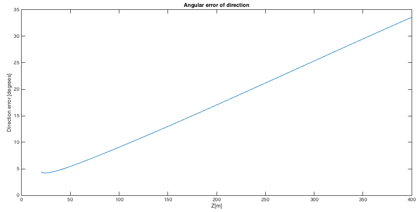
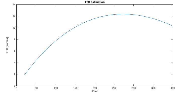
Figure 5: Orientation error and TTC estimates for the above example from the “collision planes” approach.

3.2 Planar Motion Examples

In case of a planar motion in the road scenario, we can drop the constraint on no rotation of the observed object that was required in Fig. 3. For the planar motion in the examples of this subsection, all motion vectors have only horizontal (x,z)-components and, therefore, lie on the horizon line. This horizon line in the image is estimated in a calibration process, where a resting camera observes multiple linear motions of objects with different relative directions. In the calibration process, at least two points on the moving object are selected to find the epipole. The horizon can be found by connecting the estimated epipoles for different directions (Fig. 6). A possible error in the epipole position is corrected before applying the calculations for the TTC from Eq. (2).

Fig. 6 shows an example with multiple independent motion components in the image. For clarity, just the ego-motion of the camera (yellow), the motion direction of the truck (red) and the motion direction of the bus in the circle (beige) are shown with their epipoles in the image. A zoomed version shows the different motion directions represented as the direction to the epipole of the corresponding vectors. We took just a few vectors for each of them to avoid too much clutter in the image. We see, that the bus in the roundabout has a different moving direction than the truck avoiding the road divider and the biker in front of the car.

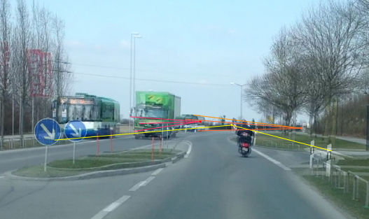
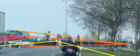
Figure 6: Dynamic scene with 3 exemplary motion components. The yellow epipole shows the direction of the eigen-motion of the camera, the beige epipole is the direction of motion for the bus in the circle, and the red epipole is the direction of motion for the truck (other deleted to reduce confusion).

3.3 Simulation Results

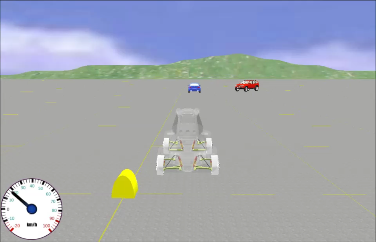
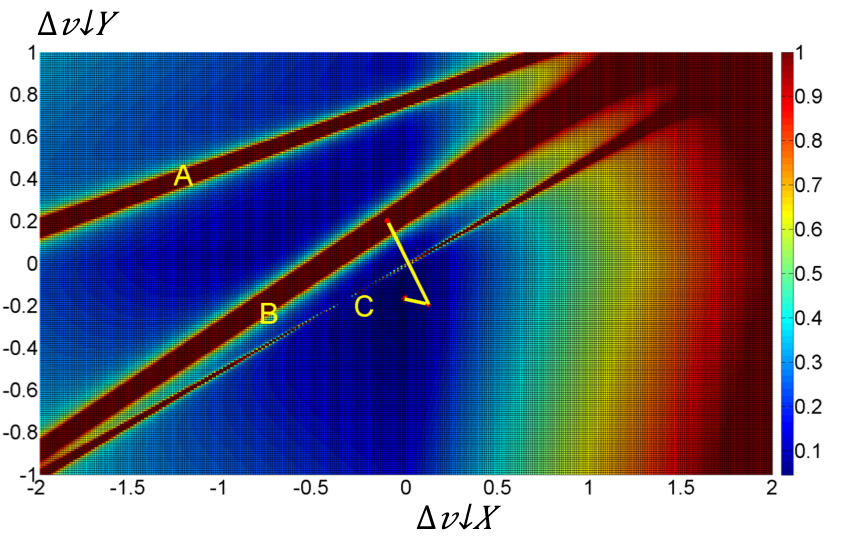
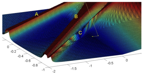
Figure 7: Collision map for a simulated scene on the top. The collision relations for different speed modifications of the own velocity in forwards and lateral directions are shown in the images below to be used for collision avoidance.

While the presented approach is used on our car for low-level collision avoidance, the correctness of the approach was validated on simulated scenes, where collisions can easily be defined and validated, The system is able to calculate collision relations for the dynamic scene with independently moving objects (Fig. 7). The system can calculate the collision relations for different forwards and lateral velocity changes to the current vehicle speed (center of the planning map in Fig. 7bottom with $\Delta v=0$) and it allows to plan an evasion trajectory to avoid collisions.

4 Conclusions and Future Work

We presented a framework that allows to model the motion relations between moving objects in a dynamic environment. We used the collision properties of the planes including the observed point with the relative motion vector as a normal and their distance expressed as the time until this plane sweeps through the focal point of the camera to describe the motion properties of the scene. This formulation does not require any extrinsic calibration of the camera and allows a robust detection of collision candidates in front of the camera. Since the direction of motion for the observed point is not calculated from position changes in the 3D reconstructions of the scene in large distances from the camera, the resulting information is more reliable that the motion estimation from 3D readings. The modeling with the time-to-collision instead of metric distance as a parameter allows a better prioritization of collision candidates for the collision avoidance. An object in 10m distance with the same motion direction as the camera does not create any danger to the camera while an object 75 meters away approaching the camera with high speed needs to be considered with a high priority. While a search for such object is difficult in Cartesian representations of the world, the distant object will have a very small time-to-collision(TTC) while the TTC for the close object moving with the same speed and direction as the camera will approach infinity in our representation. We use this framework in SenseAndAvoid applications for planes and as a safety system for collision avoidance in automotive applications.

References

- [1] G. Adiv. Determining three-dimensional motion and structure from optical flow generated by several moving objects. IEEE Trans. Pattern Anal. Mach. Intell., 7(4):384–401, 1985.
- [2] R. I. Hartley and A. Zisserman. Multiple View Geometry in Computer Vision. Cambridge University Press, ISBN: 0521540518, second edition, 2004.
- [3] M. Irani, P. Anandan, J. Bergen, R. Kumar, and S. Hsu. Efficient representations of video sequences and their applications. Signal Processing: Image Communication, 8(4):327–351, 1996.
- [4] M. Irani, P. Anandan, and M. Cohen. Vision Algorithms: Theory and Practice: International Workshop on Vision Algorithms Corfu, Greece, September 21–22, 1999 Proceedings, chapter Direct Recovery of Planar-Parallax from Multiple Frames, pages 85–99. Springer Berlin Heidelberg, Berlin, Heidelberg, 2000.
- [5] H. Li and R. Hartley. Five-point motion estimation made easy. In Proceedings of the 18th International Conference on Pattern Recognition - Volume 01, ICPR ’06, pages 630–633, Washington, DC, USA, 2006. IEEE Computer Society.
- [6] E. Mair, M. Suppa, and D. Burschka. Error Propagation in Monocular Navigation for Zinf Compared to Eightpoint Algorithm. In Proceedings of the IEEE/RSJ International Conference on Intelligent Robots and Systems (IROS’13), November 2013.
- [7] J. Revaud, P. Weinzaepfel, Z. Harchaoui, and C. Schmid. EpicFlow: Edge-preserving interpolation of correspondences for optical flow. In Conference on Computer Vision and Pattern Recognition, CVPR 2015, Boston, MA, USA, June 7-12, 2015, pages 1164–1172, 2015.
- [8] A. Roussos, C. Russell, R. Garg, and L. de Agapito. Dense multibody motion estimation and reconstruction from a handheld camera. In 11th IEEE International Symposium on Mixed and Augmented Reality, ISMAR 2012, Atlanta, GA, USA, November 5-8, 2012, pages 31–40, 2012.
- [9] A. Talukder and L. Matthies. Real-time detection of moving objects from moving vehicles using dense stereo and optical flow. In Intelligent Robots and Systems, 2004. (IROS 2004). Proceedings. 2004 IEEE/RSJ International Conference on, volume 4, pages 3718–3725, 2004.
- [10] W. B. Thompson and T.-C. Pong. Detecting moving objects. International Journal of Computer Vision, 4(1):39–57, 1990.
- [11] J. R. Tresilian. Perceptual information for the timing of interceptive action. Perception, 19(2):223–239, 1990.
- [12] B. Triggs. European Conference on Computer Vision Dublin, Ireland, 2000 Proceedings, Part I, chapter Plane + Parallax, Tensors and Factorization, pages 522–538. Springer Berlin Heidelberg, Berlin, Heidelberg, 2000.
- [13] L. Valgaerts, A. Bruhn, and J. Weickert. A Variational Model for the Joint Recovery of the Fundamental Matrix and the Optical Flow. In DAGM-Symposium, volume 5096 of Lecture Notes in Computer Science, pages 314–324. Springer, 2008.
- [14] R. Vidal, Y. Ma, and S. Sastry. Generalized principal component analysis (GPCA). Conference on Computer Vision and Pattern Recognition CVPR 2003, 16-22 June 2003, Madison, WI, USA, pages 621–628, 2003.
- [15] R. Vidal and A. Ravichandran. Optical flow estimation and segmentation of multiple moving dynamic textures. In Conference on Computer Vision and Pattern Recognition, 20-26 June 2005, San Diego, CA, USA, pages 516–521, 2005.
- [16] J. Weber and J. Malik. Rigid Body Segmentation and Shape Description from Dense Optical Flow Under Weak Perspective. IEEE Trans. Pattern Anal. Mach. Intell., 19(2):139–143, 1997.
- [17] A. Wedel, D. Cremers, T. Pock, and H. Bischof. Structure- and motion-adaptive regularization for high accuracy optic flow. In International Conference on Computer Vision, ICCV 2009, Kyoto, Japan, September 27 - October 4, 2009, pages 1663–1668, 2009.
- [18] K. Yamaguchi, D. McAllester, and R. Urtasun. Robust monocular epipolar flow estimation. In Computer Vision and Pattern Recognition (CVPR), 2013 IEEE Conference on, pages 1862–1869, 2013.