Quasi-phases and pseudo-transitions in one-dimensional models with nearest neighbor interactions

Abstract

There are some particular one-dimensional models, such as the Ising-Heisenberg spin models with a variety of chain structures, which exhibit unexpected behaviors quite similar to the first and second order phase transition, which could be confused naively with an authentic phase transition. Through the analysis of the first derivative of free energy, such as entropy, magnetization, and internal energy, a "sudden" jump that closely resembles a first-order phase transition at finite temperature occurs. However, by analyzing the second derivative of free energy, such as specific heat and magnetic susceptibility at finite temperature, it behaves quite similarly to a second-order phase transition exhibiting an astonishingly sharp and fine peak. The correlation length also confirms the evidence of this pseudo-transition temperature, where a sharp peak occurs at the pseudo-critical temperature. We also present the necessary conditions for the emergence of these quasi-phases and pseudo-transitions.

The absence of phase transitions in one-dimensional models with short range coupling was established since the 1950s, as discussed by van HoveHove . More recently, Cuesta and Sanchezcuesta investigated relevant properties regarding one-dimensional models, such as the general non-existence theorem at the finite temperature phase transition with short range interactiondyson-2 . Although there are some one-dimensional models with long-range interactions that exhibit phase transition at finite temperaturedyson-1 . Besides, some peculiar one-dimensional models exhibit at the finite temperature a first-order phase transition, such as the Kittel model (zipper model)kittel , Chui-Weeks modelchui and Dauxois-Peyrard modeldauxois .

Several real magnetic materials, such as $\mathrm{Cu_{3}(CO_{3})_{2}(OH)_{2}}$ known as natural mineral azurite kikuchi05 , were investigated using several approximate methods assuming the Heisenberg model to describe the natural mineral azuriteLau . In addition, Honecker et alhonecker investigated the thermodynamic properties of the Heisenberg model in a diamond chain structure. Furthermore, in the last decade, the thermodynamics of the Ising-Heisenberg model in diamond chains has also been widely discussed in referencesvalverde ; Cano ; orojas ; Lisnii-1 .

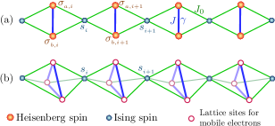
Figure 1: Schematic representation: (a) Ising-XYZ diamond chain modeltorrico2 . (b) Double-tetrahedral chain, with localized Ising spin regularly alternates with two mobile electrons delocalized over a triangular plaquetteGalisova .

Lately, several one-dimensional models have been investigated in the framework of decorated structures, particularly Ising and Heisenberg models with a variety of structures, such as the Ising-Heisenberg models in diamond chain structuretorrico ; torrico2 as shown in fig.1a, one-dimensional double-tetrahedral chain (see fig.1b), in which the localized Ising spin regularly alternates with two mobile electrons delocalized over a triangular plaquetteGalisova , alternating Ising-Heisenberg ladder modelon-strk , Ising-Heisenberg triangular tube modelstrk-cav . The analysis of the first derivative of the thermodynamic potential, such as entropy, internal energy, magnetization shows a significant jump as a function of temperature, maintaining a close similarity with the first order phase transition. Similarly, a second order derivative of potential thermodynamics, such as specific heat and magnetic susceptibility, resembles a typical second order phase transition at finite temperature.

Quasi-phases and pseudo-transitions:

Most one-dimensional models with short-range interaction have been extensively investigated in the last decadevalverde ; Cano ; orojas ; Lisnii-1 ; torrico ; torrico2 ; Galisova , whose transfer matrix have the following structure $\mathbf{T}=\left[\begin{array}[]{cc}w_{0}&w_{1}\\ w_{1}&w_{2}\end{array}\right]$. Obviously, the corresponding eigenvalues are given by $\lambda_{\pm}=\tfrac{1}{2}\Bigl{(}w_{0}+w_{2}\pm\sqrt{(w_{0}-w_{2})^{2}+4w_{1}^{2}}\Bigr{)}$, where $w_{n}=\sum_{k=0}{\rm e}^{-\beta\varepsilon_{n,k}}$ are the Boltzmann factors, with $\varepsilon_{n,k}$ being the energy levels $k=\{0,1,\ldots\}$ for each sector $n=0$, 1 and 2. For simplicity, here we are considering only the non-degenerate case since its extension to the degenerate case is trivial. Where $\beta=1/k_{B}T$ with $k_{B}$ Boltzmann constant and $T$ the absolute temperature.

Therefore, for a periodic chain with $N$ unit cell, the partition function can be expressed by $\mathcal{Z}_{N}=\lambda_{+}^{N}+\lambda_{-}^{N}$, while the free energy per unit cell in thermodynamic limit becomes

$$f=-\frac{1}{\beta}\ln\left[\tfrac{1}{2}\Bigl{(}w_{0}+w_{2}+\sqrt{(w_{0}-w_{2})^{2}+4w_{1}^{2}}\Bigr{)}\right].$$ (1)

Now let us ask the following question, what happens to the free energy $f$ when $w_{1}=0$? This means that free energy can be described as $f=-\frac{1}{\beta}\ln(w_{0})$ for $w_{0}>w_{2}$, whereas $f=-\frac{1}{\beta}\ln(w_{2})$ for $w_{0}<w_{2}$, or simply expressed by $f=\min\bigl{\{}-\frac{1}{\beta}\ln(w_{0}),-\frac{1}{\beta}\ln(w_{2})\bigr{\}}$, which is piecewise function. On the other hand, the transfer matrix $\mathbf{T}$ becomes diagonal matrix with elements $w_{0}$ and $w_{2}$. The limit $w_{0}=w_{2}$ leads to a transcendental equation involving the temperature, and this one can be solved numerically, from which we can find a genuine critical temperature.

In particular the Hamiltonian for the one-dimensional Ising model with spin-1/2 is $\mathcal{H}=\sum_{i}(-Js_{i}s_{i+1}-hs_{i})$. The energies per unit cell are $\varepsilon_{0,0}=-\frac{J}{4}-\frac{h}{2}$ for ($s_{i},s_{i+1}$) $\rightarrow$ ($\uparrow,\uparrow$), $\varepsilon_{2,0}=-\frac{J}{4}+\frac{h}{2}$ for ($s_{i},s_{i+1}$) $\rightarrow$ ($\downarrow,\downarrow$), and $\varepsilon_{1,0}=\frac{J}{4}$ for ($s_{i},s_{i+1}$) $\rightarrow$ ($\uparrow,\downarrow$) or ($\downarrow,\uparrow$), thus the Boltzmann factors simply reduce to: $w_{0}={\rm e}^{-\beta\varepsilon_{0,0}}$, $w_{1}={\rm e}^{-\beta\varepsilon_{1,0}}$ and $w_{2}={\rm e}^{-\beta\varepsilon_{2,0}}$. Despite the above condition $w_{1}\rightarrow 0$ occurs when $J\rightarrow\infty$, we will never have the competing condition between $w_{0}$ and $w_{2}$ for $h>0$. Besides, the condition $w_{0}=w_{2}$ for the Ising one-dimensional Ising model just implies $\varepsilon_{0,0}=\varepsilon_{2,0}$ and obviously there is no non-zero "critical temperature".

But is it possible that $w_{1}=0$? Note that $w_{1}=\sum_{r=0}{\rm e}^{-\beta\varepsilon_{1,r}}$. So we conclude that we will never have $w_{1}=0$, for $\beta<\infty$. Thus from now on, we will rigorously analyze the case $w_{1}>0$.

Several "decorated" one-dimensional modelsvalverde ; Cano ; orojas ; Lisnii-1 (and references there in) satisfy the following condition $w_{0}\sim w_{2}\sim w_{1}$ and $|w_{0}-w_{2}|\sim 2w_{1}$, with well-known thermodynamic properties. However, there are some particular modelstorrico2 ; Galisova ; on-strk ; strk-cav that satisfy the following condition $w_{0}\sim w_{2}\ggg w_{1}$ and $|w_{0}-w_{2}|\gg 2w_{1}$. The free energy using the Taylor series expansion around $w_{1}\rightarrow 0$, results in

$$f\approx\begin{cases}-\tfrac{1}{\beta}\ln(w_{0})-\tfrac{1}{\beta}\tfrac{w_{1}^{2}}{w_{0}^{2}},&w_{0}\geqslant w_{2}\\ -\tfrac{1}{\beta}\ln(w_{2})-\tfrac{1}{\beta}\tfrac{w_{1}^{2}}{w_{2}^{2}},&w_{0}<w_{2}\end{cases}.$$ (2)

To analyze the most relevant behavior of (1) without losing its generality, we consider only a couple of lowest energies for each Boltzmann factors (as described in the figure 2a), using this feature each sector can be expressed as: For ($n=0$), the Boltzmann factor reduce to $w_{0}={\rm e}^{-\beta\varepsilon_{0,0}}+{\rm e}^{-\beta\varepsilon_{0,1}}$ with $\varepsilon_{0,0}<\varepsilon_{0,1}$. For ($n=1$) the $w_{1}={\rm e}^{-\beta\varepsilon_{1,0}}+{\rm e}^{-\beta\varepsilon_{1,1}}$ depends of the low-lying excited energies $\varepsilon_{1,0}$ and $\varepsilon_{1,1}$. Whereas, for ($n=2$) the $w_{2}={\rm e}^{-\beta\varepsilon_{2,0}}+{\rm e}^{-\beta\varepsilon_{2,1}}$ are given in terms of $\varepsilon_{2,0}$ and $\varepsilon_{2,1}$.

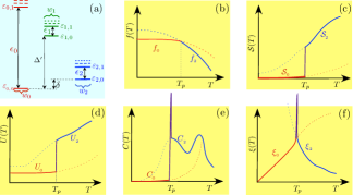
Figure 2: (a) Low-lying energy levels. (b) Free energy, (c) Entropy, (d) Internal energy, (e) Specific heat, and (f) correlation length as a function of temperature. With $T_{p}$ being the pseudo critical temperature.

The energy gaps outlined in fig.2a are $\epsilon_{0}=\varepsilon_{0,1}-\varepsilon_{0,0}$, $\epsilon_{1}=\varepsilon_{1,1}-\varepsilon_{1,0}$, $\epsilon_{2}=\varepsilon_{2,1}-\varepsilon_{2,0}$, $\Delta^{\prime}=\varepsilon_{1,0}-\varepsilon_{0,0}$ and $\delta=\varepsilon_{2,0}-\varepsilon_{0,0}$. The above condition of $w_{n}$’s in terms of energy gaps become roughly $\delta\sim\epsilon_{2}\ll 2\Delta^{\prime}\lesssim\epsilon_{0}$, and define conveniently $\Delta={\rm min}(\Delta^{\prime},\epsilon_{0}/2)$.

In fig.2b is illustrated the free energy $f_{0}\approx\varepsilon_{0,0}-T\,{\rm e}^{-\frac{2\Delta}{T}}$ when $w_{0}>w_{2}$, which is weakly dependent of other energy levels, because the main contribution of the free energy is $\varepsilon_{0,0}$. While for $w_{0}<w_{2}$, the free energy $f_{2}\approx\varepsilon_{2,0}-T\,\ln\left(1+{\rm e}^{-\epsilon_{2}/T}\right)$ depends more significantly of $\epsilon_{2}$. Although free energy resembles a piecewise function, exact free energy(1) is an analytic function or an infinitely differentiable function.

When $w_{1}\ll 1$, the transfer matrix $\mathbf{T}$ is a quasi diagonal matrix, with competing $w_{0}$ and $w_{2}$, so the condition $w_{0}=w_{2}$ lead us to a transcendental equation in temperature or any other Hamiltonian parameter, so this equation can be solved numerically to find a "pseudo-critical" temperature $T_{p}$.

In fig.2c is depicted schematically the entropy $\mathcal{S}(T)$ as a function of the temperature, for $w_{0}>w_{2}$ or $T<T_{p}$ we observe the entropy would be almost a constant curve $\mathcal{S}_{0}\approx\left(1+\frac{2\Delta}{T}\right){\rm e}^{-2\Delta/T}$, whereas the entropy "suddenly" increases at $T_{p}$ and for $w_{0}\leqslant w_{2}$ or $T_{p}\leqslant T$ it increases significantly as soon the temperature increases with $\mathcal{S}_{2}\approx\ln(1+{\rm e}^{-\epsilon_{2}/T})+\frac{\epsilon_{2}}{T}\left(1+{\rm e}^{\epsilon_{2}/T}\right)^{-1}$. Indeed, some evidence of this behavior has already been observed in previous workGalisova ; on-strk ; strk-cav ; timonin , and spin-ice model with short-range interaction in the Bethe-Peierls approachtimonin . The entropy behavior reveals the similarity with the first-order phase transitionSauera , so it is interesting to define the "latent heat" associated with the system in $T_{p}$ as $\mathcal{L}\propto Q\equiv T_{p}\left(\mathcal{S}_{2}(T_{p})-\mathcal{S}_{0}(T_{p})\right)=T_{p}\varDelta\mathcal{S}_{2,0}$.

The internal energy $U(T)$ is also depicted schematically in fig.2d, where we can observe a nearly constant energy $U_{0}\approx\varepsilon_{0,0}+2\Delta{\rm e}^{-2\Delta/T}$ for $T<T_{p}$, whereas for $T_{p}<T$ the thermal excitation significantly influences the internal energy $U_{2}\approx\varepsilon_{2,0}+\epsilon_{2}\left(1+{\rm e}^{\epsilon_{2}/T}\right)^{-1}$ like in most one-dimensional models. Again the jump in internal energy shows the similarity to the first order phase transitionSauera , so alternatively we can express the "latent heat" as $\mathcal{L}=Q=U_{2}(T_{p})-U_{0}(T_{p})=\delta+\epsilon_{2}(1+{\rm e}^{\epsilon_{2}/T_{p}})^{-1}-2\Delta{\rm e}^{-2\Delta/T_{p}}$, this quantity reinforces the first-order pseudo-transition.

However, since the free energy is an analytic function, the second derivative of the free energy near the pseudo-transition temperature exhibits an impressively fine peak quite similar to a cusp-like singularity of second-order phase transition, as occurs in magnetic susceptibility and specific heat (see fig.2e). Near the pseudo-critical temperature, the specific heat becomes $C_{0}\approx\left(\tfrac{2\Delta}{T}\right)^{2}{\rm e}^{-2\Delta/T}$ for $T<T_{p}$ and $C_{2}\approx\left(\tfrac{\epsilon_{2}}{T}\right)^{2}{\rm e}^{-\epsilon_{2}/T}\left(1+{\rm e}^{-\epsilon_{2}/T}\right)^{-2}$ for $T_{p}<T$. Some evidence of this effect has already been observed in one-dimensional models such as those discussed in the literatureGalisova ; on-strk ; strk-cav .

It is also worth investigating the correlation length $\xi$ illustrated in fig.2f (i.e. nodal Ising spin correlation length), which is given by $\xi^{-1}=\ln\left(\tfrac{\lambda_{+}}{\lambda_{-}}\right)$. Using the Taylor series expansion analogous to eq.(2) when $w_{1}\rightarrow 0$, the correlation length becomes,

$$\xi^{-1}\approx \begin{cases}\ln\left(\tfrac{w_{0}}{w_{2}}+\tfrac{w_{1}^{2}}{w_{2}^{2}}\right),&w_{0}>w_{2}\\ \ln\left(\tfrac{w_{2}}{w_{0}}+\tfrac{w_{1}^{2}}{w_{0}^{2}}\right),&w_{0}<w_{2}\end{cases}.$$ (3)

The leading terms of the correlation length can be expressed by $\xi_{0}\approx\left\{\frac{\delta}{T}-\ln\left(1+{\rm e}^{-\epsilon_{2}/T}\right)\right\}^{-1}$ for $T<T_{p}$, and $\xi_{2}\approx\left\{-\frac{\delta}{T}+\ln\left(1+{\rm e}^{-\epsilon_{2}/T}\right)\right\}^{-1}$ for $T_{p}<T$. Of course, this expression is valid around the pseudo-critical temperature, and this expression give us simply a maximum in $T=T_{p}$, and not a cusp-like singularity.

The present analysis could be applied to any physical system that has the form of free energy (1). Here, we only discuss how the unusual properties arise near the pseudo-critical temperature $T_{p}$.

Now let us consider as an illustrative example the one-dimensional Ising-XYZ model in the diamond chain structure which was solved exactly in the referencestorrico ; torrico2 .

Ising-XYZ diamond chain:

In fig.1a, the Ising-XYZ diamond chain structure is schematically illustrated. Where $s_{i}$ represents the Ising spin-1/2, and $\sigma_{a(b),i}^{\alpha}$ denotes the Heisenberg spin-1/2, assuming $\alpha=\{x,y,z\}$, whose Hamiltonian and its exact solution was given in reference torrico2 .

The couples of low-lying energy levels for each sector $w_{n}$ are:

(i) For sector $n=2$ ($\uparrow\uparrow$ ) the first low-lying energy is

$$\varepsilon_{2,0}=E_{{}_{MF_{2}}}=-\tfrac{J_{z}}{4}-\tfrac{h}{2}-\sqrt{(h+J_{0})^{2}+\tfrac{1}{4}J^{2}\gamma^{2}},$$ (4)

(ferromagnetic Ising spin and modulated ferromagnetic Heisenberg spin ($MF_{2}$) phase), and the other energy level is

$$\varepsilon_{2,1}=E_{{}_{FI}}=-\tfrac{J+h}{2}+\tfrac{J_{z}}{4},$$ (5)

(ferrimagnetic (FI) phase).

The corresponding ground states are expressed by

$$|MF_{n}\rangle= \overset{N}{\underset{i=1}{\prod}}c_{n}\left(\alpha_{n}|\begin{smallmatrix}+\\ +\end{smallmatrix}\rangle_{i}+|\begin{smallmatrix}-\\ -\end{smallmatrix}\rangle_{i}\right)\otimes|\tau\rangle_{i},$$ (6)

$$|FI\rangle= \overset{N}{\underset{i=1}{\prod}}\tfrac{1}{\sqrt{2}}\left(|\begin{smallmatrix}-\\ +\end{smallmatrix}\rangle_{i}+|\begin{smallmatrix}+\\ -\end{smallmatrix}\rangle_{i}\right)\otimes|+\rangle_{i},$$ (7)

where $\alpha_{n}=\frac{-J\gamma}{2h+2J_{0}\mu-2A_{n}}$, $c_{n}=\frac{1}{\sqrt{1+\alpha_{n}^{2}}}$ and $A_{n}=\sqrt{\left(h+J_{0}(n-1)\right)^{2}+\tfrac{1}{4}J^{2}\gamma^{2}}$. The state $MF_{2}$ is obtained fixing $n=2$ and $\tau=+$.

(ii) Whereas in sector $n=0$ ($\downarrow\downarrow$), we have the ground state energy, whose energy becomes

$$\varepsilon_{0,0}=E_{{}_{MF_{0}}}=-\tfrac{J_{z}}{4}+\tfrac{h}{2}-\sqrt{(h-J_{0})^{2}+\tfrac{1}{4}J^{2}\gamma^{2}}.$$ (8)

The corresponding modulated ferromagnetic ($MF_{0}$) state is given by (6) when $n=0$ and $\tau=-$. Whereas, the first excited energy in this sector is $\varepsilon_{0,1}=\frac{J_{z}}{4}-\frac{J-h}{2}$.

(iii) Analogously, for sector $n=1$ ($\downarrow\uparrow$ or $\uparrow\downarrow$) a couple of low-lying excited energy levels are $\varepsilon_{1,0}=\frac{J_{z}}{4}-\frac{J}{2}$ and $\varepsilon_{1,1}=-\frac{J_{z}}{4}-\frac{1}{2}\sqrt{4h^{2}+J^{2}\gamma^{2}}$.

"Quasi-phase" diagram for Ising-XYZ diamond chain:

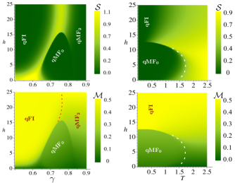
Figure 3: Density plot: Quasi-phase diagram for Ising-XYZ diamond chain at finite temperature, for fixed $J=100$, $J_{0}=-24$ and $J_{z}=24$. (Left) for fixed $T=1$, (right) for fixed $\gamma=0.7$.

All plots below were performed using the exact result torrico2 , while the low temperature limit discussed above fits nicely with the exact result.

In fig.3(left-top) the density plot for the entropy in the $\gamma-h$ plane is shown for the parameters given in the legend of fig.3, this plot resembles the vestiges of the phase diagram at zero temperaturetorrico2 . Then due to the thermal excitation, these phases will be called as "quasi-phase", the boundary between $qFI$-$qMF_{2}$ ($FI$-$MF_{2}$ at $T=0$) there is a standard phase transition signaling that becomes smooth due to thermal excitation. However, the boundary between $qFI$-$qMF_{0}$ ($FI$-$MF_{0}$ ) and $qMF_{0}$ -$qMF_{2}$ ($MF_{0}$ -$MF_{2}$ ) exhibits an uncommonly well-defined boundary around the $qMF_{0}$ region, and this region seems insensitive to thermal excitation, this is because in this region there is a large energy gap $2\Delta$. This phenomenon is very unusual for one-dimensional models, because any traces of zero temperature must be fade away as the temperature increases. A similar plot is depicted for the magnetization in fig.3(left-bottom), the density plot illustrates the magnetization for the same set of entropy parameters. We can observe the boundary between $qFI$-$qMF_{2}$ is almost imperceptible, here is marked by dashed line just to follow the phase transition pattern. However, the boundary between $qFI$-$qMF_{0}$ and $qMF_{0}$ -$qMF_{2}$ is completely different with clearly sharp boundary, rounding the $qMF_{0}$ region.

Now let us show in fig.3(right) the quasi-phase diagram in the $h$-$T$ plane, the density plot for entropy (top) and magnetization (bottom). For most one-dimensional models, this type of diagram will only show traces of phase transition at zero temperature which readily disappears when the temperature increases. However, here the entropy/magnetization density plot illustrates that the sharp boundary clearly survives at finite temperature, and seems almost independent of thermal excitation, although at a higher temperature that sharp boundary vanishes.

In fig.4 is illustrated the pseudo-transition temperature for the Ising-XYZ diamond chaintorrico2 , where an extremely strong fine peak occurs for specific heat (a), magnetic susceptibility (b) and correlation length between nodal Ising spins(c). All panels are conveniently drawn on logarithmic scales. It is worth mentioning that this peak never goes to infinity, the smaller the $T_{p}$ the thinner and stronger the peak becomes. Note that in panel (a) and (b) the red dashed line apparently shows the absence of peaks, but there is an astonishingly thin and vigorous peak. Indeed, only for $T_{p}=0$ the peak leads to infinity indicating a genuine phase transition, which is in agreement with the phase transition theoremcuesta .

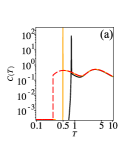
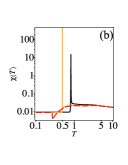
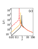
Figure 4: Ising-XYZ diamond chaintorrico ; torrico2 : (a) Specific heat as a function of temperature temperature. (b) Magnetic susceptibility. In (c) correlation length $\xi(T)$ as a function of temperature. Assuming fixed parameters $J=100$, $J_{0}=-24$ and $J_{z}=24$ and $\gamma=0.7$ for $h=12$ (black line), $h=12.6$ (orange line) and $h=12.74$ (red dashed line).

Conclusions.

Although, there are no real phase transitions in the one-dimensional model. For some special cases of Ising-Heisenberg one-dimensional spin models, the analysis of internal energy, entropy and magnetization show a pseudo-transition quite similar to a first-order phase transition, where we associate a "latent heat" to reinforce this propertySauera . While for specific heat and magnetic susceptibility it exhibits an extremely sharp peak indicating a "pseudo-transition" between the quasi-phases, this pseudo-transition closely resembles a typical second-order phase transition. Some evidence of quasi-phase and pseudo-transitions have already been manifested in recent previous works, such as Ising-XYZ diamond chaintorrico2 , tetrahedral chainGalisova , Ising-Heisenberg ladder modelon-strk , Ising-Heisenberg triangular tube modelsstrk-cav . However, here we present a general condition for appearing this quasi-phases and pseudo-transitions. It is worth mentioning that this unexpected property is intrinsically related to the "decorated" lattice models. Evidently, this opens several possibilities of finding other "decorated" model with this property. Another relevant issue to note is that this result opens the possibility of researching and synthesizing real materials with this stunning property.

This work was partially supported by Brazilian agencies CNPq and FAPEMIG.

References

- (1) L. van Hove, Physica 16,137 (1950).
- (2) J. A. Cuesta and A. Sanchez, J. Stat. Phys. 115, 869 (2003).
- (3) F. J. Dyson, Comm. Math. Phys. 12, 212 (1969).
- (4) F. J. Dyson, Comm. Math. Phys. 12, 91 (1969).
- (5) C. Kittel, Am. J. Phys. 37, 917(1969).
- (6) S. T. Chui and John D. Weeks, Phys. Rev. B 23, 2438 (1981)
- (7) T. Dauxois and M. Peyrard, Phys. Rev. E 51, 4027 (1995).
- (8) H. Kikuchi, Y. Fujii, M. Chiba, S. Mitsudo, T. Idehara, T. Tonegawa, K. Okamoto, T. Sakai, T. Kuwai, and H. Ohta, Phys. Rev. Lett. 94, 227201 (2005).
- (9) A. Honecker and A. Lauchli. Phys. Rev. B 63, 174407 (2001); H. Jeschke et al., Phys. Rev. Lett. 106, 217201 (2011); N. Ananikian, H. Lazaryan, and M. Nalbandyan, Eur. Phys. J. B 85, 223 (2012).
- (10) A. Honecker, S. Hu, R. Peters J. Ritcher, J. Phys.: Condens. Matter 23, 164211 (2011).
- (11) J.S. Valverde, O. Rojas, S.M. de Souza, J. Phys. Condens. Matter 20, 345208 (2008); O. Rojas, S.M. de Souza, Phys. Lett. A 375, 1295 (2011).
- (12) L. Canova, J. Strecka, and M. Jascur, J. Phys: Condens. Matter 18, 4967 (2006).
- (13) O. Rojas, S. M. de Souza, V. Ohanyan, M. Khurshudyan, Phys. Rev. B 83 , 094430 (2011).
- (14) B. M. Lisnii, Low Temp. Phys. 37, 296 (2011); Ukrainian Journal of Physics 56, 1237 (2011).
- (15) J. Torrico, M. Rojas, S. M. de Souza, O. Rojas and N. S. Ananikyan, Eur. Phys. Lett. 108, 50007 (2014).
- (16) J. Torrico, M. Rojas, S. M. de Souza and O. Rojas, Phys. Lett. A 380, 3655 (2016).
- (17) L. Galisova and J. Strecka, Phys. Rev. E 91, 0222134 (2015)
- (18) O. Rojas, J. Strečka and S.M. de Souza, Sol. Stat. Comm. 246, 68 (2016).
- (19) J. Strecka, R. C. Alecio, M. Lyra and O. Rojas, J. Magn. Magn. Matter 409, 124 (2016).
- (20) P. N. Timonin, J. Exp. Theor. Phys. 113, 251 (2011).
- (21) T. Sauera, Eur. Phys. J. Special Topics 226, 539 (2017)