WRS: Waiting Room Sampling for Accurate Triangle Counting in Real Graph Streams

Abstract

If we cannot store all edges in a graph stream, which edges should we store to estimate the triangle count accurately?

Counting triangles (i.e., cycles of length three) is a fundamental graph problem with many applications in social network analysis, web mining, anomaly detection, etc. Recently, much effort has been made to accurately estimate global and local triangle counts in streaming settings with limited space. Although existing methods use sampling techniques without considering temporal dependencies in edges, we observe temporal locality in real dynamic graphs. That is, future edges are more likely to form triangles with recent edges than with older edges.

In this work, we propose a single-pass streaming algorithm called Waiting-Room Sampling (WRS) for global and local triangle counting. WRS exploits the temporal locality by always storing the most recent edges, which future edges are more likely to form triangles with, in the waiting room, while it uses reservoir sampling for the remaining edges. Our theoretical and empirical analyses show that WRS is: (a) Fast and ‘any time’: runs in linear time, always maintaining and updating estimates while new edges arrive, (b) Effective: yields up to 47% smaller estimation error than its best competitors, and (c) Theoretically sound: gives unbiased estimates with small variances under the temporal locality.

I Introduction

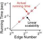
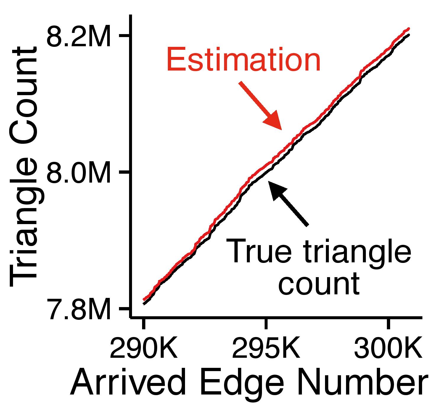
(a) WRS is fast and ‘any time’

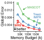
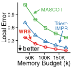
(b) WRS is effective

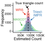
(c) WRS is unbiased

Figure 1: Strengths of WRS. (a) WRS scales linearly with the number of edges, and it always maintains the estimates of the triangle counts while input graphs grow with new edges. (b) WRS is more accurate than state-of-the-art streaming algorithms in global and local triangle counting. (c) WRS gives unbiased estimates (Theorem 1) with small variances (Lemma 2). The ArXiv dataset, explained in the experiment section, is used for all these figures.

In a dynamic graph stream, where new edges are streamed as they are created, how can we count the triangles? If we cannot store all the edges in memory, which edges should we store to estimate the triangle count accurately?

Counting the triangles (i.e., cycles of length $3$) in a graph is a fundamental problem with many applications. For example, triangles in social networks have received much attention as an evidence of homophily (i.e., people choose friends similar to themselves) [1] and transitivity (i.e., people with common friends become friends) [2]. Thus, many concepts in social network analysis, such as social balance [2], the clustering coefficient [3], and the transitivity ratio [4], are based on the count of triangles. Moreover, the count of triangles has been used for spam detection [5], web-structure analysis [6], degeneracy estimation [7], and query optimization [8].

Due to the importance of triangle counting, numerous algorithms have been developed in many different settings, including multi-core [9, 10], external-memory [10, 11], distributed-memory [12], and MapReduce [13, 14, 15] settings. The algorithms aim to accurately and rapidly count global triangles (i.e., all triangles in a graph) and/or local triangles (i.e., triangles that each node is involved with).

Especially, as many real graphs, including social media and web, evolve over time, recent work has focused largely on streaming settings where graphs are given as streams of new edges. To accurately estimate the count of the triangles in large graph streams not fitting in memory, various sampling techniques have been developed [16, 17, 18].

However, existing streaming algorithms sample edges without considering temporal dependencies in edges and thus cannot exploit temporal locality, i.e., the tendency that future edges are more likely to form triangles with recent edges than with older edges. This temporal locality is observed commonly in many real dynamic graph streams, where new edges are streamed as they are created.

Then, how can we exploit the temporal locality for accurately estimating global and local triangle counts? We propose Waiting-Room Sampling (WRS), a single-pass streaming algorithm that always stores the most recent edges in the waiting room, while it uses standard reservoir sampling [19] for the remaining edges. The waiting room increases the probability that, when a new edge arrives, edges forming triangles with the new edge are in memory. Reservoir sampling, on the other hand, enables WRS to yield unbiased estimates.

Specifically, our theoretical and empirical analyses show that WRS has the following strengths:

Fast and ‘any time’: WRS runs in linear time in the number of edges, giving the estimates of triangle counts at any time, not only at the end of streams (Figure 1(a)).

Effective: WRS produces up to 47% smaller estimation error than its best competitors (Figure 1(b)).

Theoretically sound: we prove the unbiasedness of the estimators provided by WRS and their small variances under the temporal locality (Theorem 1 and Figure 1(c)). Reproducibility: The code and datasets used in the paper are available at http://www.cs.cmu.edu/~kijungs/codes/wrs/.

In Section II, we review related work. In Section III, we introduce notations and the problem definition. In Section IV, we discuss temporal locality in real graph streams. In Section V, we propose our algorithm WRS. After showing experimental results in Section VI, we draw conclusions in Section VII.

II Related Work

In this section, we discuss previous work on global and local triangle counting in a graph stream with limited space.

Global triangle counting in graph streams: For estimating the count of global triangles (i.e., all triangles in a graph), Tsourakakis et al. [20] proposed sampling each edge i.i.d. with probability $p$. Then, the global triangle count can be estimated simply by multiplying that in the sampled graph by $p^{-3}$. Jha et al. [21] and Pavan et al. [22] proposed sampling wedges (i.e., paths of length $2$) instead of edges for better space efficiency. Kutzkov and Pagh [23] combined edge and wedge sampling methods for global triangle counting in graph streams where edges can be both inserted or deleted.

Local triangle counting in graph streams: For estimating the count of local triangles (i.e., triangles with each node), Lim and Kang [17] proposed sampling each edge i.i.d with probability $p$ but updating global and local counts whenever an edge arrives, even when the edge is not sampled. To properly set $p$, however, the number of edges in input streams should be known in advance. Likewise, randomly coloring nodes to sample the edges connecting nodes of the same color, as suggested by Kutzkov and Pagh [16], requires the number of nodes in advance to decide the number of colors. De Stefani et al. [18] solved this problem using reservoir sampling [19], which fully utilizes memory space within a budget, without requiring any prior knowledge. In addition to these single-pass streaming algorithms, semi-streaming algorithms with multiple passes over a graph were also explored [5, 24].

Our single-pass algorithm WRS estimates both global and local triangle counts in a graph stream without any prior knowledge about the input graph stream (see Section III-B for the detailed settings). Different from the existing approaches above, WRS exploits the temporal locality in real graph streams (see Section IV), leading to higher accuracy.

III Preliminaries

In this section, we first introduce notations and concepts used in the paper. Then, we define the problem of global and local triangle counting in a real dynamic graph stream.

TABLE I: Table of symbols.

Symbol	Definition
Notations for Graph Streams
$\mathcal{G}^{(t)}=(\mathcal{V}^{(t)},\mathcal{E}^{(t)})$	graph $\mathcal{G}$ at time $t$
$e^{(t)}$	edge arriving at time $t$
$(u,v)$	edge between nodes $u$ and $v$
$t_{uv}$	arrival time of edge $(u,v)$
$(u,v,w)$	triangle with nodes $u$, $v$, and $w$
$t^{(i)}_{uvw}$	arrival time of the $i$-th edge in $(u,v,w)$
$\mathcal{T}^{(t)}$	set of triangles in $\mathcal{G}^{(t)}$
$\mathcal{T}^{(t)}_{u}$	set of triangles with node $u$ in $\mathcal{G}^{(t)}$
Notations for Our Algorithm (defined in Section V)
$\mathcal{S}$	given memory space
$\mathcal{W}$	waiting room
$\mathcal{R}$	reservoir
$k$	maximum number of edges stored in $\mathcal{S}$
$\alpha$	relative size of the waiting room (i.e., ${|\mathcal{W}|}/{|\mathcal{S}|}$)
$\hat{\mathcal{G}}=(\hat{\mathcal{V}},\hat{\mathcal{E}})$	graph composed of the edges in $\mathcal{S}$
$\hat{\mathcal{N}}_{u}$	set of neighbors of node $u$ in $\hat{\mathcal{G}}$

III-A Notations and Concepts

Symbols frequently used in the paper are listed in Table I. Consider an undirected graph $\mathcal{G}=(\mathcal{V},\mathcal{E})$ with the set of nodes $\mathcal{V}$ and the set of edges $\mathcal{E}$. We use unordered pair $(u,v)\in\mathcal{E}$ to indicate the edge between nodes $u\in\mathcal{V}$ and $v\in\mathcal{V}$. The graph $\mathcal{G}=(\mathcal{V},\mathcal{E})$ grows over time; and we let $e^{(t)}$ be the edge arriving at time $t\in\{1,2,...\}$ and $t_{uv}$ be the arrival time of edge $(u,v)$ (i.e., $e^{(t)}=(u,v)\Leftrightarrow t_{uv}=t$). Then, we denote $\mathcal{G}$ at time $t$ by $\mathcal{G}^{(t)}=(\mathcal{V}^{(t)},\mathcal{E}^{(t)})$, which consists of the nodes and edges arriving at time $t$ or earlier. Let unordered triple $(u,v,w)$ be the triangle (i.e., cycle of length $3$) with edges $(u,v)$, $(v,w)$, and $(w,u)$. We use $t^{(1)}_{uvw}$:=$\min\{t_{uv},t_{vw},t_{wu}\}$, $t^{(2)}_{uvw}$:=median$\{t_{uv},t_{vw},t_{wu}\}$, and $t^{(3)}_{uvw}$:=$\max\{t_{uv},t_{vw},t_{wu}\}$ to indicate the arrival times of the first, second, and last edges, resp., in $(u,v,w)$. We denote the set of triangles in $\mathcal{G}^{(t)}$ by $\mathcal{T}^{(t)}$ and the set of triangles with node $u$ by $\mathcal{T}^{(t)}_{u}\subset\mathcal{T}^{(t)}$. We call $\mathcal{T}^{(t)}$ global triangles and $\mathcal{T}^{(t)}_{u}$ local triangles of node $u$.

III-B Problem Definition

In this work, we consider the problem of counting the global and local triangles in a graph stream assuming the following realistic conditions:

No Knowledge: no information about the input stream (e.g., the node count, the edge count, etc) is available.

Real Dynamic: in the input stream, new edges arrive in the order by which they are created.

Limited Memory Budget: we store at most $k$ edges in memory.

Single Pass: edges are processed one by one in their order of arrival. Past edges cannot be accessed unless they are stored in memory (within the budget stated in C3).

Based on these conditions, we define the problem of global and local triangle counting in a real dynamic graph stream in Problem 1.

Problem 1 (Global and Local Triangle Counting in a Real Dynamic Graph Stream).

1. Given: a real dynamic graph stream $\{e^{(1)},e^{(2)},...\}$ and a memory budget $k$,

2. Find: sampling and triangle counting algorithms,

3. to Minimize: the estimation error of global triangle count $|\mathcal{T}^{(t)}|$ and local triangle counts $\{|\mathcal{T}^{(t)}_{u}|\}_{u\in\mathcal{V}^{(t)}}$ for each time $t\in\{1,2,...\}$.

Instead of minimizing a specific measure of estimation error, we follow a general approach of reducing both bias and variance, which is robust to many measures of estimation error.

IV Empirical Pattern: Temporal Locality

In this section, we discuss temporal locality (i.e., the tendency that future edges are more likely to form triangles with recent edges than with older edges) in real graph streams. To show the temporal locality, we investigate the distribution of closing intervals and total intervals, defined below.

Definition 1 (Closing Interval).

The closing interval of a triangle is defined as the time interval between the arrivals of the second edge and the last edge. That is,

$$closing\_interval((u,v,w)):=t^{(3)}_{uvw}-t^{(2)}_{uvw}.$$

Definition 2 (Total Interval).

The total interval of a triangle is defined as the time interval between the arrivals of the first edge and the last edge. That is,

$$total\_interval((u,v,w)):=t^{(3)}_{uvw}-t^{(1)}_{uvw}.$$

Figure 2 shows the distributions of the closing and total intervals in real dynamic graph streams (see Section D of [25] for the descriptions of them) and those in random graph streams obtained by randomly shuffling the orders of the edges in the corresponding real streams. In every dataset, both intervals tend to be much shorter in the real stream than in the random one. That is, future edges do not form triangles with all previous edges with equal probability but they are more likely to form triangles with recent edges than with older edges.

Then, why does the temporal locality exist? It is related to transitivity [2], i.e., the tendency that people with common friends become friends. When an edge $(u,v)$ arrives, we can expect that edges connecting $u$ and other neighbors of $v$ or connecting $v$ and other neighbors of $u$ will arrive soon. These future edges form triangles with the edge $(u,v)$. The temporal locality is also related to new nodes. For example, in citation networks, when a new node arrives (i.e., a paper is published), many edges incident to the node (i.e., citations of the paper), which are likely to form triangles with each other, are created almost instantly. Likewise, in social media, new users make many connections within a short time by importing their friends from other social media or their address books.

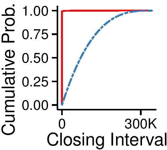
(a) Closing Interval Distribution (ArXiv)

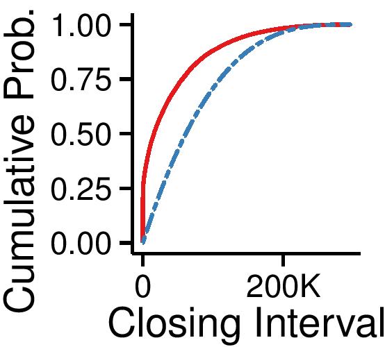
(b) Closing Interval Distribution (Email)

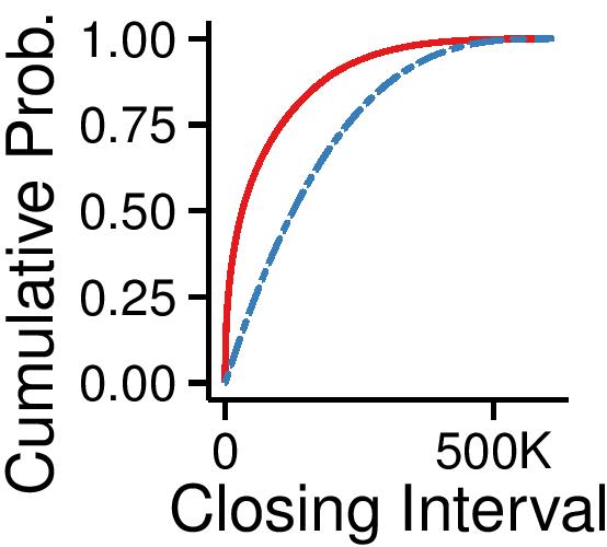
(c) Closing Interval Distribution (Facebook)

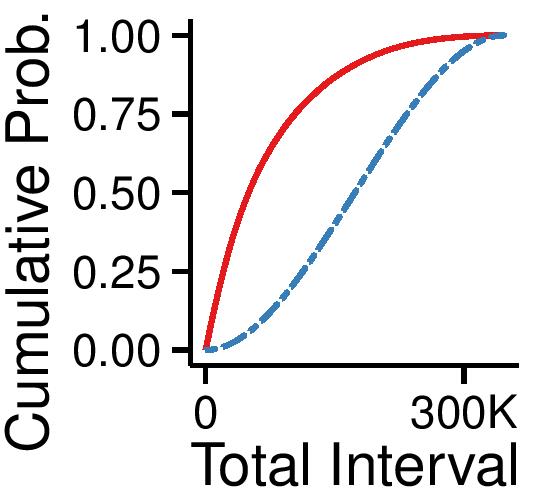
(d) Total Interval Distribution (ArXiv)

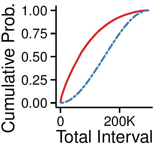
(e) Total Interval Distribution (Email)

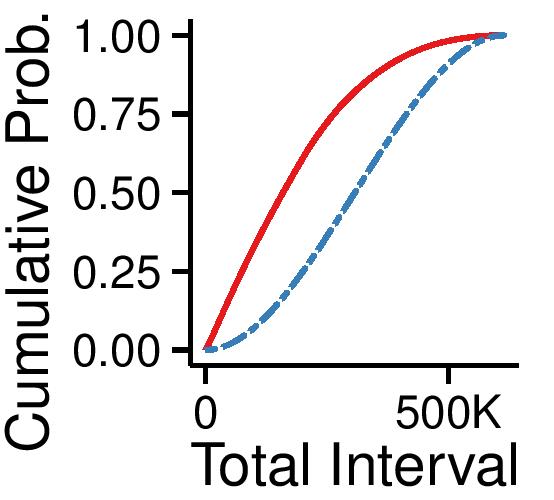
(f) Total Interval Distribution (Facebook)

Figure 2: Temporal locality in triangle formation. Closing and total intervals tend to be shorter in real graph streams than in random ones, i.e., future edges are more likely to form triangles with recent edges than with older edges.

V Proposed Method: Waiting-Room Sampling

In this section, we propose Waiting-Room Sampling (WRS), a single-pass streaming algorithm that exploits the temporal locality, presented in the previous section, for accurate global and local triangle counting. We first discuss the intuition behind WRS. Then, we explain the details of WRS. Lastly, we give theoretical analyses of its accuracy.

V-A Intuition behind WRS

To minimize the estimation error of triangle counts, we minimize both the bias and variance of estimates. Reducing the variance is related to finding more triangles because, intuitively speaking, knowing more triangles is helpful to accurately estimate their count. This relation is more formally analyzed in Section V-C. Thus, the following two goals should be considered when we decide which edges to store in memory:

Goal 1. unbiased estimates of global and local triangle counts should be computed from the stored edges.

Goal 2. when a new edge arrives, it should form many triangles with the stored edges.

Uniform random sampling, such as reservoir sampling, achieves Goal 1 but fails to achieve Goal 2 ignoring the temporal locality, explained in Section IV. Storing the latest edges, while discarding the older ones, can be helpful to achieve Goal 2, as suggested by the temporal locality. However, simply discarding old edges makes unbiased estimation non-trivial.

To achieve both goals, WRS combines the two policies above. Specifically, it divides the memory space into the waiting room and the reservoir. The most recent edges are always stored in the waiting room, while the remaining edges are uniformly sampled in the reservoir using standard reservoir sampling. The waiting room enables us to achieve Goal 2 since it exploits the temporal locality by storing the latest edges, which future edges are more likely to form triangles with. On the other hand, the reservoir enables us to achieve Goal 1, as explained in detail in the following sections.

V-B Detailed Algorithm

We first explain the sampling policy of WRS. Then, we explain how to estimate the triangle counts from sampled edges. The pseudo code of WRS is given in Algorithm 1.

V-B1 Sampling Policy (Lines 9-16 of Algorithm 1)

Let $\mathcal{S}$ be the given memory space, where at most $k$ edges are stored. Let $e^{(t)}=(u,v)$ be the edge arriving at time $t\in\{1,2,...\}$. The sampling method in WRS depends on $t$ as follows (see Section A of [25] for a pictorial description):

(Case 1). If $t\leq k$, add $e^{(t)}$ to $\mathcal{S}$, which is not full yet.

(Case 2). If $t=k+1$, since $\mathcal{S}$ is full, divide $\mathcal{S}$ into the waiting room $\mathcal{W}$ and the reservoir $\mathcal{R}$ so that the latest $k\alpha$ edges (i.e., $\{e^{(k-k\alpha+1)},...,e^{(k)}\}$) are in $\mathcal{W}$ and the remaining $k(1-\alpha)$ edges (i.e., $\{e^{(1)},...,e^{(k(1-\alpha))}\}$) are in $\mathcal{R}$. The constant $\alpha$ is the relative size of the waiting room. For simplicity, we assume $k\alpha$ and $k(1-\alpha)$ are integers. Then, go to (Case 3).

(Case 3). If $t\geq k+1$, $e^{(t-k\alpha)}$, which is the oldest edge in $\mathcal{W}$, is replaced with $e^{(t)}$ (i.e., $\mathcal{W}$ is a queue with the “first in first out” mechanism). Then, with probability $p^{(t)}$, where

$$p^{(t)}:={k(1-\alpha)}/{(t-k\alpha)},$$ (1)

$e^{(t-k\alpha)}$ replaces a randomly chosen edge in $\mathcal{R}$. Otherwise, $e^{(t-k\alpha)}$ is discarded. That is, standard reservoir sampling [19] is used in $\mathcal{R}$, which ensures that each edge in $\{e^{(1)},...,e^{(t-k\alpha)}\}$ is stored in $\mathcal{R}$ with equal probability $p^{(t)}$.

In summary, when $e^{(t)}$ arrives (or after $e^{(t-1)}$ is processed), if $t\leq k+1$, then each edge in $\{e^{(1)},...,e^{(t-1)}\}$ is stored in $\mathcal{S}$ with probability $1$. If $t>k+1$, then each edge in $\{e^{(t-k\alpha)},...,e^{(t-1)}\}$ is stored in $\mathcal{S}$ (specifically in $\mathcal{W}$) with probability $1$, while each edge in $\{e^{(1)},...,e^{(t-k\alpha-1)}\}$ is stored in $\mathcal{S}$ (specifically in $\mathcal{R}$) with probability $p^{(t-1)}$.

Algorithm 1 Waiting Room Sampling (WRS)

1:(1) graph stream: $\{e^{(1)},e^{(2)},...\}$, (2) memory budget: $k$,

2:     (3) relative size of the waiting room: $\alpha$

3:(1) estimated global triangle count: $c$,

4:        (2) estimated local triangle counts: $c_{u}$ for each node $u$

5:for each new edge $e^{(t)}=(u,v)$ do

6:    for each node $w$ in $\hat{\mathcal{N}}_{u}\cap\hat{\mathcal{N}}_{v}$  do

7:         initialize $c$, $c_{u}$, $c_{v}$, and $c_{w}$ to $0$ if they have not been set

8:         increase $c$, $c_{u}$, $c_{v}$, and $c_{w}$ by $1/p_{uvw}$     

9:    if $t\leq k$ then add $e^{(t)}$ to $\mathcal{S}$ $\vartriangleright$ (Case 1)

10:    else

11:         if $t=k+1$ then

12:$\vartriangleright$ (Case 2)

13:             divide $\mathcal{S}$ into $\mathcal{W}$ and $\mathcal{R}$ as explained in Section V-B1          

14:         remove $e^{(t-k\alpha)}$ from $\mathcal{W}$ and add $e^{(t)}$ to $\mathcal{W}$ $\vartriangleright$ (Case 3)

15:         if a random number in Bernoulli($p^{(t)}$) is $1$  then

16:             replace a randomly chosen edge in $\mathcal{R}$ with $e^{(t-k\alpha)}$              

V-B2 Estimating Triangle Counts (Lines 6-8 of Algorithm 1)

Let $\hat{\mathcal{G}}=(\hat{\mathcal{V}},\hat{\mathcal{E}})$ be the sampled graph composed of the edges in $\mathcal{S}$ ($\mathcal{W}$ or $\mathcal{R}$ if $\mathcal{S}$ is divided), and let $\hat{\mathcal{N}}_{u}$ be the set of neighbors of node $u\in\hat{\mathcal{V}}$ in $\hat{\mathcal{G}}$. We use $c$ and $c_{u}$ to denote the estimates of the global triangle count and the local triangle count of node $u$, respectively, in the stream so far. That is, if we let $c^{(t)}$ and $c^{(t)}_{u}$ be $c$ and $c_{u}$ after processing $e^{(t)}$, they are the estimates of $|\mathcal{T}^{(t)}|$ and $|\mathcal{T}^{(t)}_{u}|$, respectively.

When each edge $e^{(t)}=(u,v)$ arrives, WRS first finds the triangles composed of $(u,v)$ and two edges in $\hat{\mathcal{G}}$. The set of such triangles is $\{(u,v,w):w\in\hat{\mathcal{N}}_{u}\cap\hat{\mathcal{N}}_{v}\}$. For each triangle $(u,v,w)$, WRS increases $c$, $c_{u}$, $c_{v}$, and $c_{w}$ by $1/p_{uvw}$, where $p_{uvw}$ is the probability that WRS discovers $(u,v,w)$. Then, the expected increase of the counters by each triangle $(u,v,w)$ becomes $1$, which makes the counters unbiased estimates, as shown in Theorem 1 in the following section.

The only remaining task is to compute $p_{uvw}$, the probability that WRS discovers triangle $(u,v,w)$. To this end, we divide the types of triangles depending on the arrival times of their edges, as in Definition 3. Recall that $t^{(i)}_{uvw}$ indicates the arrival time of the edge arriving $i$-th among the edges in $(u,v,w)$.

Definition 3 (Types of Triangles).

Given the maximum number of samples $k$ and the relative size of the waiting room $\alpha$, the type of each triangle $(u,v,w)$ is defined as:

$$type_{uvw}:=\begin{cases}1&\textnormal{if}\ t^{(3)}_{uvw}\leq k+1\\ 2&\textnormal{else if}\ t^{(3)}_{uvw}-t^{(1)}_{uvw}\leq k\alpha\\ 3&\textnormal{else if}\ t^{(3)}_{uvw}-t^{(2)}_{uvw}\leq k\alpha\\ 4&\textnormal{otherwise}.\\ \end{cases}$$

That is, a triangle has Type 1 if all its edges arrive early, Type 2 if its total interval is short, Type 3 if its closing interval is short, and Type 4 otherwise. The probability that each triangle is discovered by WRS (i.e., considered in line  6 of Algorithm 1) depends on its type, as formalized in Lemma 1.

Lemma 1 (Triangle Discovering Probability.).

Given the maximum number of samples $k$ and the relative size of the waiting room $\alpha$, the probability $p_{uvw}$ that WRS discovers each triangle $(u,v,w)$ is

$$p_{uvw}=\begin{cases}1&\textnormal{if}\ type_{uvw}\leq 2\\ \frac{k(1-\alpha)}{t^{(3)}_{uvw}-1-k\alpha}&\textnormal{if}\ type_{uvw}=3\\ \frac{k(1-\alpha)}{t^{(3)}_{uvw}-1-k\alpha}\times\frac{k(1-\alpha)-1}{t^{(3)}_{uvw}-2-k\alpha}&\textnormal{if}\ type_{uvw}=4\\ \end{cases}$$ (2)

Proof.

See Section B.A of [25]. ∎

Notice that no additional space is required to store the arrival times of sampled edges. This is because the type of each triangle $(u,v,w)$ and its discovering probability $p_{uvw}$ can be computed from current time $t$ and whether each edge is stored in $\mathcal{W}$ or $\mathcal{R}$ at time $t$, as explained in the proof of Lemma 1.

V-C Accuracy Analyses

We analyze the bias and variance of the estimates provided by WRS. To this end, we define $x_{uvw}$ as the increase in $c^{(t)}$ by triangle $(u,v,w)$. By lines 6-8 of Algorithm 1, $x_{uvw}$ is $1/p_{uvw}$ with its discovering probability $p_{uvw}$, and $0$ with probability $1-p_{uvw}$. Based on this concept, the unbiasedness of the estimates given by WRS is shown in Theorem 1.

Theorem 1 (‘Any time’ unbiasedness of WRS.).

If $k(1-\alpha)\geq 2$, WRS gives unbiased estimates of the global and local triangle counts at any time. That is, if we let $c^{(t)}$ and $c^{(t)}_{u}$ be $c$ and $c_{u}$ after processing $e^{(t)}$, respectively, the followings hold:

$$\mathbb{E}[c^{(t)}]=|\mathcal{T}^{(t)}|,\ \forall t\in\{1,2,...\},$$ (3)

$$\mathbb{E}[c^{(t)}_{u}]=|\mathcal{T}^{(t)}_{u}|,\ \forall u\in\mathcal{V}^{(t)},\ \forall t\in\{1,2,...\}.$$ (4)

Proof.

See Section B.B of [25]. ∎

In our variance analysis, to give a simple intuition, we focuses on

$$\tilde{\mathrm{{Var}}}[c^{(t)}] =\sum\nolimits_{(u,v,w)\in\mathcal{T}^{(t)}}\mathrm{Var}[x_{uvw}],$$ (5)

$$\tilde{\mathrm{{Var}}}[c^{(t)}_{u}] =\sum\nolimits_{(u,v,w)\in\mathcal{T}^{(t)}_{u}}\mathrm{Var}[x_{uvw}],$$ (6)

which are the variances when the dependencies in $\{x_{uvw}\}_{(u,v,w)\in\mathcal{T}^{(t)}}$ are ignored. Specifically, we show how the temporal locality, explained in Section IV, is related to reducing $\tilde{\mathrm{{Var}}}[c^{(t)}]$ and $\tilde{\mathrm{{Var}}}[c^{(t)}_{u}]$.

From $\mathrm{Var}[x_{uvw}]=\mathbb{E}[x_{uvw}^{2}]-\left(\mathbb{E}[x_{uvw}]\right)^{2}$, we have $\mathrm{Var}[x_{uvw}]=(1/p_{uvw})-1$. From Eq. (2), if $k(1-\alpha)\geq 2$,

$$\mathrm{Var}[x_{uvw}]=\\ \begin{cases}0&\textnormal{if}\ type_{uvw}\leq 2\\ \frac{t^{(3)}_{uvw}-1-k\alpha}{k(1-\alpha)}-1&\textnormal{if}\ type_{uvw}=3\\ \frac{t^{(3)}_{uvw}-1-k\alpha}{k(1-\alpha)}\times\frac{t^{(3)}_{uvw}-2-k\alpha}{k(1-\alpha)-1}-1&\textnormal{if}\ type_{uvw}=4.\end{cases}$$ (7)

Compared to Triest-IMPR [18], where $\mathrm{Var}[x_{uvw}]=0$ if $type_{uvw}=1$ and $\mathrm{Var}[x_{uvw}]=\frac{t^{(3)}_{uvw}-1}{k}\times\frac{t^{(3)}_{uvw}-2}{k-1}-1$ otherwise, WRS reduces the variance regarding the triangles of Type 2 or 3, as formalized in Lemma 2, while WRS increases the variance regarding the triangles of Type 4.

Lemma 2 (Comparison of Variances).

For each triangle $(u,v,w)$, $\mathrm{Var}[x_{uvw}]$ is smaller in WRS than in Triest-IMPR [18], i.e.,

$$\mathrm{Var}[x_{uvw}]<\frac{t^{(3)}_{uvw}-1}{k}\times\frac{t^{(3)}_{uvw}-2}{k-1}-1$$ (8)

if any of the following conditions are satisfied:

$type_{uvw}=2$

$type_{uvw}=3$ and $t^{(3)}_{uvw}>1+\frac{\alpha}{1-\alpha}k$

$type_{uvw}=3$ and $\alpha<0.5$.

Proof.

See Section B.C of [25]. ∎

Therefore, the superiority of WRS in terms of small $\tilde{\mathrm{{Var}}}[c^{(t)}]$ and $\tilde{\mathrm{{Var}}}[c^{(t)}_{u}]$ depends on the distribution of the types of triangles in real graph streams. In the experiment section, we show that the triangles of Type 2 or 3 are abundant enough in real graph streams, as suggested by the temporal locality, so that WRS is more accurate than Triest-IMPR.

VI Experiments

We designed experiments to answer the following questions:

Q1. Accuracy: How accurately does WRS estimate global and local triangle counts?

Q2. Illustration of Theorems: Does WRS give unbiased estimates with variances smaller than its competitors’?

Q3. Scalability: How does WRS scale with the number of edges in input streams?

VI-A Experimental Settings

Machine: We ran all experiments on a PC with a 3.60GHz Intel i7-4790 CPU and 32GB memory.

Data: The real graph streams used in our experiments are summarized in Table II. See Section D of [25] for the descriptions of them. In all the streams, edges were streamed in the order by which they are created.

TABLE II: Summary of real-world graph streams.

Name	# Nodes	# Edges	Summary
ArXiv	$30,565$	$346,849$	Citation network
Facebook	$61,096$	$614,797$	Friendship network
Email	$86,978$	$297,456$	Email network
Youtube	$3,181,831$	$7,505,218$	Friendship network
Patent	$3,774,768$	$16,518,947$	Citation network

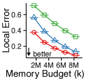
(a) Patent (Local)

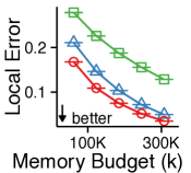
(b) Email (Local)

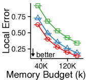
(c) Facebook (Local)

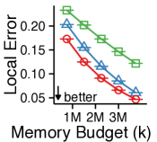
(d) Youtube (Local)

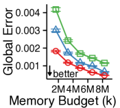
(e) Patent (Global)

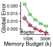
(f) Email (Global)

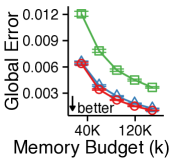
(g) Facebook (Global)

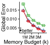
(h) Youtube (Global)

Figure 3: WRS is accurate. M: million, K: thousand. In all the datasets, WRS is most accurate in global and local triangle counting regardless of memory budget $k$.

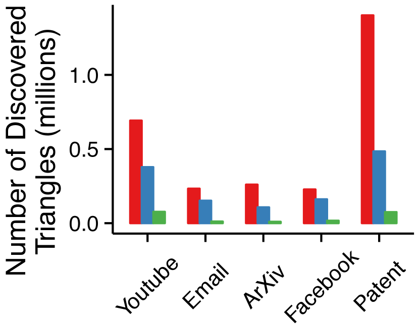
Figure 4: The sampling scheme of WRS is effective. WRS discovers up to $2.9\times$ more triangles than the second best method, in the same streams. $k$ is set to $10\%$ of the number of the edges in each dataset.

Implementations: We compared WRS to Triest-IMPR [18] and MASCOT [17], which are single-pass streaming algorithms estimating both global and local triangle counts with a limited memory budget. We implemented all the methods in Java, and in all of them, we stored sampled edges in the adjacency list format. In WRS, the relative size $\alpha$ of the waiting room was set to $0.1$ unless otherwise stated (see Section E.B of [25] for the effect of $\alpha$ on the accuracy).

Evaluation measures: To measure the accuracy of global and local triangle counting, we used the following metrics:

Global Error: Let $x$ be the number of the global triangles at the end of the input stream and $\hat{x}$ be an estimated value of $x$. Then, the global error is $|x-\hat{x}|/(x+1)$.

Local Error [17]: Let $x_{u}$ be the number of the local triangles of each node $u\in\mathcal{V}$ at the end of the input stream and $\hat{x}_{u}$ be its estimate. Then, the local error is

$$\frac{1}{|\mathcal{V}|}\sum\nolimits_{u\in\mathcal{V}}\frac{|x_{u}-\hat{x}_{u}|}{x_{u}+1}.$$

VI-B Q1. Accuracy

Figures 1(b) and 4 show the accuracies of the considered methods in the real graph streams with different memory budgets $k$. Each evaluation metric was computed $1,000$ times for each method, and the average was reported with an error bar indicating the estimated standard error. In all the datasets, WRS was most accurate in global and local triangle counting, regardless of memory budgets. The accuracy gain was especially high in the ArXiv and Patent datasets, which showed the strongest temporal locality. In the ArXiv dataset, for example, WRS gave up to 47% smaller local error and 40% smaller global error than the second best method.

WRS was more accurate since its estimates were based on more triangles. Due to its effective sampling scheme, WRS discovered up to $2.9\times$ more triangles than its competitors while processing the same streams, as shown in Figure 4.

VI-C Q2. Illustration of Theorems

We ran experiments illustrating our analyses in Section V-C. Figure 1(c) shows the distributions of $10,000$ estimates of the global triangle count in the ArXiv dataset obtained by each method. We set $k$ to the $10\%$ of the number of edges in the dataset. The average of the estimates of WRS was close to the true triangle count. Moreover, the estimates of WRS had smaller variance than those of the competitors. These results are consistent with Theorem 1 and Lemma 2.

VI-D Q3. Scalability

We measured how the running time of WRS scales with the number of edges in input streams. To measure the scalability independently of the speed of input streams, we measured the time taken by WRS to process all the edges ignoring the time taken to wait for the arrivals of edges. Figure 1(a) shows the results in graph streams that we created by sampling different numbers of edges in the ArXiv dataset. The running time of WRS scaled linearly with the number of edges. That is, the time taken by WRS to process each edge was almost constant regardless of the number of edges arriving so far.

VII Conclusion

We propose WRS, a single-pass streaming algorithm for global and local triangle counting. WRS divides the memory space into the waiting room, where the latest edges are stored, and the reservoir, where the remaining edges are uniformly sampled. By doing so, WRS exploits the temporal locality in real dynamic graph streams, while giving unbiased estimates. Specifically, WRS has the following strengths:

Fast and ‘any time’: WRS scales linearly with the number of edges in input graph streams, and it gives estimates at any time while input streams grow (Figure 1(a)).

Effective: estimation error in WRS is up to $47\%$ smaller than those in the best competitors (Figures 1(b) and 4).

Theoretically sound: WRS gives unbiased estimates with small variances under the temporal locality (Theorem 1, Lemma 2 and Figure 1(c)). Reproducibility: The code and data we used in the paper are available at http://www.cs.cmu.edu/~kijungs/codes/wrs/.

Acknowledgments. We thank Prof. Christos Faloutsos and Mr. Jisu Kim from Carnegie Mellon University for fruitful discussions. This material is based upon work supported by the National Science Foundation under Grant No. CNS-1314632 and IIS-1408924. Research was sponsored by the Army Research Laboratory and was accomplished under Cooperative Agreement Number W911NF-09-2-0053. Kijung Shin was supported by KFAS Scholarship. Any opinions, findings, and conclusions or recommendations expressed in this material are those of the author(s) and do not necessarily reflect the views of the National Science Foundation, or other funding parties. The U.S. Government is authorized to reproduce and distribute reprints for Government purposes notwithstanding any copyright notation here on.

References

- [1] M. McPherson, L. Smith-Lovin, and J. M. Cook, “Birds of a feather: Homophily in social networks,” Annual review of sociology, vol. 27, no. 1, pp. 415–444, 2001.
- [2] S. Wasserman and K. Faust, Social network analysis: Methods and applications. Cambridge university press, 1994, vol. 8.
- [3] D. J. Watts and S. H. Strogatz, “Collective dynamics of ‘small-world’networks,” nature, vol. 393, no. 6684, pp. 440–442, 1998.
- [4] M. E. Newman, “The structure and function of complex networks,” SIAM review, vol. 45, no. 2, pp. 167–256, 2003.
- [5] L. Becchetti, P. Boldi, C. Castillo, and A. Gionis, “Efficient algorithms for large-scale local triangle counting,” TKDD, vol. 4, no. 3, p. 13, 2010.
- [6] J.-P. Eckmann and E. Moses, “Curvature of co-links uncovers hidden thematic layers in the world wide web,” PNAS, vol. 99, no. 9, pp. 5825–5829, 2002.
- [7] K. Shin, T. Eliassi-Rad, and C. Faloutsos, “Corescope: Graph mining using k-core analysis - patterns, anomalies and algorithms,” in ICDM, 2016.
- [8] Z. Bar-Yossef, R. Kumar, and D. Sivakumar, “Reductions in streaming algorithms, with an application to counting triangles in graphs,” in SODA, 2002.
- [9] J. Shun and K. Tangwongsan, “Multicore triangle computations without tuning,” in ICDE, 2015.
- [10] J. Kim, W.-S. Han, S. Lee, K. Park, and H. Yu, “Opt: A new framework for overlapped and parallel triangulation in large-scale graphs,” in SIGMOD, 2014.
- [11] X. Hu, Y. Tao, and C.-W. Chung, “I/o-efficient algorithms on triangle listing and counting,” TODS, vol. 39, no. 4, p. 27, 2014.
- [12] S. Arifuzzaman, M. Khan, and M. Marathe, “Patric: A parallel algorithm for counting triangles in massive networks,” in CIKM, 2013.
- [13] S. Suri and S. Vassilvitskii, “Counting triangles and the curse of the last reducer,” in WWW, 2011.
- [14] H.-M. Park, F. Silvestri, U. Kang, and R. Pagh, “Mapreduce triangle enumeration with guarantees,” in CIKM, 2014.
- [15] H.-M. Park, S.-H. Myaeng, and U. Kang, “Pte: Enumerating trillion triangles on distributed systems,” in KDD, 2016.
- [16] K. Kutzkov and R. Pagh, “On the streaming complexity of computing local clustering coefficients,” in WSDM, 2013.
- [17] Y. Lim and U. Kang, “Mascot: Memory-efficient and accurate sampling for counting local triangles in graph streams,” in KDD, 2015.
- [18] L. De Stefani, A. Epasto, M. Riondato, and E. Upfal, “Triest: Counting local and global triangles in fully-dynamic streams with fixed memory size,” in KDD, 2016.
- [19] J. S. Vitter, “Random sampling with a reservoir,” TOMS, vol. 11, no. 1, pp. 37–57, 1985.
- [20] C. E. Tsourakakis, U. Kang, G. L. Miller, and C. Faloutsos, “Doulion: counting triangles in massive graphs with a coin,” in KDD, 2009.
- [21] M. Jha, C. Seshadhri, and A. Pinar, “A space efficient streaming algorithm for triangle counting using the birthday paradox,” in KDD, 2013.
- [22] A. Pavan, K. Tangwongsan, S. Tirthapura, and K.-L. Wu, “Counting and sampling triangles from a graph stream,” PVLDB, vol. 6, no. 14, pp. 1870–1881, 2013.
- [23] K. Kutzkov and R. Pagh, “Triangle counting in dynamic graph streams,” in SWAT, 2014.
- [24] M. N. Kolountzakis, G. L. Miller, R. Peng, and C. E. Tsourakakis, “Efficient triangle counting in large graphs via degree-based vertex partitioning,” in WAW, 2010.
- [25] K. Shin, “Wrs: Waiting room sampling for accurate triangle counting in real graph streams (supplementary document),” Available online: http://www.cs.cmu.edu/~kijungs/codes/wrs/supple.pdf, 2017.