The life cycle of starbursting circumnuclear gas discs

Abstract

High-resolution observations from the sub-mm to the optical wavelength regime resolve the central few 100 pc region of nearby galaxies in great detail. They reveal a large diversity of features: thick gas and stellar discs, nuclear starbursts, in- and outflows, central activity, jet interaction, etc. Concentrating on the role circumnuclear discs play in the life cycles of galactic nuclei, we employ 3D adaptive mesh refinement hydrodynamical simulations with the Ramses code to self-consistently trace the evolution from a quasi-stable gas disc, undergoing gravitational (Toomre) instability, the formation of clumps and stars and the disc’s subsequent, partial dispersal via stellar feedback. Our approach builds upon the observational finding that many nearby Seyfert galaxies have undergone intense nuclear starbursts in their recent past and in many nearby sources star formation is concentrated in a handful of clumps on a few 100 pc distant from the galactic centre. We show that such observations can be understood as the result of gravitational instabilities in dense circumnuclear discs. By comparing these simulations to available integral field unit observations of a sample of nearby galactic nuclei, we find consistent gas and stellar masses, kinematics, star formation and outflow properties. Important ingredients in the simulations are the self-consistent treatment of star formation and the dynamical evolution of the stellar distribution as well as the modelling of a delay time distribution for the supernova feedback. The knowledge of the resulting simulated density structure and kinematics on pc scale is vital for understanding inflow and feedback processes towards galactic scales.

1 Introduction

Circumnuclear gas discs are ubiquitously observed in the central regions of many classes of galaxies. Interacting systems and Ultra-luminous Infrared Galaxies (ULIRGS, Downes & Solomon, 1998; Medling et al., 2014) have especially attracted the interest of many researchers. The detected discs in these systems typically have dimensions of several hundred parsecs, gas masses of the order of $10^{8}$ to $10^{10}\,$M_⊙ and ratios of rotational velocity to velocity dispersion of $v/\sigma$ between 1 and 5 (Medling et al., 2014). It is found that a large fraction of the coexisting stellar discs are consistent with being formed recently (<30 Myr) within the gaseous discs. We will especially concentrate on the case of active galaxies, where we are interested in investigating the interplay between nuclear disc evolution and nuclear activity, as well as their mutual relation. According to the so-called Unified Scheme of Active Galactic Nuclei (AGN) (Miller & Antonucci, 1983; Antonucci, 1993; Urry & Padovani, 1995) these objects are thought to be powered by accretion onto their central supermassive black hole. Angular momentum conservation of the infalling gas leads to the formation of a viscously heated accretion disc. The latter can easily outshine the stars of the whole galaxy and illuminates a larger gas and dust reservoir on parsec scale, the so-called dusty, molecular torus (e. g.  Krolik & Begelman, 1988; Nenkova et al., 2002; Hönig et al., 2006; Schartmann et al., 2008; Stalevski et al., 2012; Wada, 2012; Siebenmorgen et al., 2015; Wada et al., 2016). Mass transfer onto and through these structures is often provided from an adjacent circumnuclear disc or mini-spiral (e. g.  Prieto et al., 2005; Hicks et al., 2009; Davies et al., 2014; Durré & Mould, 2014) which typically reaches out to several hundreds of parsecs in nearby galactic nuclei. These discs are found to be made up of a multi-phase mixture of gas and dust at various temperatures and various stages of ionisation arising from shocks, star formation (SF) and the radiation from the active nucleus as well as stars. Additional frequently observed components are outflows, partly in the form of collimated, highly powerful jets, but also in wide-angle, lower velocity, but high mass loaded winds. The strengths of the various phenomena differ from source to source. All of these components are at the limits of resolution, not just of our largest telescopes and best instrumentation, but also of hydrodynamical codes that deal with their time evolution.

Observationally, such systems have e. g. been investigated by Davies et al. (2007), Hicks et al. (2013) and Lin et al. (2016), concentrating on a sample of nearby Seyfert galaxies. They find a much higher rate of circumnuclear discs in active galaxies compared to their inactive sample. Such studies with integral field units at the largest available telescopes with resolutions of a few parsec find that gaseous and stellar structures are often cospatial and share similar kinematics, indicating that stars may have formed in-situ from the gas discs. Morphologies range from smooth, star forming discs and mini-spirals (Prieto et al., 2005) over star formation concentrated in clumps (Durré & Mould, 2014) to very disturbed filamentary outflowing structures (Durré et al., 2017) and are readily visible in dust extinction maps as well (Prieto et al., 2005, 2014). Most of these sources do not show any signs of recent merging activity that could provide the necessary torques to transfer gas towards the central region. Hence the discs / mini-spirals are thought to be formed mostly by secular evolution processes (Orban de Xivry et al., 2011; Maciejewski, 2004a, b), driving gas into the nuclear region (typically up to several hundred parsecs), e. g. via bars (Sakamoto et al., 1999; Sheth et al., 2005; Krumholz & Kruijssen, 2015). After enough gas has been accumulated, the discs become gravitationally unstable (Toomre, 1964; Behrendt et al., 2015). This is the starting point of our simulations, which we approximate with idealised, marginally (Toomre) unstable discs.

Theoretically, the formation and evolution of circumnuclear gas discs has mainly been studied within simulations of mergers of gas-rich galaxies (in isolation and within cosmological frameworks). Gravitational torques are able to remove angular momentum from shocked interstellar gas, leading to infall. Cosmological zoom simulations are nowadays able to follow these processes down to the formation of circumnuclear discs similar to the ones observed on several 100 parsecs scale (Levine et al., 2008; Hopkins & Quataert, 2010). Due to their violent past, many of these discs are warped and can have complex kinematics, partly decoupled from the rest of the galaxy (Barnes, 2002). These discs typically grow inside-out and disc formation can take place over a long period of time, due to infalling tidal tails. Roškar et al. (2015) find that directly after the merger, a strong starburst event evacuates the central region surrounding the supermassive black hole (SMBH), but a circumnuclear disc of several 100 pc size reforms on a time scale of roughly 10 Myr. Most of these studies concentrate on the effect of such a gas disc on the evolution and the in-spiral of a black hole binary, following the recent merging event (e. g.  Chapon et al., 2013).

The dynamical state of (starbursting) circumnuclear discs in nearby active galaxies has been studied by Fukuda et al. (2000), Wada & Norman (2002) and Wada et al. (2009). They find that supernova (SN) feedback under starburst conditions turns a rotationally supported thin disc into a turbulent, clumpy, geometrically thick toroidal structure on tens of parsecs scale with significant contributions to the total obscuration properties. The generated turbulence efficiently drives gas towards the SMBH. For the case of an already activated galactic nucleus, a radiation-pressure driven fountain flow – enabled by the direct radiation pressure from a central source – can also lead to a geometrically thick distribution and drive a significant outflow along the symmetry axis (Wada, 2012, 2015) and is able to describe some observed properties of nearby Seyfert galaxies (Schartmann et al., 2014). The combination of SN and central radiation feedback enabled a good description of the observable properties of the very well-studied Circinus galaxy (Wada et al., 2016).

Our approach is complementary to this set of simulations. In this first publication, we start by characterising self-consistent self-gravitating hydrodynamical simulations of Toomre unstable circumnuclear discs. Spanning a full starburst cycle, we study their gravitational instability, star forming properties and the driving of winds towards galactic scales. Such simulations – constrained by the mentioned observations – will allow us to derive a consistent picture of the mass budget of these systems concerning star formation and in- and outflows driven by the starburst. The tens of parsecs scale vicinity of SMBHs is not only important for fuelling the central putative molecular, dusty torus (e. g.  Schartmann et al., 2008, 2014), but can also provide a fraction of the necessary obscuration (Hicks et al., 2009; Prieto et al., 2014; Wada & Norman, 2002; Wada, 2015), which in turn is important for assessing the efficiency of SMBH feedback towards galactic scales.

We present our physical model, parameters and assumptions in Sect. 2, discuss the evolution of its hydrodynamical realisation and of a parameter study in Sect. 3 and compare the results to observations (Sect. 4). We critically discuss our obtained results in Sect. 5, before we conclude our analysis in Sect. 6.

2 The physical model and its numerical representation

In this first simulation series, we include only a subset of physical processes and a simple initial condition guided by observations. This will form the basis of our investigation of the life cycles and dynamics of gas and stars in circumnuclear discs in the nuclei of nearby active galaxies. Subsequently adding more physical processes will give us a detailed understanding of their internal workings.

2.1 The initial gas disc setup and the background potential

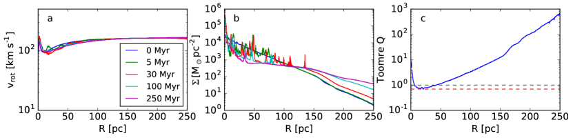
Figure 1: Azimuthally averaged rotation velocity (a), surface density (b) and Toomre Q parameter (c) of the disc at various evolutionary stages (see legend). In panel (c), only the initial condition is shown. The centre reaches high values of the Toomre Q parameter, which is followed by a marginally unstable region (up to several ten parsecs distance from the centre) that forms stars and turns the initially smooth into a clumpy disc, whereas the outer region remains stable and smooth.

The most common feature of the IFU observations are nuclear, rotating disc structures. Hence, in our basic model, we assume that there is a pre-existing gas disc with a radially exponential surface density distribution with a scaling length of 30 pc, following the observations presented by Hicks et al. (2009). It is rotationally supported in the radial direction and in approximate vertical hydrostatic equilibrium with a background potential (BH and stellar bulge, see below) and the self-gravity of the disc itself. The disc temperature is set to $T_{\mathrm{disc,ini}}=10^{4}$ K. The latter is thought to replace an unresolved micro-turbulent pressure floor. Such a micro-turbulent pressure floor can be thought of as arising from the transfer of gravitational potential energy from the accretion of gas towards the centre (Klessen & Hennebelle, 2010, see discussion in Sect. 5.5). In the limit of small disc masses around a point mass, this setup leads to a vertical Gaussian distribution of the gas density. In the self-gravity limit when the gas disc dominates over the central point source, a $\sec^{2}$ density distribution results. Our case is intermediate and partially dominated by the extended background potential and we numerically calculate the vertical structure of the disc. It is surrounded by a hot atmosphere with $T_{\mathrm{atm,ini}}=10^{6}$ K in approximate hydrostatic equilibrium with the BH, bulge and gas self-gravity potential. Being interested in the local galaxy population, we set the central supermassive black hole mass to $M_{\mathrm{BH}}=10^{7}\,$M_⊙, which is implemented as a Gaussian background potential with a full width at half maximum (FWHM) of 2 pc. The second component is the (old) stellar bulge that dominates the background potential. Its mass is set to $M_{\mathrm{bulge}}=8.5\times 10^{9}\,$M_⊙, derived following the scaling relation between central supermassive black holes and their stellar bulge masses given by Häring & Rix (2004). We model it with a spherical Hernquist (Hernquist, 1990) potential with a half-mass radius of $r_{\mathrm{h}}^{\mathrm{bulge}}=820$ pc. The latter has been approximated following Berg et al. (2014, Fig. 3). Together with the self-gravity of the gas, this background potential results in a flat rotation curve over most part of our computational domain (Fig. 1a), as typically derived from observations of nearby AGN (e. g.  Davies et al., 2007; Hicks et al., 2009). The size of the initial disc is chosen to be a few times the scale length of the observed discs and similar to the field of view of the IFU and spectral observations which will be used to compare our results to. The computational domain is a cube with a side length of 2048 pc. A summary of the model parameters is given in Table 1.

Table 1: Model parameters of the simulations.

$M_{\mathrm{BH}}$	$10^{7}\,$M⊙	$M_{\mathrm{gas,ini}}$	$10^{8}\,$M⊙
$M_{\mathrm{bulge}}$	$8.5\times 10^{9}\,\mathrm{M}_{\odot}$	$r_{\mathrm{h}}^{\mathrm{bulge}}$	820 pc
$T_{\mathrm{disc,ini}}$	$10^{4}$ K	$T_{\mathrm{atm,ini}}$	$10^{6}$ K
$\Delta x_{\mathrm{box}}$	2048 pc	$l_{\mathrm{disc}}$	30 pc
$n_{\mathrm{SF}}$	$2\times 10^{6}\,\mathrm{cm}^{-3}$	$\epsilon_{\mathrm{SF}}$	0.02%
$\eta_{\mathrm{SN}}$	0.1	$E_{\mathrm{SN}}$	$10^{51}$ erg
$m^{*}_{\mathrm{SN}}$	10 M⊙	$m_{*}$	100 M⊙
$m^{\mathrm{SN}}_{\mathrm{threshold}}$	1000 M⊙	$R^{\mathrm{max}}_{\mathrm{bubble}}$	10 pc

$M_{\mathrm{BH}}$ is the central black hole mass, $M_{\mathrm{gas,ini}}$ is the total initial gas mass (disc plus atmosphere), $M_{\mathrm{bulge}}$ is the mass of the (old) stellar bulge, $r_{\mathrm{h}}^{\mathrm{bulge}}$ its half-mass radius, $T_{\mathrm{disc,ini}}$ the initial temperature of the disc, $T_{\mathrm{atm,ini}}$ the initial temperature of the atmosphere, $\Delta x_{\mathrm{box}}$ the size of the computational domain, $l_{\mathrm{disc}}$ the scale length of the exponential gas disc, $n_{\mathrm{SF}}$ is the hydrogen number density threshold for star formation, $\epsilon_{\mathrm{SF}}$ is the star formation efficiency per free-fall time, $\eta_{\mathrm{SN}}$ is the fraction of stellar mass that goes into supernovae and $E_{\mathrm{SN}}$ is the assumed energy injected per SN and $m^{*}_{\mathrm{SN}}$ is the assumed mass of a SN progenitor star, $m_{*}$ is the typical mass of a stellar population / star cluster, $m^{\mathrm{SN}}_{\mathrm{threshold}}$ is the gas mass threshold to determine the SN bubble radius, $R^{\mathrm{max}}_{\mathrm{bubble}}$ is the maximum SN bubble radius.

2.2 Numerical hydrodynamics, self-gravity and adaptive mesh refinement

We solve the system of hydrodynamical equations and the Poisson equation with the help of the Ramses (Teyssier, 2002) code, which uses a second-order Godunov-type hydrodynamical adaptive mesh refinement (AMR) scheme with an octree-based data structure. The solver proposed by Harten et al. (1983, HLL Riemann solver) is used to calculate the solution to the Riemann problem. The complex physics of star formation (SF) and stellar feedback necessitate a very high spatial resolution. We adopt a quasi-Lagrangian AMR strategy and refine a cell up to a maximum refinement level whenever its mass (including the old stellar bulge and the central SMBH) exceeds a given threshold mass for the respective level. We furthermore require that the Jeans length is resolved by at least 5 grid cells. This refinement strategy enables us to prevent artificial fragmentation (Truelove et al., 1997), allows us to efficiently resolve clump formation and evolution and concentrates the resolution to the central region, but still allows us to trace potential outflows towards several 100 pc scales. A base grid with a cell size of 32 pc is chosen and with 7 levels of refinement we reach a smallest grid size of 0.25 pc in the dense structures close to the midplane of the disc. The interactions of the stellar particles within the potential are calculated with a particle-mesh technique.

2.3 Numerical treatment of star formation

In this work, we follow the definition of Krumholz & McKee (2005) for the dimensionless star formation rate per free-fall time $\epsilon_{\mathrm{SF}}$ as the fraction of the mass (above a certain density threshold $\rho_{\mathrm{SF}}$) of a grid cell that it converts into stars per free-fall time at this density: $\epsilon_{\mathrm{SF}}=\dot{M}_{*}\,/\,[M(\geq\rho_{\mathrm{SF}})\,/\,t_{\mathrm{ff}}(\rho_{\mathrm{SF}})]$, where $\dot{M}_{*}$ is the star formation rate, $M(\geq\rho_{\mathrm{SF}})$ is the mass in the volume where $\rho\geq\rho_{\mathrm{SF}}$ and the free-fall time of a sphere is given by $t_{\mathrm{ff}}=\sqrt{3\,\pi\,/(32\,G\,\rho)}$ and $\rho$ is the local gas density within the cell. For Giant Molecular Clouds (GMCs) $\epsilon_{\mathrm{SF}}$ was observationally found to be roughly 0.01 (Zuckerman & Evans, 1974). Krumholz & Tan (2007) find no evidence for a transition from slow to rapid star formation up to densities of $n_{\mathrm{H}}\approx 10^{5}\,\mathrm{cm}^{-3}$, but the compiled observational data is consistent with $\epsilon_{\mathrm{SF}}$ of a few per cent, independent of gas density.

To model star formation in the code, we use a modified version of the Ramses standard recipe (Rasera & Teyssier, 2006), which we will only briefly describe in the following. Star formation is treated in our implementation on a cell-by-cell basis and takes place, whenever the gas density exceeds the threshold density for star formation ($\rho>\rho_{\mathrm{SF}}$). Within this numerical recipe, both, $\rho_{\mathrm{SF}}$ as well as $\epsilon_{\mathrm{SF}}$ are free parameters. This threshold density is set such to (i) prevent the smooth initial disc from forming stars and only allow dense collapsing clumps created by Toomre instability to form stars and (ii) be below the density threshold at which the artificial pressure floor is activated (see Sect. 2.6), which is resolution dependent. Due to the already very high densities of the initial condition and the limited resolution, this results in a narrow possible range and a star formation density threshold of $n_{\mathrm{H}^{*}}=2\times 10^{6}\,\mathrm{cm}^{-3}$ was chosen, in accordance with Lupi et al. (2015). The high spatial resolution in these simulations concentrating on galactic nuclei allow to resolve the gravitational collapse up to these high densities. In order to reach a reasonable match with the starburst Kennicutt-Schmitt relation by Daddi et al. (2010) on global scales (see discussion in Sect. 4.1), we adjust the star formation efficiency. The latter criterion links the two SF parameters and is identical to requiring a global gas depletion time scale in accordance with observations and a value of $\epsilon_{\mathrm{SF}}=0.02\%$ is found. Those cells fulfilling the criteria form stars according to a Schmidt-like star formation law: $\dot{\rho}_{*}=\epsilon_{\mathrm{SF}}\,\rho\,/\,t_{\mathrm{ff}}$, where $\rho$ is the local gas density. This is realised with stellar N-body particles, which have an integer multiple $N$ of a fixed threshold mass $m_{*}$, set to 100 M_⊙ (see Table 1). Each stellar particle hence corresponds to a stellar population or star cluster. $N$ is determined following a Poisson probability distribution function (Rasera & Teyssier, 2006) in order to accurately sample the required star formation rate. Whenever a star particle is born, we update the fluid and the star particle quantities in a conservative way, the latter take over the velocity of the gas cell and they are put at the centre of their parent cell. Care is also taken that no more than 50% of the gas is consumed in new-born stars within a single star formation event.

It should be noted that such an approach is complementary to models which derive $\epsilon_{\mathrm{SF}}$ from first principles, like e. g. Krumholz & McKee (2005), but the treatment is in line with the finding by Krumholz et al. (2012) that star formation follows a simple volumetric law, depending only on local gas conditions.

2.4 Treatment of supernova feedback

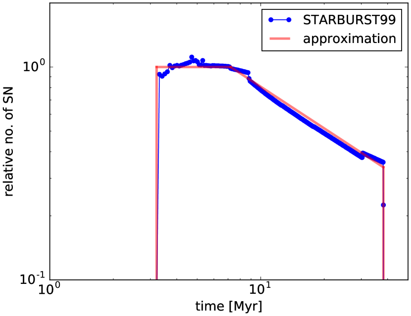
Figure 2: Normalised SN delay time distribution adapted from a Starburst99 simulation. The red line shows the analytical approximation used in the simulations.

For the supernova feedback, we use a modified version of the Ramses implementation by Dubois & Teyssier (2008). Star particles are evolved with a particle-in-cell method and a fraction $\eta_{\mathrm{SN}}$ of their mass will be recycled into the ISM during supernova (SN) explosions, whereas the remaining part is locked in long-lived stars. Assuming a Salpeter initial mass function (IMF) leads to a SN yield of roughly 10%. Assuming a typical progenitor star mass of $10\,$M_⊙, each star particle – which we identify with a stellar population or star cluster – will cause one SN explosion per $m_{*}$ of star particle mass over time. Already during the numerical star formation process described in Sect. 2.3, we randomly determine a delay time for each prospective SN explosion, following a SN delay time distribution, which is the time between the birth of the stellar particle and the detonation of one of its SN. The delay time distribution is shown in Fig. 2. The blue symbols represent the normalised SN rate expected from a coeval stellar population as derived from a Starburst99 (Leitherer et al., 1999, 2014) simulation. The red curve corresponds to the analytical approximation used in our simulations. SN explosions in this scheme should be thought of as the combined energy and mass input from the stellar wind phase and the actual SN explosion. For the most massive stars, the energy input in the stellar wind phase can be of similar order or even exceeding the SN explosion itself (e. g.  Fierlinger et al., 2016). Uncertainties in the total ejected SN energies are expected to be at least similarly large.

As soon as a star particle is eligible for an SN explosion, we initiate the following procedure:

1. The hydrodynamical state vector is averaged over a given, initial SN bubble radius ($R_{\mathrm{bubble}}$). The latter is set to two cell diameters, in order to be at the same time resolved and smaller than typical structures found in the simulations. If the total mass within this radius falls short of a mass threshold $m^{\mathrm{SN}}_{\mathrm{threshold}}$, we increase the bubble radius stepwise by 10% up to a maximum radius $R^{\mathrm{max}}_{\mathrm{bubble}}$. This procedure prevents tiny time steps in regions of low gas densities. In these low density regions, SN bubbles would grow to larger sizes on short timescale anyway, validating our approach.

2. A fraction of 50% of the total SN energy of $10^{51}$ erg is injected as thermal energy evenly distributed over the spherical bubble and 50% is injected in kinetic energy with a linearly increasing radial velocity as a function of distance from the centre of the explosion. Additionally, the SN ejecta take over the motion of their parent stellar cluster.

3. The remaining (hydrodynamical) evolution is followed self-consistently.

2.5 Gas cooling

As the focus of this work is on the dynamical evolution, we use a simplistic treatment of the chemical and thermodynamical evolution of the gas. An adiabatic equation of state with an adiabatic index of $\Gamma=5/3$ is assumed. To account for the cooling of the gas, we use one of the Ramses cooling modules, which interpolates the cooling rates within pre-computed tables for a fixed metallicity corresponding to solar abundances. The latter have been calculated using the CLOUDY photoionisation code (Ferland et al., 1998). This results in a comparable effective cooling curve to the one described in Dalgarno & McCray (1972) and Sutherland & Dopita (1993). A fraction of the gas is expected to be heated by photoelectric heating from the forming young stars. In order to save computational time, this is crudely accounted for by applying a minimum temperature cut-off at $T=10^{4}$ K (see also discussion in Sec. 5).

2.6 Additional numerical concepts

If the Jeans length becomes comparable to the grid scale, pressure gradients that stabilise the gas against collapse cannot be resolved anymore and artificial fragmentation can occur in the self-gravitating gas. To efficiently avoid this, we introduce an artificial pressure floor in addition to the temperature threshold mentioned in Sec. 2.5 (e. g.  Machacek et al., 2001; Agertz et al., 2009; Teyssier et al., 2010; Behrendt et al., 2015):

$$P\geq\frac{\rho^{2}\,G}{\pi\,\gamma}\,N^{2}\,\Delta x^{2}$$ (1)

where $P$ is the thermal pressure, $\rho$ the density of the gas, $G$ the gravitational constant, $\Delta x$ the minimum cell size, $\gamma=5/3$ the adiabatic index. This pressure floor ensures that the local Jeans length is resolved with at least $N$ grid cells. We choose $N=4$ in order to fulfil the Truelove criterion (Truelove et al., 1997) and thereby avoid artificial fragmentation throughout the simulation volume. The corresponding heating of this numerical treatment, however, does not affect the star formation described in Sect. 2.3.

3 Results of the simulations

3.1 Overall evolution of the simulation

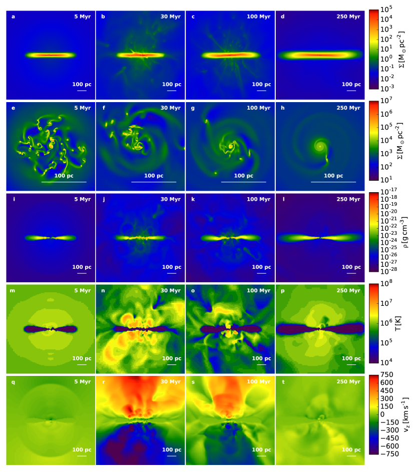
Figure 3: Evolution of the model with time. Shown are density projections along the $x$-axis (upper row), zoomed-in projections along the $z$-axis (second row), density slices (third row), temperature slices (fourth row) and vertical velocity slices (fifth row) through the $yz$-plane. Mind the different dynamic ranges and scales of the various rows. Toomre instability leads to clump formation in the self-gravitating gas disc and the subsequent starburst turns it into a three-component structure: (i) the remaining gas disc, (ii) a fountain-like flow in the central region and (iii) a hot, large-scale outflow. After the clumps have been dissolved, the SF rate decreases and the disc turns into an almost quiescent state again.

The time evolution of the gas density distribution is shown in the upper three rows of Fig. 3. Density projections along the $x$- and $z$-axis are shown in the first and second row (mind the differences in colour and physical scale). The third row shows a cut through the three-dimensional gas density distribution along a meridional plane. As mentioned in Sect. 2.1, the initial condition is marginally Toomre unstable in the central 40-50 parsec (blue line in Fig. 1c). Small perturbations due to the Cartesian grid allow the growth of unstable modes of this axisymmetric instability, which leads to the formation of a number of concentric ring-like density enhancements. The slightly higher Q-values in the very centre trigger spiral-like features. During the non-linear evolution of the instability, these rings and spiral-like structures break up into a large number of clumps. For a detailed description of this evolution we refer to Behrendt et al. (2015), where Toomre theory is studied in great detail with the aim of explaining the observed properties of gas-rich, clumpy high redshift disc galaxies. The clumps’ early evolution is governed by a complex interplay of various processes: grouping to clump clusters (Behrendt et al., 2016), clump merging, tidal interactions, (partial) dispersal and gain of mass by interaction with the diffuse gas component. After having contracted to reach the gas threshold density, star formation is triggered in their densest, central parts, leading to depletion of the gas clumps themselves. After the randomly determined delay time, the star particles recycle a fraction of their gas to the ISM within SN explosions. These energetic events drive random motions and outflows, thereby depleting the clumps further. Due to the early strong rise and extremum of the delay time distribution (Fig. 2), a three-component flow forms shortly afterwards, especially visible in the edge-on projections of the density (Fig. 3b,c) and slices (Fig. 3j,k), as well as the temperature (Fig. 3n,o) and $z$-velocity slices (Fig. 3r,s): (i) the remaining thin, high density and cold disc (at $10^{4}$ K, our minimum temperature) that shows random motions due to clump-clump interactions, (ii) a SN-driven fountain-like flow in the central, strongly star-bursting region where cold dense filaments are ejected into the hot atmosphere and partly fall back onto the disc (Fig. 3n,o), stirring additional random motion and (iii) a low-density, hot outflow that partly erodes the lifted filaments and escapes the computational domain (Fig. 3n,o and r,s). The filamentary structure during the starbursting phase is strengthened, as supernova explosions are more effective in the low, inter-filament gas, further enhancing the density contrast (Schartmann et al., 2009). Overall, this evolution results in a decrease of the clump masses, which is only partly balanced by the merging of clumps. Most of the clumps vanish within roughly 200 Myr, leading to the starvation of the intense star burst (right column of Fig. 3). Only a few clumps keep orbiting in the very centre and the system leaves the starbursting regime (see discussion in Sect. 4.1 and Fig. 11). As a consequence, the disc returns to an almost quiescent state again with a low number of SN explosions and only a hot and low density outflow remaining, that ceases soon after.

3.2 Statistical distribution of the gas

Fig. 4a shows the time evolution of the volume-weighted density probability distribution functions (PDF) for all gas cells within a sphere of 512 pc radius surrounding the centre (disregarding the edges and outer regions of the simulation box) and normalised by the total volume. The state close to the initial condition is given in dark blue. Two distinct phases can be distinguished: the power law at the lowest densities corresponds to the hot atmosphere (marked by the blue background) and the smooth initial gas disc (yellow and green background for the initial condition) can be fitted by a log-normal distribution (white thick dashed line). The evolution through Toomre instability and the non-linear clump formation leads to a change of the log-normal distribution into a broken-power law distribution with a knee at around $2\times 10^{-21}$ g cm^-3, separating the inner, clumpy disc (green background) from the Toomre stable, smooth outer disc (yellow background). Ongoing clump formation and merging extends this power-law to higher and higher densities (green data points), until stellar particles are allowed to form. The power law tail in the high density region of the PDF is expected for self-gravitating gas that can no longer be held up against gravity by turbulence (e. g.  Vázquez-Semadeni et al., 2008; Elmegreen, 2011). Around the peak of the starburst (at 30 Myr, red graph), part of the high density gas phase has been turned into stars and energy injection due to the subsequent SN explosions feeds the fountain flow and hot outflow. This results in a decrease of the volume and mass of the high density gas and a characteristic bump in the density PDF at lower densities (hatched region), replacing the hot atmosphere in hydrostatic equilibrium. The latter can be described by a log-normal distribution – which is characteristic of isothermal, supersonic turbulence (e. g.  Vazquez-Semadeni, 1994; Federrath et al., 2008) – plus a higher density power-law. The PDF at this evolutionary stage is split into a radially outflowing, in-flowing and non-moving part (Fig. 4b). This allows clearly separation of the various physical mechanisms and evolutionary states in the simulation: The remaining smooth disc (or ring) – unaffected by Toomre instability – is in radial centrifugal equilibrium and shows almost no in- or outflow motion (yellow line in Fig. 4b) between $5\times 10^{-24}$ and $2\times 10^{-21}$ g cm^-3. In the inner, clumpy part of the disc (green background), the gas is approximately equally distributed between the three kinematic states due to the random motions stirred by clump-clump interactions following gravitational instability. The bump at low densities can be identified as the wind and fountain flow driven by the starburst, which is dominated by random motions. Here, the hot outflowing gas dominates the volume filling fraction, as inflow happens in dense, compressed filaments only. With decreasing strength of the starburst (cyan line, 100 Myr; Fig. 4a), more and more high density clumps vanish and the outflow bump moves to lower densities until – in the post-starburst phase – the outflow ceases almost completely (yellow line, 250 Myr) towards the end of the simulation.

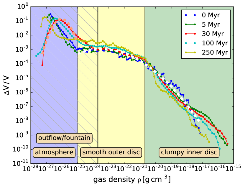
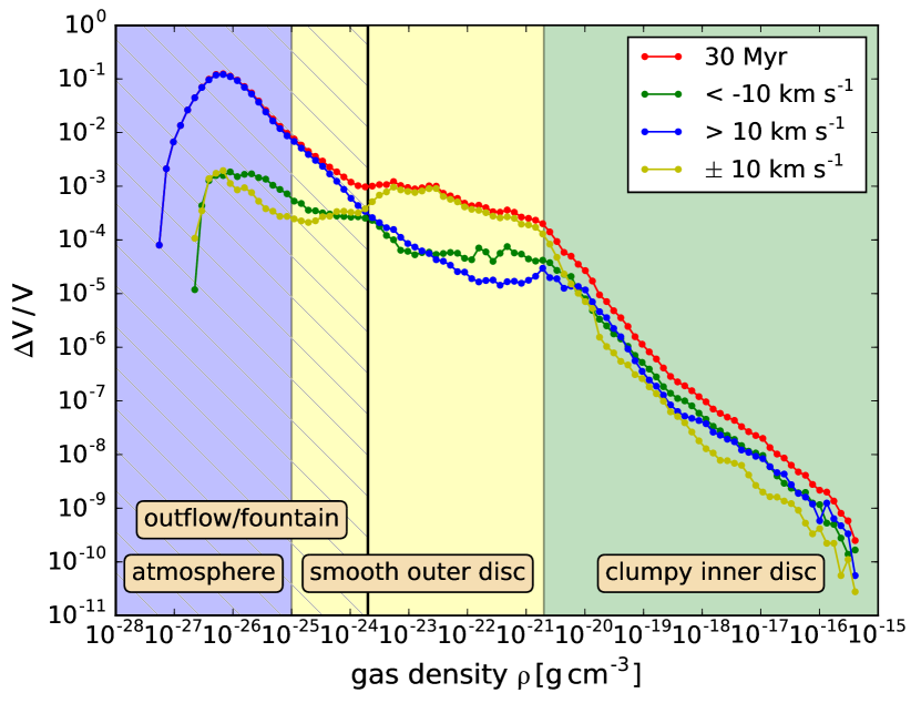
Figure 4: (a) Volume-weighted density probability distribution function (PDF) at several time snapshots as indicated in the legend, marking the initial condition (0 Myr), the clump formation epoch (5 Myr), the active outflow / fountain phase (30 Myr), the less active state (100 Myr) and the post-starburst, almost quiescent disc (250 Myr). (b) Density PDF at 30 Myr split into various radial velocity components as indicated in the legend. This permits clear separation of the smooth outer disc from the clumpy, star forming inner disc and the outflow / fountain flow. The volume for the plots is limited to a sphere with a radius of 512 pc surrounding the centre in order to remove the edges and outer regions of the cubic simulation box.

3.3 The mass budget, star formation and the stellar distribution

Fig. 5 shows the mass budget of the simulation. As soon as the gravitational instability enters the non-linear, clumpy phase, gas is efficiently turned into stars. Due to the strongly contracting clumps and high densities reached in the early evolution of the disc, the resulting SFR increases rapidly in the first 10 Myr, then reaches a maximum of roughly 1 M_⊙ yr^-1, followed by an exponential decrease (green stars in Fig. 10). The simulation leaves the starburst regime of the Kennicutt-Schmidt plane (within the red dotted lines in Fig. 11) after roughly 100 Myr. This is given by the dissolution of most of the clumps at that time. Such a relatively short starburst period is expected given the high gas densities, the short time scale of the fragmentation process and short gas depletion time in the nuclear region of our galaxy setup.

Concerning the stellar distribution, we will only discuss the distribution of the stellar particles, that were newly formed in the simulation in the following. It should be kept in mind that they spatially coexist with old stars from the stellar bulge. The latter – however – are taken into account as a background potential only. All of the stars form in dense clumps in our simulations. This is directly visible in the clumpy stellar surface density projected along the $z$-axis and $y$-axis during the starburst (see Fig. 6a,c). In the following evolution, a thick stellar disc is formed as the result of a relaxation process due to the interaction with the time-dependent local and global potential (Fig. 6b,d). Zooming onto and following the evolution of single stellar particles, we find that mergers of their host gas clump with minor gas concentrations offset the stellar particles from their originally centered position in the host gas clumps. This leads to the gradual heating of the stellar disc and the stars start orbiting the merger product. The strongest interactions occur during mergers of massive clumps, partly leading to a strong time dependence of the local potential and the ejection of the stellar particle from its host gas clump. Many additional encounters with massive clumps puff up and homogenise the stellar distribution to form a thick disc (Fig. 6b,d). The decreasing number density of clumps (and clump interactions) with time, substantially slows down relaxation, leading to long-lived stellar clumps at late stages of the simulation. One example is visible in the lower right quadrant of Fig. 6b.

The relaxation process is best visible in the azimuthally averaged stellar surface density distributions (projected along the z-axis) shown in Fig. 7, which also demonstrate that a converged distribution is reached after roughly 100-200 Myr. The process of thick stellar disc formation due to internal processes (clump-clump interactions) observed in our simulations is reminiscent of the formation of classical bulges (Noguchi, 1999; Immeli et al., 2004; Elmegreen et al., 2008) and exponential stellar discs (Bournaud et al., 2007) through clumpy disc evolution due to violent disc instabilities. This is found to be a very fast process that lasts only a few rotational periods (Elmegreen et al., 2008; Bournaud et al., 2009) consistent with our findings. Following different dynamics, a less violent process is the drift of the newly formed star clusters with respect to their parent clumps. This has been observed for the case of the Milky Way Galaxy, where relative drift velocities of around 10 km s^-1 have been found (Leisawitz et al., 1989).

Towards the end of the simulation time, the SFR and SN rate have decreased substantially and the system reaches an almost quiescent state again, in which the total mass budget is still (slightly) dominated by gas and only very low star formation and outflow rates are maintained. Only a small fraction of roughly 10% of the initial gas mass is lost in the tenuous, hot wind through the outer boundary of our simulation domain (yellow line in Fig. 5, assuming mass conservation of the code) corresponding to a total of roughly $9\times 10^{6}\,$M_⊙ within the 250 Myr computation time.

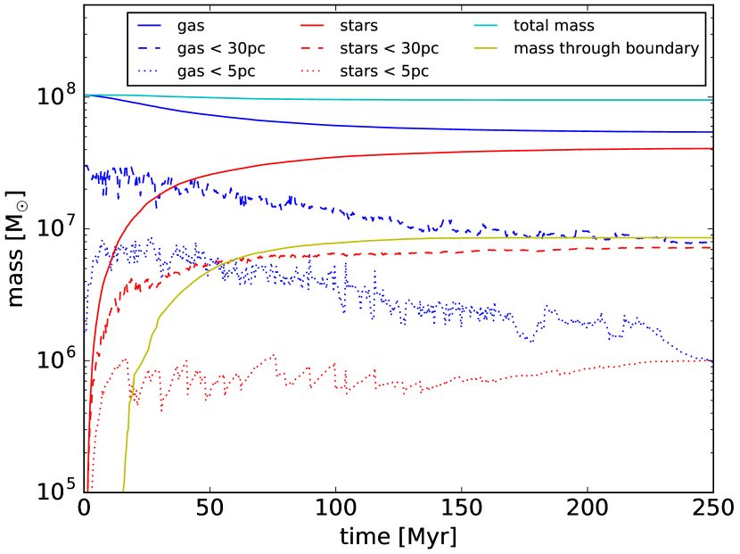
Figure 5: Evolution of the total mass in gas (blue) and stars (red) for the total domain (solid lines) and within a sphere of 30 pc (dashed lines) and 5 pc (dotted lines). The yellow line gives the cumulative mass lost through the boundaries of our simulation box. After the active phase of the starburst and a stable disc state has been reached, the total mass is still slightly dominated by gas.

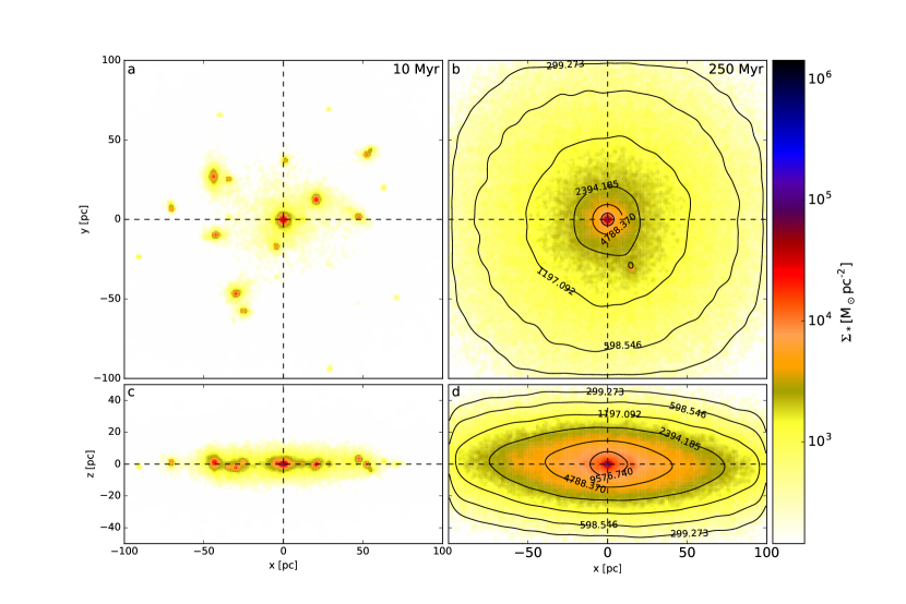
Figure 6: The stellar mass surface density projected along the $z$-axis (a,b) and $y$-axis (c,d) is shown, which has been derived on a grid with a bin size of 1 pc, smoothed with a Gaussian of FWHM=2 pc. Panels a and c depict the state during the early evolution of the starburst at 10 Myr and b and d in the almost quiescent, evolved state after 250 Myr. The black lines correspond to isodensity contours to better visualise the smooth, thick disc structure attained in the late time evolution. To derive the contours, the projected image has been smoothed with a Gaussian of FWHM=10 pc. Whereas the early evolution is characterised by an asymmetric distribution concentrated in a handful of clumps (corresponding to the birth places of the stellar particles), the stars settle into a thick disc-like, quasi-equilibrium structure, following relaxation mainly due to clump-clump interactions in the early, clumpy phase of the evolution.

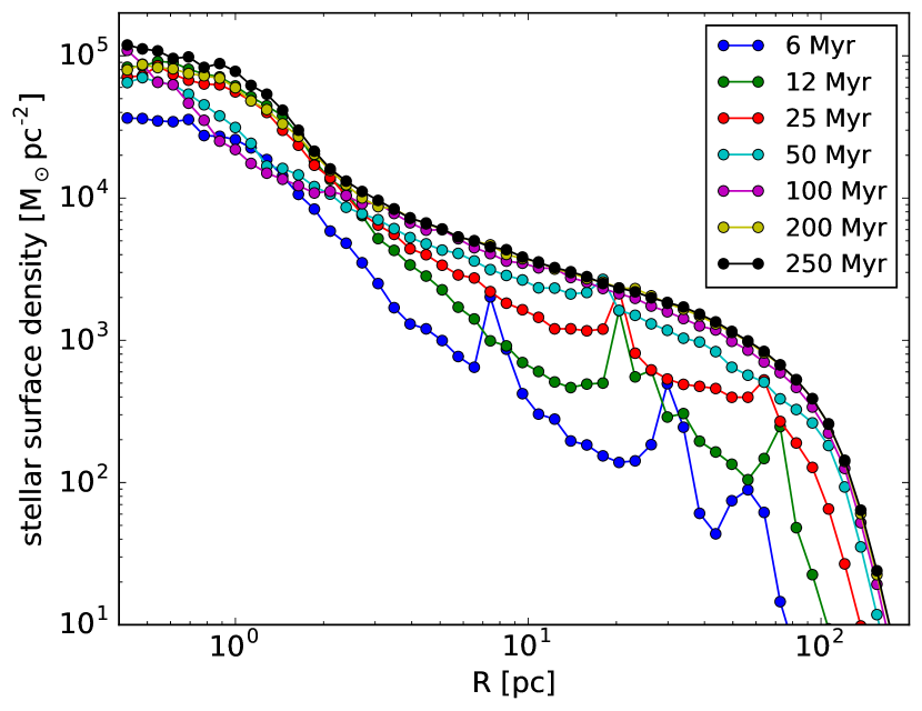
Figure 7: Projected radial stellar surface density profiles. The system relaxes from a distribution dominated by a small number of clumps to a converged, homogeneous, thick stellar disc.

3.4 Dynamical evolution of gas and stars

Fig. 8 shows the global mass weighted velocity dispersion of gas and stars in the direction perpendicular to the disc plane. The gas component is shown by the black line. The gas dispersion rises steeply during the first 10 Myr. As the gravitational instability produces clumps that carry a significant fraction of the total disc mass, they interact strongly, leading to a gravitational heating of the disc (see discussion in Sect. 3.3). To this end, the simulation without star formation (green line) shows a similar rising signature. Whereas the simulation without SF remains at roughly the same level (given by the relaxation of the gas clumps in the global potential and sustained by random motions of the clumpy medium with a low volume filling factor), the simulation with SF and SN feedback shows a decreasing trend of the gas dispersion. This is caused by the slow dissolution of the gas clumps caused by the ongoing star formation and feedback and the dissipative interaction with other clumps and the remaining smooth disc. The SN-driven fountain flow and outflow mostly affects the lower density gas and hence does not contribute substantially to the mass weighted velocity dispersion. With the dissolution of most of the clumps and the small remaining SN rate, the gas distribution settles into a thin disc configuration, resulting in a small value of the vertical gas velocity dispersion, slowly approaching the control run of a (low mass) Toomre stable disc (yellow line).

The stellar, vertical velocity dispersion (red line) shows a very similar behaviour to the gas dispersion in the no-SF case. Stars form mainly in the central regions of gas clumps within the equatorial plane of the disc, where the gas density is highest. Scattering events of stars with gas clumps – especially during clump merger events – lead to enhanced gravitational heating compared to the gas distribution. Finally, the stellar distribution relaxes in the global potential within roughly 30-40 Myr, leading to a constant velocity dispersion with time of roughly 40 km s^-1. This is slightly higher than the gas velocity dispersion in simulation no-SF in the second half of the simulation. We attribute the difference to the collisionless nature of the stellar particles, whereas the gaseous clumps dissipate energy in clump collisions and when moving through the smooth, ambient inter-clump gas.

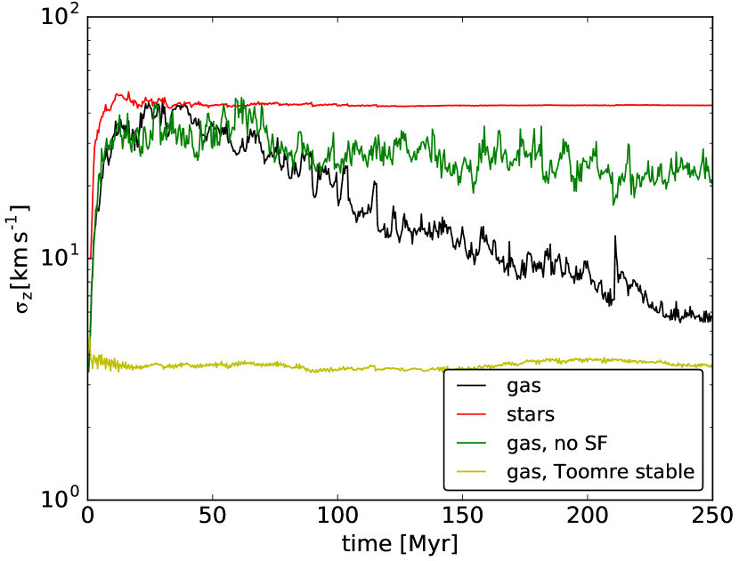
Figure 8: Global mass-weighted gas and stellar velocity dispersion in vertical direction. Clump-clump interactions during the early, non-linear stage of violent disc / Toomre instability transfer gravitational energy into random motions. The dissipationless evolution of the stellar particles enables a boost of the stellar heating process during clump-mergers (red line) compared to the clump-only simulation (green line, without star formation). The gas velocity dispersion of the simulation including star formation and feedback approaches the values of a Toomre stable (low mass) control simulation in the late stages of its evolution (yellow line).

3.5 Supernova feedback and starburst evolution

The global supernova rate is shown with blue symbols in Fig. 9. It can be roughly understood as the convolution of the global SFR (Fig. 10, green symbols) with the normalised SN delay time distribution (DTD; Fig. 2), which is shown as the yellow dashed line in Fig. 9. To this end, it shows a steep rise. The maximum is reached at around 30-40 Myr and – due to the convolution with the DTD – is delayed with respect to the one of the star formation history. The supernova rate (SNR) then follows an exponential decline until most of the dense enough gas has been used up for star formation and most of the massive stars have exploded as SN. Fig. 9 indicates that the supernovae in our simulation are strongly concentrated to the central region, which we show by restricting the calculated SNR to within spheres with certain radii (green and red circles). The concentration to the central region is expected due to the exponential profile of the initial gas distribution that only leads to a Toomre-unstable, central region of a few tens of parsecs (Fig. 1c). Viscous radial gas inflow during the evolution of the simulation further enhances this central concentration. The resulting supernova distribution follows the stellar distribution which evolves towards a double power-law radial profile with a central stellar density concentration (Fig. 7). The more we concentrate towards the nuclear region, the shallower the distribution and the stronger the fluctuations with time.

The fast relaxation of the stellar particles by clump-clump interactions allows many of them to leave their host clump and enables the formation of a stellar distribution with a moderately large scale height in vertical direction (Fig. 6). The subsequent SN explosions can then take place in a lower density environment, enabling higher efficiency to stir random motions and outflows. In contrast, most of the energy introduced due to SN in high density environments will be lost due to strong cooling, as the optically thin cooling applied in our simulations scales proportionally to the square of the gas density. Most of the early SN explosions will be located in the dense clumps and hence have only a small effect on the overall gas dynamics, whereas the progenitors of most of the later supernovae have already left their parent gas clump and are able to drive substantial random motions and outflows without major loss of energy via cooling radiation. The stellar relaxation and migration process hence changes the energy input mechanism substantially (see discussion in Sect. 3.6 and 5.3).

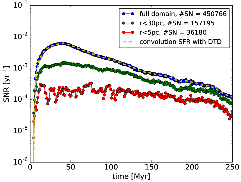
Figure 9: SN rates within the full domain and spheres of several radii as indicated in the legend. The global SN rate roughly follows the yellow dashed line, which depicts the convolution of the global star formation rate (SFR; Fig. 10, green stars) and the normalised supernova delay time distribution (DTD; Fig. 2).

3.6 Starburst-driven outflows and fountain flows

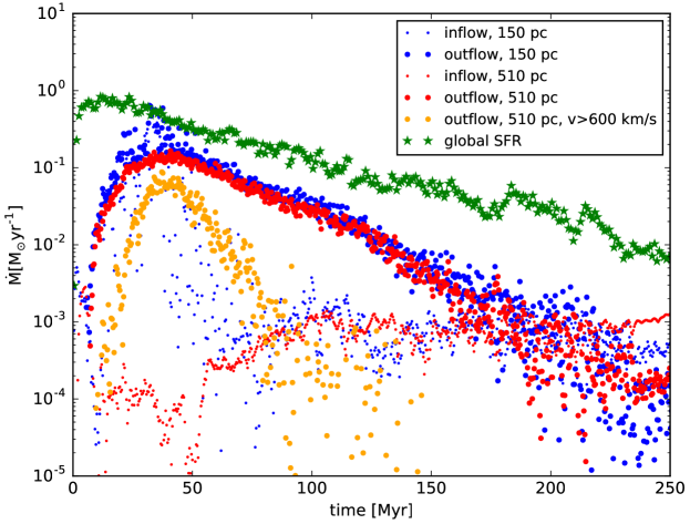
Figure 10: Global star formation rate and inflow / outflow through spherical shells at distances of 150 pc and 510 pc from the centre for the full evolution time of the simulation. The large-scale outflow (red thick circles) is directly correlated with the evolution of the SN rate (Fig. 9) during the most active phase of the starburst. The early evolution shows a fountain-like flow at small distances from the centre with similar in- and outflow rates (blue thin and thick circles) that turns into a strong outflow. Only during the peak of the starburst, a significant fraction of the outflow reaches escape velocity from the galaxy (orange symbols, for an assumed escape velocity of 600 km s^-1).

During the peak of the starburst, the strong energy input in supernova explosions drives both a low gas density outflow as well as a higher density fountain like flow (see Fig. 3). In order to quantify the two phenomena, we measure instantaneous gas in- and outflow rates from the simulation snapshots through two spherical shells at a radial distance from the centre of 150 and 510 pc with a thickness of $\Delta r=20$ pc:

$$\dot{M}=\frac{1}{\Delta r}\,\sum_{\mathrm{shell}}m_{\mathrm{i}}\,v_{\mathrm{i}}$$ (2)

where $m_{\mathrm{i}}$ and $v_{\mathrm{i}}$ are the mass and velocity of each cell within the spherical shell.

Fig. 10 shows the mass transfer rates calculated in this way as a function of time. This procedure allows us to quantify inflow (thin dots; radial velocity smaller than -10 km s^-1) as well as outflow (thick dots; radial velocity larger than 10 km s^-1) motion. The red symbols depict the measurements for the outer shell located at 510 pc distance from the centre. The outflow through this shell lags behind the star formation rate (green stars) and reaches its maximum after roughly 30-40 Myr following a shallower increase compared to the SFR. This delayed maximum of the outflow can again be explained by the DTD of the SNe and closely follows the SN rate with time with a slightly shallower increase towards the maximum, which we attribute to a combination of effects: (i) The efficiency of the energy input increases from the early SN explosions within dense clumps to SN explosions in the inter-clump medium due to stellar migration that heats the particle distribution by interaction with gas clumps. (ii) The high density fountain flow at low latitudes suppresses an outflow due to its relatively high gas column densities (see discussion in Sect. 5.1).

As the large-scale wind is driven from the central (initially Toomre-unstable) 50-100 pc region, the morphology resembles a cylindrical outflow during the most active phase (Fig. 3r,s). This is in contrast to radiatively-driven outflows from the central accretion disc which result in a more conical wind shape (e.g. Wada, 2012; Wada et al., 2016). Only around the peak of the starburst, a significant fraction of the outflow reaches escape velocity from the galaxy. This is shown by the orange symbols for an assumed escape velocity of 600 km s^-1. Looking at the shell close to the disc (blue symbols), the thin and thick symbols are close to one another for the first 40 Myr. This is mainly due to the fountain-like flow of the denser filaments that reaches beyond the shell position. These are part of the cold filaments visible in Fig. 3 around that time. After roughly 50 Myr – beyond the peak of the most active starburst – a steady outflow is formed with almost no back flowing filaments, even at the location of the inner shell. In- and outflow rates only become of similar strength after the starbursting phase at around 175 Myr.

4 Comparison to observations

4.1 Evolution in the Kennicutt-Schmidt diagram

Fig. 11 shows the evolution of the simulation in the plane given by the star formation rate surface density and the total gas surface density. To derive the data points, averages have been taken within a fixed (cylindrical) radius of 512 pc. This size ensures that all stars are included in the averaging process and the low density atmosphere within the simulation box is removed. Due to the short time scale of the structure and star formation process, both, the gas as well as the SFR surface densities increase rapidly until they approach the starburst Kennicutt-Schmidt (KS) relation (Daddi et al., 2010). The simulation starts at very high gas surface densities and first roughly follows the relation towards lower SFR surface density. This is by construction and used to calibrate our choice of the star formation efficiency. Then, the depletion of gas within the clumps due to star formation and stellar feedback processes results in a decrease of the average gas surface density. With the dissolution and merging of more and more clumps, the simulation starts deviating from the observed relation and leaves the starburst regime (within the red dotted lines) after roughly 75-100 Myr. After another approximately 50 Myr, most of the clumps have dissolved and only a handful of them remain in the central region. Observationally, gas depletion times have been found to be shorter in galactic centres compared to the rest of the galaxy (e. g.  Leroy et al., 2013). In the framework of our model, the duration of the starburst is a consequence of the marginally unstable initial condition, in which clumps are only formed in the central roughly 100 pc region of the gas disc and the short gas depletion time scale is equivalent to the starburst Kennicutt-Schmidt relation. Even shorter, Eddington-limited starbursts of the order of 10 Myr have been inferred from observations of circumnuclear discs of a sample of nearby Seyfert galaxies (Davies et al., 2007).

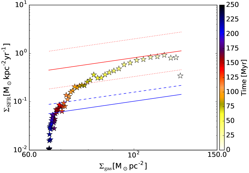
Figure 11: Evolution of the simulation in the Kennicutt-Schmidt diagram, colour-coded with the simulation time, averaged over 4 Myr. The quiescent KS relation derived by Daddi et al. (2010) is shown as the blue solid line whereas the red one refers to their starburst KS relation. The red dotted lines roughly give the observed scatter around the relation, the lower one roughly corresponding to the separation between bursting and quiescent star formation. The original KS relation (Kennicutt, 1998) is shown as the blue dashed line. Our simulation approaches the starburst KS relation from high gas surface densities, then evolves along the relation (by construction) and the depletion of the clumps leads to a deviation from the relation with time, before the SFR drops steeply after most of the clumps have dissolved.

4.2 Comparison to nuclei of nearby (active) galaxies

The gas mass within the central 30 pc region (corresponding to the scale length of the initial, exponential gas disc) is shown in Fig. 5 by the blue dashed line. It decreases slightly with time, reaching a value of around $10^{7}\,$M_⊙, in good correspondence to the observed Seyfert galaxy sample in Hicks et al. (2009). For the same sample, measurements of the velocity dispersions of the warm molecular hydrogen ($\approx$2000 K) via the 2.12 $\mu$m 1-0 S(1) line result in values of 50-100 km s^-1. For the cold gas phase represented by the 3mm HCN(1-0) line, lower velocity dispersions of 20-40 km s^-1 are derived (Sani et al., 2012). Lin et al. (2016) probe the velocity dispersion of the dense gas ($n_{\mathrm{H_{2}}}\approx 10^{4-5}\,\mathrm{cm}^{-3}$), resulting in a median velocity dispersion of $35$ km s^-1. These values for the cold, dense gas are compatible to our mass-weighted velocity dispersions shown in Fig. 8, which probe the high density component of the multi-phase gas in the simulations.

Using Keck/OSIRIS near-infrared (NIR) spectra, Durré & Mould (2014) investigate the circumnuclear disc in NGC 2110 (e. g.  Véron-Cetty & Véron, 2006; Rosario et al., 2010; Storchi-Bergmann et al., 1999) and find a total, nuclear star formation rate of $0.3\,$M${}_{\odot}\,\mathrm{yr}^{-1}$. This SFR is dominated by four massive and young star clusters that are embedded into a rotating nuclear disc of shocked gas in the inner 100 pc surrounding the active nucleus (see Fig. 2a, Durré & Mould, 2014). The shocked intercluster medium is thought to be excited by strong outflows that do not appear to originate from the AGN, but rather are localized to the clusters. This is reminiscent of the morphology of the stellar surface density in our simulations in the phase following Toomre instability and clump merging, that shows a handful of clumps orbiting in the nuclear potential in our simulations (e. g. Fig. 6a). These observed clusters could, therefore, be a sign of a recent event that triggered gravitational instability and the observed starburst and might have significant impact on the (ongoing and future) central activity (Davies et al., 2007).

The stellar distribution as well as kinematics of the central 10-150 pc in active and inactive galactic nuclei within the LLAMA (Luminous Local AGN with Matched Analogues, Davies et al., 2015) sample has been analysed by M. -Y. Lin et al. (2017, submitted). After subtraction of the underlying stellar bulge distribution, a stellar light excess is found in most of the sources, which amounts to a few percent of the stellar mass of the underlying bulge within the central 3 arcseconds. This excess emission is found to be consistent with rotating stellar nuclear discs, which follow a size-luminosity relation in which the size of the stellar system is roughly proportional to the square root of the stellar luminosity. For the final snapshot of our simulation at 250 Myr, we find that 99% of the stellar mass is inside a radius of 173 pc. Assuming a mass-to-light ratio of 1.5 for this relatively young stellar population (see Fig. 4c in Davies et al., 2007) results in a total luminosity of $3\times 10^{7}\,$L_⊙. This places the final state of our simulation very close to the observed relation. During the early evolution, the simulation is located above the relation (but already within the observed scatter after a few Myrs), and approaches it with time.

On top of the large scale stellar disc, a second component is found in the central few parsec regime (Fig. 7). The latter is characterised by fitting a Sérsic profile up to a distance of 2 pc. We find a Sérsic index of 0.6, an effective radius of 1.2 pc and a total mass of roughly $8\times 10^{5}$ M_⊙ after 250 Myr of evolution. This is reminiscent of nuclear star clusters (NSC) that are frequently observed in the centres of galaxies of all Hubble types. Their observed dynamical masses are in the range of $10^{4}$ to $10^{8}$ M_⊙ with effective radii between $0.1-100$ pc (e. g.  Balcells et al., 2007; Kormendy et al., 2010; Georgiev et al., 2016). Our simulated NSC is within the scatter of the mass-size relation the latter authors find, located rather at the lower mass and size end of the distribution. The star formation histories are observationally found to be rather long and quite complex and seem to require multiple epochs of recurrent star formation (Neumayer, 2012). Together with the finding of NSC rotation as a whole (Seth et al., 2008, 2010), these observed characteristics nicely match the stellar system found in our simulation, which might correspond to the first star formation epoch. Subsequent disc instabilities (following additional mass inflow from the galaxy) might lead to a growth in mass and size. However, it should be kept in mind that at these distances from the centre we are within the smoothing scale of the central SMBH potential, which makes further investigations necessary.

With the advent of the ALMA observatory, more and more high spatial and spectral resolution data on nearby AGN becomes available. A particularly interesting case is the Circinus galaxy, the nearest Seyfert 2 galaxy. The molecular gas in its central 1 kpc region has been studied in great detail in CO (1-0) line emission by Zschaechner et al. (2016). They find evidence for a molecular component in the well-established ionised gas outflow with an outflow rate of 0.35 to 12.3 M_⊙, which is comparable to its (global) star formation rate of 4.7 M_⊙ yr^-1 (For et al., 2012). This is regarded as an indication that the outflow regulates the SF. A velocity dispersion of 30-50 km s^-1 has been found in the central roughly 5 arcsec and 30-40 km s^-1 in the outflow. A total molecular mass of the disc within 1.5 kpc of 2.9$\times 10^{8}$ M_⊙ has been inferred. All of these numbers – as well as the hint for a filamentary structure in the wind – are roughly compatible to what we find in our simulations during the actively starbursting episode. However, in our simulations, the star formation regulates the outflow and not vice-versa and the outflow rates are close to the lower limit of the observationally derived outflow rate, allowing for additional outflow driven by the active nucleus.

IC 630 is a nearby early-type galaxy, classified as a radio galaxy (Brown et al., 2011). With the help of VLT-SINFONI and Gemini North-NIFS adaptive optics observations, Durré et al. (2017) show that the excitation of the circumnuclear gas within a few 100 pc of the centre can mostly be explained by star formation. The measured SFR (1-2 M_⊙ yr^-1), SNR ($4\times 10^{-3}$ yr^-1), the gas outflow rate (0.18 M_⊙ yr^-1), total gas masses (a few times $10^{7}$ M_⊙) as well as the line of sight velocity channel maps of the gas all are in line (within a factor of a few) with our simulated system during the peak of the starbursting phase, seen face-on. Especially the inferred young starburst age of roughly 6 Myr (derived from the equivalent width of the Brackett-$\gamma$ line) and the observed cylindrical rather than conical shape of the outflow points into a starburst-, rather than AGN-driven event. Also the clumpy structure in the observed NIR J, H and K band maps as well as the hint of a spiral structure is in good agreement with the structural evolution found from our violent disc instability scenario.

Overall, we find good agreement with available observations, indicating that the physical scenario investigated in this paper could be at work in several nearby (active) galactic nuclei.

5 Discussion

5.1 Obscuring properties

Fig. 12 shows the obscured fraction as a function of time for the gas distribution of our simulation. For each data point, we calculate 1000 rays from the centre to determine the hydrogen column density. Shown is the resulting obscured fraction defined as the fraction of these rays having a hydrogen column density in excess of $10^{22}\,\mathrm{cm}^{-2}$ (blue circles) and $10^{24}\,\mathrm{cm}^{-2}$ (green stars). Due to resolution limitations we are currently not able to resolve AGN tori or nuclear maser emitting discs. In the nearby active galaxies we are concentrating on, the latter are expected to have sizes in the sub-pc to pc regime (e. g.  Greenhill et al., 1996; Greenhill et al., 2003; Burtscher et al., 2013; Tristram et al., 2014; García-Burillo et al., 2016). To this end, we exemplify the obscured fractions by removing the central $5\,$pc, concentrating on the starburst-driven flow. Under these conditions, we find that during the starburst, the stirred-up gas as well as the randomised clump dynamics – mainly in the tens of parsecs distance regime – can make a significant contribution to the overall obscured fraction. This can be seen by comparing to the observationally derived obscured fractions, which are shown by the horizontal dotted and dashed lines in the corresponding colours, which have been adapted from Buchner et al. (2015) and Ricci et al. (2015), respectively. However, it should be kept in mind that the central cut-out region contains a significant amount of mass (see Fig. 5, blue dotted line and Sect. 5.2). Changing the radius of the inner cut-out region shifts the curves in vertical direction.

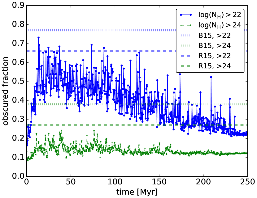
Figure 12: Obscured fraction as a function of time for log(N_H[cm^-2])>22 (circles and blue solid lines) and log(N_H[cm^-2])>24 (stars and green dashed lines). The inner region has been cut out up to a radius of 5 pc. Shown as well are the values derived from observations by Buchner et al. (2015) (B15) and Ricci et al. (2015) (R15). This shows that a nuclear starburst on tens to hundreds of parsec scale is able to significantly contribute to the obscured fraction and leads to a time varying additional obscuration.

5.2 Effects on AGN tori

AGN tori are expected to be located within the central few parsecs region (Jaffe et al., 2004; Burtscher et al., 2013; Tristram et al., 2014; García-Burillo et al., 2016; Gallimore et al., 2016). In our simulations, a very dynamic picture emerges in this radius regime: spiral patterns build up as a consequence of Toomre instability in the first few Myr of the evolution until they break up into clumps. Merging together, they form a dense disc structure around the central 2-3 pc region, which actively forms stars and is often affected by mergers with clumps and tidal arms. After most of the clumps have dissolved (at an evolution time of roughly 230 Myr), a tightly-wound spiral density enhancement remains around the central disc-component, which slowly decreases in density due to the formation of stars. Additionally taking this distance regime into account in the calculation of the obscured fraction of our simulation (see Sect. 5.1), we find a larger scatter compared to the case excluding the central 5 pc and the values reach obscured fractions of 1 for the low column density lines of sight for a significant fraction of the time. An enhanced time variation is also found after integrating the total gas mass within the central 5 pc sphere (blue dotted line in Fig. 5). As this time variation is caused by clumps merging into the central (gas and stellar) density concentration, this indicates that the clumpy circumnuclear disc evolution might have a significant influence on the dynamics and morphology of AGN tori, as well as BH feeding properties on these variation time scale. This might be a further indication that tori are time-dependent or even transient structures, rather than showing long-term stability during such active phases of nuclear star formation. The disturbances caused by inspiraling clumps might as well cause perturbations of the central disc/torus and form warped discs that are often observed in nearby Seyfert nuclei due to their maser emission (e. g.  Greenhill et al., 1996; Greenhill & Gwinn, 1997; Greenhill et al., 2003). Central warped discs have been found to significantly change the mid-IR characteristics (Jud et al., 2017) as well as partly influence the polarisation signal (F. Marin & M. Schartmann, 2017, submitted) of the nuclear gas and dust distribution. Infalling clumps (or fragments thereof) merging into the central discs might cause significant gravitational heating (Klessen & Hennebelle, 2010), leading to phases of geometrically thick discs or tori and might trigger short-duration, nuclear activity cycles. Significant impact on the IR emission due to these morphological transformations on parsec scale can be expected, resulting in a diversity of AGN tori, as e. g. seen in a sample of nearby Seyfert galaxies, observed with the MIDI instrument (Burtscher et al., 2013). Our current spatial resolution is not high enough to test this hypothesis and the results should be regarded as tentative, but this should be feasible in near-future simulations.

5.3 Comparison to published simulations

Wada et al. (2009) have investigated models of starbursting circumnuclear discs, targeted at nearby Seyfert galaxies. Starting with an initially constant surface density disc, they find that a gas distribution in (approximate) equilibrium is obtained within less than 5 Myr. This consists of a puffed-up toroidal structure on tens of parsecs scale that surrounds a geometrically thin disc on several parsec scale. SN feedback in the latter drives a low density, hot outflow with a velocity of several 100 km s^-1. They assumed a range of SN rates between $5-500\times 10^{-5}\,\mathrm{yr}^{-1}$ (within a radius of 26 pc and a height of 2 pc). Restricting the analysis of our simulations to the central 30 pc region, we find rates of around $10^{-3}$ SN per year over a time frame of roughly 150 Myr (green line in Fig. 9). This is close to their upper limit. The main difference between the simulations is the distribution of gas, which is concentrated to the central region in our exponential surface density distribution. Self-consistently following the stellar dynamical evolution, we find that the star particles are also very centrally concentrated (Fig. 6, right column and Fig. 7) in the evolved state of our simulations. Consequently, the SN distribution is much more centrally concentrated compared to a spatially random distribution within a thin disc as was used in Wada et al. (2009). Reaching out to much larger scale heights in our resulting thick stellar disc configuration, our model shows more SN explosions in lower density regions off the midplane of the disc. The latter are more effective in driving stronger outflows and fountain flow behaviour, compared to the toroidal structure found in Wada et al. (2009).

Overall, the driving of random motions and outflows due to supernova explosions in our simulations can be regarded as a mixture between what has been dubbed as peak driving (explosions happen in high density clumps) and random driving (where the SN are randomly distributed within the computational domain) in idealised simulations (Gatto et al., 2015; Walch et al., 2015). Stars in our simulations (as well as in nature) form in dense gas clumps. Depending on the delay time distribution, a fraction of the SN explosions happen at these locations of very high gas densities (peak driving). These correspond mostly to the high mass progenitor stars and to clumps that have suffered very little scattering and merging processes with other clumps. Due to the short cooling time, mostly small bubbles are formed that have only little effect on the evolution of the clump and are barely able to drive significant outflows from the central region. The stellar relaxation through the interaction of clumps allows the SN progenitor stars to leave the high density regions and explode in a lower density environment. This changes the mechanism to distributed or mixed driving, which results in a more efficient coupling of the SN input energy to the low density gas, producing and sustaining an outflow perpendicular to the disc plane. This clearly shows the necessity of (i) a self-consistent treatment of the dynamical evolution of the stellar distribution as well as (ii) the implementation of a delay time distribution for the SN explosions.

The role of inflows for the cyclic appearance of nuclear starbursts has been investigated by a number of publications. In a global, very high-resolution simulation of a Milky Way-like galactic disc, Emsellem et al. (2015) study the self-consistent formation of a stellar bar that regulates the mass transfer towards the central kiloparsec region. Accumulating in ring-like distributions at Lindblad resonances, the gas is able to form stars at the edge of the bar only. Stellar feedback interaction allows further gas feeding towards the centre within a minispiral. Shear inside the bar region inhibits star formation, allowing the transfer of gas through the minispiral and the formation of a disc at around 10 pc distance from the centre, in which clumps form that partly disrupt into long filaments due to the tidal interaction with the SMBH or form a nuclear star cluster. Many similarities are found between the gas and stellar distribution compared to the Galactic Centre of the Milky Way. Compared to our circumnuclear disc in isolation, this simulation including the feeding from larger scales shows a similar behaviour. Whenever gas is able to accumulate, stars are formed, which confirms the importance of gravitational instability for the formation of structure in the circumnuclear environment. The Milky Way simulation shows the case of a low mass inflow rate that leads to rather low mass concentrations and episodic star formation on short time scale in this very inactive galactic nucleus. Our massive gas disc must have either accumulated over a longer time period or must have been formed by a high mass inflow rate in order to cause a much stronger starburst and fast, hot outflowing gas.

Concentrating on the central 500 pc region of the Milky Way (the so-called Central Molecular Zone, CMZ), a self-consistent model for star formation cycles based on theoretical arguments and observed properties has been developed by Kruijssen et al. (2014). Within a galaxy-scale gas inflow (e. g. bar-driven), acoustic and gravitational instabilities concentrate the gas until a star formation density threshold is reached. The latter might be environmentally dependent and increased in galactic nuclei due to enhanced levels of turbulence, which is consistent with the assumptions of our simulations. Their model allows to explain the currently low star formation rate (SFR) in the CMZ. It seems to be in the slow phase of accumulating gas that limits the rate of star formation. This will be followed by rapid gas consumption into stars, once the density threshold for gravitational instability is reached. Our simulations assume an initial condition that is comparable to the end of the accumulation stage of the model found by Kruijssen et al. (2014) and gravitational instability is able to occur. Given the higher accumulated mass, a more intense and a longer starburst follows compared to what is found for the Milky Way. This is the phase we concentrate on in this publication and resolve in great detail in space as well as time. After roughly 250 Myr, our disc returns into the accumulation phase again with a star formation rate below what is expected from the Kennicutt-Schmidt relation (see Fig. 11). Hence our initial condition and the expected cyclic behaviour is consistent with models including the feeding of gas from larger scales.

5.4 Numerical issues and resolution dependence

The simulation of circumnuclear discs with sub-parsec resolution is especially demanding, as they are located deep within the gravitational potential well of the stellar bulge and SMBH and have very high density contrasts. This not only necessitates very high spatial resolution, but the corresponding dynamics and short cooling timescales require very short timesteps, making the simulations very computationally expensive. As we are interested in simulating full activity cycles, long time evolutions of several tens of revolutions of the disc are necessary. Another reason for high resolution is to avoid artificial fragmentation of the self-gravitating gas. To this end, we require that the Jeans length is resolved with at least 4 grid cells, following (Truelove et al., 1997). This is achieved first of all by triggering refinement when the Jeans length is not resolved well enough (see Sect. 2.2). To fulfill the Truelove-criterion even at the highest refinement level, the usual artificial pressure floor is used (Sect. 2.6). This only affects the highest densities within the clumpy structures. The consequence of using a density threshold for star formation as large as $2\times 10^{6}\,\mathrm{cm}^{-3}$ is that for our given maximum resolution, a fraction of the star formation happens within cells that are heated to $10^{4}-10^{5}$ K. However, these cells are deeply embedded into the high density gas clumps.

We generally find good convergence of the simulation when increasing the resolution by halving the refinement threshold masses by factors of two. The same is true for a simulation with double the stellar particle mass, e. g. converging to the same stellar velocity dispersion, with differences only arising in the early relaxation phase.

Using a Cartesian grid, the code conserves linear momentum only. The high resolution in the fragmenting part of the disc guarantees a reasonable angular momentum conservation (within 10%) in this region of the computational box. In this publication, we are not interested in the evolution of the smooth outer disc. Including the latter in the angular momentum balance, we find deviations from the initial value of up to 50% at the end of the simulation, which corresponds to roughly 45 orbits at a radius of 150 pc. This is evident in the evolution of the surface density in the outer part of the radial range shown in Fig. 1b as well as the changing size of the outer disc (Fig. 3a-d).

5.5 Limited physics

Our simulations start with an (isolated) Toomre unstable, self-gravitating, high density gas disc in approximate vertical hydrostatic equilibrium. We show that such an initial configuration allows recovery of many observed properties of nearby circumnuclear discs during the evolution of the simulation. Resulting disc masses (gas and stars), the kinematical state, star formation properties and the subsequent driving of a wind are in reasonable agreement with observed properties. However, the question remains how such a disc can be build up and stabilised against collapse. Gas at such high densities cools on a very short time scale. Allowing the cooling down to molecular cloud core temperatures would lead to a collapse to a thin (unresolvable) disc within an orbital time scale in our simulations. Numerically, we prevent this by setting a minimum temperature of $10^{4}$ K, which is thought to replace unresolvable micro-turbulence, corresponding to a velocity dispersion of the order of $10\,$km s^-1 as well as photoionisation heating once a young stellar population has been formed. As the Toomre stability criterion depends on the gas temperature and kinematical state of the gas, this assumption has an important effect on the gravitational stability and allows investigation of well-defined initial conditions. In reality nuclear regions are not isolated from larger galactic features, but gas is dynamically driven inwards through bars, spirals, etc. Plunging into the central disc, this accreted gas releases part of its kinetic energy and leads to turbulent gas motions within the disc. The strength of this effect depends on the amount of gas present, the mass infall rate and velocity, the turbulent driving scale as well as an efficiency factor. Balancing the energy input with the turbulent dissipation rate, Klessen & Hennebelle (2010) find

$$\dot{M}_{\mathrm{in}}=0.39\,\mathrm{M}_{\odot}\,\mathrm{yr}^{-1}\,\left(\frac{0.1}{\epsilon}\right)\,\left(\frac{M_{\mathrm{gas}}}{10^{8}\,\mathrm{M}_{\odot}}\right)\,\left(\frac{\sigma}{10\,\mathrm{km}\,\mathrm{s}^{-1}}\right)^{3}\,$$ (3)

$$\left(\frac{100\,\mathrm{pc}}{L_{\mathrm{d}}}\right)\,\left(\frac{160\,\mathrm{km}\,\mathrm{s}^{-1}}{v_{\mathrm{in}}}\right)^{2}.$$ (4)

Using the gas disc mass of our initial condition (M${}_{\mathrm{gas}}=10^{8}$ M_⊙), a gas infall velocity similar to the rotation velocity ($v_{\mathrm{in}}=160$ km s^-1), a turbulent driving scale similar to the thickness of the gas disc ($L_{\mathrm{d}}=100$ pc) and a typical efficiency of $\epsilon=10$% (Klessen & Hennebelle, 2010), the process requires a mass infall rate of the order of 0.39 M_⊙ yr^-1 to reach a velocity dispersion of roughly $\sigma=10\,\mathrm{km}\,\mathrm{s}^{-1}$. Following these simple energy arguments, the resulting mass infall rates are in the range of observed infall rates of 0.01-1 M${}_{\odot}\,\mathrm{yr}^{-1}$ in nearby Seyfert galaxies (e. g.  Storchi-Bergmann, 2014). This simplistic analysis also shows that the more mass is accumulated by infall and the closer we get to our high mass initial state, the more difficult it is to maintain the necessary turbulent motions. As the reasoning is based on simple energy arguments, high resolution simulations including the feeding from larger scales are needed in order to test this hypothesis. This will also lead to replenishment of the gas compared to our current closed-box model, allowing either prolongation of the star formation episode or initiation of subsequent star formation episodes. Whether such a small-scale turbulent pressure floor is equivalent to a thermal pressure is a question on its own.

Only limited physical mechanisms are applied in our implementation of stellar feedback. We idealise it in a single event, which we denominate as a supernova explosion. Each event introduces an energy of $10^{51}$ erg into the surrounding medium. In reality, massive stars interact with their environment in multiple ways. They drive winds of various strengths and morphologies and ionise their surrounding interstellar medium. Even the supernova explosions themselves show a variety of energies. To this end, the feedback modelling we use in this first set of simulations should be regarded as an effective total energy input, summarising the mentioned effects, that contribute to the scatter around this energy input and add to its uncertainty. Future modelling efforts should allow to determine the main effects and to concentrate on the small scale differences.

The clump dynamics and stellar feedback enhance the effective viscosity of the disc and drive gas inwards. According to its angular momentum, the gas will finally end up in the accretion disc / torus system and – after a not very well known time delay depending on the effective viscosity – will lead to the activation of the central nuclear activity. In this paper we concentrate on the effect of stellar feedback alone. Nuclear activity mainly impacts the central region of the circumnuclear disc, possibly driving a high velocity outflow, including some back flow that drives turbulent motions and might lead to the formation of high column density toroidal structures (e. g.  Wada, 2012, 2015).

6 Conclusions

Using high-resolution hydrodynamical simulations with the Ramses code (Teyssier, 2002) we investigate the interstellar medium in initially marginally stable self-gravitating circumnuclear discs in galactic nuclei. We follow the gravitational collapse, the non-linear growth of structure and the subsequent nuclear starburst phase self-consistently, including the gravitational potential of a central SMBH and a galactic bulge (following scaling relations), the self-gravity of the gas disc, standard optically thin cooling and a model SN delay time distribution. First, concentric rings and spiral-like features form due to Toomre instability that – during the non-linear evolution of the instability – break up into clumps which are able to form stars. Clump-clump merging as well as scatterings lead to the formation of a thick gas and stellar disc. During the peak of the nuclear starbursting phase, we find that the gas forms a three component structure: (i) An inhomogeneous, high density, clumpy and turbulent cold disc is puffed-up due to an increase in vertical velocity dispersion caused by clump-clump interactions and should be observable with ALMA. (ii) It is surrounded by a geometrically thick distribution of dense clouds and filaments above and below the disc midplane which form a fountain-like flow, visible in the infrared IFU data. (iii) And a tenuous, hot, ionised outflow (visible in HST imaging data) leaves the disc perpendicular to its midplane. The star formation decreases as a larger and larger fraction of the high density gas clumps are used up by star formation and have partly expelled their gas by stellar feedback processes. For the initially marginally stable gas disc around a low mass black hole ($10^{7}\,$M_⊙) and bulge ($9\times 10^{9}\,$M_⊙) under investigation, the active starbursting phase takes of the order of 150-200 Myr after which it turns into an almost quiescent disc with a low star formation and outflow rate. Starting from initial and boundary conditions that are guided by observed properties of nearby active galactic nuclei, we find good correspondence of many of the simulated stages of evolution with observed quantities. A handful of star forming clumps are frequently found in observations of nearby circumnuclear discs. The nuclear disc masses, star formation rates, supernova rates as well as wind mass loss rates derived from integral field unit observations are in reasonable agreement with the findings of our simulated galactic nucleus. In order to achieve this, it is necessary to follow the formation of the stars and their subsequent dynamical relaxation process self-consistently and model a delay time distribution of the SN feedback, to allow a fraction of the stars to leave their parent high density clump. Another result of this evolution is a disc of young stars (with a tentative central nuclear star cluster component) that fits the recently found size-luminosity relation for such nuclear stellar discs as well as their observed kinematical state. The combination of such simulations with the large amount of high resolution, multi-wavelength, multi-instrument observational data that will be available in the coming years will test the scenario described above and will allow us to build a consistent picture of inflow, excitation, SF and outflow of the circumnuclear gas.

References

- Agertz et al. (2009) Agertz O., Teyssier R., Moore B., 2009, MNRAS, 397, L64
- Antonucci (1993) Antonucci R., 1993, ARA&A, 31, 473
- Balcells et al. (2007) Balcells M., Graham A. W., Peletier R. F., 2007, ApJ, 665, 1084
- Barnes (2002) Barnes J. E., 2002, MNRAS, 333, 481
- Behrendt et al. (2015) Behrendt M., Burkert A., Schartmann M., 2015, MNRAS, 448, 1007
- Behrendt et al. (2016) Behrendt M., Burkert A., Schartmann M., 2016, ApJ, 819, L2
- Berg et al. (2014) Berg T. A. M., Simard L., Mendel Trevor J., Ellison S. L., 2014, MNRAS, 440, L66
- Bournaud et al. (2007) Bournaud F., Elmegreen B. G., Elmegreen D. M., 2007, ApJ, 670, 237
- Bournaud et al. (2009) Bournaud F., Elmegreen B. G., Martig M., 2009, ApJ, 707, L1
- Brown et al. (2011) Brown M. J. I., Jannuzi B. T., Floyd D. J. E., Mould J. R., 2011, ApJ, 731, L41
- Buchner et al. (2015) Buchner J., et al., 2015, ApJ, 802, 89
- Burtscher et al. (2013) Burtscher L., et al., 2013, A&A, 558, A149
- Chapon et al. (2013) Chapon D., Mayer L., Teyssier R., 2013, MNRAS, 429, 3114
- Daddi et al. (2010) Daddi E., et al., 2010, ApJ, 714, L118
- Dalgarno & McCray (1972) Dalgarno A., McCray R. A., 1972, ARA&A, 10, 375
- Davies et al. (2007) Davies R. I., Mueller Sánchez F., Genzel R., Tacconi L. J., Hicks E. K. S., Friedrich S., Sternberg A., 2007, ApJ, 671, 1388
- Davies et al. (2014) Davies R. I., et al., 2014, ApJ, 792, 101
- Davies et al. (2015) Davies R. I., et al., 2015, ApJ, 806, 127
- Downes & Solomon (1998) Downes D., Solomon P. M., 1998, ApJ, 507, 615
- Dubois & Teyssier (2008) Dubois Y., Teyssier R., 2008, A&A, 477, 79
- Durré & Mould (2014) Durré M., Mould J., 2014, ApJ, 784, 79
- Durré et al. (2017) Durré M., Mould J., Schartmann M., Ashraf Uddin S., Cotter G., 2017, ApJ, 838, 102
- Elmegreen (2011) Elmegreen B. G., 2011, ApJ, 731, 61
- Elmegreen et al. (2008) Elmegreen B. G., Bournaud F., Elmegreen D. M., 2008, ApJ, 688, 67
- Emsellem et al. (2015) Emsellem E., Renaud F., Bournaud F., Elmegreen B., Combes F., Gabor J. M., 2015, MNRAS, 446, 2468
- Federrath et al. (2008) Federrath C., Klessen R. S., Schmidt W., 2008, ApJ, 688, L79
- Ferland et al. (1998) Ferland G. J., Korista K. T., Verner D. A., Ferguson J. W., Kingdon J. B., Verner E. M., 1998, PASP, 110, 761
- Fierlinger et al. (2016) Fierlinger K. M., Burkert A., Ntormousi E., Fierlinger P., Schartmann M., Ballone A., Krause M. G. H., Diehl R., 2016, MNRAS, 456, 710
- For et al. (2012) For B.-Q., Koribalski B. S., Jarrett T. H., 2012, MNRAS, 425, 1934
- Fukuda et al. (2000) Fukuda H., Habe A., Wada K., 2000, ApJ, 529, 109
- Gallimore et al. (2016) Gallimore J. F., et al., 2016, ApJ, 829, L7
- García-Burillo et al. (2016) García-Burillo S., et al., 2016, ApJ, 823, L12
- Gatto et al. (2015) Gatto A., et al., 2015, MNRAS, 449, 1057
- Georgiev et al. (2016) Georgiev I. Y., Böker T., Leigh N., Lützgendorf N., Neumayer N., 2016, MNRAS, 457, 2122
- Greenhill & Gwinn (1997) Greenhill L. J., Gwinn C. R., 1997, Ap&SS, 248, 261
- Greenhill et al. (1996) Greenhill L. J., Gwinn C. R., Antonucci R., Barvainis R., 1996, ApJ, 472, L21+
- Greenhill et al. (2003) Greenhill L. J., et al., 2003, ApJ, 590, 162
- Häring & Rix (2004) Häring N., Rix H.-W., 2004, ApJ, 604, L89
- Harten et al. (1983) Harten A., Lax P. D., van Leer B., 1983, SIAM REVIEW, 25, 35
- Hernquist (1990) Hernquist L., 1990, ApJ, 356, 359
- Hicks et al. (2009) Hicks E. K. S., Davies R. I., Malkan M. A., Genzel R., Tacconi L. J., Müller Sánchez F., Sternberg A., 2009, ApJ, 696, 448
- Hicks et al. (2013) Hicks E. K. S., Davies R. I., Maciejewski W., Emsellem E., Malkan M. A., Dumas G., Müller-Sánchez F., Rivers A., 2013, ApJ, 768, 107
- Hönig et al. (2006) Hönig S. F., Beckert T., Ohnaka K., Weigelt G., 2006, A&A, 452, 459
- Hopkins & Quataert (2010) Hopkins P. F., Quataert E., 2010, MNRAS, 407, 1529
- Immeli et al. (2004) Immeli A., Samland M., Gerhard O., Westera P., 2004, A&A, 413, 547
- Jaffe et al. (2004) Jaffe W., et al., 2004, Nature, 429, 47
- Jud et al. (2017) Jud H., Schartmann M., Mould J., Burtscher L., Tristram K. R. W., 2017, MNRAS, 465, 248
- Kennicutt (1998) Kennicutt Jr. R. C., 1998, ApJ, 498, 541
- Klessen & Hennebelle (2010) Klessen R. S., Hennebelle P., 2010, A&A, 520, A17
- Kormendy et al. (2010) Kormendy J., Drory N., Bender R., Cornell M. E., 2010, ApJ, 723, 54
- Krolik & Begelman (1988) Krolik J. H., Begelman M. C., 1988, ApJ, 329, 702
- Kruijssen et al. (2014) Kruijssen J. M. D., Longmore S. N., Elmegreen B. G., Murray N., Bally J., Testi L., Kennicutt R. C., 2014, MNRAS, 440, 3370
- Krumholz & Kruijssen (2015) Krumholz M. R., Kruijssen J. M. D., 2015, MNRAS, 453, 739
- Krumholz & McKee (2005) Krumholz M. R., McKee C. F., 2005, ApJ, 630, 250
- Krumholz & Tan (2007) Krumholz M. R., Tan J. C., 2007, ApJ, 654, 304
- Krumholz et al. (2012) Krumholz M. R., Dekel A., McKee C. F., 2012, ApJ, 745, 69
- Leisawitz et al. (1989) Leisawitz D., Bash F. N., Thaddeus P., 1989, ApJS, 70, 731
- Leitherer et al. (1999) Leitherer C., et al., 1999, ApJS, 123, 3
- Leitherer et al. (2014) Leitherer C., Ekström S., Meynet G., Schaerer D., Agienko K. B., Levesque E. M., 2014, ApJS, 212, 14
- Leroy et al. (2013) Leroy A. K., et al., 2013, AJ, 146, 19
- Levine et al. (2008) Levine R., Gnedin N. Y., Hamilton A. J. S., Kravtsov A. V., 2008, ApJ, 678, 154
- Lin et al. (2016) Lin M.-Y., et al., 2016, MNRAS, 458, 1375
- Lupi et al. (2015) Lupi A., Haardt F., Dotti M., Colpi M., 2015, MNRAS, 453, 3437
- Machacek et al. (2001) Machacek M. E., Bryan G. L., Abel T., 2001, ApJ, 548, 509
- Maciejewski (2004a) Maciejewski W., 2004a, MNRAS, 354, 883
- Maciejewski (2004b) Maciejewski W., 2004b, MNRAS, 354, 892
- Medling et al. (2014) Medling A. M., et al., 2014, ApJ, 784, 70
- Miller & Antonucci (1983) Miller J. S., Antonucci R. R. J., 1983, ApJ, 271, L7
- Nenkova et al. (2002) Nenkova M., Ivezić Ž., Elitzur M., 2002, ApJ, 570, L9
- Neumayer (2012) Neumayer N., 2012, preprint, (arXiv:1211.1795)
- Noguchi (1999) Noguchi M., 1999, ApJ, 514, 77
- Orban de Xivry et al. (2011) Orban de Xivry G., Davies R., Schartmann M., Komossa S., Marconi A., Hicks E., Engel H., Tacconi L., 2011, MNRAS, 417, 2721
- Prieto et al. (2005) Prieto M. A., Maciejewski W., Reunanen J., 2005, AJ, 130, 1472
- Prieto et al. (2014) Prieto M. A., Mezcua M., Fernández-Ontiveros J. A., Schartmann M., 2014, MNRAS, 442, 2145
- Rasera & Teyssier (2006) Rasera Y., Teyssier R., 2006, A&A, 445, 1
- Ricci et al. (2015) Ricci C., Ueda Y., Koss M. J., Trakhtenbrot B., Bauer F. E., Gandhi P., 2015, ApJ, 815, L13
- Rosario et al. (2010) Rosario D. J., Whittle M., Nelson C. H., Wilson A. S., 2010, MNRAS, 408, 565
- Roškar et al. (2015) Roškar R., Fiacconi D., Mayer L., Kazantzidis S., Quinn T. R., Wadsley J., 2015, MNRAS, 449, 494
- Sakamoto et al. (1999) Sakamoto K., Okumura S. K., Ishizuki S., Scoville N. Z., 1999, ApJ, 525, 691
- Sani et al. (2012) Sani E., et al., 2012, MNRAS, 424, 1963
- Schartmann et al. (2008) Schartmann M., Meisenheimer K., Camenzind M., Wolf S., Tristram K. R. W., Henning T., 2008, A&A, 482, 67
- Schartmann et al. (2009) Schartmann M., Meisenheimer K., Klahr H., Camenzind M., Wolf S., Henning T., 2009, MNRAS, 393, 759
- Schartmann et al. (2014) Schartmann M., Wada K., Prieto M. A., Burkert A., Tristram K. R. W., 2014, MNRAS, 445, 3878
- Seth et al. (2008) Seth A., Agüeros M., Lee D., Basu-Zych A., 2008, ApJ, 678, 116
- Seth et al. (2010) Seth A. C., et al., 2010, ApJ, 714, 713
- Sheth et al. (2005) Sheth K., Vogel S. N., Regan M. W., Thornley M. D., Teuben P. J., 2005, ApJ, 632, 217
- Siebenmorgen et al. (2015) Siebenmorgen R., Heymann F., Efstathiou A., 2015, A&A, 583, A120
- Stalevski et al. (2012) Stalevski M., Fritz J., Baes M., Nakos T., Popović L. Č., 2012, MNRAS, 420, 2756
- Storchi-Bergmann (2014) Storchi-Bergmann T., 2014, in Sjouwerman L. O., Lang C. C., Ott J., eds, IAU Symposium Vol. 303, IAU Symposium. pp 354–363 (arXiv:1401.0032), doi:10.1017/S174392131400091X
- Storchi-Bergmann et al. (1999) Storchi-Bergmann T., Winge C., Ward M. J., Wilson A. S., 1999, MNRAS, 304, 35
- Sutherland & Dopita (1993) Sutherland R. S., Dopita M. A., 1993, ApJS, 88, 253
- Teyssier (2002) Teyssier R., 2002, A&A, 385, 337
- Teyssier et al. (2010) Teyssier R., Chapon D., Bournaud F., 2010, ApJ, 720, L149
- Toomre (1964) Toomre A., 1964, ApJ, 139, 1217
- Tristram et al. (2014) Tristram K. R. W., Burtscher L., Jaffe W., Meisenheimer K., Hönig S. F., Kishimoto M., Schartmann M., Weigelt G., 2014, A&A, 563, A82
- Truelove et al. (1997) Truelove J. K., Klein R. I., McKee C. F., Holliman II J. H., Howell L. H., Greenough J. A., 1997, ApJ, 489, L179
- Turk et al. (2011) Turk M. J., Smith B. D., Oishi J. S., Skory S., Skillman S. W., Abel T., Norman M. L., 2011, ApJS, 192, 9
- Urry & Padovani (1995) Urry C. M., Padovani P., 1995, PASP, 107, 803
- Vazquez-Semadeni (1994) Vazquez-Semadeni E., 1994, ApJ, 423, 681
- Vázquez-Semadeni et al. (2008) Vázquez-Semadeni E., González R. F., Ballesteros-Paredes J., Gazol A., Kim J., 2008, MNRAS, 390, 769
- Véron-Cetty & Véron (2006) Véron-Cetty M.-P., Véron P., 2006, A&A, 455, 773
- Wada (2012) Wada K., 2012, ApJ, 758, 66
- Wada (2015) Wada K., 2015, ApJ, 812, 82
- Wada & Norman (2002) Wada K., Norman C. A., 2002, ApJ, 566, L21
- Wada et al. (2009) Wada K., Papadopoulos P. P., Spaans M., 2009, ApJ, 702, 63
- Wada et al. (2016) Wada K., Schartmann M., Meijerink R., 2016, ApJ, 828, L19
- Walch et al. (2015) Walch S., et al., 2015, MNRAS, 454, 238
- Zschaechner et al. (2016) Zschaechner L. K., et al., 2016, ApJ, 832, 142
- Zuckerman & Evans (1974) Zuckerman B., Evans II N. J., 1974, ApJ, 192, L149