Vortex dynamics in type II superconductors under strong pinning conditions

Abstract

We study effects of pinning on the dynamics of a vortex lattice in a type II superconductor in the strong-pinning situation and determine the force–velocity (or current–voltage) characteristic combining analytical and numerical methods. Our analysis deals with a small density $n_{p}$ of defects that act with a large force $f_{p}$ on the vortices, thereby inducing bistable configurations that are a characteristic feature of strong pinning theory. We determine the velocity-dependent average pinning-force density $\langle F_{p}(v)\rangle$ and find that it changes on the velocity scale $v_{p}\sim f_{p}/\eta a_{0}^{3}$, where $\eta$ is the viscosity of vortex motion and $a_{0}$ the distance between vortices. In the small pin-density limit, this velocity is much larger than the typical flow velocity $v_{c}\sim F_{c}/\eta$ of the free vortex system at drives near the critical force-density $F_{c}=\langle F_{p}(v=0)\rangle\propto n_{p}f_{p}$. As a result, we find a generic excess-force characteristic, a nearly linear force–velocity characteristic shifted by the critical force-density $F_{c}$; the linear flux-flow regime is approached only at large drives. Our analysis provides a derivation of Coulomb’s law of dry friction for the case of strong vortex pinning.

I Introduction

Superconductors carry electric current without dissipation onnes_11 and expell magnetic fields from their body, known as the Meissner-Ochsenfeld effect meissner_33 . In a type II superconductor, magnetic fields $H$ in the range between the lower ($H_{c1}$) and upper ($H_{c2}$) critical fields penetrate the material in the form of quantized flux lines ($\Phi_{0}=hc/2e$) or vortices, resulting in the mixed or Shubnikov shubnikov:37 phase. The repulsive interaction mediated by the vortex currents leads to the formation of an Abrikosov vortex lattice abrikosov_57 with an average induction $B$ inside the sample. External currents $j$ drive the vortices through the Lorentz force density $F_{\rm\scriptscriptstyle L}=jB/c$, giving rise to vortex motion and dissipation. The vortex velocity $v$ is determined by the force balance equation $\eta v=F_{\rm\scriptscriptstyle L}$ with the Bardeen-Stephen viscous coefficient bardeen_65 $\eta\sim BH_{c2}/\rho_{n}c^{2}$ and $\rho_{n}$ the normal state resistivity. The resulting electric field $E=Bv/c$ deprives the superconductor from its defining property, to carry electric current without dissipation, with the emerging linear response characterized by the flux-flow resistivity $\rho_{\rm ff}\sim\rho_{n}B/H_{c2}<\rho_{n}$.

Figure 1: Sketch of the force–velocity (equivalent to the current–voltage) characteristic of a generic type II superconductor in the absence of thermal fluctuations. For an external force density $F_{\rm\scriptscriptstyle L}$ smaller than the critical force-density $F_{c}$, the vortex system remains pinned and $v=0$. For $F_{\rm\scriptscriptstyle L}>F_{c}$, vortices are depinned and move with finite velocity $v>0$; at large drives $F_{\rm\scriptscriptstyle L}\gg F_{c}$, the characteristic approaches the free flux-flow regime. For strong pinning in the dilute-pin limit, we find an excess-force characteristic, with a linear flux-flow branch shifted by $F_{c}$ extending over a large regime of velocities $v$ beyond $v_{c}=F_{c}/\eta$. The pinning-force density $\langle F_{p}(v)\rangle$ changes on the velocity scale $v_{p}\gg v_{c}$ and the force–velocity characteristic approaches the free flux-flow regime only for $v\gg v_{p}$.

Material defects lead to vortex pinning labusch_69 ; campbell_72 ; larkin_79 ; they transform the Abrikosov lattice into a disordered phase larkin_70 ; blatter_94 ; brandt_nat_95_00 and reestablish the superconductor’s ability to carry current free of dissipation. The dissipative force balance equation is augmented by the velocity-dependent mean pinning-force density $\langle F_{p}(v)\rangle$, $\eta v=F_{\rm\scriptscriptstyle L}-\langle F_{p}(v)\rangle$, entailing important modifications of the vortex dynamics $v(F_{\rm\scriptscriptstyle L})$: below the critical force $F_{c}=\langle F_{p}(v=0)\rangle$, vortex motion is inhibited; this defines the critical current density $j_{c}=cF_{c}/B$. Above depinning at $F_{c}$ (or for currents $j>j_{c}$), vortices start moving across defects with an average bulk velocity determined by the velocity dependent pinning-force density $\langle F_{p}(v)\rangle$. The linear flux-flow behavior with its reduced resistivity $\rho_{\rm ff}$ is assumed only at high drives or velocities. The full force–velocity ($F_{\rm\scriptscriptstyle L}$–$v$) characteristic of the superconductor, see Fig. 1, then characterizes the zero temperature vortex dynamics in a complete way. With the driving force $F_{\rm\scriptscriptstyle L}$ proportional to the applied current $I$ and the voltage drop $V$ across the sample proportional to the vortex velocity $v$, the force–velocity curve is equivalent to the measured current–voltage (or $I$–$V$) characteristic. In this paper, we determine the force–velocity (or current–voltage) characteristic (see Fig. 1) of a strongly pinned vortex solid in a generic isotropic type II superconductor and in the absence of thermal fluctuations.

Vortex pinning has originally been studied for strong pinning centers by Labusch labusch_69 (see also Ref. [campbell_72, ]). Strong pins induce bistable states in the flux-line lattice. They act individually labusch_69 and the direct summation of pinning forces is nonzero, i.e., $j_{c}\propto n_{p}$ with $n_{p}$ the density of defects or pins; collective effects due to other pins result in small corrections. If individual pins are weak, pinning is collective and vortices are only pinned by the joint action of many pinning centers larkin_79 ; the direct summation of the forces induced by individual pins averages out to zero and $j_{c}\propto n_{p}^{2}$ for the simplest case of non-dispersive weak bulk pinning. The crossover between the regimes of weak collective and strong pinning is given by the Labusch criterion labusch_69 which involves the ratio $\kappa$ between the steepest force gradient $\partial_{x}f_{p}(x)$ (the largest negative curvature) of the pinning potential and an effective elasticity $\bar{C}$ of the lattice. Pinning is strong if the pinning-force gradient dominates the elasticity with $\kappa>1$. On the other hand, in a very stiff lattice with large elastic constants, we have $\kappa<1$ and pinning is weak and necessarily collective.

While weak collective pinning has been intensely studied during recent times blatter_94 ; brandt_nat_95_00 , the further development of strong pinning theory has been less dynamic, although some progress has been made campbell_78 ; matsushita_79 ; larkin_86 ; ivlev_91 ; koshelev_11 ; willa_15 ; willa_16 . Recently, the relation between weak collective versus individual strong pinning has been analyzed within a pinning diagram blatter_04 delineating the origin of static critical forces $F_{c}$ as a function of defect density $n_{p}$ and strength $f_{p}$. In the present paper, we focus on the dynamic aspects of strong pinning.

The force–velocity characteristic derives from the dynamical equation for vortex motion

$$\eta v=F_{\rm\scriptscriptstyle L}(j)-\langle F_{p}(v)\rangle.$$ (1)

The main difficulty with Eq. (1) is in the determination of the velocity-dependent average pinning-force density $\langle F_{p}(v)\rangle$ (we choose $\langle F_{p}(v)\rangle$ to be positive). Within the framework of weak collective pinning theory, dimensional larkin_79 ; blatter_94 or perturbative schmid_73 ; larkin_74 estimates have been made and provide results on a qualitative level with a focus on either the perturbative regime at high velocities schmid_73 ; larkin_74 or on the universal regime near depinning nar-chauve_92_00 . In concentrating on the strong pinning situation, we study the limit of dilute pins, i.e., a small pin-density $n_{p}$, and consider defects which pin at most one vortex line—we call this the single-pin–single-vortex strong pinning regime.

The task of finding the force–velocity characteristic involves three steps: first, we have to slove the dynamical equation of motion for a vortex line moving along $x$ and crossing the center of a pinning defect. The solution of this ‘microscopic’ problem provides us with the time-dependent displacement field $u(t)$ of the moving vortex and the ‘elementary’ pinning force $f_{p}[u(t)]$ acting on the vortex line. Second, a proper average over the instantaneous force $f_{p}[u(t)]$ provides the average pinning force $-\langle f_{p}(v)\rangle$ per pin acting on the vortex system (with the sign guaranteeing a positive average pinning-force density $\langle F_{p}(v)\rangle$). This force changes on the ‘microscopic’ velocity scale $v_{p}$ which depends on the size and strength of the individual pins and on the elastic and dynamical properties of the vortex system but not on the pin density $n_{p}$. The force $\langle f_{p}(v)\rangle$ involves an average along the drive direction $x$; a second average over the transverse dimension $y$ is required in order to find the average pinning-force density $\langle F_{p}(v)\rangle$. This average can be cast into the form of a transverse pinning or trapping length $t_{\perp}(v)$ within which vortices passing the defect are pinned. Since the pins act individually in the small pin-density limit, we obtain the average pinning-force density in the form $\langle F_{p}(v)\rangle=n_{p}(2t_{\perp}/a_{0})\langle f_{p}(v)\rangle$. At $v=0$, the value of $\langle F_{p}(v)\rangle$ defines the critical force-density $F_{c}$. Third, given the driving force-density (or current density) $F_{\rm\scriptscriptstyle L}$, we have to solve the dynamical equation (1) for the velocity $v$. This ‘macroscopic’ problem defines a second velocity $v_{c}=F_{c}/\eta\propto n_{p}$, the flow velocity of vortices at $F_{c}$ in the absence of pinning, and hence the seeked force–velocity characteristic involves both a microscopic ($v_{p}$) and a macroscopic ($v_{c}$) velocity scale.

Since the above scheme essentially describes a one-particle (in fact, one vortex-line) problem, it can be solved via analytical and numerical methods and the results obtained are precise, in opposition to the usual estimates made in weak collective pinning theory. Furthermore, the result in the dilute pin limit (i.e., small $n_{p}$) is simple and generic: Rewriting the dynamical equation (1) in the form

$$\frac{F_{\rm\scriptscriptstyle L}}{F_{c}}=\frac{v}{v_{c}}+\frac{\langle f_{p}(v/v_{p})\rangle}{f_{c}}$$ (2)

makes the dependence on the two velocity scales $v_{c}$ and $v_{p}$ explicit. Since $v_{c}\propto n_{p}$ involves the pin density $n_{p}$, we have $v_{c}\ll v_{p}$ and the velocity scales separate in the dilute pin limit. With $\langle f_{p}(v/v_{p})\rangle\approx f_{c}$ for velocities $v/v_{p}\ll 1$, we find a characteristic that takes the generic form of an $F_{c}$-shifted linear curve,

$$v\approx\frac{1}{\eta}(F_{\rm\scriptscriptstyle L}-F_{c}),$$ (3)

see Fig. 1; the free dissipative flow $v=F_{\rm\scriptscriptstyle L}/\eta$ is approached only at very high velocities $v\gg v_{p}\gg v_{c}$. Experiments measuring the current–voltage, i.e., $I$–$V$, characteristic then should observe an excess-current characteristic $V=R_{\mathrm{ff}}(I-I_{c})$ with $R_{\mathrm{ff}}$ the flux-flow resistivity; this type of characteristic has been widely measured in the past strnad_kim_64_65 ; huebener_79 ; berghuis_93 ; zeldov_02 ; pace_04 and its microscopic derivation is the main purpose and result of this paper. In doing so, we prove the analogue of Coulomb’s law of dry friction (describing the motion of a solid body sliding on a dry surface) for the case of strong vortex pinning in the dilute limit: In Amontons’ first and second laws of friction, the friction force, corresponding to our $F_{c}$, is given by the product of the friction coefficient $k$ and the normal force $F_{n}$, $F_{f}=kF_{n}$. Amontons’ third law or Coulomb’s law of dry friction tells, that the kinetic friction at finite velocity is independent of the sliding velocity $v$, $F_{f}(v)=F_{f}=kF_{n}$. These laws immediately imply a linear excess-force characteristic $v=(F-F_{f})\Theta(F-F_{f})/\eta$ for the driven (by the force $F$) body with viscous ($\eta$) dynamics and subject to a friction force $F_{f}$.

Besides this simple and generic result for the overall shape of the force–velocity characteristic, it is interesting to understand the change in the pinning-force density $\langle F_{p}(v)\rangle$ with velocity $v$ and the underlying mechanism for this velocity dependence, i.e., the analogue of the corrections to Coulomb’s law of dry friction. Figure 6 shows the result for the average force $\langle f_{p}(v)\rangle$ (carrying the main velocity-dependence of $\langle F_{p}(v)\rangle$) generated by a Lorentzian-shaped pinning potential. For very strong pinning with $\kappa\gg 1$, we find a smooth decrease of $\langle f_{p}(v)\rangle$ with increasing velocity $v$ with three characteristic velocity regions: Starting with large velocities $v>\kappa v_{p}$ and using perturbation theory around the flux-flow solution, one finds that $\langle f_{p}(v)\rangle\propto 1/\sqrt{v}$. An extended intermediate-velocity regime $v_{p}<v<\kappa v_{p}$ appears for large $\kappa$ values where $\langle f_{p}(v)\rangle\propto 1/v$. This rapid decay is due to a collapse of the longitudinal pinning or trapping length $t_{\parallel}(v)$ from $\sigma\kappa$ to the geometrical pin size $\sigma$ with increasing velocity $v$. Finally, developing a perturbative theory around the static (pinned) solution, we find a decreasing pinning force $\langle f_{p}(v)\rangle-f_{c}\propto-\sqrt{v}$ at small velocities $v<v_{p}$. This square-root decrease in the pinning force at small velocities $v$ entails an interesting feature in the force–velocity characteristic; the latter exhibits hysteretic behavior with separated jumps larkin_86 upon increasing/decreasing the drive $F_{\rm\scriptscriptstyle L}$ across $F_{c}$.

The pinning force $\langle f_{p}(v)\rangle$ looks different when pinning is weak. For $\kappa<1$, the critical force $f_{c}=\langle f_{p}(v=0)\rangle$ vanishes and the dynamical force $\langle f_{p}(v)\rangle\propto\sqrt{v}$ increases with velocity. This behavior remains valid for moderately strong pinning with $\kappa\gtrsim 1$, where the critical current $f_{c}\propto(\kappa-1)^{2}$ assumes a finite value blatter_04 and the small $v$ correction $\langle f_{p}(v)\rangle-f_{c}\propto\sqrt{v}$ still increases with velocity $v$, see Fig. 6. This square-root increase in the pinning-force density then leads to a smooth and reversible quadratic onset of the velocity, $v\propto(F_{\rm\scriptscriptstyle L}-F_{c})^{2}$ in a narrow region above $F_{c}$.

The results at small $\kappa\ll 1$ can all be obtained with the help of perturbation theory which directly addresses the pinning-force density $\langle F_{p}(v)\rangle$. Thereby it turns out that the expression for the lowest-order correction $\langle F_{p}^{\scriptscriptstyle(1)}(v)\rangle$ has a form which is identical to that of weak collective pinning theory, after proper identification of the pinning-energy correlators. This also implies, that we can use the single-pin analysis to rederive the weak collective pinning results for the critical current density $j_{c}$, a quite remarkable finding.

In the following, we first (Section II) derive the expression for the pinning-force density $\langle F_{p}(v)\rangle$, simplify the problem to a manageable version of the single-pin–single-vortex situation, and derive the Labusch criterion separating weak from strong pins. In Section III, we focus on the static solution and discuss the universal solution at very strong pinning $\kappa\gg 1$. Section IV is devoted to the dynamic solution at finite velocities. In order to gain an overview on the problem, we first provide numerical results for the average pinning force $\langle f_{p}(v)\rangle$ generated by a Lorentzian shaped pinning potential and identify the various strong pinning regimes at high, intermediate, and low velocities. We discuss the various analytical schemes to deal with the problem, perturbative methods at large and small velocities and a self-consistent universal solution in between. A special discussion is devoted to the transverse pinning or trapping length $t_{\perp}(v)$ and its velocity dependence, see Sec. IV.5. In Section V, we discuss the excess-force characteristic as obtained in the dilute pin-density limit. Section VI is devoted to a brief discussion of model potentials, in particular, the (exactly solvable) parabolic potential which is often used in the context of simulations on vortex dynamics in pinning landscapesOlson . In Section VII, we summarize our results and place them into context. A brief account on parts of this work has been given in Ref. [thomann_12, ].

II Formalism

We assume a random homogeneous distribution of identical defects of density $n_{p}$ and shape

$$\varepsilon_{\mathrm{p}}({\bf R},z) = e_{p}({\bf R})\,\delta(z),$$ (4)

with depth $e_{p}$ and width $\sigma\sim\xi\ll a_{0}$ ($\xi$ and $a_{0}=(\Phi_{0}/B)^{1/2}$ denote the coherence length or vortex core size and the distance between vortices, respectively). The pinning force is given by the gradient ${\bf f}_{p}({\bf R})=-\nabla_{{\bf\scriptscriptstyle R}}e_{p}({\bf R})$ and we denote its maximal amplitude by $f_{p}$. Defects which strongly suppress the superconducting order parameter within a volume $\sim\xi^{3}$ generate a pinning potential of depth $e_{p}\sim H_{c}^{2}\xi^{3}$, see Ref. [willa_16, ] for further details; on the other hand, for small (atomic) defects thuneberg_84 , the pinning energy is of order $e_{p}\sim H_{c}^{2}\xi\sigma_{\mathrm{sc}}$, with the electronic scattering cross section $\sigma_{\mathrm{sc}}$ replacing the larger area $\xi^{2}$; such defects then are more likely to be weakly pinning. Below, we will make occasional use of Lorentzian-shaped pinning potentials thomann_12 $e_{p}({\bf R})=-e_{p}/(1+R^{2}/2\xi^{2})$ as motivated by the (variational) shape of the vortex core schmid_66 ; clem_75 in combination with a point-like defect.

An ensemble of (homogeneously distributed) defects located at positions ${\bf r}_{i}=({\bf R}_{i},z_{i})$ acts on the flux lines at the positions indices $({\bf R}_{\mu}+{\bf u}_{\mu}(z,t),z)$ with the pinning-force density (exploiting self-averaging)

$$\langle{\bf F}_{p}\rangle = -\frac{1}{N}\sum_{\mu}^{N}\int\frac{dz}{L}\,\bf{F}_{p}({\bf r}_{\mu},{\bf u}_{\mu}),\quad\textrm{with}$$ (5)

$${\bf{F}}_{p}({\bf r}_{\mu},{\bf u}_{\mu}) = \frac{1}{a_{0}^{2}}\sum_{i}{\bf f}_{p}\bigl{[}{\bf R}_{\mu}+{\bf u}_{\mu}(z,t)-{\bf R}_{i}\bigr{]}\delta(z-z_{i}).$$

The minus sign in Eq. (5) derives from our sign convention in Eq. (1) where $\langle F_{p}\rangle$ acts against the direction of the drive. Here, the coordinates ${\bf r}_{\mu}=({\bf R}_{\mu},z)$ describe an ideal triangular Abrikosov lattice with density $a_{0}^{-2}=B/\Phi_{0}$ that is fixed in space. They serve as reference positions for the vortices that move with velocity ${\bf v}t$. The dynamical displacement field ${\bf u}_{\mu}(z,t)={\bf v}t+{\bf u}_{p,\mu}(z,t)$ then involves two terms, the first describing their bulk average motion, while the pinning-induced term ${\bf u}_{p,\mu}(z,t)$ accounts for the vortex deformations away from the ideal lattice configuration. This definition of the displacement field differs from the one used in the static strong-pinning situation in Ref. [blatter_04, ], where the displacement field has been measured with respect to the free asymptotic positions of the vortices.

The dynamical displacement field ${\bf u}_{\mu}(z,t)$ can be found from the self-consistent solution of the vortex equation of motion which we write in integral form,

$${\bf u}_{\nu}(z,t) = {\bf v}t+a_{0}^{2}\sum_{\mu}\int dz^{\prime}dt^{\prime}\,\hat{\bf G}({\bf R}_{\nu}-{\bf R}_{\mu},z-z^{\prime},t-t^{\prime})$$ (6)

$$\qquad\qquad\qquad\qquad\quad\times{\bf F}_{p}[{\bf r}_{\mu}^{\prime},{\bf u}_{\mu}(z^{\prime},t^{\prime})],$$

with ${\bf r}_{\mu}^{\prime}=({\bf R}_{\mu},z^{\prime})$. In the absence of pinning, the first term accounts for the Lorentz force in Eq. (1) generating the flux-flow velocity ${\bf v}={\bf F}_{\rm\scriptscriptstyle L}/\eta$; in the presence of a pinning-force density $\langle{\bf F}_{p}\rangle$, the velocity ${\bf v}$ has to be determined self-consistently from the dynamical equation (1). The dynamical elastic Green’s function $\hat{\bf G}({\bf r},t)$ is given by the Fourier transform of the matrix

$$G_{\alpha\beta}({\bf k},\omega) = \frac{K_{\alpha}K_{\beta}/K^{2}}{c_{11}K^{2}+c_{44}k_{z}^{2}-i\eta\omega}$$

$$\qquad\qquad\qquad+\frac{\delta_{\alpha\beta}-K_{\alpha}K_{\beta}/K^{2}}{c_{66}K^{2}+c_{44}k_{z}^{2}-i\eta\omega},$$

with the dispersive elastic moduli blatter_94 $c_{11}({\bf k})$ (compression), $c_{44}({\bf k})$ (tilt), and the non-dispersive shear $c_{66}$, as well as the dissipative dynamical term $-i\eta\omega$.

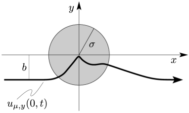
Figure 2: Illustration of a vortex trajectory ${\bf u}_{\mu}(0,t)$ with a finite impact parameter $u_{\mu,y}(z=0,t=-\infty)=-b$, approaching a defect with pinning potential of width $\sigma$ located at ${\bf R}_{p}=(0,0)$. For a strong pinning center, trapping and depinning are strongly asymmetric, what gives rise to a finite pinning force $\langle F_{p}(v)\rangle$.

For a dilute density $n_{p}$ of pinning defects with moderately to strong pinning forces but trapping no more than one vortex at a time, we can reduce the sum over $i$ in Eq. (5) and the sum over $\mu$ in Eq. (6) to only one term each; we call this the single-pin–single-vortex limit which will provide us with results correct to order $n_{p}$. With the vortex $\mu$ impinging on the defect at $({\bf R_{p}},z_{p})$, we have to find the displacement field

$$u_{\nu,\alpha}(z,t) = v_{\alpha}t+\int dt^{\prime}\,G_{\alpha\beta}({\bf R}_{\nu}-{\bf R}_{\mu},z-z_{p},t-t^{\prime})$$ (8)

$$\qquad\times f_{p,\beta}\bigl{[}{\bf R}_{\mu}+{\bf u}_{\mu}(z_{p},t^{\prime})-{\bf R}_{p}\bigr{]}.$$

Once we have (self-consistently) solved the dynamical equation for the displacement field $u_{\mu,\alpha}(z_{p},t)$,

$$u_{\mu,\alpha}(z_{p},t) = v_{\alpha}t+\int dt^{\prime}\,G_{\alpha\alpha}(0,t-t^{\prime})$$ (9)

$$\qquad\times f_{p,\alpha}\bigl{[}{\bf R}_{\mu}+{\bf u}_{\mu}(z_{p},t^{\prime})-{\bf R}_{p}\bigr{]},$$

we can find the full displacement field $u_{\nu,\alpha}(z,t)$ by simple integration of Eq. (8). In Eq. (9), we have used that the Green’s function $G_{\alpha\beta}({\bf r}=0,t)$ is diagonal.

Next, we simplify the expressions for $\langle{\bf F}_{p}\rangle$ and $u_{\mu,\alpha}(z_{p},t)$, Eqs. (5) and (9), in the single-pin–single-vortex approximation. We choose a representative vortex at ${\bf R_{\mu}}={\bf R}$ and a pin at ${\bf r}_{p}$ and rewrite the average pinning-force density Eq. (5) in the form

$$\langle{\bf F}_{p}\rangle = -\frac{n_{p}}{Na_{0}^{2}L}\int\frac{d^{2}R}{a_{0}^{2}}\int dz\,\int d^{3}r_{p}$$

$$\quad\times{\bf f}_{p}\bigl{[}{\bf R}-{\bf R}_{p}+{\bf u}({\bf R}-{\bf R}_{p},z,t)\bigr{]}\delta(z-z_{p}),$$

where we have replaced the sums over $\mu$ and $i$ by the integrations over $d^{2}R/a_{0}^{2}$ and $n_{p}d^{3}r_{p}$. We can choose the pin location $({\bf R}_{p},z_{p})$ at the origin and cancel the integral over ${\bf r}_{p}$ against the volume $Na_{0}^{2}L$ to arrive at

$$\langle{\bf F}_{p}(v)\rangle = -n_{p}\int\frac{d^{2}R}{a_{0}^{2}}\,{\bf f}_{p}\bigl{[}{\bf R}+{\bf u}({\bf R},0,t)\bigr{]}.$$ (11)

Furthermore, we note that we can rewrite the displacement field in Eq. (9) in the form ${\bf u}({\bf R},0,t)={\bf v}t+{\bf u}_{p}({\bf R}+{\bf v}t)$, where the pinning-induced part ${\bf u}_{p}$ of the displacement ${\bf u}$ obeys the equation

$$u_{p,\alpha}({\bf R}+{\bf v}t) = \int dt^{\prime}\,G_{\alpha\alpha}(0,t-t^{\prime})$$

$$\qquad\times f_{p,\alpha}\bigl{[}{\bf R}+{\bf v}t^{\prime}+{\bf u}_{p}({\bf R}+{\bf v}t^{\prime})\bigr{]}.$$

The force in Eq. (11) can be written as ${\bf f}_{p}\bigl{[}{\bf R}+{\bf v}t+{\bf u}_{p}({\bf R}+{\bf v}t)\bigr{]}$ and thus only depends on the combined argument ${\bf R}+{\bf v}t$, the distance between the vortex and the pin at time $t$.

Next, we simplify our task by considering a geometry (see Fig. 2) with impact parameter $b=0$, i.e., a vortex hitting the pin head-on. The average pinning force for this situation can be written as (see Eq. (11))

$$\langle f_{p}(v)\rangle \approx -\int\frac{dx}{a_{0}}\,f_{p}\bigl{[}x+vt+u_{p}(x+vt)\bigr{]}.$$ (13)

This expression can be further simplified, on the one hand, by selecting convenient references for the position $x$ and the time $t$, on the other hand, by choosing between space and time averaging. Specifically, we change space to time average, $dx\to vdt$, and then set $x=0$, what corresponds to choosing our reference position such that the unperturbed vortex passes the pin at time $t=0$. Using $u(vt)=vt+u_{p}(vt)$, we arrive at the final result for the average pinning force

$$\langle f_{p}(v)\rangle \approx -\int\frac{dx}{a_{0}}f_{p}\bigl{[}u(x)\bigr{]},$$ (14)

where the displacement field $u(x=vt)=u_{\mu,x}(0,t)$ obeys the self-consistent dynamical equation Eq. (9) in the simplified form

$$u(x)=x+\int_{-\infty}^{x}\frac{dx^{\prime}}{v}\,G[0,(x-x^{\prime})/v]\,f_{p}[u(x^{\prime})].$$ (15)

In Eq. (15), we have made use of causality, forcing the Green’s function to vanish at negative times $t-t^{\prime}<0$. The coordinate $x=vt$ denotes the asymptotic position of the vortex at $z=\pm\infty$ (replacing $u$ by $u-x$ produces the displacement field defined in Ref. [blatter_04, ]) and we have used the simplified notation $G=G_{xx}$ and $f_{p}=f_{p,x}$ for the force along $x$.

In order to find the mean pinning-force density $\langle F_{p}(v)\rangle$, we have to perform an additional average over the impact parameter $b=y$ of the vortex on the pin in Eq. (11), see Fig. 2. This task is dealt with by equally treating all trajectories within the transverse trapping range $t_{\perp}(v)$ of the pin; this can be done exactly in the static limit blatter_04 , see below, and is a good approximation at finite velocities where $t_{\perp}(v)$ depends on $v$ as discussed in Sec. IV.5. As a result, the average over $b$ contributes a factor $2t_{\perp}(v)/a_{0}$ and the $y$ component of the force averages to zero. We then obtain the final expression for the mean pinning-force density $\langle F_{p}(v)\rangle$ along $x$ in the form

$$\langle F_{p}(v)\rangle \approx n_{p}\frac{2t_{\perp}(v)}{a_{0}}\langle f_{p}(v)\rangle.$$ (16)

The equations (14), (15), and (16) together with the dynamical equation (1) define the simplified problem which now is amenable to a complete (numerical) solution.

The local dynamical Green’s function $G(t)\equiv G_{xx}({\bf r}=0,t)$ is obtained from the Fourier transform $G_{xx}$ as given by Eq. (II). We neglect the compression modes as compared to the softer shear modesblatter_94 to find (the average of $K_{y}^{2}/K^{2}$ over the Brillouin zone leads to the overall factor 1/2 which has been ignored in Ref. [blatter_94, ])

$$G(t)=\Theta(t)\frac{1}{2\eta}\int_{\mathrm{BZ}}\frac{d^{3}k}{(2\pi)^{3}}e^{-[c_{66}K^{2}+c_{44}({\bf k})k_{z}^{2}]t/\eta}.$$ (17)

Depending on the time $t$, the integral is either cut by the exponential or by the Brillouin zone boundary (we use a circularized Brillouin zone with $K_{\rm\scriptscriptstyle BZ}^{2}=4\pi/a_{0}^{2}$); in addition, the dispersive nature of the tilt modulus has to be accounted for within an intermediate-time regime.

In the static limit, it is the local static elastic Green’s function $G({\bf r}=0,\omega=0)=\int_{0}^{\infty}dt\,G(0,t)$ which plays an important role; the latter defines an effective elasticitywilla_16 through $\bar{C}=1/G(0,0)$,

$$\bar{C}\approx\nu\frac{a_{0}^{2}}{\lambda}\sqrt{c_{66}c_{44}}\approx 4\sqrt{\pi}\frac{\varepsilon_{0}}{a_{0}},$$ (18)

where we have used the numerical $\nu=4$ (but note [com_nu, ]) and $\varepsilon_{0}=(\Phi_{0}/4\pi\lambda)^{2}$ denotes the characteristic line energy of a vortex.

The characteristic time separating different dynamical regimes is given by the thermal time

$$t_{\mathrm{th}}=\frac{\eta}{c_{66}K_{\rm\scriptscriptstyle BZ}^{2}}\approx\frac{4\eta a_{0}^{3}}{\sqrt{\pi}\bar{C}},$$ (19)

the dissipative relaxation time of short-scale elastic deformations blatter_94 . At long times $t>t_{\mathrm{th}}(\lambda/a_{0})^{2}$, the integral in (17) is cut by the exponential at small values of $K$ such that the dispersion in $c_{44}$ can be neglected; with $c_{44}\approx B^{2}/4\pi$ and $c_{66}\approx\Phi_{0}B/(8\pi\lambda)^{2}$ one finds the 3D Green’s function blatter_94

$$G^{\rm\scriptscriptstyle 3D}[t_{\mathrm{th}}(\lambda/a_{0})^{2}\ll t]) \approx \frac{1}{2\pi}\frac{a_{0}}{\lambda}\frac{1}{\bar{C}t_{\mathrm{th}}}\left(\frac{t_{\mathrm{th}}}{t}\right)^{3/2}\!\!,$$ (20)

describing a response $G^{\rm\scriptscriptstyle 3D}(t)\propto t^{-d/2}$ involving the entire $d=3$ bulk vortex system. At intermediate times $t_{\mathrm{th}}(\lambda/a_{0})^{2}>t>t_{\mathrm{th}}$, the dispersion $c_{44}\approx B^{2}/4\pi\lambda^{2}K^{2}$ in the tilt modulus becomes relevant and the response is that of a dispersive elastic manifold with an elastic Green’s function behaving as the one of a 4D non-dispersive medium, blatter_94

$$G^{\rm\scriptscriptstyle 4D}[t_{\mathrm{th}}\ll t\ll t_{\mathrm{th}}(\lambda/a_{0})^{2}] \approx \frac{1}{2\bar{C}t_{\mathrm{th}}}\left(\frac{t_{\mathrm{th}}}{t}\right)^{2}\!\!\!.$$ (21)

For short times $t<t_{\mathrm{th}}$, the integral is cut by the Brillouin-zone boundary. This short-time response attains to the dynamics of an individual vortex line blatter_94 (in this 1D limit both, longitudinal and transverse parts of the Green’s function Eq. (II), contribute)

$$G^{\rm\scriptscriptstyle 1D}(t\ll t_{\mathrm{th}}) \approx \Theta(t)\frac{2}{\sqrt{\pi}}\frac{1}{\bar{C}t_{\mathrm{th}}}\left(\frac{t_{\mathrm{th}}}{t}\right)^{1/2}.$$ (22)

Note that the time integral in Eq. (15) is well behaved as the Green’s function is regular (integrable) at long times (since $G^{\rm\scriptscriptstyle 3D}\propto t^{-3/2}$) as well as at short times (since $G^{\rm\scriptscriptstyle 1D}\propto t^{-1/2}$), with the main contribution to the time integral originating from $t_{\mathrm{th}}$.

III Static solution

The critical pinning-force density $F_{c}$ is obtained in two steps, where the first determines the pinning-force average $f_{c}$ (longitudinal average) and the second finds the transverse trapping length $t_{\perp}$ (transverse average).

III.1 Longitudinal average $f_{c}$

In the static situation, the self-consistent integral equation (15) turns into the simpler algebraic equation

$$u_{s}(x)=x+{f_{p}[u_{s}(x)]}/{\bar{C}}.$$ (23)

Solving Eq. (23) self-consistently for $u_{s}(x)$ and inserting the result into Eq. (14), we obtain the critical force

$$f_{c}=\langle f_{p}(v=0)\rangle=-\int\frac{dx}{a_{0}}\,f_{p}[u_{s}(x)].$$ (24)

The static self-consistency equation (23) can be lifted to a total energy: we define the total pinning energy $e_{t}(x)$ as the sum of elastic and pinning energies, see Fig. 3(d),

$$e_{t}(x)\equiv e_{t}[x;u_{s}(x)]=\frac{\bar{C}}{2}[u_{s}(x)-x]^{2}+e_{p}[u_{s}(x)],$$ (25)

then the total derivative of $e_{t}(x)$ can be written in the form

$$\frac{de_{t}(x)}{dx}=-\bar{C}(u_{s}-x)+\partial_{x}u_{s}[\bar{C}(u_{s}-x)-f_{p}(u_{s})]$$

and using Eq. (23), we find that

$$f_{p}[u_{s}(x)]=-\frac{de_{t}(x)}{dx}.$$ (26)

At weak pinning, the effective static pinning force $f_{p}[u_{s}(x)]$ appearing in Eq. (24) is a single-valued smooth function, resulting in a vanishing force average

$$f_{c}=\int\frac{dx}{a_{0}}\frac{de_{t}(x)}{dx}=\frac{e_{t}(\infty)-e_{t}(-\infty)}{a_{0}}=0.$$ (27)

A finite critical force-density $F_{c}\propto n_{p}^{2}$ then is established through fluctuations in the defect density as described through weak collective pinning theory.

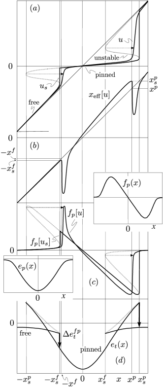
Figure 3: Sketch of the static and dynamic displacement fields $u_{s}(x)$ and $u(x)$ (a). The static displacement $u_{s}(x)$ jumps from the free to the pinned branch at $-x_{s}^{f}$ and back to the free branch at $x_{s}^{p}$. In the smooth dynamic displacement $u(x)$, these jumps are replaced by sharp rises at the shifted positions $-x^{f}$ and $x^{p}$. Below, we will make use of a smooth multi-valued static solution $\bar{u}_{s}$ where the jumps are replaced by the unstable branch $u_{s}^{u}$ (dotted). The dotted arrows refer to the shift $x_{\mathrm{eff}}[u](x)$, see (b), that connects the smooth static and dynamic solutions $\bar{u}_{s}(x)$ and $u(x)$, respectively. (b) Effective coordinate $x_{\mathrm{eff}}[u](x)=x-\delta x[u](x)$ allowing to express the dynamic solution through the static one, $u(x)=\bar{u}_{s}[x_{\mathrm{eff}}[u](x)]$. (c) Static and dynamic force profiles $f_{p}[u_{s}(x)]$ and $f_{p}[u(x)]$. (d) Static total energy profile $e_{t}(x)$. The insets show the bare force and energy profiles of the pinning center.

A strong pin producing a finite average pinning-force density $\propto n_{p}$ is characterized by the appearance of bistable solutions (or branches) in the single-pin problem Eq. (23). The critical force $f_{c}$ then depends on the occupation of these branches, with an asymmetric occupation of the solutions resulting in a finite average force. Indeed, when typical values of $f_{p}/\sigma\bar{C}$ become large, the bare pinning force $f_{p}(x)$, see inset of Fig. 3(c), when evaluated at the shifted position $u_{s}(x)$, is tilted backward, see Fig. 3(c). In this strong-pinning situation the derivative

$$\partial_{x}u_{s}(x)=\frac{1}{1-\partial_{u}f_{p}\bigl{[}u_{s}(x)\bigr{]}/\bar{C}}$$ (28)

diverges at the positions $\pm x_{s}^{f}$ and $\pm x_{s}^{p}$ where $\partial_{u}f_{p}[u_{s}(x)]=\bar{C}$, signalling the appearance of multiple solutions with pinned ($u_{s}^{p}(x)$), unstable ($u_{s}^{u}(x)$), and free ($u_{s}^{f}(x)$) or unpinned branches, see Fig. 3. Strong pinning then requires the ratio

$$\kappa=\max_{x}\{\partial_{u}f_{p}[u_{s}(x)]\}/\bar{C}=\max_{x}[f_{p}^{\prime}(x)]/\bar{C}$$ (29)

to be larger than one, $\kappa>1$; this is the famous Labusch criterion for strong pinning labusch_69 . A vortex incident from the left onto the defect and moving towards the right will leave the free branch $u_{s}^{f}(x)$ at $-x_{s}^{f}$ and jump to the pinned branch $u_{s}^{p}(x)$ (see Fig. 3(a), the unstable branch $u_{s}^{u}(x)$ and parts of the pinned branch are jumped over). After crossing the defect, the vortex will depin from the pinned branch at $x_{s}^{p}$ and jump back to the free branch (the points $x_{s}^{f}$ and $-x_{s}^{p}$ are relevant when the vortex moves from right to left). As a result, the critical pinning force $f_{c}$ becomes finite and equal to the sum of energy jumps at $-x_{s}^{f}$ and $x_{s}^{p}$,

$$f_{c}=\!\biggl{[}\int_{-\infty}^{-x_{s}^{f}}\!\!\!\!\!\!\!+\!\int_{-x_{s}^{f}}^{x_{s}^{p}}\!\!\!+\!\!\int_{x_{s}^{p}}^{\infty}\biggr{]}\frac{dx}{a_{0}}\,\frac{de_{t}(x)}{dx}\!=\!\frac{\Delta e_{t}^{fp}\!+\!\Delta e_{t}^{pf}}{a_{0}}$$ (30)

with the positive jumps $\Delta e_{t}^{fp}=e_{t}^{f}(-x_{s}^{f})-e_{t}^{p}(-x_{s}^{f})$ and $\Delta e_{t}^{pf}=e_{t}^{p}(x_{s}^{p})-e_{t}^{f}(x_{s}^{p})$. Hence, it is the asymmetry between jumping into the pinning well at $-x_{s}^{f}$ and out of it at $x_{s}^{p}$ which generates the finite (and actually maximal) pinning force labusch_69 ; larkin_79 ; larkin_86 ; blatter_04 $f_{c}$, see Fig. 3(c). Alternatively, Eq. (30) may be interpreted in a (non-equilibrium) statistical sense in terms of an imbalance between the occupation of the different pinning branches that is produced by the applied Lorentz force.

III.2 Trapping lengths $t_{\perp}$ and $t_{\parallel}$

In order to obtain the critical force-density $F_{c}$, we have to determine the trapping length $t_{\perp}$, see Eq. (16). For a radially symmetric defect potential, this is conveniently done by considering the total energy $e_{t}(R;r)$ for a vortex with radial asymptotic and tip positions $R$ and $r$, see Eq. (25),

$$e_{t}(R;r)=\frac{\bar{C}}{2}(r-R)^{2}+e_{p}(r).$$ (31)

Plotting this function at fixed $R$ versus $r$, one observes a single (pinned) minimum in the variable $r$ for $0<R<R_{s}^{f}$, two minima (pinned and free) when $R_{s}^{f}<R<R_{s}^{p}$, and again a single (free) minimum for $R>R_{s}^{p}$, see Fig. 4; these minima determine the (static) tip position $r_{s}(R)$ at given asymptotic position $R$; indeed, the condition $\partial_{r}e_{t}(R;r)=0$ at fixed $R$ reproduces Eq. (23) in the form $r=R+f_{p}(r)/\bar{C}$ and interrelates asymptotic ($R$) and tip ($r$) positions of the vortex. The appearance or disappearance of these minima at $R_{s}^{f}~{}(=x_{s}^{f})$ and $R_{s}^{p}~{}(=x_{s}^{p})$ signals the beginning or ending of the free and pinned branches. At these points, the second derivative $\partial^{2}_{r}e_{t}(R;r)=0$ vanishes as well, i.e., the curvatures in the elastic and pinning term of Eq. (31) compensate and hence

$$\partial_{r}f_{p}(r)|_{r(R_{s}^{f,p})}=\bar{C}.$$ (32)

The latter condition actually determines the critical tip positions $r_{s}^{f}=r(R_{s}^{f})$ and $r_{s}^{p}=r(R_{s}^{p})$, while the corresponding asymptotic positions $R_{s}^{f}$ and $R_{s}^{p}$ are obtained from solving the force balance equation $r=R+f_{p}(r)/\bar{C}$.

Figure 4: Total energy $e_{t}(R;r)$ providing the configurational energy of a vortex at the asymptotic distance $R$ from the pin when its tip resides at the distance $r$. Minimizing $e_{t}(R;r)$ at fixed $R$ with respect to $r$ defines the static tip position $r_{s}(R)$. Dotted lines trace the pinning potential $e_{p}(r)$ and the elastic energy $\bar{C}r^{2}/2$. Solid lines show the situation for a), $R_{s}^{f}<R=R_{a}<R_{s}^{p}$ with two minima, just before the vortex in the free minimum jumps into the pin at $R_{s}^{f}=x_{s}^{f}$, b), $R_{s}^{f}<R=R_{b}<R_{s}^{p}$ with two minima just before depinning at $R_{s}^{p}=x_{s}^{p}$, and c), $R=R_{c}>R_{s}^{p}$ with one (free) minimum just after depinning at $R_{s}^{p}$.

In the static situation, a vortex approaching the defect gets trapped as soon as it enters the circle at $R_{s}^{f}$: as the free branch ends at $R_{s}^{f}$, the vortex tip falls into the stable minimum at $r(R_{s}^{f})$ which resides on the pinned branch, see curve a) in figure 4. Hence, all vortices impacting the defect within a distance $R_{s}^{f}$ will get trapped and we find that

$$t_{\perp}=R_{s}^{f}=x_{s}^{f},$$ (33)

see also Ref. [blatter_04, ]. Similarly, the vortices remain trapped by the pin until the asymptotic position $R_{s}^{p}$ is reached and we obtain the longitudinal trapping length

$$t_{\parallel}=R_{s}^{p}=x_{s}^{p}.$$ (34)

Hence, the mathematical objects $\pm x_{s}^{f}$ and $\pm x_{s}^{p}$ denoting the positions where the slope $\partial_{x}u_{s}(x)$ of the static displacement diverges determine the physical lengths $t_{\perp}$ and $t_{\parallel}$ where the vortices get and remain trapped, respectively.

Finally, we combine the results Eq. (30) for the critical pinning force and Eq. (33) for the transverse trapping length into the expression for the critical-force density $F_{c}$, see Eq. (16), and obtain

$$F_{c}=\frac{2x_{s}^{f}}{a_{0}^{2}}n_{p}[\Delta e_{t}^{fp}+\Delta e_{t}^{pf}].$$ (35)

III.3 Universal static solution for very strong pinning $\kappa\gg 1$

It turns out, that the above general considerations can be pushed further in the limit of very strong pinning $\kappa\gg 1$, where a universal solution is available that is independent of the details of the pinning potential shape. We start from Eq. (23) by noticing that for the pinned situation, the last term $f_{p}[u_{s}(x)]/\bar{C}$ is large and has to be compensated by the coordinate $x$, since the tip position $u_{s}(x)$ on the right has to stay within the pin and hence is small, $u_{s}(x)<\sigma$. As a result, we find that for very strong pinning, the static force

$$f_{p}[u_{s}(x)]\approx-\bar{C}x$$ (36)

changes linearly over a wide range until reaching the largest (negative) force $-\bar{C}x_{s}^{p}\approx-f_{p}$ before depinning, see Fig. 5. The latter condition provides an accurate estimate for $x_{s}^{p}$ in the very strong pinning limit,

$$t_{\parallel}=x_{s}^{p}\approx\frac{f_{p}}{\bar{C}}\sim\kappa\sigma,$$ (37)

Since $\kappa\sigma$ is large, the residual force after depinning is very small. Alternatively, the above result can be found by transforming Eq. (28) to its force analogue; taking the derivative of Eq. (23) and using Eq. (28), we find that

$$\frac{df_{p}[u_{s}(x)]}{dx}=-\frac{\bar{C}}{1-\bar{C}/\partial_{u}f_{p}[u_{s}(x)]}.$$ (38)

Again, for strong pinning, we have $\partial_{u}f_{p}[u_{s}(x)]/\bar{C}\gg 1$ over a large range $\sim\kappa\sigma$ along the $x$-axis and hence the force derivative is renormalized to the (constant) effective elasticity $\bar{C}$, see Fig. 5.

Next, we discuss the jumps into and out of the pin at $-x_{s}^{f}$ and at $x_{s}^{p}$—we will need these results later in the discussion of the small velocity corrections to $F_{c}$. We distinguish pins with (long) tails decaying algebraically with $e_{p}(r)\propto(\sigma/r)^{n}$, from compact pins with tails decaying faster than any power, e.g., $e_{p}\propto e^{-r/\sigma}$.

The jumps in and out of the pin are determined by the conditions $\partial_{u}e_{t}(x;u)=0$ and $\partial_{u}^{2}e_{p}(x;u])=0$, see Sec. III.2. For the jump into the pin, we solve $\partial_{u}f_{p}(u)=\bar{C}$, cf. Eq. (32), and find that $u_{s}(-x_{s}^{f})\sim-\kappa^{1/(n+2)}\sigma$ for a pin with tails and $u_{s}(-x_{s}^{f})\sim-\sigma\ln\kappa$ for a compact pin. The associated asymptotic vortex position $x_{s}^{f}$ follows from Eq. (23); since the jump into the pin takes place at small forces, we can approximate $-x_{s}^{f}\approx u_{s}(-x_{s}^{f})$ and hence

$$t_{\perp}=x_{s}^{f}\sim\kappa^{1/(n+2)}\sigma$$ (39)

for a pin with tails. Similarly, for a compact pin, $x_{s}^{f}\sim\sigma\ln\kappa$. The result for the vortex jumping out of the pin has been found above, see Eq. (37).

The pinning force at $-x_{s}^{f}$ can be estimated with the help of Eq. (23): just before the jump, $u_{s}\approx-x_{s}^{f}$ and the force assumes a small value $f_{p}(-x_{s}^{f})\approx f_{p}/\kappa^{(n+1)/(n+2)}$, while after the jump, $|u_{s}|\ll x_{s}^{f}$ and hence $f_{p}(u_{s})\approx\bar{C}x_{s}^{f}\sim f_{p}\kappa^{1/(n+2)-1}$, which is of the same order. For a compact pin, the force before the jump is $f_{p}/\kappa$ and assumes a logarithmically larger value after the jump, $(f_{p}/\kappa)\ln\kappa$. When jumping out of the pin, $u_{s}(x_{s}^{p})\approx\sigma$ and the pinning force goes from $-f_{p}$ before the jump to very small values thereafter, $\sim-f_{p}/\kappa^{n+1}$ and $-f_{p}e^{-\kappa}$ for pins with tails and for compact pins, respectively.

Figure 5: (a) Bare and effective static pinning forces $f_{p}(x)$ and $f_{p}[u_{s}(x)]$ for a strong pinning potential. The steep negative slope $\partial_{x}f_{p}(x)$ on the scale $\sigma$ transforms into the flat universal slope $-\bar{C}x$ in $f_{p}[u_{s}(x)]$ on the larger scale $\kappa\sigma$. The rounding before the collapse of $f_{p}[u_{s}(x)]$ at $x_{s}^{p}$ disappears in the limit $\kappa\to\infty$; the jump $\sim f_{p}/\kappa$ into the pin at $-x_{s}^{f}$ is small at large $\kappa$. (b) Vortex deformation for two asymptotic positions $x_{1}$ and $x_{2}$. While $x_{2}-x_{1}$ increases on the scale $\kappa\sigma$ the associated displacements $u_{s1}$ and $u_{s2}$ change on the scale $\sigma$.

The integration over the static force profile $f_{p}[u_{s}(x)]$ provides us with a critical force-density (see Eqs. (24) and (33); note that $f_{p}[u_{s}(x)]\approx-\bar{C}x$ on the pinned branch)

$$F_{c} \approx -n_{p}\frac{2x_{s}^{f}}{a_{0}^{2}}\int_{-x_{s}^{f}}^{x_{s}^{p}}dx\,f_{p}\bigl{[}u_{s}(x)\bigr{]}$$

$$\approx \Bigl{(}\frac{x_{s}^{f}+x_{s}^{p}}{a_{0}}\Bigr{)}^{2}n_{p}x_{s}^{f}\bar{C}\approx\frac{\kappa\sigma x_{s}^{f}}{a_{0}^{2}}n_{p}f_{p},$$

where we have used $x_{s}^{p}\sim\kappa\sigma\gg x_{s}^{f}$ and $\kappa\sim f_{p}/\sigma\bar{C}$ in the last estimate. The result involves, besides the maximal force $f_{p}$ and density $n_{p}$ of pins, the trapping areaivlev_91 ; blatter_04

$$S_{\mathrm{trap}}=2t_{\perp}t_{\parallel}\sim 2x_{s}^{f}\,\kappa\sigma.$$ (41)

With $\kappa\sim f_{p}/\sigma\bar{C}$ and $\bar{C}\sim\varepsilon_{0}/a_{0}$, see Eqs. (29) and (18), we obtain a field dependence $F_{c}\propto B^{(n+1)/2(n+2)}$ for the critical force $F_{c}$, assuming a pin with tails.ivlev_91 For large $n$, this produces the typical strong-pinning field-dependence $j_{c}\propto 1/\sqrt{B}$ for the critical current density, which is cutoff at small fields when bulk 3D strong pinning crosses over to single-vortex 1D strong pinning at $n_{p}a_{0}\xi^{2}\kappa\sim 1$.blatter_04

III.3.1 Corrections to the universal static solution

Let us improve the accuracy of the above analysis and further investigate the behavior of the vortex near depinning. In order to find the static force profile $f_{p}[u_{s}(x)]$ near depinning at $x_{s}^{p}$, we make use of Eq. (23) and expand the bare potential $f_{p}(x)$ in the relevant region around its minimum (near the maximal pinning force pointing along $-x$). We characterize the minimum in the bare pinning force $f_{p}(x)$ (i.e., its largest negative value) through its position $\sigma_{m}$, the maximum (negative) pinning force $-f_{p}$, and the (positive) curvature $f_{p}^{\prime\prime}=f_{p}/\sigma^{2}$,

$$f_{p}(x)\approx-f_{p}+\frac{f_{p}}{2\sigma^{2}}(x-\sigma_{m})^{2}.$$ (42)

Note that, here, the parameter $\sigma\equiv(f_{p}^{\prime\prime}(\sigma_{m})/f_{p})^{1/2}$ is a precisely defined model parameter that agrees with the previous (loose) definition as the pin size for the situation where the defect potential involves only one length scale. In order to relate the static displacement field $u_{s}$ to the asymptotic coordinate $x$, we combine the above Ansatz for the bare pinning force $f_{p}(x)$ with the static self-consistency equation (23). Replacing $x\to u_{s}$ in Eq. (42) and using (23), $\bar{C}(u_{s}-x)=f(u_{s})$, we find the static displacement field

$$u_{s}(x)\approx\sigma_{m}+\frac{\sigma}{\bar{\kappa}}-\sqrt{\frac{2\sigma}{\bar{\kappa}}(x_{s}^{p}-x)}$$ (43)

with $\bar{\kappa}\equiv f_{p}/\sigma\bar{C}$ and $x^{p}_{s}\equiv\bar{\kappa}\sigma+\sigma_{m}+\sigma/2\bar{\kappa}\approx\bar{\kappa}\sigma$ the depinning point, see Fig. 5. Making use of Eq. (23) once more, we obtain the static pinning force

$$f_{p}[u_{s}(x)] \approx -\bar{C}x+f_{p}\frac{u_{s}(x)}{\bar{\kappa}\sigma},$$ (44)

with the last term a correction of order $\sim f_{p}/\bar{\kappa}$. This force profile decreases linearly with slope $\bar{C}$ up to $x\approx\bar{\kappa}\sigma$, reaches its minimum $-f_{p}$ (the maximum backward force $f_{p}$) at $x=\bar{\kappa}\sigma+\sigma_{m}$ and increases by $f_{p}/2{\bar{\kappa}}^{2}$ when $x$ increases further by $\sigma/2\bar{\kappa}$ in order to diverge upwards at $x=x_{s}^{p}$, see Fig. 5.

In summary, at very strong pinning (by a defect with tails), we find a universal static solution where the vortex jumps into the pin at $-x_{s}^{f}\sim-\kappa^{1/(n+2)}\sigma$ and then is deformed linearly in $x$, with the vortex tip remaining trapped in the pin. The elastic energy of this deformation balances the effective pinning force $-\bar{C}x$. The backward pointing tip remains fixed onto the defect until reaching the largest force $-f_{p}$ with the vortex stretched by $\sim\kappa\sigma$, see Fig. 5. When the force decreases again in magnitude, the vortex remains attached to the pin over the short distance $\sim\sigma/2\kappa$ and then depins with a sharp forward jump in $u_{s}(x)$ at $x_{s}^{p}$, from $u_{s}\sim\sigma$ before to $u_{s}\sim\kappa\sigma$ after depinning. With this jump, the vortex tip depins and ends on the free branch where it experiences a small residual force $f_{p}(x_{s}^{p})\sim-f_{p}/\kappa^{n+1}<0$. For a vortex with a finite impact parameter and a radially symmetric defect potential, the above scenario is still valid, with the vortex jumping into and out of the pin at the radii $R_{s}^{f}=x_{s}^{f}$ and $R_{s}^{p}=x_{s}^{p}$. Note that at very strong pinning, jumping into and out of the pin are very asymmetric processes, with the vortex jumping into the pin anywhere along the semicircle with radius $R_{s}^{f}$, while it jumps out of the pin in a narrow, forward directed angle, see Fig. 2. Hence the depinning process (that determines $\langle f_{p}(v)\rangle$) does not depend much on the impact parameter $b$.

III.4 Static solution for moderately strong pinning $\kappa\gtrsim 1$

A similarly accurate analysis can be done at moderate pinningblatter_04 . Expanding the pinning potential $e_{p}(x)$ around the point $\sigma_{mc}$ of maximal negative curvature, $e_{p}^{{}^{\prime\prime}}(x)=-\bar{C}\kappa+\alpha(x-\sigma_{mc})^{2}/2$, the transition to weak pinning can be described within the Landau formulation of a magnetic phase transition and one finds the resultblatter_04

$$F_{c} \approx 18\frac{x_{s}^{f}}{a_{0}^{2}}n_{p}\frac{\bar{C}^{2}}{e_{p}^{{}^{\prime\prime\prime\prime}}}(\kappa-1)^{2}\sim\frac{\sigma x_{s}^{f}}{a_{0}^{2}}n_{p}f_{p}(\kappa-1)^{2},$$ (45)

with $e_{p}^{{}^{\prime\prime\prime\prime}}|_{\sigma_{mc}}=\alpha$. In the last relation, we have used the estimate $\alpha\sim f_{p}/\sigma^{3}$ and $\bar{C}^{2}/\alpha\sim f_{p}\sigma$ with $\kappa$ close to unity.

IV Dynamic solution

Once the Lorentz force density $F_{\rm\scriptscriptstyle L}$ in Eq. (1) increases beyond the critical force $F_{c}$, the mean velocity $v$ becomes finite. According to Eq. (15), the deformation $u(x)$ of the vortex is determined by the pinning force $f_{p}[u(x^{\prime})]$ averaged over (past) times $t^{\prime}=x^{\prime}/v$ and weighted by the local dynamical Green’s function $G(0,(x-x^{\prime})/v)$. The average pinning force $\langle f_{p}(v)\rangle$, Eq. (14), then depends on the mean velocity $v$, starting at $f_{c}$ for $v=0$ and vanishing at large velocities $v$ as the pins only weakly disturb the fast flow of vortices. Given the time scale $t_{\mathrm{th}}$ of $G(0,t)$ and the pinning scale $\kappa\sigma$ over which the force $f_{p}[u(x^{\prime})]$ remains finite, we can estimate the pinning velocity

$$v_{p}=\frac{\kappa\sigma}{t_{\mathrm{th}}}\sim\frac{f_{p}}{\eta\,a_{0}^{3}}$$ (46)

where dynamical effects start to modify $\langle f_{p}(v)\rangle$. The last expression describes the typical velocity scale of a vortex segment of length $a_{0}$ (the vortex tip) moving in the pinning potential $e_{p}(r)$, $\eta_{l}a_{0}\dot{r}\sim f_{p}$ and $\eta_{l}=a_{0}^{2}\eta$ the line viscosity of a vortex.

Given the form of the pinning potential $e_{p}(r)$, the straightforward integration of the dynamical equation (15) gives us access to the average pinning force $\langle f_{p}(v)\rangle$ for any velocity $v$ and the calculation of $t_{\perp}(v)$ provides us with the pinning-force density $\langle F_{p}(v)\rangle$ via Eq. (16). Analytic results, instead, have to be obtained using different approaches that depend on the velocity $v$: At high velocities, we use perturbation theory away from flux flow and directly address the force density $\langle F_{p}(v)\rangle$, in the intermediate velocity regime that is present at large values of $\kappa$, we determine the average force $\langle f_{p}(v)\rangle$ via construction of a self-consistent solution for $f_{p}[u(x)]$, while at low velocities, we find again the average $\langle f_{p}(v)\rangle$ using a perturbative approach, this time away from the static solution. The intermediate and small velocity results then have to be completed with a calculation of $t_{\perp}(v)$.

IV.1 Overview on pinning-force averages

We first present the results obtained from a numerical forward integration of Eq. (15) for a Lorentzian shaped pinning potential (we assume non-dispersive moduli corresponding to a field $B\sim\Phi_{0}/\lambda^{2}$). In Fig. 6, we show the scaled average pinning force $\langle f_{p}(v)\rangle a_{0}^{2}/e_{p}\xi$ versus the scaled velocity $v/v_{p}$.

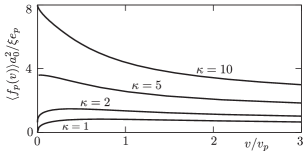
Figure 6: Velocity-dependence of the pinning-force density $\langle f_{p}(v)\rangle$ for Lorentzian pins $e_{p}(r)=-e_{p}/(1+r^{2}/2\xi^{2})$ with Labusch parameters ranging from $\kappa=1$ to $\kappa=10$; the typical depinning velocity scale $v_{p}$ where the pinning force changes depends on the Labusch parameter $\kappa$. We haven chosen a field $B=\Phi_{0}/\lambda^{2}$, $a_{0}=\lambda$, such that the elastic moduli are non-dispersive. While the pinning force decreases monotonically for large $\kappa$, it first increases at small velocities for $\kappa\gtrsim 1$ before eventually decreasing at large velocities. Original figure published in Ref. [thomann_12, ].

Varying the pinning energy $e_{p}$ at fixed size $\sigma$, we follow the evolution of the average pinning force $\langle f_{p}(v)\rangle$ from very strong pinning $\kappa=10$ to moderately strong pinning at $\kappa\gtrsim 1$. With $e_{p}\sim H_{c}^{2}\xi^{3}\sim\varepsilon_{0}\xi$ ($H_{c}$ the thermodynamic critical field) the Labusch parameter can naturally access large numbers $\kappa\sim f_{p}/\xi\bar{C}\sim(e_{p}/\xi\varepsilon_{0})(a_{0}/\xi)\sim a_{0}/\xi\gg 1$. For very strong pinning, the critical force $f_{c}=\langle f_{p}(v=0)\rangle$ is large and the pinning force $\langle f_{p}(v)\rangle$ decreases when vortices start moving. On approaching the Labusch point $\kappa=1$ and for weak pinning ($\kappa<1$, not shown) the critical force vanishes and $\langle f_{p}(v)\rangle$ increases with $v$; this increase is trivially understood as the pinning force cannot turn negative. The vanishing of $f_{c}$ on approaching $\kappa=1$ follows a quadratic behaviorlabusch_69 ; blatter_04 , $f_{c}\propto(\kappa-1)^{2}$, see (45).

In order to understand the rough functional form of $\langle f_{p}(v)\rangle$ at small and large velocities $v$, we start from Eq. (14) and expand it about the static ($u_{s}(x)$) and dynamic ($u(x)\approx x=vt$) solutions of Eq. (15), respectively. In the static limit $v=0$, $f_{p}[u_{s}(x^{\prime})]$ can be taken out of the integral in Eq. (15); the remaining integral draws its main contribution from times $t\sim t_{\mathrm{th}}$, $\int dt\,G\sim t_{\mathrm{th}}\,G^{\rm\scriptscriptstyle 1D}(t_{\mathrm{th}})\sim 1/\bar{C}$, see Eq. (22). The velocity correction at small $v$ then derives from cutting this time integral at large but finite times $t_{v}\sim\kappa\sigma/v$, as the pinning force $f_{p}[u(x^{\prime}=vt^{\prime})]$ vanishes when the vortex leaves the pin at $t_{v}$. For $t_{v}>t_{\mathrm{th}}$ or $v<v_{p}$, the integral still picks up its main contribution near $t_{\mathrm{th}}$ that produces the static displacement $u_{s}(x)$; the correction $\int_{t_{v}}^{\infty}dt\,G^{\rm\scriptscriptstyle 3D}(t)\sim\sqrt{vt_{\mathrm{th}}/\kappa\sigma}/\bar{C}$ scales with $\sqrt{v/v_{p}}$ and hence $\langle f_{p}(v)\rangle-f_{c}\propto\sqrt{v/v_{p}}$ at small velocities. Note, that a more refined discussion (see Sec. IV.4 below) is required in order to explain the sign change in the derivative of $\langle f_{p}(v\to 0)\rangle$ with decreasing $\kappa$, see Fig. 6.

In the limit of very high velocity $v$, the displacement $u(x)\approx vt$ and the force (14) vanishes since $\int dxf_{p}(x)=0$. Corrections derive from the second term in Eq. (15), where the time integral now is cut on $t_{v}\sim\sigma/v\ll t_{\mathrm{th}}$. This implies that the entire pinning force derives from the integral at short times, $\int_{0}^{t_{v}}dt\,G^{\scriptscriptstyle 1D}(t)\sim\sqrt{\sigma/vt_{\mathrm{th}}}/\bar{C}$, and hence the pinning force vanishes as $\langle f_{p}(v)\rangle\propto\sqrt{v_{p}/v}$, resulting in a monotonic decrease of $\langle f_{p}(v)\rangle$ for large values of $\kappa$. For small values of $\kappa$, i.e., $\kappa\to 1$, the vanishing of the critical force $f_{c}=\langle f_{p}(v=0)\rangle\propto(\kappa-1)^{2}$ implies first an increase of the pinning-force density $\langle f_{p}(v)\rangle-f_{c}\propto\sqrt{v/v_{p}}$ at small $v$ which is later followed by the decrease $\propto\sqrt{v_{p}/v}$ at large $v$, resulting in the non-monotonic behavior of $\langle f_{p}(v)\rangle$ shown in Fig. 6.

In the above very high velocity regime, the pinning-induced correction $u_{p}\sim f_{p}\sqrt{\sigma/vt_{\mathrm{th}}}/\bar{C}\sim\sigma\sqrt{\kappa v_{p}/v}$ should be small, $u_{p}<\sigma$, and thus $v>\kappa v_{p}$. This leaves a large intermediate velocity regime $v_{p}<v<\kappa v_{p}$ where neither of the above perturbative approaches can be applied. Understanding this intermediate velocity regime requires a more elaborate analysis of Eq. (15). Within this region, the two terms on the right are large and nearly compensate one another to produce a tip position $u(x)\lesssim\sigma$ within the pin. Hence, Eq. (15) can be written in the form

$$-vt\approx\int_{-\infty}^{t}dt^{\prime}G(0,t-t^{\prime})f_{p}[u(t)],$$ (47)

where we have replaced space by time coordinates. Using the 1D Green’s function (22), we estimate the right hand side as $\sqrt{t/t_{\mathrm{th}}}f_{p}[u(t)]/\bar{C}$ and therefore $f_{p}[u(t)]\sim-v\sqrt{t\,t_{\mathrm{th}}}\bar{C}$. The linear static force $f_{p}[u_{s}(x)]\approx-\bar{C}x$ of Eq. (36) then transforms into a square-root dynamic force

$$f_{p}[u(x)]\sim-\bar{C}\,\sqrt{x\sigma}\sqrt{v/v_{\sigma}}.$$ (48)

The maximal pinning force $-f_{p}$ is reached at $x\sim\kappa\sigma(v_{p}/v)$, reduced by a factor $v_{p}/v$ with respect to the maximal pinning length $x_{s}^{p}\sim\kappa\sigma$ at vanishing velocity. The above results smoothly interpolate between those found in the small and large velocity regions at $v<v_{p}$ and $v>\kappa v_{p}$, respectively. Furthermore, one easily convinces oneself that the pinning time $t_{v}\sim\kappa\sigma v_{p}/v^{2}<t_{\mathrm{th}}$ within this velocity region, justifying the use of the 1D Green’s function. Integrating the pinning force (48) over the reduced pinning length $t_{\parallel}\kappa\sigma\sqrt{v_{p}/v}$, we obtain a decaying average pinning force $\langle f_{p}(v)\rangle\propto v_{p}/v$.

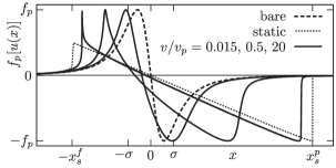
Figure 7: Velocity-dependence of the effective pinning force $f_{p}[u(x)]$ for a Lorentzian pin (with maximal force $f_{p}=2(3/8)^{3/2}e_{p}/\xi$) with Labusch parameter $\kappa=5$ and for velocities $v/v_{p}=0.015$, $0.5$, and $20$. The dynamical force profile is compared to the bare force $f_{p}(x)$ (dashed) and the static effective force $f_{p}[u_{s}(x)]$ (dotted). For small velocities, the finite-velocity solution follows closely the static solution $u_{s}(x)$, motivating an approximative scheme based on the latter as a starting point. For large velocities, the force profile approaches that of the bare force, motivating the use of perturbation theory around free flux flow.

The above results provide a good qualitative understanding of the velocity-dependence of the effective pinning force $f_{p}[u(x)]$ shown in Fig. 7 as calculated for a fixed Labusch parameter $\kappa=5$ and different velocities $v$. Indeed, one finds that at low and high velocities $v$, the effective dynamical force smoothly evolves out of the static force $f_{p}[u_{s}(x)]$ (dotted in Fig. 7) and the bare force $f_{p}(x)$ (dashed in Fig. 7). Furthermore, at intermediate velocities, the effective pinning force roughly follows a square-root shape of reduced extent, in agreement with the result (48). The average pinning force $\langle f_{p}(v)\rangle$ shown in Fig. 6 derives from an average over the local pinning force $f_{p}[u(x)]$, see Eq. (16). In the following, we present a more detailed analysis of the various pinning and velocity regimes.

IV.2 Perturbation theory around flux flow

When the effect of pinning is small, either at small $\kappa\ll 1$ or at high velocities $v$, we can use perturbation theory away from flux flow schmid_73 ; larkin_74 ; blatter_94 . This analysis can be done on the full two-dimensional problem at $z=0$, using the ansatz ${\bf u}({\bf R},t)={\bf v}t+{\bf u}_{p}({\bf R}+{\bf v}t)$ for the dynamical displacement field with the pinning contribution ${\bf u}_{p}$ providing a small correction. We start with Eq. (II) and expand the pinning force in ${\bf u}_{p}$ to obtain the correction

$$u_{p,\alpha}({\bf R}+{\bf v}t)\approx\int_{-\infty}^{t}dt^{\prime}G[0,(t-t^{\prime})]f_{p,\alpha}({\bf R}+{\bf v}t^{\prime}).$$ (49)

Next, we insert this expression back into the formula for the average pinning force density Eq. (11) (we assume a drive along $x$ with ${\bf v}=(v,0)$ and evaluate the average force at $t=0$) and arrive at

$$\langle F_{p}(v)\rangle \approx -n_{p}\int\frac{d^{2}R}{a_{0}^{2}}\,\partial_{\alpha}f_{p,x}({\bf R})$$

$$\qquad\qquad\quad\times\int_{0}^{\infty}dt\,G(0,t)\,f_{p,\alpha}({\bf R}-{\bf v}t).$$

This result can be brought to the form known from weak collective pinning theory,

$$\langle F_{p}(v)\rangle \approx \int_{0}^{\infty}dt\,G(0,t)\,K^{x\alpha\alpha}({\bf v}t)$$ (51)

with the pinning energy correlator

$$K({\bf u})=n_{p}\int\frac{d^{2}R}{a_{0}^{2}}\,e_{p}({\bf R})\,e_{p}({\bf R}-{\bf u})$$ (52)

and the superscripts in Eq. (51) denoting derivatives with respect to $u_{x}$ and $u_{\alpha}$ (and summation over $\alpha=x,y$). For weak pinning, the result Eq. (51) can be used for any velocity $v$.

IV.2.1 Weak pins, small $v$

We first show that the pinning force indeed increases $\propto\sqrt{v}$ at small velocities. This is easily done in Fourier space, which takes Eq. (51) into the form (we assume a drive along $x$)

$$\langle F_{p}(v)\rangle \approx \frac{n_{p}}{a_{0}^{2}}\int\frac{d^{2}K}{(2\pi)^{2}}\,K^{2}K_{x}\,|e_{p}({\bf K})|^{2}$$

$$\qquad\times\int_{0}^{\infty}\!\!dt\,G(0,t)\sin(K_{x}vt).$$

Using the 3D Green’s function Eq. (20) that is relevant at small velocities $v$, we obtain the result (with the numerical $\nu^{\scriptscriptstyle<}\approx K(1/2)/(3\sqrt{\pi}\pi^{2})$ and $K(m)$ the complete elliptic integral of the first kind)

$$\langle F_{p}(v)\rangle \approx \nu^{\scriptscriptstyle<}\frac{n_{p}}{a_{0}\lambda\bar{C}}\sqrt{\frac{v}{v_{\sigma}}}\int_{0}^{\infty}\!\!\!\!dK\,K^{4}\sqrt{K\sigma}|e_{p}(K)|^{2}$$ (54)

$$\sim \frac{\sigma^{2}}{a_{0}\lambda}n_{p}\kappa f_{p}\sqrt{\frac{v}{v_{\sigma}}},$$

where we provide a simple scaling estimate in the last line. Here, the velocity

$$v_{\sigma}=\sigma/t_{\mathrm{th}}$$ (55)

replaces $v_{p}$ at weak pinning $\kappa<1$. As expected, the average pinning force increases with velocity $v$ from zero with a dependence $\propto\sqrt{v/v_{\sigma}}$; this result can be traced back to the time dependence $\propto t^{-3/2}$ of the 3D Green’s function relevant at long times (and hence small velocities $v$) and a time integral that is cut on $t\sim 1/K_{x}v$.

The appearance of a finite pinning-force density for finite velocities $v$ is illustrated in Fig. 8. In the static situation, the pinning-force density $\langle F_{p}(v=0)\rangle=F_{c}$ vanishes for the single-valued anti-symmetric solution $u_{s}(x)=-u_{s}(-x)$ at weak pinning $\kappa\leq 1$. For finite velocities, the asymmetric deformation of the effective pinning force $f_{p}[u(x)]$ generates a finite positive result $\langle F_{p}(v)\rangle>0$ instead.

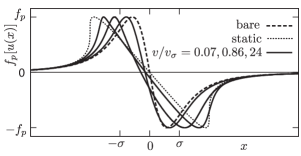
Figure 8: Velocity-dependence of the effective pinning force $f_{p}[u(x)]$ for a Lorentzian pin with Labusch parameter $\kappa=1.0$ and for velocities $v/v_{\sigma}=0.07$, $0.86$, and $24$. The dynamical force profile is compared to the bare force $f_{p}(x)$ (dashed) and the static effective force $f_{p}[u_{s}(x)]$ (dotted). The asymmetry in the effective pinning force $f_{p}[u(x)]$ (narrowing on the left as the vortex is dragged into the pin, broadening on the right as the vortex is held back in the pin) generates the finite pinning-force density $\langle F_{p}(v)\rangle$ at finite velocities, see Eq. (16).

The scaling $\propto\sqrt{v/v_{\sigma}}$ in the pinning-force density persists even beyond the Labusch point at $\kappa=1$, the only relevant change being the appearance of a finite critical force-density labusch_69 ; blatter_04 , $F_{c}\sim(\sigma x_{s}^{f}/a_{0}^{2})n_{p}f_{p}(\kappa-1)^{2}$, see Eq. (45), while the velocity dependent part $[\langle F_{p}(v)\rangle-F_{c}]\propto\sqrt{v/v_{\sigma}}$ evolves smoothly across the Labusch point.

Next, we remain in the weak pinning regime and follow the evolution of the average pinning-force density $\langle F_{p}(v)\rangle$ with increasing velocity. We use the perturbative result for the average pinning-force density Eq. (IV.2) in order to find a simple estimate for the evolution of $\langle F_{p}(v)\rangle$. The integration over space contributes a factor $\sigma^{2}$ due to the pin extension, the force derivative is estimated as $\partial_{x}f_{p}(x)\sim f_{p}/\sigma$, and the time integral over the Green’s function contributes a factor $tG(0,t)$; the conversion from time to velocity again involves the pin size $\sigma$, $v\sim\sigma/t$. Starting from small velocities $v$, we choose the appropriate Green’s function and obtain the results (with $\kappa<1$)

$$\langle F_{p}(v)\rangle \sim \frac{\sigma^{2}}{a_{0}^{2}}n_{p}\kappa f_{p}\left\{\begin{array}[]{ll}\displaystyle{\frac{a_{0}}{\lambda}\sqrt{\frac{v}{v_{\sigma}}},}&\displaystyle{\frac{v}{v_{\sigma}}<\frac{a_{0}^{2}}{\lambda^{2}},}\\ \vspace{3pt}\cr\displaystyle{\frac{v}{v_{\sigma}},}&\displaystyle{\frac{a_{0}^{2}}{\lambda^{2}}<\frac{v}{v_{\sigma}}<1,}\\ \vspace{3pt}\cr\displaystyle{\sqrt{\frac{v_{\sigma}}{v}},}&\displaystyle{1<\frac{v}{v_{\sigma}},}\\ \end{array}\right.$$ (59)

with a maximal pinning force $\sim(\sigma/a_{0})^{2}n_{p}\kappa f_{p}$ appearing at $v_{\sigma}$. For weak pinning, all these results remain within the perturbative regime with $|\delta u|<\sigma$. This is no longer true if we turn to very strong pinning with $\kappa\gg 1$.

IV.2.2 Very strong pins $\kappa\gg 1$, large $v>\kappa v_{p}$

For very strong pinning $\kappa\gg 1$, we have to make sure that the displacement $u_{p}$ remains small, $u_{p}<\sigma$. A simple estimate of Eq. (49) provides the high-velocity result (we consider short times and hence use the 1D Green’s function)

$$u_{p}(x)=\int_{0}^{\infty}dtG(0,t)f_{p}(x-vt)\sim\sigma\sqrt{\frac{\kappa v_{p}}{v}}.$$ (60)

Hence, for very strong pinning, perturbation theory becomes applicable only at very large velocities $v>\kappa v_{p}$. We can make use of Eq. (IV.2.1) and the 1D Green’s function Eq. (22) to find the high-velocity result (with the numerical $\nu^{\scriptscriptstyle>}\approx 2[\Gamma(3/4)]^{2}/(\sqrt{\pi}\pi^{2})$)

$$\langle F_{p}(v)\rangle \approx \nu^{\scriptscriptstyle>}\frac{n_{p}}{a_{0}^{2}\bar{C}}\sqrt{\frac{v_{\sigma}}{v}}\int_{0}^{\infty}\!\!\!\!dK\,(K^{4}/\sqrt{K\sigma})|e_{p}(K)|^{2}$$ (61)

$$\sim \frac{\sigma^{2}}{a_{0}^{2}}n_{p}f_{p}\sqrt{\frac{\kappa v_{p}}{v}}.$$

This result is consistent with a transverse trapping length $t_{\perp}\sim\sigma$, which is reduced by a factor $\kappa^{1/(n+2)}$ with respect to the static result of Eq. (33). As the velocity drops below $\kappa v_{p}$, new effects show up which require a self-consistent evaluation of the vortex dynamics—we will discuss this situation in Section IV.3 below.

IV.2.3 Weak collective- versus single pins

Before turning to the self-consistent dynamical solution, we comment on the relation between weak collective pinning theory and our single-pin approximation discussed above. The perturbative result Eq. (51) for the average pinning-force density $\langle F_{p}(v)\rangle$ obtained within our single-pin (SP) analysis coincides, to lowest order in $\kappa$ and in the pin density $n_{p}$, with the result obtained from weak collective pinning theory blatter_94 (WCP). On a first glance, this result may appear as a surprise, however, the correlations manifest in Eq. (51) arise quite naturally when constructing a pinning landscape with a finite density $n_{p}$ of randomly distributed pins of shape $\varepsilon_{p}({\bf r})$, see Eq. (4). The pinning energy density $E_{p}[{\bf r},{\bf u}]$ of such a disorder landscape can be written as

$$E_{p}[{\bf r},{\bf u}] = \sum_{\mu,i}e_{p}({\bf R}_{\mu}+{\bf u}_{\mu}(z)-{\bf R})\,\delta^{3}({\bf r}-{\bf r}_{i})$$ (62)

$$= \sum_{\mu}e_{p}({\bf R}_{\mu}+{\bf u}_{\mu}(z)-{\bf R})\,\rho_{p}({\bf r})$$

with the pin density

$$\rho_{p}({\bf r})=\sum_{i}\delta^{3}({\bf r}-{\bf r}_{i}).$$ (63)

The corresponding force field ${\bf F}_{p}[{\bf r},{\bf u}]$ relates to Eq. (5) via

$$\int\frac{d^{2}R}{a_{0}^{2}}{\bf F}_{p}[{\bf r},{\bf u}]=\sum_{\mu}{\bf F}_{p}({\bf r}_{\mu},{\bf u}_{\mu}).$$ (64)

Assuming self-averaging, the average pinning-force density $\langle{\bf F_{p}}\rangle$ in Eq. (5) then can be written as the volume average

$$\langle{\bf F_{p}}\rangle=-\frac{1}{V}\int d^{3}r\,{\bf F}_{p}[{\bf r},{\bf u}].$$ (65)

Rewriting ${\bf u}={\bf v}t+{\bf u}_{p}$ and expanding in ${\bf u}_{p}$ one obtains (for a drive along $x$)

$$\langle F_{p,x}\rangle = -\frac{1}{V}\!\int d^{3}r\!\int d^{3}r^{\prime}\!\int^{t}dt^{\prime}\,\partial_{\alpha}\partial_{x}E_{p}({\bf r},{\bf v}t)$$ (66)

$$\quad\times G_{\alpha\beta}({\bf r}-{\bf r}^{\prime},t-t^{\prime})\,\partial_{\beta}E_{p}({\bf r}^{\prime},{\bf v}t^{\prime}).$$

Inserting the form Eq. (62) of the pinning energy landscape and assuming small and weak pinning defects, the sums over pairs of vortices $\nu$ and $\mu$ and pairs of pins $i$ and $j$ reduce to those terms with $\mu=\nu$ and $i=j$; expressing the sums over vortices and pinning centers as integrals over $d^{2}R/a_{0}^{2}$ and $n_{p}d^{3}r_{p}$, we arrive at

$$\langle F_{p,x}\rangle = -n_{p}\int^{t}dt^{\prime}\,G(0,t-t^{\prime})$$

$$\qquad\times\int\frac{d^{2}R}{a_{0}^{2}}\,\partial_{\alpha}\partial_{x}e_{p}[{\bf R}+{\bf v}t]\,\partial_{\alpha}e_{p}[{\bf R}+{\bf v}t^{\prime}],$$

which, choosing the time $t=0$, is easily reduced to the result Eq. (51). Alternatively, one may take the average over disorder realizations on the right hand side of Eq. (66), represent the pinning energy density $E_{p}$ through Eq. (62), and use the density-density correlator

$$\langle\rho({\bf r})\rho({\bf r}^{\prime})\rangle=n_{p}^{2}+n_{p}\delta^{3}({\bf r}-{\bf r}^{\prime}).$$ (68)

The pinning energy correlator then is easily reduced to the usual form (the reducible term $n_{p}^{2}$ in Eq. (68) is irrelevant in the present discussion)

$$\langle E_{p}({\bf r},{\bf u})E_{p}({\bf r}^{\prime},{\bf u}^{\prime})\rangle=\delta^{3}({\bf r}-{\bf r}^{\prime})K({\bf u}-{\bf u}^{\prime})$$ (69)

with the $K({\bf u})$ given by Eq. (52) (again, we use that individual pins are small and weak, such that the sum over vortex pairs reduces to a single sum over $\mu=\nu$). Hence, the single-pin result Eq. (51) contains all the correlations present in the disorder landscape described by Eq. (62).

The single-pin approach predicts a vanishing critical force $F_{c}$ for $\kappa<1$, while the weak collective pinning scheme provides a finite result. This difference arises due to the different handling of the small velocity limit in the two approaches: In the weak pinning scenario, we stop decreasing the velocity $v$ when perturbation theory breaks down as the pinning-induced correction $\delta v$ becomes of order of the velocity $v$ itself; the criterion $\delta v\sim v\equiv v_{c}$ defines a finite (critical) pinning-force density $F_{c}^{\rm\scriptscriptstyle WCP}\equiv\langle F_{p}(v_{c})\rangle$. In the strong pinning scenario, instead, we take $v$ all the way to zero and obtain a vanishing critical force-density $F_{c}^{\rm\scriptscriptstyle SP}=0$. On the other hand, using the SP result Eq. (IV.2) and adopting the WCP cutoff scheme, we find a finite critical current density $j_{c}$ as well: with the estimate $\langle F_{p}(v)\rangle^{\rm\scriptscriptstyle SP}\sim n_{p}(\sigma/\lambda)(f_{p}^{2}/\varepsilon_{0})(v/v_{\sigma})^{1/2}$ from Eq. (59), valid at low velocities, and the conditions $\langle F_{p}(v_{c})\rangle^{\rm\scriptscriptstyle SP}\sim\eta v_{c}\sim j_{c}B/c$, we obtain the critical current density (with $j_{0}\sim c\varepsilon_{0}/\Phi_{0}\xi$ denoting the depairing current density and using $\sigma\sim\xi$)

$$j_{c}\sim j_{0}(\xi^{2}/\lambda^{2})\bigl{(}n_{p}a_{0}^{3}f_{p}^{2}/\varepsilon_{0}^{2}\bigr{)}^{2}\propto n_{p}^{2},$$ (70)

in agreement with the results obtained from weak collective pinning theory blatter_04 . This result is quite remarkable: first, the critical current (70) is proportional to $n_{p}^{2}$, the square of the pin density $n_{p}$, i.e., its origin is in the correlations between pins. Second, the result is still consistent with the standard SP result $\langle F_{p}(v=0)\rangle^{\rm\scriptscriptstyle SP}=0$, as the latter is an order $n_{p}$ result and corrections $\propto n_{p}^{2}$ are beyond the standard SP approach. For strong pinning $\kappa>1$, we already obtain a finite critical force $\langle F_{p}(v=0)\rangle^{\rm\scriptscriptstyle SP}\propto n_{p}$, linear in pin density. In this situation, pin-pin correlations are expected to provide corrections $o(n_{p})$ which vanish faster than linear, allowing us to approach the critical force parametrically closer than in the WCP situation.

IV.3 Universal self-consistent dynamical solution for very strong pins with $\kappa\gg 1$

Upon decreasing the velocity $v$ below $\kappa v_{p}$ in the very strong pinning regime, one has to account for the large deformation of the vortex before depinning. This is illustrated in Fig. 7, where the effective pinning force extends over a region $t_{\parallel}$ larger than $\sigma$ and reaches $x_{s}^{p}\sim\kappa\sigma$ at sufficiently low velocities. Here, we attempt to use Eq. (15) to find a self-consistent solution for the effective pinning force $f_{p}[u(x)]$ in the regime where the vortex deformation is still large.

In the very strong pinning regime and for velocities $v>v_{p}$ the largest time scale in the depinning process is given by $t\approx\kappa\sigma/v_{p}=t_{\mathrm{th}}$ and hence the relevant Green’s function entering Eq. (15) is given by the 1D expression Eq. (22). The self-consistency equation (15) then can be written as

$$u(x)-x = \frac{1}{\bar{C}\sqrt{vt_{\mathrm{th}}}}\int_{-\infty}^{x}dx^{\prime}\,\frac{f_{p}[u(x^{\prime})]}{\sqrt{x-x^{\prime}}}.$$ (71)

This equation can be solved in three regimes: i) For $x<-\sigma$, the vortex does not yet feel the pin and the equation is trivially solved by $u(x)=x$. ii) Similarly, for $x>t_{\parallel}$, the vortex has depinned and again $u(x)=x$. iii) In the intermediate region $-\sigma<x<t_{\parallel}\leq\kappa\sigma$, we make use of the Ansatz $f_{p}[u(x^{\prime})]=-\alpha f_{p}\sqrt{x^{\prime}+\sigma}$ (see also the discussion leading to Eq. (48) in Sec. IV.1 above) and find that

$$x-u(x) = \frac{\alpha\,f_{p}}{\bar{C}\sqrt{vt_{\mathrm{th}}}}\int_{-\sigma}^{x}dx^{\prime}\,\sqrt{(x^{\prime}+\sigma)/(x-x^{\prime})}$$

$$= \frac{\alpha\,\pi\,f_{p}}{2\bar{C}\sqrt{vt_{\mathrm{th}}}}(x+\sigma).$$

Dropping the small corrections $u(x)\lesssim\sigma\ll x$ on both sides of the equation, we find that the constant $\alpha=2\bar{C}\sqrt{vt_{\mathrm{th}}}/\pi f_{p}\approx 2\sqrt{vt_{\mathrm{th}}}/\pi\kappa\sigma$ provides a consistent solution, resulting in the dynamical effective pinning force

$$f_{p}[u(x\gg\sigma)] \approx -\frac{2}{\pi}\bar{C}\sqrt{vt_{\mathrm{th}}x}\sim-f_{p}\sqrt{\frac{v}{v_{p}}\frac{x}{\kappa\sigma}}.$$ (73)

At depinning, the force assumes its maximal value $-f_{p}$ and we find the longitudinal trapping length

$$t_{\parallel}(v>v_{p})\approx\frac{\pi^{2}}{4}\Bigl{(}\frac{f_{p}}{\bar{C}}\Bigr{)}^{2}\frac{1}{vt_{\mathrm{th}}}\sim\frac{v_{p}}{v}\kappa\sigma,$$ (74)

starting from $\sigma$ at high velocities $v\sim\kappa v_{p}$ and increasing to the maximal value $t_{\parallel}(v_{p})\sim\kappa\sigma$ as $v$ drops to $v_{p}$, see Sec. III. One easily checks that we indeed remain in the 1D elastic regime throughout this range of velocities: for velocities $v$ larger than $v_{p}$ one finds that the relevant time $t\sim t_{\parallel}(v)/v\sim t_{\mathrm{th}}(v_{p}/v)^{2}<t_{\mathrm{th}}$.

Combining Eqs. (73) and (74), we can provide a good approximation for the behavior of the dynamical effective pinning force at large values of $x\gg\sigma$,

$$f_{p}[u(x\gg\sigma)] \approx -f_{p}\sqrt{x/t_{\parallel}(v)}.$$ (75)

When the vortex depins at $t_{\parallel}(v)$, it attains its original straight shape back within a thermal time $t_{\mathrm{th}}$; this follows from the dissipative equation of motion for a vortex segment $a_{0}$ that is displaced by $u$, $\eta_{l}a_{0}u/t_{\mathrm{dp}}\sim\varepsilon_{0}u/a_{0}$ (with $\eta_{l}=\eta a_{0}^{2}$ the line friction), from which we obtain $t_{\mathrm{dp}}\sim\eta a_{0}^{4}/\varepsilon_{0}\sim t_{\mathrm{th}}$, see Eq. (19). During this depinning process, the vortex moves by a distance $x_{\mathrm{dp}}\sim vt_{\mathrm{th}}=\sigma v/v_{\sigma}$. As $v$ increases beyond $v_{\sigma}$, the depinning process smoothens, the depinning time is determined by the average motion, $t_{\mathrm{dp}}\sim\sigma/v$, and the depinning distance $x_{\mathrm{dp}}$ saturates at $\sigma$,

$$x_{\mathrm{dp}}(v) \sim \left\{\begin{array}[]{ll}\displaystyle{\sigma v/v_{\sigma},}&\displaystyle{v<v_{\sigma},}\\ \vspace{3pt}\cr\displaystyle{\sigma,}&\displaystyle{v_{\sigma}<v.}\\ \end{array}\right.$$ (78)

These results describe qualitatively well the depinning curves in Fig. 7.

Making use of the dynamical effective pinning force (73) in the expression for the average pinning force (14) and cutting the integral on $t_{\parallel}(v)$, we find that $\langle f_{p}(v)\rangle$ decays $\propto v_{p}/v$ over the extended velocity regime $v_{p}<v<\kappa v_{p}$,

$$\langle f_{p}(v)\rangle \approx \frac{\pi^{2}}{6}f_{p}\Bigl{(}\frac{f_{p}}{\bar{C}a_{0}}\Bigr{)}^{2}\frac{a_{0}}{vt_{\mathrm{th}}}\sim\frac{\kappa\sigma}{a_{0}}\frac{v_{p}}{v}f_{p},$$ (79)

where we have replaced $f_{p}/\bar{C}\sigma\approx\kappa$ in the second expression. The pinning-force density $\langle F_{p}(v)\rangle$ requires knowledge of the transverse pinning or trapping length $t_{\perp}(v)$ which will be calculated in Sec. IV.5.

IV.4 Perturbation theory around static solution

At low velocities, the dynamical force $f_{p}[u(x)]$ remains close to the static one $f_{p}[u_{s}(x)]$, as illustrated in the example of a Lorentzian potential shown in Fig. 7. The basic idea then is to construct a perturbative analysis away from the static solution $u_{s}(x)$; the latter rests on a reformulation of the dynamical equation (15) that makes use of the integrated Green’s function

$$G^{\uparrow}(x)=\int_{x}^{\infty}\frac{dx^{\prime}}{v}G(0,x^{\prime}/v)$$ (80)

and rewriting the Green’s function $G\bigl{[}(x-x^{\prime})/v\bigr{]}$ in Eq. (15) through the derivative $-v\partial_{x}G^{\uparrow}(x-x^{\prime})$. Interchanging the derivative and the integral, we can extract a term $f_{p}[u(x)]/\bar{C}$ and arrive at a formula reminiscent of the static variant (23),

$$u(x)=[x-\delta x[u](x)]+\frac{f_{p}[u(x)]}{\bar{C}},$$ (81)

with the coordinate shift

$$\delta x[u](x)=\partial_{x}\int_{-\infty}^{x}dx^{\prime}G^{\uparrow}(x-x^{\prime})f_{p}[u(x^{\prime})].$$ (82)

The dynamic solution $u(x)$ then can be expressedlarkin_86 through the smooth multi-valued static solution $\bar{u}_{s}(x)$ via the self-consistent coordinate shift $\delta x[u](x)$,

$$u(x)=\bar{u}_{s}\bigl{[}x-\delta x[u](x)\bigr{]}\equiv\bar{u}_{s}\bigl{[}x_{\mathrm{eff}}[u](x)\bigr{]}.$$ (83)

Here, the smooth static solution $\bar{u}_{s}(x)$ follows the free, unstable, and pinned branches and thus differs from $u_{s}(x)$ by a substitution of the jumps by the unstable branches. One easily checks that evaluating the static self-consistency equation (23) at $x-\delta x$ and making use of Eq. (83) reproduces the dynamical equation (81).

The integrated Green’s function (80) relevant in the coordinate shift $\delta x[u](x)$ assumes the form

$$G^{\uparrow}(x)\approx\left\{\begin{array}[]{ll}\displaystyle{\frac{1}{\bar{C}},}&\displaystyle{\frac{x}{vt_{\mathrm{th}}}<1,}\\ \vspace{3pt}\cr\displaystyle{\frac{1}{2\bar{C}}\frac{vt_{\mathrm{th}}}{x},}&\displaystyle{1<\frac{x}{vt_{\mathrm{th}}}<\frac{\lambda^{2}}{a_{0}^{2}},}\\ \vspace{3pt}\cr\displaystyle{\frac{1}{\pi}\frac{a_{0}}{\lambda}\frac{1}{\bar{C}}\sqrt{\frac{vt_{\mathrm{th}}}{x}},}&\displaystyle{\frac{\lambda^{2}}{a_{0}^{2}}<\frac{x}{vt_{\mathrm{th}}}.}\end{array}\right.$$ (87)

In the static limit $v\to 0$ the coordinate shift $\delta x[u](x)=0$ vanishes, except for two finite spikes of vanishing width $\propto\sqrt{v}$ at $-x_{s}^{f}$ and $x_{s}^{p}$, and the dynamic displacement approaches the static one, $u(x)\to u_{s}(x)$. Substantial changes in $\delta x[u](x)$ (and hence in $u(x)$ and $\langle f_{p}(v)\rangle$) are to be expected when the scale $vt_{\mathrm{th}}$ of $G^{\uparrow}(x)$ increases beyond the pinning scale $\kappa\sigma$ of $f_{p}[u(x)]$, confirming the estimate $v_{p}\sim\kappa\sigma/t_{\mathrm{th}}$ for the pinning velocity scale in Eq. (46).

Given the shape of the displacement $\bar{u}_{s}(x)$ as discussed above and illustrated in Fig. 3(a), let us first understand how this static solution generates the dynamic solution $u(x)$ via the coordinate shift $\delta x[u](x)$, see (83)—the precise understanding of this mapping is an important step in the construction of the perturbative analysis of the dynamical displacement $u(x)$ at small velocities $v$ discussed below.

The most noticeable feature in the static solution ${u}_{s}(x)$ are the jumps at $-x_{s}^{f}$ and $x_{s}^{p}$ marking the trapping of the vortex tip and its depinning. These jumps imply that the vortex does not probe all of the pin potential. In the dynamic situation, the vortex tip moves with a finite velocity across the pin and thus has to pass every point in the pinning potential at some time, hence the dynamical solution $u(x)$ has to be continuous in $x$. The relation (83) maps the continuous function $u(x)$ via the shift function $\delta x[u](x)$ to the static solution $\bar{u}_{s}(x)$ of Eq. (23), where $u(x)$ probes all three branches of the static solution $\bar{u}_{s}(x)$, free, unstable, and pinned ones. In order to do so, the shift $\delta x[u](x)$ or the effective coordinate $x_{\mathrm{eff}}[u](x)=x-\delta x[u](x)$ has to develop (sharp) negative spikes close to the points $-x_{s}^{f}$ and $x_{s}^{p}$, see Fig. 3(b). These spikes start at the shifted positions $-x^{f}$ and $x^{p}$ defined through the conditions $-x^{f}-\delta x[u](-x^{f})=x_{\mathrm{eff}}[u](-x^{f})=-x_{s}^{f}$ and $x^{p}-\delta x[u](x^{p})=x_{\mathrm{eff}}[u](x^{p})=x_{s}^{p}$ (note that $u(-x^{f})=u_{s}(-x_{s}^{f})$ and $u(x^{p})=u_{s}(x_{s}^{p})$, see Figs. 3(a) and (b)). The height of these spikes are such as to shift the unstable branches $u_{s}^{u}(x)$ to the dynamical solution $u(x)$ (dotted arrows in Fig. 3(a)). It turns out, that the shift function $\delta x[u](x)$ is the central quantity in the perturbative calculation of $\langle f_{p}(v)\rangle$.

IV.4.1 Very strong pinning with $\kappa\gg 1$

Our goal is to find the correction in the average pinning force

$$\langle f_{p}(v)\rangle-f_{c} \equiv \langle\delta f_{p}(v)\rangle$$

$$= -\frac{1}{a_{0}}\int_{-\infty}^{\infty}\!\!\!\!dx\,\bigl{(}f_{p}[u(x)]-f_{p}[u_{s}(x)]\bigr{)}.$$

The difficulties with the evaluation of Eq. (IV.4.1) are the steep slopes in $u(x)$ and jumps in $u_{s}(x)$ when the vortex enters and leaves the pin, see Fig. 3. While the jumps in $u_{s}(x)$ appear at the positions $-x_{s}^{f}$ and $x_{s}^{p}$, these positions are shifted to $-x^{f}$ and $x_{p}$ for the dynamical solution $u(x)$. The shifted positions are easily obtained from Eq. (83): The dynamical solution $u(x)$ leaves the free (pinned) branch of $u_{s}(x)$ when $x-\delta x[u](x)$ coincides with $-x_{s}^{f}$ ($x_{s}^{p}$), hence

$$-x^{f}-\delta x[u](-x^{f}) = -x_{s}^{f},$$ (89)

$$x^{p}-\delta x[u](x^{p}) = x_{s}^{p}.$$ (90)

At the locations $-x_{s}^{f}$, $-x^{f}$, $x^{p}$, and $x_{s}^{p}$ either the static ($f_{p}[u_{s}(x)]$) or dynamic ($f_{p}[u(x)]$) force changes rapidly between free and pinned branches. We then can split the integral in Eq. (IV.4.1) into appropriate intervals with and without jumps,

$$\langle\delta f_{p}(v)\rangle=-\frac{1}{a_{0}}\biggl{[}\int_{-\infty}^{-x_{s}^{f}}\!\!\!\!\!\!\!\!dx\,\delta f_{ff}(x)+\int_{-x_{s}^{f}}^{-x^{f}}\!\!\!\!\!\!\!\!dx\,\delta f_{fp}(x)$$ (91)

$$+\int_{-x^{f}}^{x^{p}}\!\!\!\!\!dx\,\delta f_{pp}(x)+\int_{x^{p}}^{x_{s}^{p}}\!\!\!\!dx\,\delta f_{fp}(x)+\int_{x_{s}^{p}}^{\infty}\!\!\!\!dx\,\delta f_{ff}(x)\biggr{]},$$

where

$$\delta f_{ab}(x)\equiv f_{p}[u_{s}^{a}(x-\delta x[u](x))]-f_{p}[u_{s}^{b}(x)]$$ (92)

and $u_{s}^{a}$ with $a\in\{f,p\}$ denote free and pinned branches of the static solution $u_{s}(x)$ (we have expressed $u(x)$ through Eq. (83) but do not resolve the steep rise in $u(x)$ on the unstable branch). Out of the five terms in Eq. (91), we can drop the first and last integrals: For a compact pin, the force is small, of order $f_{p}/\kappa$ just before $-x_{s}^{f}$ and negligible on the free branch at $x_{s}^{p}$, see the discussion in Sec. III.3 above. The first integral then is small by the factor $\kappa^{-3/2}$ as compared to the main terms, while the last integral is exponentially small. For a Lorentzian pin with large tails, the force is of order $f_{p}/\kappa^{3/4}$ at $-x_{s}^{f}$; it contributes a term smaller by $\kappa^{-9/8}$ as compared to the leading terms. In the last integral, the force starts at a value of order $-f_{p}/\kappa^{3}$ and its contribution is small by the factor $\kappa^{-6}$.

The second term describes the part of the jump into the pin when the dynamic solution has not yet responded to the presence of the pin, while the static solution has already jumped. This term scales the same way as the first integral: for a compact pin of size $\sigma$, the pinning force $f_{p}/\kappa$ is still small and the term is small by a factor $\kappa^{-3/2}$, while for a Lorentzian pin its contribution is small by the factor $\kappa^{-9/8}$ and can be safely ignored as well.

The important terms are the third and fourth ones describing the change in the pinning force as the vortex moves through the pin and the force difference arising from the substantial change in the location of depinning, respectively,

$$\langle\delta f_{p}(v)\rangle\approx-\frac{1}{a_{0}}\biggl{[}\int_{-x^{f}}^{x^{p}}\!\!\!\!\!\!\!\!dx\,\delta f_{pp}(x)+\!\!\int_{x^{p}}^{x_{s}^{p}}\!\!\!\!\!\!\!dx\,\delta f_{fp}(x)\biggr{]}.$$ (93)

In order to analyze this expression further, we have to investigate the behavior of the coordinate shift $\delta x[u](x)$, see Eq. (82). This shift is small, $\propto\sqrt{v}$, over most of the pinning interval $[-x^{f},x^{p}]$, where the (small) velocity parameter arises from the integrated Green’s function $G^{\uparrow}(x=vt)$, see the third line of Eq. (87). A notable exception are the two spikes at $-x^{f}$ and at $x^{p}$ where the vortex jumps into and out of the pin. These spikes are large, of size $x_{s}^{p}-x_{s}^{f}\sim\sigma\kappa$, but extend only over a small interval $\sim vt_{\mathrm{th}}$, see (78).

Away from these spikes, we can approximate the coordinate shift $\delta x[u](x)$ by $\delta x[u_{s}](x)$. In fact, the difference $\delta x[u](x)-\delta x[u_{s}](x)$ involves the force difference $f_{p}[u(x)]-f_{p}[u_{s}(x)]$ as it appears in the correction $\langle\delta f_{p}(v)\rangle$ given by Eq. (IV.4.1) above, multiplied with the Green’s function $G^{\uparrow}(x)\propto\sqrt{v/v_{\sigma}}$, see Eq. (87). Taking the coordinate $x$ through the various regimes, one can show that $\delta x[u](x)\approx\delta x[u_{s}](x)$ to order $v$ away from the jumps (with one factor $\sqrt{v}$ originating from the force difference and another from the Green’s function $G^{\uparrow}$) and to order $\sqrt{v}$ in a region of order $\sqrt{v}$ near the jumps (we ignore the region of size $vt_{\mathrm{th}}$ at the jumps where the difference is of order $\sigma\kappa$). Furthermore, we can replace (to precision $\sqrt{v}$) the positions $-x^{f}$ and $x^{p}$ by their static counterparts,

$$x_{s}^{f}-x^{f} = \delta x[u](-x^{f})\approx\delta x[u^{f}_{s}](-x_{s}^{f})\propto\sqrt{v},$$ (94)

and similarly (note that we have to make sure that we always stay on well-defined, continuous branches)

$$x_{s}^{p}-x^{p} = -\delta x[u](x^{p})\approx-\delta x[u^{p}_{s}](x_{s}^{p})\propto\sqrt{v}.$$ (95)

In simplifying Eq. (93), we make use of the smallness of $\delta x[u](x)$ in the interval $[-x^{f},x^{p}]$ and expand the integrand $\delta f_{pp}(x)\approx\partial_{x}f_{p}[u^{p}_{s}(x)]\,\delta x[u](x)$. Next, we replace (to lowest order in $v$) the unknown dynamical quantities $u(x)$, $x^{f}$, and $x^{p}$ by the known static expressions $u_{s}(x)$, $x_{s}^{f}$, and $x_{s}^{p}$. Finally, we replace the second integral by the product of force difference $\delta f_{fp}(x)\approx f_{p}[u_{s}^{f}(x_{s}^{p})]-f_{p}[u_{s}^{p}(x_{s}^{p})]$ times the width $x_{s}^{p}-x^{p}\approx-\delta x[u_{s}^{p}](x_{s}^{p})$ of the integration region, exploiting the sharp decay of both $f_{p}[u_{s}(x)]$ and $f_{p}[u(x)]$ at the boundaries. While the former is a property of the static solution, that latter is guaranteed by the smallness of the depinning length $x_{\mathrm{dp}}\propto v$, see Eq. (78). We then arrive at the closed expression for the average pinning force that contains only the static solution $u_{s}(x)$,

$$\langle\delta f_{p}(v)\rangle \approx \frac{1}{a_{0}}\biggl{[}\int_{-x_{s}^{f}}^{x_{s}^{p}}\!\!\!\!\!\!\!dx\,\partial_{x}f_{p}[u_{s}^{p}(x)]\,\delta x[u_{s}^{p}](x)$$

$$+\,\delta x[u_{s}^{p}](x_{s}^{p})\,\bigl{\{}f_{p}[u_{s}^{f}(x_{s}^{p})]-f_{p}[u_{s}^{p}(x_{s}^{p})]\bigr{\}}\biggr{]}.$$

An equivalent formula was obtained by Larkin and Ovchinnikov in Ref. [larkin_86, ] for a periodic pinning model describing large defects; the regularization introduced in their analysis follows from our derivation.

Making use of the universal solution for the static strong pinning force in Sec. III.3, we can find the sign of the small-velocity behavior of $\langle\delta f_{p}(v)\rangle$. We replace the force gradient by the (negative) effective elasticity $-\bar{C}\approx-f_{p}/\kappa\sigma$ in the first term and set the forces to zero and to $-f_{p}$ on the free and pinned branches in the second term to arrive at

$$\langle\delta f_{p}(v)\rangle \approx -\frac{f_{p}}{a_{0}}\biggl{[}\int_{-x_{s}^{f}}^{x_{s}^{p}}\!\!\!\!\!\!\!\!dx\frac{\delta x[u_{s}^{p}](x)}{\kappa\sigma}\!-\!\delta x[u_{s}^{p}](x_{s}^{p})\biggr{]}$$ (97)

$$= -\frac{f_{p}}{a_{0}}\bigl{[}\overline{\delta x[u_{s}^{p}](x)}-\delta x[u_{s}^{p}](x_{s}^{p})\bigr{]},$$

where $\>\overline{\cdots}\>$ denotes the average over the interval $[-x_{s}^{f},x_{s}^{p}]$. Finally, we use again the linear form $-\bar{C}x$ for the effective pinning force and the expression (87), $G^{\uparrow}\propto 1/\sqrt{x}$ (valid in the limit $v\to 0$) for the integrated Green’s function, in the calculation of the coordinate shift $\delta x[u_{s}^{p}](x)$,

$$\delta x[u_{s}^{p}](x) \approx -\bar{C}\partial_{x}\int_{0}^{x}dx^{\prime}G^{\uparrow}(x-x^{\prime})\,x^{\prime}$$ (98)

$$\sim -\sigma\frac{a_{0}}{\lambda}\sqrt{\frac{v\,x}{v_{\sigma}\,\sigma}}.$$

Here, we have ignored the part of $\delta x$ describing the jump into the pin by starting the integration from $x=0$. Making use of Eq. (98) in (97), the dynamical pinning force correction then assumes a negative value

$$\langle\delta f_{p}(v)\rangle\sim-\frac{a_{0}}{\lambda}f_{c}\sqrt{\frac{v}{v_{p}}}.$$ (99)

This negative correction can be easily understood by noting that $-\delta x[u_{s}^{p}](x)$ is a monotonically increasing positive function and hence the second (boundary) term in (97) always dominates over the average defining the first term.

The above result applies to the very strong pinning situation with $\kappa\gg 1$. On the other hand, we have seen in Sec. IV.2.1 that the pinning-force density is positive, $\langle F_{p}(v)\rangle\propto\sqrt{v/v_{\sigma}}$ when pinning is weak and $F_{c}=0$. The question arises about the origin of the sign change in $\langle\delta f_{p}(v)\rangle$ and for which value of $\kappa$ this sign change occurs.

IV.4.2 Moderately strong pinning with $\kappa\gtrsim 1$

In order to understand the sign change in $\langle\delta f_{p}(v)\rangle$, we have to be more accurate in our description of $f_{p}[u_{s}^{p}(x)]$ near depinning at $x_{s}^{p}$, as it is the last term in Eq. (97) that is strongly modified when $\kappa$ decreases, while the first term remains unchanged. Indeed, as $\kappa$ decreases, the decrease $f_{p}/2\kappa^{2}$ in the magnitude of $f_{p}[u_{s}^{p}(x)]$ before the jump at $x_{s}^{p}$ increases, see Eq. (44), leaving a smaller jump at $x_{s}^{p}$. Furthermore, the coordinate shift $\delta x[u_{s}^{p}](x)$ starts decreasing before the jump such that $x_{s}^{p}-x^{p}$ becomes small. These modifications lead to a reduction of the second term in Eq. (97), which is nothing but the signature of a decreasing critical force average $f_{c}$.

More precisely, we can use the result Eq. (44) for the static pinning force $f_{p}[u_{s}(x)]=f_{p}[u_{s}^{p}(x)]$ to obtain a more accurate expression for the coordinate shift. We make use of the expression (87) for the integrated Green’s function, $G^{\uparrow}(x-x^{\prime})\propto\sqrt{vt_{\mathrm{th}}/(x-x^{\prime})}$ for $x-x^{\prime}>vt_{\mathrm{th}}$, cut the integral at $x^{\prime}=x-vt_{\mathrm{th}}$, and concentrate on the leading terms which are large close to $x\approx x_{s}^{p}$ to obtain

$$\delta x[u](x)\approx\delta x[u_{s}^{p}](x)$$ (100)

$$\qquad\qquad\approx\frac{\partial}{\partial x}\int_{-\infty}^{x}\!\!\!\!\!dx^{\prime}G^{\uparrow}(x-x^{\prime})\,f_{p}[u_{s}^{p}(x^{\prime})]$$

$$\quad\approx-\frac{\sigma}{\pi}\frac{a_{0}}{\lambda}\sqrt{\frac{v}{v_{\sigma}}}\biggl{[}2\sqrt{\frac{x}{\sigma}}-\sqrt{\frac{\sigma\bar{C}}{2f_{p}}}\ln\frac{\sqrt{x_{s}^{p}}+\sqrt{x}}{\sqrt{x_{s}^{p}}\!-\!\sqrt{x-vt_{\mathrm{th}}}}\biggr{]}.$$

As expected, the coordinate shift is small in $\sqrt{v}$ and increases in magnitude $\propto\sqrt{x}$, see Eq. (98). However, due to the decrease in the magnitude of the pinning force on approaching $x_{s}^{p}$, a logarithmic correction appears, leading to a sharp collapse of $\delta x$ at $x_{s}^{p}$ which is cutoff (due to the transition to the single-vortex response) by the term $vt_{\mathrm{th}}$. Inserting the result (100) into the expression (97), we find that the velocity correction to the average pinning force assumes the form

$$\langle\delta f_{p}(v)\rangle \approx \frac{(x_{s}^{p}+x_{s}^{f})}{\pi\lambda}f_{p}\sqrt{\frac{vt_{\mathrm{th}}}{x_{s}^{p}+x_{s}^{f}}}$$ (101)

$$\qquad\qquad\qquad\times\Bigl{[}-\frac{2}{3}+\frac{1}{4\sqrt{2}}\frac{\sigma\bar{C}}{f_{p}}\ln\frac{4v_{p}}{v}\Bigr{]},$$

$$\sim \frac{\kappa\sigma}{\lambda}f_{p}\sqrt{\frac{v}{v_{p}}}\Bigl{[}-\frac{2}{3}+\frac{1}{4\sqrt{2}}\frac{\sigma\bar{C}}{f_{p}}\ln\frac{4v_{p}}{v}\Bigr{]}.$$

This more accurate analysis shows that $\langle\delta f_{p}(v)\rangle$ always increases with $v$ at very small velocities $v$, however, the corresponding velocity range is exponentially small in $\kappa\sim f_{p}/\sigma\bar{C}$, $v<v_{p}\exp(-\nu\kappa)$ with $\nu=(2\sqrt{2}/3)4\approx 4$, and therefore irrelevant at very strong pinning with $\kappa\gg 1$. Indeed, the small upturn predicted by Eq. (101) is not visible in Fig. 6. The result Eq. (101) straightforwardly provides the pinning-force density $\langle F_{p}(v)\rangle$ when combined with the result for the transverse trapping length $t_{\perp}(v)$ derived in the next section.

IV.5 Dynamical transverse trapping length $t_{\perp}$

The transverse trapping length $t_{\perp}$ has been found for the two limits of static pinning at vanishing velocity $v=0$ and in the perturbative high-velocity regime $v>\kappa v_{p}$. The static limit has been discussed in Sec. III.2, providing us with the result $t_{\perp}=R_{s}^{f}$, the asymptotic position where the free-branch minimum of the total pinning energy $e_{t}(R;r)$ in Eq. (31) vanishes; for a very strong pin with tails, $R_{s}^{f}\sim\sigma\kappa^{1/(n+2)}$. This result is parametrically larger than the one we found at very large velocities $v>\kappa v_{p}$ using perturbation theory where $t_{\perp}\sim\sigma$, see Sec. IV.2.2. The question then poses itself, how the transverse trapping length shrinks from $t_{\perp}\sim\sigma\kappa^{1/(n+2)}$ to $t_{\perp}\sim\sigma$ as the velocity $v$ increases.

We start from the static situation and consider the spherically symmetric total energy of Eq. (31) at the critical radius $R_{s}^{f}$ where the first and second derivative vanish, $\partial_{r}e_{t}(R;r)|_{R_{s}^{f},r_{s}^{f}}=0$ and $\partial_{r}^{2}e_{t}(R;r)|_{R_{s}^{f},r_{s}^{f}}=0$, and the free branch disappears. We consider the limit of very strong pinning (otherwise $t_{\perp}\sim\sigma$ follows trivially) and assume a pinning potential with long tails, $e_{p}(r)\sim-e_{p}\,(\sigma/r)^{n}$, $n=2$ for a Lorentzian shape defect potential. The critical asymptotic ($R_{s}^{f}$) and tip ($r_{s}^{f}<R_{s}^{f}$) positions where the free branch terminates then can be estimated to be located at the radii $R_{s}^{f}\gtrsim r_{s}^{f}\sim\sigma\kappa^{1/(n+2)}$, where we have dropped numericals and set $\kappa\sim e_{p}/\sigma^{2}\bar{C}$. The expansion of the total potential at $R_{s}^{f}$ in the vicinity of $r_{s}^{f}$ then is given by the cubic parabola (we drop a constant of order $\bar{C}\,(r_{s}^{f})^{2}$)

$$e_{t}(R_{s}^{f};r)=\alpha(r-r_{s}^{f})^{3},\quad\alpha\sim\frac{\bar{C}}{r_{s}^{f}f}.$$ (102)

The vortex tip (in the form of a segment of length $a_{0}$) then follows the equation of motion $\eta_{l}a_{0}\,\dot{r}=-\partial_{r}e_{t}=-\alpha(r-r_{s}^{f})^{2}$; in the static limit, every vortex approaching the defect with an impact parameter $b<R_{s}^{f}$ will fall to the center, having an infinity of time available to overcome the flat potential around $r_{s}^{f}$. In the dynamical situation, the vortex passes the pin with a finite velocity $v$ and we have to include an additional force-term $-\bar{C}[R_{s}^{f}-R(t)]$ in the equation of motion; here, ${\bf R}(t)=(-X^{f}+vt,Y^{f})$ denotes the moving asymptotic position of the vortex entering the critical radius $R_{s}^{f}$ around the defect at $t=0$ from the left. Assuming an impact parameter $b$ close to $R_{s}^{f}$, we can expand $R(t)\approx R^{f}(1-X_{s}^{f}vt/(R_{s}^{f})^{2})$, where we follow the trajectory over a time $t\leq X_{s}^{f}/v\equiv t_{\mathrm{tra}}$ to $X=0$, half the time to traverse the defect potential. The equation of motion

$$\eta_{l}a_{0}\,\dot{r}=-\alpha(r-r_{s}^{f})^{2}-\bar{C}(X_{s}^{f}/R_{s}^{f})vt$$ (103)

then picks up an additional force-term that is linear in time $t$ and independent on position $r$. Therefore, equation (103) can be brought to the form of Riccati’s equationBenderOrszag , $\dot{\bar{r}}={\bar{r}}^{2}+\bar{t}$, where we have introduced the dimensionless variables $\bar{r}$ and $\bar{t}$ via $r=r_{s}^{f}(1-\beta^{1/3}\bar{r})$ and $t=t_{\mathrm{th}}\beta^{-1/3}\bar{t}$ with $\beta=(X_{s}^{f}/R_{s}^{f})\,vt_{\mathrm{th}}/r_{s}^{f}$. Starting from $\bar{r}(\bar{t}=0)=0$, the radius $\bar{r}$ starts out small and we can drop the $\bar{r}^{2}$ term to find the solution $\bar{r}(\bar{t}\,)\approx\bar{t}^{\,2}/2$. When $\bar{r}$ is large, we can drop the $\bar{t}$ term and obtain the solution $\bar{r}(\bar{t}\,)\approx 1/(\bar{t}^{*}-\bar{t})$ with $\bar{t}^{*}$ an integration constant of order unity. In order to find the precise location of the divergence, one has to perform a numerical integration that provides the result $\bar{t}^{*}\approx 1.986$, see Ref. [BenderOrszag, ]. Thus, as a result, we find that the vortex tip falls to the center within the time window (we use $\bar{t}^{*}\approx 2$)

$$t_{\mathrm{fall}}\lesssim 2t_{\mathrm{th}}\Bigl{(}\frac{r_{s}^{f}R_{s}^{f}}{X_{s}^{f}\,vt_{\mathrm{th}}}\Bigr{)}^{1/3}.$$ (104)

The vortex tip has to fall to the center within a time smaller than $t_{\mathrm{tra}}\approx X_{s}^{f}/v$, from which we find the condition $(X_{s}^{f})^{2}\gtrsim R_{s}^{f}\,vt_{\mathrm{th}}$ (we approximate $r_{s}^{f}\approx R_{s}^{f}$). We thus obtain an upper limit on the impact parameter $b=[(R_{s}^{f})^{2}-(X_{s}^{f})^{2}]^{1/2}$ of vortices that can be trapped, what provides us with a result for the transverse trapping length $t_{\perp}(v)$ at small velocities,

$$R_{s}^{f}-t_{\perp}(v)\sim\frac{vt_{\mathrm{th}}}{R_{s}^{f}}.$$ (105)

The above analysis applies to impact parameters $b$ close to $R_{s}^{f}$ (or small $X_{s}^{f}$) where the tip trajectory is dominated by the slow motion near $r_{s}^{f}$. At small impact parameters $b$ of order a fraction of $R_{s}^{f}$, the elastic term in $e_{t}$ is no longer relevant and we have to consider the motion of the vortex tip in the radial pinning potential $e_{p}(r)$. The equation of motion then has to be replaced by $\eta_{l}a_{0}\,\dot{r}\sim-f_{p}(\sigma/r)^{n+1}$ and its integration leads to the trajectory

$$r(t)=r_{0}\bigl{(}1-t/t_{\mathrm{fall}}\bigr{)}^{\!1/(n+2)}\!\!,\quad t_{\mathrm{fall}}\sim t_{\mathrm{th}}\Bigl{(}\frac{r_{0}}{R_{s}^{f}}\Bigr{)}^{\!n+2},$$ (106)

where $r_{0}$ denotes the starting radius at $t=0$. The fastest fall to the center appears at the closest approach to the defect and hence we choose $r_{0}\sim b$. Again, the time to fall to the center has to be smaller than the traversing time which we estimate as $t_{\mathrm{tra}}\sim b/v$ as given by the geometry of the problem. As a result, we find that trajectories with an impact parameter

$$b<t_{\perp}(v)\sim R_{s}^{f}\Bigl{(}\frac{R_{s}^{f}}{vt_{\mathrm{th}}}\Bigr{)}^{1/(n+1)}$$ (107)

fall into the pin. The above result applies for velocities such that $t_{\perp}\gtrsim\sigma$, i.e., for $v>v_{p}$.

Combining the results (105) and (107), we find that the trapping length $t_{\perp}(v)$ decreases with increasing velocity $v$ on the velocity scale $R_{s}^{f}/t_{\mathrm{th}}\sim v_{p}/\kappa^{(n+1)/(n+2)}$, first with a correction factor $\propto 1-\kappa^{(n+1)/(n+2)}v/v_{p}$ and then with a power law $\propto[v_{p}/(\kappa^{(n+1)/(n+2)}v)]^{1/(n+1)}$. Hence, the transverse length $t_{\perp}(v)$ decreases from $R_{s}^{f}$ at $v=0$ to $\sigma$ at a velocity $v_{p}$.

The two trapping lengths $t_{\perp}(v)$ and $t_{\parallel}(v)$, see Eq. (74), define the trapping area $S_{\mathrm{trap}}(v)=2t_{\perp}(v)t_{\parallel}(v)$ which decreases smoothly from $S_{\mathrm{trap}}\sim\kappa^{(n+3)/(n+2)}\sigma^{2}$ at $v=0$ to $S_{\mathrm{trap}}\sim\sigma^{2}$ at $v\sim\kappa v_{p}$ and remains constant thereafter. Within the region $0<v<v_{p}$, this decrease is due to the reduction of $t_{\perp}$ from $\kappa^{1/(n+2)}\sigma$ to $\sigma$, while for velocities $v_{p}<v<\kappa v_{p}$ it is the longitudinal length $t_{\parallel}$ that shrinks from $\kappa\sigma$ to $\sigma$.

We note that the velocity scale $v_{\sigma}\kappa^{1/(n+2)}$ can also been obtained from a perturbative analysis: for a vortex with asymptotic position $-x<0$ passing the pin’s center at $t=0$, the pinning-induced correction (49) can be estimated as

$$u_{p}\sim\frac{\kappa\sigma^{n+2}}{t_{\mathrm{th}}} \biggl{[}\displaystyle{\int_{0}^{t_{\mathrm{th}}}\!\!\!\!dt\Bigl{(}\frac{t_{\mathrm{th}}}{t}\Bigr{)}^{1/2}\!\!+\!\!\int_{t_{\mathrm{th}}}^{\infty}\!\!\!\!dt\Bigl{(}\frac{t_{\mathrm{th}}}{t}\Bigr{)}^{3/2}\biggr{]}}$$

$$\times\displaystyle{\frac{x+vt}{[\sigma^{2}+(x+vt)^{2}]^{(n+2)/2}}}.$$

For small velocities $v<x/t_{\mathrm{th}}$, the integral assumes its main contribution from $t\sim t_{\mathrm{th}}$ and we find that $u_{p}\sim\kappa\sigma\,(\sigma/x)^{n+1}$, while for larger velocities the integral is cut at $v/x$ and $u_{p}\sim\kappa\sigma\,(\sigma/x)^{n+1}(x/vt_{\mathrm{th}})^{1/2}$. The perturbation theory breaks down when $u_{p}\sim x$, i.e., at the distance $x_{s}^{f}$ at small velocities and at $x_{s}^{f}\,(v_{\sigma}\kappa^{1/(n+2)}/v)^{1/2(n+3/2)}$ at high velocities, implying a reduction of the large-distance perturbative region on the velocity scale $v_{\sigma}\kappa^{1/(n+2)}$.

IV.6 Summary of force densities

We conclude this section with a summary of results for the dynamic pinning force density $\langle F_{p}(v)\rangle(=F_{c}+\langle\delta F_{p}(v)\rangle)$ on the level of dimensional estimates. For small and intermediate velocities $v<\kappa v_{p}$, more accurate expressions are obtained by combining the results for the average pinning force $\langle f_{p}(v)\rangle$, Eqs. (30), (79), and (101), with those for the transverse trapping length $t_{\perp}(v)$, Eqs. (105) and (107), and using Eq. (16). At high velocities $v>\kappa v_{p}$, the perturbative result Eq. (61) for $\langle F_{p}(v)\rangle$ can be used.

Starting out at $v=0$, we have the critical force-density

$$F_{c}\sim\frac{\kappa\sigma x_{s}^{f}}{a_{0}^{2}}n_{p}f_{p}\frac{(\kappa-1)^{2}}{\kappa^{2}}$$ (109)

in a form that is valid for all values $\kappa\geq 1$. The corrections at small velocities $v<v_{p}$ are given by $\langle\delta F_{p}(v)\rangle=(2t_{\perp}(v)/a_{0})n_{p}\langle\delta f_{p}(v)\rangle$ with

$$\langle\delta f_{p}(v)\rangle \sim \left\{\begin{array}[]{ll}\displaystyle{-\frac{\kappa\sigma}{\lambda}f_{p}\Bigl{(}\frac{v}{v_{p}}\Bigr{)}^{\!\frac{1}{2}},}&\displaystyle{\frac{v}{v_{p}}<\frac{a_{0}^{2}}{\lambda^{2}},}\\ \vspace{5pt}\cr\displaystyle{-\frac{\kappa\sigma}{a_{0}}f_{p}\frac{v}{v_{p}},}&\displaystyle{\frac{a_{0}^{2}}{\lambda^{2}}<\frac{v}{v_{p}}<1,}\end{array}\right.$$ (112)

and

$$t_{\perp}(v) \sim \left\{\begin{array}[]{ll}\displaystyle{x_{s}^{f}\Bigl{(}1-\frac{v\kappa^{\frac{n+1}{n+2}}}{v_{p}}\Bigr{)},}&\displaystyle{\frac{v}{v_{p}}\ll\kappa^{-\frac{n+1}{n+2}},}\\ \vspace{5pt}\cr\displaystyle{x_{s}^{f}\Bigl{(}\frac{v_{p}}{v\kappa^{\frac{n+1}{n+2}}}\Bigr{)}^{\frac{1}{n+1}}\!\!,}&\displaystyle{\kappa^{-\frac{n+1}{n+2}}<\frac{v}{v_{p}}<1,}\\ \vspace{5pt}\cr\displaystyle{\sigma,}&\displaystyle{1<\frac{v}{v_{p}}.}\end{array}\right.$$ (116)

The corresponding results for moderate values of $\kappa$ remain unchanged up to a sign change in $\langle\delta f_{p}(v)\rangle$, i.e., $\langle f_{p}(v)\rangle$ increases with $v$. Increasing the velocity beyond $v_{p}$, we have the following results for the pinning-force density $\langle F_{p}(v)\rangle$, see Eqs. (79) and (61),

$$\langle F_{p}(v)\rangle\sim\frac{\kappa\sigma^{2}}{a_{0}^{2}}n_{p}f_{p}\left\{\begin{array}[]{ll}\displaystyle{\frac{v_{p}}{v},}&\quad\displaystyle{1<\frac{v}{v_{p}}<\kappa,}\\ \vspace{3pt}\cr\displaystyle{\sqrt{\frac{v_{p}}{\kappa v}},}&\quad\displaystyle{\kappa<\frac{v}{v_{p}}.}\\ \end{array}\right.$$ (119)

Again, these results remain valid as $\kappa$ is reduced towards the Labusch point. Note that all of the above results smoothly join at the respective boundaries.

V Force–velocity characteristic at strong pinning

We are now ready to find the force–velocity or current–voltage characteristic of the strong pinning superconductor in the dilute pin regime. The final task is to solve the dynamical equation (1) which we have already written in the convenient form Eq. (2). The analysis of Section IV has provided us with the velocity scale $v_{p}$ for the average pinning-force density $\langle F_{p}(v)\rangle$. In the limit of small pin densities $n_{p}$, we find that the dissipative motion of the bulk vortex system involves the velocity $v_{c}=F_{c}/\eta$ which is much smaller than the typical depinning velocity $v_{p}$ characteristic of the strong pinning physics: Interpolating the results (III.3) and (45) for the critical force $F_{c}$, we find that the ratio

$$\frac{v_{c}}{v_{p}}\sim n_{p}a_{0}\sigma^{2}\frac{(\kappa-1)^{2}}{\kappa}\ll 1$$ (120)

in the small pin-density limit at fixed $\kappa>1$.comment The pinning-force density $\langle F_{p}(v)\rangle$ then remains essentially unchanged, $\langle F_{p}(v)\rangle\approx F_{c}$ for a large region of velocities including $v_{c}$ and limited only by $v_{p}\gg v_{c}$. Hence, the characteristic takes the generic form of a shifted (by $F_{c}$) linear (flux-flow) curve,

$$v\approx(F_{\rm\scriptscriptstyle L}-F_{c})/\eta,\qquad v\ll v_{p},$$ (121)

see Fig. 9. The free dissipative flow

$$v\approx F_{\rm\scriptscriptstyle L}/\eta,\qquad v_{p}\ll v,$$ (122)

is approached only at very high velocities $v\gg v_{p}\gg v_{c}$.

The simple excess-force characteristic is a consequence of the separation of velocity scales $v_{c}$ and $v_{p}$; the latter merge at strong pinning with increasing density $n_{p}$ when strong 3D pinning goes over into 1D strong pinning atblatter_04 $n_{p}a_{0}\sigma^{2}\kappa\sim 1$. Using qualitative arguments, a similar excess-force characteristic has been found in Ref. [campbell_78, ].

The roughly constant behavior of the pinning-force density $\langle F_{p}(v)\rangle\approx F_{c}$ over a large velocity region $v<v_{p}$ is the analogue to Coulomb’s law of dry friction for the problem of strong vortex pinning. Hence, although we have invested a large effort in the calculation of the velocity dependence of the pinning-force density $\langle F_{p}(v)\rangle$, the most important statement is that about the largeness of the scale $v_{p}$ in comparison to $v_{c}$. The detailed dependence of $\langle F_{p}(v)\rangle$ on $v$ in Eqs. (112) and (119) only manifests itself very close to and far away from $F_{c}$, e.g., when investigating the approach to the free flux flow at large drives $F_{\rm\scriptscriptstyle L}\gg F_{c}$.

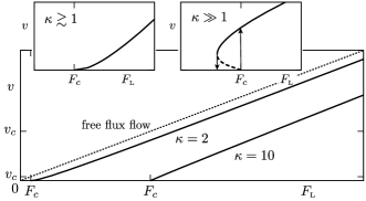
Figure 9: Illustration of the force–velocity curve in the dilute limit for $n_{p}a_{0}\sigma^{2}\kappa=0.05$. In the absence of pinning, the velocity is given by $v=F_{\rm\scriptscriptstyle L}/\eta$ (dotted line). In the presence of pinning, this line is shifted to $F_{c}\propto n_{p}$ (solid line) and closely follows a shifted straight line of equal slope for velocities $v\ll v_{p}$. Corrections to this linear excess-force characteristic appear at velocities beyond $v_{p}$, which does not depend on the small pin density $n_{p}$, or at small velocities $\propto n_{p}^{2}$ (see insets, the arrows refer to the hysteretic switching). Original figure published in Ref. [thomann_12, ].

Besides the corrections at high velocities $v>v_{p}$ due to the velocity dependence of $\langle f_{p}(v)\rangle$, additional changes show up close to $F_{c}$ and at very low velocities due to the square-root dependence $\langle F_{p}(v)\rangle-F_{c}\propto\pm\sqrt{v/v_{p}}$. The force balance equation then can be written in the form

$$\frac{F_{\rm\scriptscriptstyle L}}{F_{c}}-1=\frac{v}{v_{c}}\pm\sqrt{\frac{v}{v_{p}^{\pm}}},$$ (123)

with the small-velocity pinning scales $v_{p}^{\pm}$ deriving from Eq. (112),

$$v_{p}^{-} \sim \frac{\lambda^{2}}{a_{0}^{2}}v_{p},\quad\kappa\gg 1$$ (124)

$$v_{p}^{+} \sim \frac{\lambda^{2}}{a_{0}^{2}}(\kappa-1)^{4}\,v_{p},\quad\kappa\to 1.$$ (125)

For strong pinning $\kappa\gg 1$, the negative (non-linear) correction in the average pinning-force density generates a bistability (and hence hysteretic jumpslarkin_86 ) on the scale $v_{\mathrm{nl}}=v_{c}^{2}/v_{p}^{-}\propto n_{p}^{2}$. The unstable branch increases below $F_{c}$ according to $v\approx v_{p}^{-}(1-F_{\rm\scriptscriptstyle L}/F_{c})^{2}$, turns around reaching a finite value $v=v_{\mathrm{nl}}$ at $F_{\rm\scriptscriptstyle L}=F_{c}$, and approaches the linear excess characteristic $v\approx v_{c}(F_{\rm\scriptscriptstyle L}/F_{c}-1)>v_{\mathrm{nl}}$ for $F_{\rm\scriptscriptstyle L}>F_{c}$. On the other hand, approaching the Labusch point $\kappa\to 1$, the correction changes sign and the velocity increases quadratically,

$$v\sim v_{p}^{+}(F_{\rm\scriptscriptstyle L}/F_{c}-1)^{2}<v_{c}^{2}/v_{p}^{+}=v_{\mathrm{nl}},$$ (126)

reaches the value $v_{\mathrm{nl}}$ at $F_{\rm\scriptscriptstyle L}/F_{c}=1+2v_{c}/v_{p}^{+}$, and crosses over to the linear regime $v\approx v_{c}(F_{\rm\scriptscriptstyle L}/F_{c}-1)>v_{\mathrm{nl}}$ at larger drive $F_{\rm\scriptscriptstyle L}>F_{c}$. While these features are illustrated in the insets of Fig. 9 (showing an expanded view of the characteristic near onset), we have to caution the reader that these results, residing in the regime $v_{\mathrm{nl}}\propto n_{p}^{2}$, may get modified due to collective pinning effects.

VI Model pins

In our discussion above, we have frequently made use of the Lorentzian-shaped pinning potential Eq. (4) in order to gain insights into the strong-pinning features of the dynamical vortex-response. This specific example of a pinning potential is quite appropriate when performing a numerical analysis but is less convenient for analytical studies. The latter can be easily attacked for a bare pinning force $f_{p}(x)$ of polynomial form, at least in the static limit where we have to solve the self-consistency equation (23). It turns out, that for a linear-force profile, the analytic solution can be pushed further to finite velocities, motivating our study of pins with a truncated quadratic (or parabolic) pinning potential, see Fig. 10. However, the quadratic-potential pin formally describes a very strong pin with a Labusch parameter $\kappa\to\infty$, since the force jumps to zero at the pin’s edges at $x=\pm\sigma$. In order to study pinning at intermediate values of $\kappa$ and the approach to the Labusch point $\kappa\to 1$, a more regular potential is required near the force maximum. The results of such an analysis for a cubic pin (or quadratic-force model), although analytically accessible in the static limit, are somewhat cumbersome and we refer the interested reader to Ref. [thomann_thesis, ].

VI.1 Parabolic pin, linear-force model

A simple model for a strong pin is provided by the parabolic potential with the linear pinning-force restricted to a finite interval $[-\sigma,\sigma]$ [see Fig. 10(a)]

$$f_{p}(u)=\left\{\begin{array}[]{l l}-f_{p}\,u/\sigma,&|u|<\sigma,\\ \vspace{3pt}\cr 0,&\mathrm{otherwise}.\end{array}\right.$$ (127)

Given the jumps in the force at the boundaries $\pm\sigma$, the Labusch parameter $\kappa=f_{p}^{\prime}(\pm\sigma)/\bar{C}\to\infty$ and the pin is strong for all values of $f_{p}$. As a consequence, any parabolic potential will produce vortex pinning, e.g., in numerical simulations Olson . On the other hand, the properties of the pin are determined by the dimensionless parameter (see Eq. (29) and the different sign used here)

$$\bar{\kappa}=-{\partial_{x}f_{p}(x)}/{\bar{C}}=f_{p}/\sigma\bar{C},$$ (128)

which is of the same scale as the Labusch parameter $\kappa$ for a similar smooth pin, but should not be confused with the Labusch parameter itself. Piecewise linear models of this type have been considered before in Refs. [matsushita_79, ] using a simplified description of the system’s elastic properties. Furthermore, Larkin and Ovchinnikov larkin_86 used a periodic version of this model in a small-velocity analysis of the strong-pinning physics for large defects.

In the static situation, we have to solve the self-consistency equation (23) for the displacement field $u_{s}(x)$ and we obtain the result

$$u_{s}^{f}(x) = x,\quad|x|>x_{s}^{f}=\sigma,$$ (129)

$$u_{s}^{p}(x) = \frac{x}{1+\bar{\kappa}},\quad|x|<x_{s}^{p}=\sigma(1+\bar{\kappa}),$$ (130)

with the jump points $-x_{s}^{f}$ and $x_{s}^{p}$ for a right moving vortex separated by $\sigma(2+\bar{\kappa})$. The displacement field $u_{s}(x)$ then suddenly changes slope to generate the effective static force $f_{p}[u_{s}(x)]=-\bar{C}x/(1+{\bar{\kappa}}^{-1})\textsection$. Note that the jumps at $-x_{s}^{f}$ (by $\sigma\bar{\kappa}/(1+\bar{\kappa})$) and at $x_{s}^{p}$ (by $\sigma\bar{\kappa}$) do not disappear for any values of $\bar{\kappa}$ and hence the pin is always strong. The critical force Eq. (24) assumes the value

$$F_{c} = n_{p}f_{p}\frac{2t_{\perp}}{a_{0}^{2}}\int_{-x_{s}^{f}}^{x_{s}^{p}}\frac{dx}{\sigma}\,\frac{x}{1+\bar{\kappa}}$$ (131)

$$= \frac{2\bar{\kappa}\sigma^{2}}{a_{0}^{2}}n_{p}f_{p}\,\frac{1+\bar{\kappa}/2}{1+\bar{\kappa}},$$

where we have used $t_{\perp}=x_{s}^{f}=\sigma$ in the last equation. The factor $2\bar{\kappa}\sigma^{2}$ should be interpreted as the trapping area $S_{\mathrm{trap}}$, see also Refs. [ivlev_91, ; blatter_04, ].

Next, we turn to the low-velocity dynamics (see Fig. 10) and determine the coordinate shift $\delta x[u_{s}](x)$ inside the pinning interval $[-x_{s}^{f},x_{s}^{p}]$, see Eq. (100),

$$\delta x[u_{s}](x)=-\frac{2}{\pi}\frac{\sigma\bar{\kappa}}{1+\bar{\kappa}}\frac{1+2x/\sigma}{\sqrt{1+x/\sigma}}\sqrt{\frac{v}{v_{\sigma}}}.$$ (132)

The divergence at $x=-\sigma$ is cut (at $\sim vt_{\mathrm{th}}$) by the fast single-vortex response at short times $t\sim t_{\mathrm{th}}$ where the 3D Green’s function has to be replaced by the 1D one; the remaining spike is relevant in transforming the static solution $u_{s}(x)$ to the dynamic one $u(x)$. As compared with the result Eq. (100) above, the coordinate shift for the linear force model does not exhibit any logarithmic corrections and hence there will be no term $\propto\sqrt{v}\ln v$ in the pinning-force density $\langle\delta F_{p}(v)\rangle$. In fact, using the result Eq. (132) in the calculation of the pinning-force density Eq. (IV.4.1), we obtain

$$\langle\delta F_{p}(v)\rangle \approx -n_{p}f_{p}\frac{2t_{\perp}}{a_{0}^{2}}\biggl{[}\int_{-x_{s}^{f}}^{x_{s}^{p}}\!\!\frac{dx}{\sigma}\,\frac{\delta x[u_{s}](x)}{1+\bar{\kappa}}-\delta x[u_{s}](x_{s}^{p})\biggr{]}$$ (133)

$$= -\frac{4}{3\pi}\frac{\bar{\kappa}\sigma t_{\perp}}{a_{0}^{2}}n_{p}f_{p}\frac{5+5\bar{\kappa}+2\bar{\kappa}^{2}}{(1+\bar{\kappa})^{2}}\sqrt{\frac{v}{v_{p}}},$$

with $v_{p}=v_{\sigma}(2+\bar{\kappa})$ deriving from the effective pin size $\sigma(2+\bar{\kappa})$. As discussed above, the pinning force is reduced $\propto\sqrt{v/v_{p}}$ with respect to the static critical force in the strong pinning situation discussed here. A result similar to Eq. (133) was obtained by Larkin and Ovchinnikov larkin_86 in a periodic linear model for large defects.

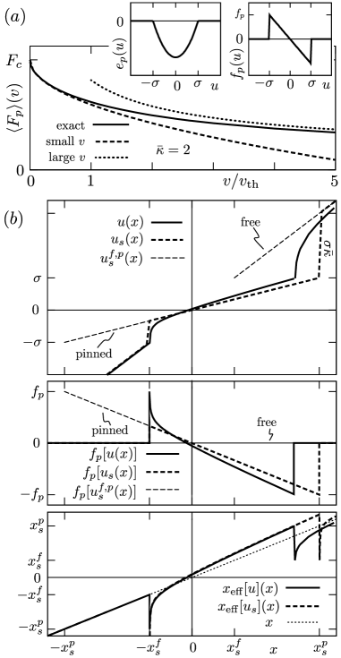
Figure 10: a) Pinning-force density versus velocity for a linear-force pinning model with strength $\bar{\kappa}=2$ (the insets show a sketch of the bare pinning potential $e_{p}(x)$ and bare force $f_{p}(x)$). The exact result (solid) is plotted for comparison with the results from the low- (dashed) and high velocity (dotted) expansions. b) from top to bottom: displacement field $u(x)$, force $f_{p}[u(x)]$, and effective coordinate $x_{\mathrm{eff}}[u](x)$ for a small velocity $v/v_{p}=0.05$. The exact displacement field $u(x)$ and force $f_{p}\bigl{[}u(x)\bigr{]}$ (solid lines) are compared to the static quantities $u_{s}(x)$ and $f_{p}\bigl{[}u_{s}(x)\bigr{]}$ (dashed) for vortex motion from left to right. Also shown are the free [$u_{s}^{f}(x)$ and $f_{p}[u_{s}^{f}(x)]$, light dashed] and pinned branches [$u_{s}^{p}(x)$ and $f_{p}[u_{s}^{p}(x)]$, light dashed], with the multi-valued static solution within the interval $x_{s}^{f}<|x|<x_{s}^{p}$. The exact effective coordinate $x_{\mathrm{eff}}[u](x)$ (solid line) is compared to the approximation $x_{\mathrm{eff}}[u_{s}](x)$ (dashed).

Going to the limit of high velocities $v\gg\bar{\kappa}v_{p}$, we first determine the lowest-order correction to the displacement field, see Eq. (60),

$$u_{p}(x) = -\frac{2\,\bar{\kappa}}{\pi}\frac{\partial}{\partial x}\int_{-\sigma}^{x}dx^{\prime}x^{\prime}\sqrt{\frac{x-x^{\prime}}{vt_{\mathrm{th}}}}$$

$$= -\frac{2\,\bar{\kappa}\sigma}{3\pi}\sqrt{\frac{v_{\sigma}}{v}}\Bigl{(}\frac{2x}{\sigma}-1\Bigr{)}\sqrt{1+\frac{x}{\sigma}}$$

for $-\sigma<x<\sigma$, see Fig. 11. Using the perturbative expression Eq. (IV.2) for the pinning force (note that $f_{p}^{\prime}(x)$ includes a $\delta$-function), we arrive at the result (cf. Eq. (61))

$$\langle F_{p}(v)\rangle \approx \frac{12\sqrt{2}}{5\pi}\,\frac{\sigma t_{\perp}}{a_{0}^{2}}n_{p}f_{p}\sqrt{\frac{\bar{\kappa}^{2}v_{\sigma}}{v}}.$$ (135)

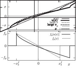
Figure 11: Displacement field $u(x)$ and corresponding force $f_{p}[u(x)]$ at a high velocity $v/v_{p}=2$ and for a pinning parameter $\bar{\kappa}=2$. The exact results (solid lines) are compared with the high-velocity perturbative (dashed) and free (light dotted) results.

The linear-force model also allows for an exact solution of the dynamical situation; within the interval $u\in[-\sigma,\sigma]$ the self-consistency equations (23) and (82) assume the form

$$u(x) = \frac{x-\delta x[u](x)}{1+\bar{\kappa}},$$ (136)

$$\delta x[u](x) = -\frac{f_{p}}{\sigma}\frac{\partial}{\partial x}\int_{-\sigma}^{x}dx^{\prime}G^{\uparrow}(x-x^{\prime})u(x^{\prime}).$$ (137)

This problem can be solved exactly via a Laplace transform and we obtain the solutionLT

$$u(z) = \frac{1}{z^{2}(1+\bar{\kappa}g(z))},$$ (138)

$$g(z) = e^{zvt_{\mathrm{th}}}\mathrm{erfc}(\sqrt{zvt_{\mathrm{th}}}),$$ (139)

with $\mathrm{erfc}(x)$ the complementary error function. Unfortunately, the final solution involves an inverse Laplace transform which cannot be done in closed form,

$$u(x) = \frac{x-\bar{\kappa}\sigma}{1+\bar{\kappa}}+\sigma\bar{\kappa}\int_{0}^{\infty}\frac{ds}{\pi}\Bigl{(}\frac{v/v_{\mathrm{th}}}{s^{2}}+\frac{1}{s}\Bigr{)}$$

$$\quad\times\frac{(1-e^{-s(1+x/\sigma)v_{\sigma}/v})e^{-s}\mathrm{erfi}(\sqrt{s})}{(1+\bar{\kappa}e^{-s})^{2}+\bar{\kappa}^{2}e^{-2s}\mathrm{erfi}^{2}(\sqrt{s})},$$

where $\mathrm{erfi}(x)$ denotes the imaginary error function. The result of the numerical evalution of (VI.1) is shown in Fig. 10, together with the results of the fast- and the slow-velocity analysis.

In the final step, we make use of the mean pinning-force density $\langle F_{p}(v)\rangle$ in the solution of the force-balance equation (1) and find the force–velocity characteristic, see Fig. 12. For small velocities $v\ll v_{p}$, the force balance equation assumes the form

$$\eta v+F_{c}(1-\beta\sqrt{v/v_{p}})=F_{\rm\scriptscriptstyle L},$$ (141)

with

$$\beta = \frac{4}{3\pi}\frac{5+5\bar{\kappa}+2\bar{\kappa}^{2}}{(2+\bar{\kappa})(1+\bar{\kappa})}\stackrel{{\scriptstyle\bar{\kappa}\to\infty}}{{\longrightarrow}}\frac{8}{3\pi}$$ (142)

determined from Eq. (133). The pinning-force density, decreasing with velocity via a square-root law, outperforms the linear behavior of the viscous force density $\eta v$ at small $v$. As a consequence, the force–velocity relation is bistable with (we define the small parameter $\nu=\beta^{2}v_{c}/4v_{p}\sim n_{p}\bar{\kappa}\sigma^{2}a_{0}\ll 1$)

$$\frac{v}{v_{c}}\approx\nu\left(1\pm\sqrt{1+\frac{1}{\nu}\frac{F_{\rm\scriptscriptstyle L}-F_{c}}{F_{c}}}\right)^{2}.$$ (143)

Eq. (143) describes an unstable characteristic $v/v_{c}\approx(1/4\nu)(1-F_{\rm\scriptscriptstyle L}/F_{c})^{2}$ at small $v$ and a jump $\delta v/v_{c}\approx 4\nu$ at $F_{\rm\scriptscriptstyle L}=F_{c}$, see Fig. 12, as also noted by Larkin and Ovchinnikov in their pinning analysis of large defects larkin_86 . The bistability regime extends over a region of size $\propto n_{p}^{2}$ both along the force- and along the velocity axes; specifically, bistability appears within the force interval $1-\nu<F_{\rm\scriptscriptstyle L}/F_{c}<1$ and for velocities $v/v_{c}<4\nu$. The electric field $E_{c}$ corresponding to the jump velocity $4\nu v_{c}$ can be expressed through the critical current density $j_{c}$ and the flux-flow resisitivity $\rho_{\mathrm{ff}}$, $E_{c}=4\nu\rho_{\mathrm{ff}}j_{c}\sim(\kappa n_{p}\sigma^{2}a_{0})\rho_{\mathrm{ff}}j_{c}$, with $\kappa n_{p}\sigma^{2}a_{0}\ll 1$ assuring the dilute pinning limit.

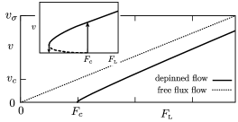
Figure 12: The exact force-density–velocity (current–voltage) relation for parabolic pins with strength $\bar{\kappa}=f_{p}/\sigma\bar{C}=2$. The pinning velocity scale $v_{p}=2v_{\sigma}$ is much larger than the viscous velocity scale $v_{c}=F_{c}/\eta$. Note the bistability for values of the Lorentz force density $F_{\rm\scriptscriptstyle L}$ close to the critical force-density $F_{c}$ (inset), leading to the appearance of jumps larkin_86 . This bistable regime extends over a region of size $\propto n_{p}^{2}$ both in force and in velocity. For large values of $F_{\rm\scriptscriptstyle L}$, free flux flow (dashed) is approached.

Above the critical drive $F_{\rm\scriptscriptstyle L}-F_{c}\ll F_{c}$, we find the linear shape $v/v_{c}\approx F_{\rm\scriptscriptstyle L}/F_{c}-1$. Hence, the force–velocity relation is dominated by the static pinning-force density $F_{c}\propto n_{p}$ and the viscous force density $\eta v$. For large velocities, we use $\langle F_{p}(v)\rangle$ from the expansion Eq. (135) and find the correction around flux flow

$$v\sim\frac{F_{\rm\scriptscriptstyle L}}{\eta}-\frac{4\sqrt{2}}{3\pi}\frac{\bar{\kappa}\sigma t_{\perp}}{a_{0}^{2}}\frac{n_{p}f_{p}}{\eta}\sqrt{\frac{v_{\sigma}}{v_{c}}\frac{F_{c}}{F_{\rm\scriptscriptstyle L}}}.$$ (144)

The linear-force model always resides in the strong pinning limit with $\kappa=\infty$. The most relevant point in the pinning process, the point $x_{s}^{p}=\sigma(\bar{\kappa}+1)$ where the vortex jumps out of the pin, then coincides with the point of maximal (negative) force with $u_{s}(x_{s}^{p})=\sigma$ at the pin boundary. In order to analytically study the dynamical pinning force at smaller values of $\kappa$ including the approach to the Labusch point, one has to choose a smooth shape for the pinning potential. Demanding that the static limit is still analytically solvable, one may choose a cubic potential with the quadratic force profile

$$f_{p}(x)=f_{p}\left\{\begin{array}[]{l l}\displaystyle-(x/\sigma)^{2}-x/\sigma,&-\sigma<x<0,\\ \\ \displaystyle(x/\sigma)^{2}-x/\sigma,&0<x<\sigma,\end{array}\right.$$ (145)

and zero otherwise. This model pin then comes with a tunable Labusch parameter

$$\kappa=\max_{x}\frac{\partial_{x}f_{p}(x)}{\bar{C}}=\frac{\partial_{x}f_{p}(\pm\sigma)}{\bar{C}}=\frac{f_{p}}{\sigma\bar{C}}$$ (146)

and can still be solved analytically in the static limit, that provides the basis for an approximate solution of its dynamical behavior. Since the results are rather cumbersome, we refer the reader to the original solution in Ref. [thomann_thesis, ].

VII Conclusion

We have analyzed the dynamics of the vortex lattice in the presence of dilute strong pins characterized by a Labusch parameter $\kappa>1$ and have determined the strong-pinning force–velocity (or current–voltage) characteristic in the single-pin single-vortex limit. The basic task is the solution of a nonlinear integral equation for the displacement field $u(x=vt)$ describing the vortex tip position when traversing the pin while the vortex ends at $z\sim\pm\infty$ move with constant velocity $v$. The average $\langle f_{p}(v)\rangle$ over the individual pinning forces $f_{p}[u(x)]$ and a proper determination of the velocity dependence of the transverse trapping length $t_{\perp}(v)$ provide the velocity-dependent mean pinning-force density $\langle F_{p}(v)\rangle$. In a last step, we find the mean velocity $v(F_{\rm\scriptscriptstyle L})$ as a function of the driving Lorentz-force density $F_{\rm\scriptscriptstyle L}$—the force–velocity or current–voltage characteristic—by solving the force balance equation $\eta v=F_{\rm\scriptscriptstyle L}-\langle F_{p}(v)\rangle$.

The self-consistent dynamical integral equation for the displacement field $u(x)$ can be solved numerically by simple forward integration due to causality. Such a numerical solution has been carried out for the Lorentzian-shaped pin in order to determine the dynamical effective pinning force $f_{p}[u(x)]$ and the dependence of the pinning force $\langle f_{p}(v)\rangle$ on the velocity $v$. In the static limit, the integral can be separated and the problem simplifies to an algebraic one. The appearance of a multi-valued static solution characterizes a strong pin and allows for a finite static critical force $f_{c}=\langle f_{p}(v=0)\rangle$; the latter is a consequence of the asymmetric occupation of free and pinned branches as the moving vortex jumps into and out of the pin. At finite velocities, the jumps in the static solution $u_{s}(x)$ give way to a unique smooth and asymmetric solution $u(x)$ and the force $f_{p}[u(x)]$ derives from a direct integration without invoking an asymmetric occupation.

The velocity dependence of the dynamical pinning force $\langle f_{p}(v)\rangle$ is governed by the elastic properties of the vortex system as expressed through the Green’s function. Its velocity scale is given by $v_{p}=\kappa v_{\sigma}=\kappa\sigma/t_{\mathrm{th}}$, where $\kappa$ and $\sigma$ encode properties of the pins and $t_{\mathrm{th}}$ is the timescale for the dissipative relaxation of an elastic deformation. At small velocities, a perturbative treatment away from the static solution provides a decrease $\langle\delta f_{p}(v)\rangle\propto-\sqrt{v/v_{p}}$ of the pinning-force density at large values of $\kappa\gg 1$ and an increase $\langle\delta f_{p}(v)\rangle\propto\sqrt{v/v_{p}}$ for small values $\kappa\gtrsim 1$. Indeed, a correction of positive sign $\langle\delta f_{p}(v)\rangle\propto\sqrt{v/v_{p}}\log(v_{p}/v)$ shows up in a small region as $v\to 0$ for any value of $\kappa$, however, this region is exponentially small at large $\kappa$. Increasing the velocity beyond $(a_{0}/\lambda)^{2}v_{p}$, the 3D bulk response gives way to a region of 4D dispersive behavior and $\langle\delta f_{p}(v)\rangle\propto v/v_{p}$ changes linearly with velocity. At high velocities $v>v_{p}$, the rapid motion is dominated by the 1D single-vortex response; furthermore, a self-consistent analysis of the problem shows that the longitudinal trapping or pinning length decreases from $\sim\kappa\sigma$ to $\sim\sigma$, producing a rapid drop in the pinning force $\langle\delta f_{p}(v)\rangle\rangle\propto v_{p}/v$. The $v_{p}/v$ decay of $\langle f_{p}(v)\rangle$ extends over a large velocity regime $v_{p}<v<\kappa v_{p}$ and has not been known before. Finally, perturbation theory away from free flux flow can be performed at high velocities $v\gg\kappa v_{p}$ where pinning is always effectively weak and which provides a generic correction $\langle\delta f_{p}(v)\rangle\propto(\kappa v_{p}/v)^{1/2}$.

The pinning-force density $\langle F_{p}(v)\rangle\approx n_{p}(2t_{\perp}(v)/a_{0})$ $\langle f_{p}(v)\rangle$ follows from simple averaging via direct summation over independent pins, once the dynamical transverse pinning length $t_{\perp}(v)$ has been determined. The latter can be found by studying the trapping process for a vortex approaching the defect with a finite impact parameter and at finite velocity; it turns out that the trapping length decreases from its static value $t_{\perp}\sim\sigma\kappa^{1/(n+2)}$ to $t_{\perp}\sim\sigma$ as the velocity increases to $v_{p}$.

Our study provides access to several types of results, i) exact ones deriving from numerical integration for specific defect potentials $e_{p}(r)$ and ii) perturbative analytic results in the static- and high-velocity limits. Quite remarkable are, iii) the universal results obtained in the large-$\kappa$ limit, with a linear force $f_{p}[u_{s}(x)]\approx-\bar{C}x$ appearing in the static limit and a square-root force $f_{p}[u(x)]\approx-(2/\pi)\bar{C}\sqrt{vt_{\mathrm{th}}x}$ in the intermediate velocity regime $v_{p}<v<\kappa v_{p}$. Finally, iv) dimensional estimates provide us with simple qualitative results for the evolution of $\langle F_{p}(v)\rangle$ with changing velocity $v$ and for all values of $\kappa$. v) Numerical and analytic calculations for a parabolic model-potential give additional insights into the pinning dynamics. Such parabolic pins have often been used in numerical simulations of vortex dynamics in disorder landscapes Olson and always reside in the strong-pinning limit due to their sharp boundary.

The analysis of the velocity-dependent pinning-force density $\langle F_{p}(v)\rangle$ provides us with the velocity scale $v_{p}$ governing the relaxation of the vortex motion across the pinning centers. In the limit of a dilute density $n_{p}$ of pins (where pinning centers act individually) this velocity is much larger than the velocity scale $v_{c}=F_{c}/\eta$ describing the overall motion of the vortex system after depinning. It is this separation of velocities that produces a simple force–velocity or current–voltage characteristic in the strong pinning situation with a dilute density of pins: after depinning at $F_{c}$ (or $j_{c}$), the characteristic evolves first in parallel to free flux-flow (excess-force characteristic $v\sim(F_{\rm\scriptscriptstyle L}-F_{c})/\eta$) and approaches the free flow behavior $v\sim F_{\rm\scriptscriptstyle L}/\eta$ only at very high velocities $v>v_{p}\gg v_{c}$. With our derivation of the excess-force characteristic for the strongly-pinned vortex system in the dilute-pin limit, we have derived the analogue of Coulomb’s law of dry friction for strong vortex pinning—it would be interesting to see if the ideas leading to this result could be applied to other problems of dry friction. Additional nonlinear corrections (corresponding to corrections of Coulomb’s law), a jump at very strong pinning with $\kappa\gg 1$ and a smooth onset for $\kappa\gtrsim 1$ appear in a narrow region of size $\propto n_{p}^{2}$ near depinning; however, a word of caution is in place as results in this regime may get modified by collective pinning effects.

Our theoretical results compare well to a number of experimentally measured current–voltage characteristics strnad_kim_64_65 ; huebener_79 ; berghuis_93 ; zeldov_02 ; pace_04 . The linear excess-current characteristic reported in early experiments was discussed by Campbell and Evettscampbell_72 and by Campbellcampbell_78 , however, no ‘microscopic’ derivation of this basic result has been provided so far. Unfortunately, one has to admit that even today, no systematic studies of experimental current–voltage characteristics are available: Given a specific material, the defect structure is usually non-trivial and may include a variety of pin types. Furthermore, the parameters characterizing the defects are difficult to find. Experiments with superconductors where defects could be designed, tuned, and properly characterized would provide a great help and motivation in further developing the theory of pinning and allow a better comparison between theory and experiment. Numerical studies based on the time-dependent Ginzburg-Landau theory and aiming at optimizing the pinning landscape have been performed very recently Sadovskyy and it will be interesting to compare our results with this type of numerical effort.

Further work is required on the theoretical side: With our analysis, we have provided an important step in the understanding of the static and dynamical strong pinning behavior and its crossover to weak pinning. However, our study is limited to the single-pin single-vortex situation and one has to include effects of other vortices and correlations between pins in order to arrive at a complete picture. Correlations between pins will generate higher-order corrections in $n_{p}$ both in the static and the low-velocity dynamic behavior and their inclusion is a crucial element in the full understanding of the weak to strong pinning crossover.

- (1) H. Kamerlingh Onnes, RN, 14, 818 (1912).
- (2) W. Meissner and R. Ochsenfeld, Naturwissenschaften 21, 787 (1933).
- (3) L.V. Shubnikov, V.I. Khotkevich, Y.D. Shepelev, and Y.N. Riabinin, [Zh. Eksp. Teor. Fiz. 7, 221 (1937)] Ukrainian Journal of Physics 53, 42 (2008).
- (4) A.A. Abrikosov, Sov. Phys. JETP 5, 1174 (1957).
- (5) J. Bardeen and M.J. Stephen, Phys. Rev. 140, A1197 (1965).
- (6) R. Labusch, Cryst. Lattice Defects 1, 1 (1969).
- (7) A.M. Campbell and J.E. Evetts, Adv. Phys. 21, 199 (1972).
- (8) A.I. Larkin and Yu.N. Ovchinnikov, J. Low Temp. Phys. 34, 409 (1979).
- (9) A.I. Larkin, Sov. Phys. JETP 31, 784 (1970).
- (10) G. Blatter et al., Rev. Mod. Phys. 66, 1125 (1994).
- (11) E.H. Brandt, Rep. Prog. Phys. 58, 1465 (1995); T. Nattermann and S. Scheidl, Adv. Phys. 49, 607 (2000).
- (12) A.M. Campbell, Philos. Mag. B 37, 149 (1978).
- (13) T. Matshushita, E. Kusayanagi, and K. Yamafuji, J. Phys. Soc. Jpn. 46, 1101 (1979). T. Matshushita, ibid 46, 1109 (1979); T. Matshushita and K. Yamafuji, ibid 47, 1426 (1979); ibid 50, 38 (1981).
- (14) A.I. Larkin and Yu.N. Ovchinnikov, in Nonequilibrium Superconductivity, edited by D.N. Langenberg and A.I. Larkin (Elsevier, Amsterdam, 1986), p. 493.
- (15) Yu.N. Ovchinnikov and B.I. Ivlev, Phys. Rev. B 43, 8024 (1991).
- (16) A.E. Koshelev and A.B. Kolton, Phys. Rev. B 84, 104528 (2011).
- (17) R. Willa, V.B. Geshkenbein, R. Prozorov, and G. Blatter, Phys. Rev. Lett. 115, 207001 (2015); R. Willa, V.B. Geshkenbein, and G. Blatter, Phys. Rev. B 92, 134501 (2015).
- (18) R. Willa, V.B. Geshkenbein, and G. Blatter, Phys. Rev. B 93, 064515 (2016).
- (19) G. Blatter, V.B. Geshkenbein, and J.A.G. Koopmann, Phys. Rev. Lett. 92, 067009 (2004).
- (20) A. Schmid and W. Hauger, J. Low Temp. Phys. 11, 667 (1973).
- (21) A.I. Larkin and Yu.N. Ovchinnikov, Sov. Phys. JETP 38, 854 (1974).
- (22) O. Narayan and D.S. Fisher, Phys. Rev. B 46, 11520 (1992); P. Chauve, T. Giamarchi, and P. Le Doussal, Phys. Rev. B 62, 6241 (2000).
- (23) A.R. Strnad, C.F. Hempstead, and Y.B. Kim, Phys. Rev. Lett. 13, 794 (1964); Y.B. Kim, C.F. Hempstead, and A.R. Strnad, Phys. Rev. 139, 1163 (1965).
- (24) R.P. Huebener, in Magnetic Flux Structures in Superconductors (Springer-Verlag, Berlin, 1979).
- (25) P. Berghuis and P.H. Kes, Phys. Rev. B 47, 262 (1993).
- (26) Z.L. Xiao, E.Y. Andrei, Y. Paltiel, E. Zeldov, P. Shuk, and M. Greenblatt, Phys. Rev. B 65, 094511 (2002).
- (27) S. Pace, G. Filatrella, G. Grimaldi, and A. Nigro, Phys. Lett. A 329, 379 (2004).
- (28) C. Reichhardt, C.J. Olson, J. Groth, S. Field, and F. Nori, Phys. Rev. B 52, 10441 (1995); C.J. Olson Reichhardt, Y.L. Wang, Z.L. Xiao, W.K. Kwok, D. Raya, C. Reichhardt, B. Jankó, Physica C 533 (2017).
- (29) A.U. Thomann, V.B. Geshkenbein, and G. Blatter, Phys. Rev. Lett. 108, 217001 (2012).
- (30) E.V. Thuneberg, J. Kurkijärvi, and D. Rainer, Phys. Rev. B 29, 3913 (1984).
- (31) A. Schmid, Phys. Kondens. Materie 5, 302 (1966).
- (32) J.R. Clem, J. Low Temp. Phys. 18, 427 (1975).
- (33) Note that we distinguish defect and vortex positions only by roman and greek indices, implying that these are not to be replaced by equal numbers.
- (34) Note that a precise determination of requires a numerical analysis, see the discussion in Ref. [willa_16, ].
- (35) C.M. Bender and S.A. Orszag, Advanced Mathematical methods for scientists and engineers (McGraw-Hill, New York, 1978), page 150.
- (36) Note that the limit at fixed would take us out of the single-pin regime: while , stays finite. The condition to remain in the strong pinning regime then reads , which requires that .
- (37) A. Thomann, in Dynamical Instabilities in Superconducting Systems, ETH thesis #19808 (2011).
- (38) We define the Laplace transform as and its inverse via .
- (39) I.A. Sadovskyy, Y. Jia, M. Leroux, J. Kwon, H. Hu, L. Fang, C. Chaparro, S. Zhu, U. Welp, J.-M. Zuo, Y. Zhang, R. Nakasaki, V. Selvamanickam, G.W. Crabtree, A.E. Koshelev, A. Glatz, W.-K. Kwok, Adv. Mater. 28, 4593 (2016).