Deploy-As-You-Go Wireless Relay Placement: An Optimal Sequential Decision Approach using the Multi-Relay Channel Model

Abstract

We use information theoretic achievable rate formulas for the multi-relay channel to study the problem of as-you-go deployment of relay nodes. The achievable rate formulas are for full-duplex radios at the relays and for decode-and-forward relaying. Deployment is done along the straight line joining a source node and a sink node at an unknown distance from the source. The problem is for a deployment agent to walk from the source to the sink, deploying relays as he walks, given the knowledge of the wireless path-loss model, and given that the distance to the sink node is exponentially distributed with known mean. As a precursor to the formulation of the deploy-as-you-go problem, we apply the multi-relay channel achievable rate formula to obtain the optimal power allocation to relays placed along a line, at fixed locations. This permits us to obtain the optimal placement of a given number of nodes when the distance between the source and sink is given. Numerical work for the fixed source-sink distance case suggests that, at low attenuation, the relays are mostly clustered close to the source in order to be able to cooperate among themselves, whereas at high attenuation they are uniformly placed and work as repeaters. We also prove that the effect of path-loss can be entirely mitigated if a large enough number of relays are placed uniformly between the source and the sink. The structure of the optimal power allocation for a given placement of the nodes, then motivates us to formulate the problem of as-you-go placement of relays along a line of exponentially distributed length, and with the exponential path-loss model, so as to minimize a cost function that is additive over hops. The hop cost trades off a capacity limiting term, motivated from the optimal power allocation solution, against the cost of adding a relay node. We formulate the problem as a total cost Markov decision process, establish results for the value function, and provide insights into the placement policy and the performance of the deployed network via numerical exploration.

1 Introduction

Wireless interconnection of devices such as smart phones, or wireless sensors, to the wireline communication infrastructure is an important requirement. These are battery operated, resource constrained devices. Hence, due to the physical placement of these devices, or due to channel conditions, a direct one-hop link to the infrastructure “base-station” might not be feasible. In such situations, other nodes could serve as relays in order to realize a multi-hop path between the source device and the infrastructure. In the wireless sensor network context, the relays could be other wireless sensors or battery operated radio routers deployed specifically as relays. The relays are also resource constrained and a cost might be involved in placing them. Hence, there arises the problem of optimal relay placement. Such a problem involves the joint optimization of node placement and operation of the resulting network, where by “operation” we mean activities such as transmission scheduling, power allocation, and channel coding.

Figure 1: A source and a sink connected by a multi-hop path comprising $N$ relay nodes along a line.

Our work in this paper is motivated by recent interest in problems of impromptu (as-you-go) deployment of wireless relay networks in various situations; for example, “first responders” in emergency situations, or quick deployment (and redeployment) of sensor networks in large terrains, such as forests (see [3], [4], [5], [6], [7]). In this paper, we are concerned with the situation in which a deployment agent walks from the source node to the sink node, along the line joining these two nodes, and places wireless relays (in an “as-you-go” manner) so as to create a source-to-sink multi-relay channel network with high data rate; see Figure 1. We first consider the scenario where the length $L$ of the line in Figure 1 is known; the results of this case are used to formulate the as-you-go deployment in the case where $L$ is a priori unknown, but has exponential distribution with known mean $\overline{L}$.

In order to capture the fundamental trade-offs involved in such problems, we consider an information theoretic model. For a placement of the relay nodes and allocation of transmission powers to these relays, we model the “quality” of communication between the source and the sink by the information theoretic achievable rate of the multi-relay channel (see [8], [9] and [10] for the single and multi-relay channel models). The relays are equipped with full-duplex radios, and carry out decode-and-forward relaying. We consider scalar, memoryless, time-invariant, additive white Gaussian noise (AWGN) channels. We assume synchronous operation across all transmitters and receivers, and consider the exponential path-loss model for radio wave propagation.

1.1 Related Work

A formulation of the relay placement problem requires a model of the wireless network at the physical (PHY) and medium access control (MAC) layers. Most researchers have adopted the link scheduling and interference model, i.e., a scheduling algorithm determines radio resource allocation (channel and power) and interference is treated as noise (see [15]); treating interference as noise leads to the model that simultaneous transmissions “collide” at receiving nodes, and transmission scheduling aims to avoid collisions.

However, node placement for throughput maximization with this model is intractable because the optimal throughput is obtained by first solving for the optimum schedule assuming fixed node locations, followed by an optimization over those locations. Hence, with such a model, there appears to be little work on the problem of jointly optimizing the relay node placement and the transmission schedule. Reference [16] is one such work where the authors considered placing a set of nodes in an existing network such that a certain network utility is optimized subject to a set of linear constraints on link rates, under the link scheduling and interference model. They posed the problem as one of geometric programming assuming exponential path-loss, and proposed a distributed solution. The authors of [17] consider relay placement for utility maximization, assuming there are several source nodes, sink nodes and a few candidate locations for placing relays; they ignore interference because of highly directional antennas used in $60$ GHz mmWave networks, which may not always be valid. Relay placement for capacity enhancement has been studied in [18], but there interference is mitigated by scheduling transmissions over multiple channels.

On the other hand, an information theoretic model for a wireless network often provides a closed-form expression for the channel capacity, or at least an achievable rate region. These results are asymptotic, and make idealized assumptions such as full-duplex radios, perfect interference cancellation, etc., but provide algebraic expressions that can be used to formulate tractable optimization problems which can provide useful insights. In the context of optimal relay placement, some researchers have already exploited this approach. Thakur et al., in [19], report on the problem of placing a single relay node to maximize the capacity of a broadcast relay channel in a wideband regime. Lin et al., in [20], numerically solve the problem of a single relay node placement, under power-law path loss and individual power constraints at the source and the relay; however, our work is primarily focused on multi-relay placement, under the exponential path-loss model and a sum power constraint among the nodes. The linear deterministic channel model ([21]) is used by Appuswamy et al. in [22] to study the problem of placing two or more relay nodes along a line so as to maximize the end-to-end data rate. Our present paper is in a similar spirit; however, we use the achievable rate formulas for the $N$-relay channel (with decode and forward relays) to study the problem of placing relays on a line having length $L$, under a sum power constraint over the nodes.

The most important difference of our paper with the literature reported above is that we address the problem of sequential placement of relay nodes along a line of an unknown random length. This paper extends our previous work in [1], which presents the analysis for the case of given $L$ and $N$; the study under given $L$ and $N$ is a precursor to the formulation of as-you-go deployment problem, since it motivates an additive cost structure that is essential for the formulation of the sequential deployment problem as a Markov decision process (MDP).

The deploy-as-you-go problem has been addressed by previous researchers. For example, Howard et al., in [4], provide heuristic algorithms for incremental deployment of sensors in order to cover a deployment area. Souryal et al., in [3], propose heuristic deployment algorithms for the problem of impromptu wireless network deployment, with an experimental study of indoor RF link quality variation. The authors of [5] propose a collaborative deployment method for multiple deployment agents, so that the contiguous coverage area of relays is maximized subject to a total number of relays constraint. However, until the work in [23] and [6], there appears to have been no effort to rigorously formulate as-you-go deployment problem in order to derive optimal deployment algorithms. The authors of [23] and [6] used MDP based formulations to address the problem of placing relay nodes sequentially along a line and along a random lattice path, respectively. The formulations in [23] and [6] are based on the so-called “lone packet traffic model" under which, at any time instant, there can be no more than one packet traversing the network, thereby eliminating contention between wireless links. This work was later extended in [7] to the scenario where the traffic is still lone packet, but a measurement-based approach is employed to account for the spatial variation of link qualities due to shadowing.

In this paper, we consider as-you-go deployment along a line, but move away from the lone-packet traffic assumption by employing information theoretic achievable rate formulas (for full-duplex radios and decode-and-forward relaying). We assume exponential path-loss model (see [24] and Section 6.1). To the best of our knowledge, there is no prior work that considers as-you-go deployment under this physical layer model.

1.2 Our Contribution

• Optimal Offline Deployment: Given the location of $N$ full-duplex relays to connect a source and a sink separated by a given distance $L$, and under the exponential path-loss model and a sum power constraint among the nodes, the optimal power split among the nodes and the achievable rate are expressed (Theorem 1) in terms of the channel gains. We find expression for optimal relay location in the single relay placement problem (Theorem 2). For the $N$ relay placement problem, numerical study shows that, the relay nodes are clustered near the source at low attenuation and are placed uniformly at high attenuation. Theorem 5 shows that, by placing large number of relays uniformly, we can achieve a rate arbitrarily close to the AWGN capacity. Only this part of our current paper was published in the conference version [1].

• Optimal As-You-Go Deployment: In Section 4, we consider the problem of placing relay nodes in a deploy-as-you-go manner, so as to connect a source and a sink separated by an unknown distance, modeled as an exponentially distributed random variable $L$. Specifically, the problem is to start from a source, and walk along a line, placing relay nodes as we go, until the line ends, at which point the sink is placed. With a sum power constraint, the aim is to maximize a capacity limiting term derived from the deployment problem for known $L$, while constraining the expected number of relays. We “relax” the expected number of relays constraint via a Lagrange multiplier, and formulate the problem as a total cost MDP with uncountable state space and non-compact action sets. We prove the existence of an optimal policy and convergence of value iteration (Theorem 7); these results for uncountable state space and non-compact action space are not evident from standard literature. We study properties of the value function analytically. This is the first time that the as-you-go deployment problem is formulated to maximize the end-to-end data rate under the full-duplex multi-relay channel model.

• Numerical Results on As-You-Go Deployment: In Section 5, we study the policy structure numerically. We also demonstrate numerically that the proposed as-you-go algorithm achieves an end-to-end data rate sufficiently close to the maximum possible achievable data rate for offline placement. This is particularly important since there is no other benchmark in the literature, with which we can make a fair comparison of our policy.

• The material in Section 4 and Section 5 were absent in the conference version [1].

1.3 Organization of the Paper

In Section 2, we describe our system model and notation. In Section 3, we address the problem of relay placement on a line of known length. Section 4 deals with the problem of as-you-go deployment along a line of unknown random length. Numerical work on as-you-go deployment has been presented in Section 5. Some discussions are provided in Section 6. Conclusions are drawn in Section 7.

2 System Model and Notation

2.1 The Multi-Relay Channel

The multi-relay channel was studied in [10] and [9] and is an extension of the single relay model presented in [8]. We consider a network deployed on a line with a source node and a sink node at the end of the line, and $N$ full-duplex relay nodes as shown in Figure 1. The relay nodes are numbered as $1,2,\cdots,N$. The source and sink are indexed by $0$ and $N+1$, respectively. The distance of the $k$-th node from the source is denoted by $y_{k}:=r_{1}+r_{2}+\cdots+r_{k}$. Thus, $y_{N+1}=L$. As in [10] and [9], we consider the scalar, time-invariant, memoryless, AWGN setting.

We use the model that a symbol transmitted by node $i$ is received at node $j$ after multiplication by the (positive, real valued) channel gain $h_{i,j}$ (an assumption often made in the literature, see e.g., [10] and [25]). The power gain from Node $i$ to Node $j$ is denoted by $g_{i,j}=h_{i,j}^{2}$. We define $g_{i,i}=1$ and $h_{i,i}=1$. The Gaussian additive noise at any receiver is independent and identically distributed from symbol to symbol and has variance $\sigma^{2}$.

2.2 An Inner Bound to the Capacity

For the multi-relay channel, we denote the symbol transmitted by the $i$-th node at time $t$ ($t$ is discrete) by $X_{i}(t)$ for $i=0,1,\cdots,N$. $Z_{k}(t)\sim\mathcal{N}(0,\sigma^{2})$ is the additive white Gaussian noise at node $k$ and time $t$, and is assumed to be independent and identically distributed across $k$ and $t$. Thus, at symbol time $t$, node $k,1\leq k\leq N+1$ receives:

$$Y_{k}(t)=\sum_{j\in\{0,1,\cdots,N\},j\neq k}h_{j,k}X_{j}(t)+Z_{k}(t)$$ (1)

An inner bound to the capacity of this network, under any path-loss model, is given by (see [10]):

$$R=\min_{1\leq k\leq N+1}C\bigg{(}\frac{1}{\sigma^{2}\texttimes}\sum_{j=1}^{k}(\sum_{i=0}^{j-1}h_{i,k}\sqrt{P_{i,j}})^{2}\bigg{)}$$ (2)

where $C(x):=\frac{1}{2}\log_{2}(1+x)$, and node $i$ transmits to node $j$ at power $P_{i,j}$ (expressed in mW).

In Appendix A, we provide a descriptive overview of the coding and decoding scheme proposed in [10]. A sequence of messages are sent from the source to the sink; each message is encoded in a block of symbols and transmitted by using the relay nodes. The scheme involves coherent transmission by the source and relay nodes (this requires symbol-level synchronization among the nodes), and successive interference cancellation at the relay nodes and the sink. A node receives information about a message in two ways (i) by the message being directed to it cooperatively by all the previous nodes, and (ii) by overhearing previous transmissions of the message to the previous nodes. Thus node $k$ receives codes corresponding to a message $k$ times before it attempts to decode the message (a discussion on the practical feasibility of full-duplex decode-and-forward relaying scheme is provided in Section 6.3). Note that, $C\bigg{(}\frac{1}{\sigma^{2}\texttimes}\sum_{j=1}^{k}(\sum_{i=0}^{j-1}h_{i,k}\sqrt{P_{i,j}})^{2}\bigg{)}$ in (2), for any $k$, denotes a possible rate that can be achieved by node $k$ from the transmissions from nodes $0,1,\cdots,k-1$. The smallest of these terms becomes the bottleneck, see (2).

For the single relay channel, $N=1$. Thus, by (2), an achievable rate is given by (see also [8]):

$$R=\min \bigg{\{} C\left(\frac{g_{0,1}P_{0,1}}{\sigma^{2}\texttimes}\right),$$ (3)

$$C\left(\frac{g_{0,2}P_{0,1}+(h_{0,2}\sqrt{P_{0,2}}+h_{1,2}\sqrt{P_{1,2}})^{2}}{\sigma^{2}\texttimes}\right)\bigg{\}}$$

Here, the first term in the $\min\{\cdot,\cdot\}$ of (3) is the achievable rate at node $1$ (i.e., the relay node) due to the transmission from the source. The second term in the $\min\{\cdot,\cdot\}$ corresponds to the possible achievable rate at the sink node due to direct coherent transmission from the source and the relay and due to the overheard transmission from the source to the relay. The higher the channel attenuation, the less will be the contribution of farther nodes, “overheard” transmissions become less relevant, and coherent transmission reduces to a simple transmission from the previous relay. The system is then closer to simple store-and-forward relaying.

The authors of [10] have shown that any rate strictly less than $R$ is achievable through the coding and decoding scheme. This achievable rate formula can also be obtained from the capacity formula of a physically degraded multi-relay channel (see [9]), since the capacity of the degraded relay channel is a lower bound to the actual channel capacity. In this paper, we will seek to optimize $R$ in (2) over power allocations to the nodes and the node locations, keeping in mind that $R$ is a lower bound to the actual capacity. We denote the value of $R$ optimized over power allocation and relay locations by $R^{*}$.

2.3 Path-Loss Model

We model the power gain via the exponential path-loss model: the power gain at a distance $r$ is $e^{-\rho r}$ where $\rho>0$. This is a simple model used for tractability (see [16], [22]) and [26, Section $2.3$] for prior work assuming exponential path-loss). However, for propagation scenarios involving randomly placed scatterers (as would be the case in a dense urban environment, or a forest, for example) analytical and experimental support has been provided for the exponential path-loss model (a discussion has been provided in Section 6.1). We also discuss in Section 6.4 how the insights obtained from the results for exponential path-loss can be used for power-law path-loss (power gain at a distance $r$ is $r^{-\eta}$, $\eta>0$). Deployment with other path-loss models is left in this paper as a possible future work.

Under exponential path-loss, the channel gains and power gains in the line network become multiplicative, e.g., $h_{i,i+2}=h_{i,i+1}h_{i+1,i+2}$ and $g_{i,i+2}=g_{i,i+1}g_{i+1,i+2}$ for $i\in\{0,1,\cdots,N-1\}$.

We discuss in Section 6.2 how shadowing and fading can be taken care of in our model, by providing a fade- margin in the power at each transmitter.

2.4 Motivation for the Sum Power Constraint

In this paper we consider the sum power constraint $\sum_{i=0}^{N}P_{i}=P_{T}$ (in mW) over the source and the relays. This constraint has the following motivation. Let the fixed power expended in a relay (for reception and driving the electronic circuits) be denoted by $P_{\mathrm{rcv}}$ (expressed in mW), and the initial battery energy in each node be denoted by $E$ (in mJ unit). The information theoretic approach utilized in this paper requires that the nodes in the network are always on. Hence, the lifetime of node $i,1\leq i\leq N$, is $\tau_{i}=\frac{E}{P_{i}+P_{rcv}\texttimes}$, the lifetime of the source is $\tau_{0}=\frac{E}{P_{0}}$, and that of the sink is $\tau_{N+1}=\frac{E}{P_{rcv}}$. The rate of battery replacement at node $i$ is $\frac{1}{\tau_{i}}$. Hence, the rate at which we have to replace the batteries in the network is $\sum_{i=0}^{N+1}\frac{1}{\tau_{i}\texttimes}=\frac{1}{E\texttimes}(\sum_{i=0}^{N}P_{i}+(N+1)P_{rcv})$. The depletion rate $\frac{P_{rcv}}{E}$ is inevitable at any node, and it does not affect the achievable data rate. Hence, in order to reduce the battery replacement rate, we must reduce the sum transmit power in the entire network.

3 Placement on a Line of Known Length

As a precursor to addressing the deploy-as-you-go problem over a line of unknown length, in this section we solve the problem of power constrained deployment of a given number of relays on a line of known length. We will often refer to this problem as offline deployment problem. The results of this section provide (i) first insights into the relay placements we obtain using the multi-relay channel model, (ii) a starting point for the formulation of as-you-go deployment problem, and (iii) a benchmark with which we can compare the performance of our as-you-go deployment algorithm.

3.1 Optimal Power Allocation

In this section, we consider the optimal placement of relay nodes on a line of given length, $L$, so as to to maximize $R$ (see (2)), subject to a total power constraint on the source and relay nodes given by $\sum_{i=0}^{N}P_{i}=P_{T}$. We will first maximize $R$ in (2) over $P_{i,j},0\leq i<j\leq(N+1)$ for any given placement of nodes (i.e., given $y_{1},y_{2},\cdots,y_{N}$). This will provide an expression of achievable rate in terms of channel gains, which has to be maximized over $y_{1},y_{2},\cdots,y_{N}$. Let $\gamma_{k}:=\sum_{i=0}^{k-1}P_{i,k}$ for $k\in\{1,2,\cdots,N+1\}$ (expressed in mW). Hence, the sum power constraint becomes $\sum_{k=1}^{N+1}\gamma_{k}=P_{T}$.

Theorem 1

1. Under the exponential path-loss model, for fixed location of relay nodes, the optimal power allocation that maximizes the achievable rate for the sum power constraint is given by:

   $$P_{i,j}=\begin{cases}\frac{g_{i,j}}{\sum_{l=0}^{j-1}g_{l,j}\texttimes}\gamma_{j}\,\,&\forall 0\leq i<j\leq(N+1)\\ 0,\,\,&\text{if}\,\,j\leq i\end{cases}$$ (4)

   where

   $$\gamma_{1} = \frac{P_{T}\texttimes}{1+g_{0,1}\sum_{k=2}^{N+1}\frac{(g_{0,k-1}-g_{0,k})}{g_{0,k}g_{0,k-1}\sum_{l=0}^{k-1}\frac{1}{g_{0,l}\texttimes}\texttimes}\texttimes}$$ (5)

   $$\gamma_{j} = \frac{g_{0,1}\frac{(g_{0,j-1}-g_{0,j})}{g_{0,j}g_{0,j-1}\sum_{l=0}^{j-1}\frac{1}{g_{0,l}\texttimes}\texttimes}\texttimes}{1+g_{0,1}\sum_{k=2}^{N+1}\frac{(g_{0,k-1}-g_{0,k})}{g_{0,k}g_{0,k-1}\sum_{l=0}^{k-1}\frac{1}{g_{0,l}\texttimes}\texttimes}\texttimes}P_{T}\,\,\,\,\forall\,j\geq 2$$

2. The achievable rate optimized over the power allocation for a given placement of nodes is given by:

   $$R^{opt}_{P_{T}}(y_{1},y_{2},\cdots,y_{N})=C\bigg{(}\frac{\frac{P_{T}}{\sigma^{2}\texttimes}}{\frac{1}{g_{0,1}\texttimes}+\sum_{k=2}^{N+1}\frac{(g_{0,k-1}-g_{0,k})}{g_{0,k}g_{0,k-1}\sum_{l=0}^{k-1}\frac{1}{g_{0,l}\texttimes}\texttimes}\texttimes}\bigg{)}$$ (6)

Proof:

The basic idea is to choose the power levels (i.e., $P_{i,j},\,0\leq i<j\leq N+1$) in (2) so that all the terms in the $\min\{\cdot\}$ in (2) become equal. We provide explicit expressions for $P_{i,j},\,0\leq i<j\leq N+1$ and the achievable rate (optimized over power allocation) in terms of the power gains. See Appendix B for the detailed proof. A result on the equality of certain terms under optimal power allocation has also been proved in [9] for the coding scheme used in [9]. But it was proved in the context of a degraded Gaussian multi-relay channel, and the proof depends on an inductive argument, whereas our proof utilizes LP (linear programming) duality. ∎

Recalling the exponential path-loss parameter $\rho$, and the source-sink distance $L$, let us define $\lambda:=\rho L$, which can be treated as a measure of attenuation in the line.

Let us now comment on the results of Theorem 1:

• In order to maximize $R^{opt}_{P_{T}}(y_{1},y_{2},\cdots,y_{N})$, we need to place the relay nodes such that $\frac{1}{g_{0,1}}+\sum_{k=2}^{N+1}\frac{(g_{0,k-1}-g_{0,k})}{g_{0,k}g_{0,k-1}\sum_{l=0}^{k-1}\frac{1}{g_{0,l}\texttimes}\texttimes}$ is minimized. This quantity is viewed as the net attenuation the power $P_{T}$ faces.

• When no relay is placed, the attenuation is $e^{\lambda}$. The ratio of attenuation with no relay and attenuation with relays is called the “relaying gain” $G(N,\lambda)$.

  $$G(N,\lambda):=\frac{e^{\lambda}}{\frac{1}{g_{0,1}\texttimes}+\sum_{k=2}^{N+1}\frac{(g_{0,k-1}-g_{0,k})}{g_{0,k}g_{0,k-1}\sum_{l=0}^{k-1}\frac{1}{g_{0,l}\texttimes}\texttimes}\texttimes}$$ (7)

  Rate is increasing with the number of relays, and is bounded above by $C(\frac{P_{T}}{\sigma^{2}})$. Hence, $G(N,\lambda)\in[1,e^{\lambda}]$. Also, note that $G(N,\lambda)$ does not depend on $P_{T}$.

• By Theorem 1, we have $P_{k,j}\geq P_{i,j}$ for $i<k<j$.

• Note that we have derived Theorem 1 using the fact that $g_{0,k}$ is nonincreasing in $k$. If there exists some $k\geq 1$ such that $g_{0,k}=g_{0,k+1}$, i.e, if $k$-th and $(k+1)$-st nodes are placed at the same position, then $\gamma_{k+1}=0$, i.e., the nodes $i<k$ do not direct any power specifically to relay $k+1$. However, relay $k+1$ can decode the symbols received at relay $k$, and those transmitted by relay $k$. Then relay $(k+1)$ can transmit coherently with the nodes $l\leq k$ to improve effective received power in the nodes $j>k+1$.

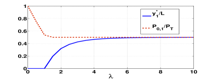
Figure 2: Single relay placement, total power constraint, exponential path-loss: $\frac{y_{1}^{*}}{L\texttimes}$ and optimum $\frac{P_{0,1}}{P_{T}\texttimes}$ versus $\lambda$.

(a) $N=2$

(b) $N=3$

(c) $N=5$

Figure 3: $N$ relays, exponential path-loss model: depiction of the optimal relay positions for $N=2,3,5$ for various values of $\lambda$. On any line, the leftmost dot is the source node, the rightmost dot is the sink, and the intermediate dots denote the relays.

3.2 Optimal Placement of a Single Relay Node

In the following theorem, we derive the optimal power allocation, node location and data rate when a single relay is placed.

Theorem 2

For the single relay node placement problem with sum power constraint and exponential path-loss model, the normalized optimum relay location $\frac{y_{1}^{*}}{L\texttimes}$, power allocation and optimized achievable rate are given as follows:

1. For $\lambda\leq\log 3$, $\frac{y_{1}^{*}}{L\texttimes}=0$, $P_{0,1}=\frac{2P_{T}}{e^{\lambda}+1\texttimes}$, $P_{0,2}=P_{1,2}=\frac{e^{\lambda}-1}{e^{\lambda}+1\texttimes}\frac{P_{T}}{2\texttimes}$ and $R^{*}=C\left(\frac{2P_{T}}{(e^{\lambda}+1)\sigma^{2}\texttimes}\right)$.

2. For $\lambda\geq\log 3$, $\frac{y_{1}^{*}}{L\texttimes}=\frac{1}{\lambda\texttimes}\log\left(\sqrt{e^{\lambda}+1}-1\right)$, $P_{0,1}=\frac{P_{T}}{2\texttimes}$, $P_{0,2}=\frac{1}{\sqrt{e^{\lambda}+1}\texttimes}\frac{P_{T}}{2\texttimes}$, $P_{1,2}=\frac{\sqrt{e^{\lambda}+1}-1}{\sqrt{e^{\lambda}+1}\texttimes}\frac{P_{T}}{2\texttimes}$ and $R^{*}=C\left(\frac{1}{\sqrt{e^{\lambda}+1}-1\texttimes}\frac{P_{T}}{2\sigma^{2}\texttimes}\right)$

Proof:

See Appendix C. ∎

Discussion: It is easy to check that $R^{*}$ obtained in Theorem 2 is strictly greater than the AWGN capacity $C\left(\frac{P_{T}}{\sigma^{2}\texttimes}e^{-\lambda}\right)$ for all $\lambda>0$. This happens because the source and relay transmit coherently to the sink. $R^{*}$ becomes equal to the AWGN capacity only at $\lambda=0$. At $\lambda=0$, we do not use the relay since the sink can decode any message that the relay is able to decode.

The variation of $\frac{y_{1}^{*}}{L\texttimes}$ and $\frac{P_{0,1}}{P_{T}}$ with $\lambda$ has been shown in Figure 2. We observe that (from Figure 2 and Theorem 2) $\lim_{\lambda\rightarrow\infty}\frac{y_{1}^{*}}{L}=\frac{1}{2\texttimes}$, $\lim_{\lambda\rightarrow\infty}P_{0,2}=0$ and $\lim_{\lambda\rightarrow 0}P_{0,1}=P_{T}$. For large values of $\lambda$, source and relay cooperation provides negligible benefit since source to sink attenuation is very high. So it is optimal to place the relay at a distance $\frac{L}{2\texttimes}$. The relay works as a repeater which forwards data received from the source to the sink. For small $\lambda$, the gain obtained from coherent transmission is dominant, and, in order to receive sufficient information (required for coherent transmission) from the source, the relay is placed near the source.

3.3 Optimal Placement for a Multi-Relay Channel

As we discussed earlier, we need to place $N$ relay nodes such that $\frac{1}{g_{0,1}\texttimes}+\sum_{k=2}^{N+1}\frac{(g_{0,k-1}-g_{0,k})}{g_{0,k}g_{0,k-1}\sum_{l=0}^{k-1}\frac{1}{g_{0,l}\texttimes}\texttimes}$ is minimized. Here $g_{0,k}=e^{-\rho y_{k}}$. We have the constraint $0\leq y_{1}\leq y_{2}\leq\cdots\leq y_{N}\leq y_{N+1}=L$. Now, writing $z_{k}=e^{\rho y_{k}}$, and defining $z_{0}:=1$, we arrive at the following problem:

$$\min\bigg{\{}z_{1}+\sum_{k=2}^{N+1}\frac{z_{k}-z_{k-1}}{\sum_{l=0}^{k-1}z_{l}}\bigg{\}}$$ (8)

$$s.t \,\,1\leq z_{1}\leq\cdots\leq z_{N}\leq z_{N+1}=e^{\lambda}$$

The objective function is convex in each of the variables $z_{1},z_{2},\cdots,z_{N}$. The objective function is sum of linear fractionals, and the constraints are linear.

Remark: From optimization problem (8) we observe that optimum $z_{1},z_{2},\cdots,z_{N}$ depend only on $\lambda:=\rho L$. Since $z_{k}=e^{\lambda\frac{y_{k}}{L}}$, the normalized optimal distance of relays from the source depend only on $\lambda$ and $N$.

Theorem 3

For fixed $\rho$, $L$ and $\sigma^{2}$, the optimized achievable rate $R^{*}$ for a sum power constraint strictly increases with the number of relay nodes.

Proof:

See Appendix D. ∎

Theorem 4

For any fixed number of relays $N\geq 1$, $G(N,\lambda)$ is increasing in $\lambda$.

Proof:

See Appendix E. ∎

A numerical study of multi-relay placement: We discretize the interval $[0,L]$ and run a search program to find normalized optimal relay locations for different values of $\lambda$ and $N$. The results are summarized in Figure 3.

We observe that at low attenuation (small $\lambda$), relay nodes are clustered near the source node and are often at the source node, whereas at high attenuation (large $\lambda$) they are almost uniformly placed along the line. For large $\lambda$, the effect of long distance between any two adjacent nodes dominates the gain obtained by coherent relaying. Hence, it is beneficial to minimize the maximum distance between any two adjacent nodes and thus multihopping is a better strategy in this case. For small $\lambda$, the gain obtained by coherent transmission is dominant. In order to allow this, relays should be able to receive sufficient information from their previous nodes. Thus, they tend to be clustered near the source.

In Figure 4 we plot the relaying gain $G(N,\lambda)$ in dB vs. the number of relays $N$, for various values of $\lambda$. As proved in Theorem 3, we see that $G(N,\lambda)$ increases with $N$ for fixed $\lambda$. On the other hand, $G(N,\lambda)$ increases with $\lambda$ for fixed $N$, as proved in Theorem 4.

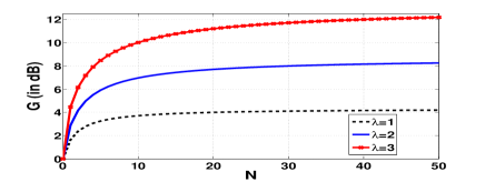
Figure 4: $G(N,\lambda)$ vs $N$ for total power constraint.

3.4 Uniformly Placed Relays, Large $N$

When the relays are uniformly placed, the behaviour of $R^{opt}_{P_{T}}(y_{1},\cdots,y_{N})$ (called $R_{N}$ in the next theorem) for large number of relays is captured by the following:

Theorem 5

For exponential path-loss and sum power constraint, if $N$ relay nodes are placed uniformly between the source and the sink, resulting in $R_{N}$ achievable rate, then $\lim_{N\rightarrow\infty}R_{N}=C\left(\frac{P_{T}}{\sigma^{2}\texttimes}\right)$.

Proof:

See Appendix F. ∎

Remark: From Theorem 5, it is clear that we can achieve a rate arbitrarily close to $C(\frac{P_{T}}{\sigma^{2}})$ (i.e., the effect of path-loss can completely be mitigated) by placing a large enough number of relay nodes. In this context, we would like to mention that the variation of broadcast capacity as a function of the number of nodes $N$ (located randomly inside a unit square) was studied in [27]; but the broadcast capacity in their paper increases with $N$ since they assume per-node power constraint.

4 As-You-Go Deployment of Relays on a Line of Unknown Length

Having developed the problem of placing a given number of relays over a line of fixed, given length, we now turn to the deploy-as-you-go problem. An agent walks along a line, starting from the source and heading towards the sink which is at an unknown distance from the source location, deploying relays as he goes, so as to achieve a multi-relay network when he encounters the sink location (and places the sink there). We model the distance from the source to sink as an exponentially distributed random variable with mean $\overline{L}=\frac{1}{\beta}$. The deployment objective is to achieve a high data rate from the source to the sink, subject to a total power constraint and a constraint on the expected number of relays placed (note that, the number of relay nodes, $N$, is a random variable here, due to the randomness in $L$). Using the rate expression from Theorem 1, we formulate the problem as a total cost MDP.

Such a deployment problem could be motivated by a situation where it is required to place a sensor (say, a video camera) to monitor an event or an object from a safe distance (e.g., the battlefront in urban combat, or a suspicious object that needs to be detonated, or a group of animals in a forest). In such a situation, the deployment agent, after placing the sensor, walk away from the scene of the event, along a forest trail, or a road, or a building corridor, placing relays as he walks, until a suitable safe sink location is found, in such a way that the number of relays is kept small while the end-to-end data rate is maximized.

4.1 Formulation as an MDP

We now formulate the as-you-go deployment problem as an MDP.

4.1.1 Deployment Policies

In the as-you-go placement problem, the person carries a number of nodes and places them as he walks, under the control of a placement policy. A deployment policy $\pi$ is a sequence of mappings $\{\mu_{1},\mu_{2},\mu_{3},\cdots\}$ from the state space to the action space; at the $k$-th decision instant (i.e., after placing the $(k-1)$-st relay), $\mu_{k}$ provides the distance at which the next relay should be placed (provided that the line does not end before that point), given the system state which is a function of the locations of previously placed nodes. Thus, the decisions are made based on the locations of the relays placed earlier. The first decision instant is the start of the line, and the subsequent decision instants are the placement points of the relays. Let $\Pi$ denote the set (possibly uncountable) of all deployment policies. Let $\mathbb{E}_{\pi}$ denote the expectation under policy $\pi$.

4.1.2 The Unconstrained Problem

We recall from (6) that for a fixed length $L$ of the line and a fixed $N$, $e^{\rho y_{1}}+\sum_{k=2}^{N+1}\frac{e^{\rho y_{k}}-e^{\rho y_{k-1}}}{1+e^{\rho y_{1}}+\cdots+e^{\rho y_{k-1}}\texttimes}$ has to be minimized in order to maximize $R^{opt}_{P_{T}}(y_{1},y_{2},\cdots,y_{N})$. $e^{\rho y_{1}}+\sum_{k=2}^{N+1}\frac{e^{\rho y_{k}}-e^{\rho y_{k-1}}}{1+e^{\rho y_{1}}+\cdots+e^{\rho y_{k-1}}\texttimes}$ is basically a scaling factor which captures the effect of attenuation and relaying on the maximum possible SNR $\frac{P_{T}}{\sigma^{2}}$.

Let $\xi>0$ be the cost of placing a relay. We are interested in solving the following problem:

$$\inf_{\pi\in\Pi}\mathbb{E}_{\pi}\left(\left(e^{\rho y_{1}}+\sum_{k=2}^{N+1}\frac{e^{\rho y_{k}}-e^{\rho y_{k-1}}}{1+e^{\rho y_{1}}+\cdots+e^{\rho y_{k-1}}\texttimes}\right)+\xi N\right)$$ (9)

The “cost” function inside the outer parentheses in (9) has two terms, one is the denominator of $G(N,\lambda)$ in (7), and the other is a linear multiple of the number of relays. Thus, the cost function captures the tradeoff between the cost of placing relays (quantified as $\xi$ per relay), and the need to achieve high end-to-end data rate by making the denominator of $G(N,\lambda)$ small. Note that, due to the randomness in the length of the line, the $y_{k},k\geq 1,$ and $N$ are all random variables.

We will see in Theorem 7 that an optimal policy always exists for this problem.

4.1.3 The Constrained Problem

Solving the problem in (9) also helps in solving the following constrained problem:

$$\inf_{\pi\in\Pi}\mathbb{E}_{\pi}\left(e^{\rho y_{1}}+\sum_{k=2}^{N+1}\frac{e^{\rho y_{k}}-e^{\rho y_{k-1}}}{1+e^{\rho y_{1}}+\cdots+e^{\rho y_{k-1}}\texttimes}\right)$$ (10)

s.t., $$\mathbb{E}_{\pi}(N)\leq M$$

where $M>0$ is a constraint on the expected number of relays. The following standard result (see [28, Theorem $4.3$]) gives the optimal $\xi^{*}$:

Lemma 1

If there exists $\xi^{*}>0$ and a policy $\pi_{\xi^{*}}^{*}\in\Pi$ such that $\pi_{\xi^{*}}^{*}$ is an optimal policy for the unconstrained problem (9) under $\xi^{*}$ and $\mathbb{E}_{\pi_{\xi^{*}}^{*}}N=M$, then $\pi_{\xi^{*}}^{*}$ is also optimal for the constrained problem (10).

The motivation behind formulation (10) is as follows. Suppose that one seeks to solve the following problem:

$$sup_{\pi}\mathbb{E}_{\pi}\log_{2}\bigg{(}1+\frac{\frac{P_{T}}{\sigma^{2}\texttimes}}{e^{\rho y_{1}}+\sum_{k=2}^{N+1}\frac{e^{\rho y_{k}}-e^{\rho y_{k-1}}}{1+e^{\rho y_{1}}+\cdots+e^{\rho y_{k-1}}\texttimes}}\bigg{)}$$

$$\textit{s.t., }\mathbb{E}_{\pi}(N)\leq M$$ (11)

Since $\log_{2}(1+\frac{1}{x})$ is convex in $x$, we can argue by Jensen’s inequality that by solving (10) we actually find a relay placement policy that maximizes a lower bound to the expected achievable data rate obtained from (11). But formulation (10) (and hence formulation (9), by Lemma 1) allows us to write the objective function as a summation of hop-costs; this motivates us to formulate the as-you-go deployment problem as an MDP, resulting in a substantial reduction in policy computation. However, in Section 5, we will show numerically that solving (10) is a reasonable approach to deal with the computational complexity of (11); we will see that formulation (10) allows us to achieve a reasonable performance.

We now formulate the above “as-you-go" relay placement problem (9) as a total cost Markov decision process.

4.1.4 State Space, Action Space and Cost Structure

Let us define $s_{0}:=1$, $s_{k}:=\frac{e^{\rho y_{k}}}{1+e^{\rho y_{1}}+\cdots+e^{\rho y_{k}}\texttimes}\,\forall\,k\geq 1$. Also, recall that $r_{k+1}=y_{k+1}-y_{k}$. Thus, we can rewrite (9) as:

$$\inf_{\pi\in\Pi}\mathbb{E}_{\pi}\left(1+\sum_{k=0}^{N}s_{k}(e^{\rho r_{k+1}}-1)+\xi N\right)$$ (12)

When the person starts walking from the source along the line, the state of the system is set to $s_{0}:=1$. At this instant the placement policy provides the location at which the first relay should be placed. The person walks towards the prescribed placement point. If the sink placement location is encountered before reaching this point, the sink is placed; if not, then the first relay is placed at the placement point. In general, the state after placing the $k$-th relay is denoted by $s_{k}$ (a function of the location of the nodes up to the $k$-th instant), for $k=1,2,\cdots$. At state $s_{k}$, the action is the distance $r_{k+1}$ where the next relay has to be placed (action $\infty$ means that no further relay will be placed). If the line ends before this distance, the sink node has to be placed at the end. The randomness is coming from the random residual length of the line. Let $l_{k}$ denote the residual length at the $k$-th instant.

With this notation, the state of the system evolves as:

$$s_{k+1}=\begin{cases}\frac{s_{k}e^{\rho r_{k+1}}}{1+s_{k}e^{\rho r_{k+1}}\texttimes},\text{ if $l_{k}>r_{k+1}$},\\ \mathbf{EOL},\text{ \hskip 19.91692pt else}.\end{cases}$$ (13)

Here $\mathbf{EOL}$ denotes the end of the line, i.e., the termination state.

The single stage cost (for problem (12)) for state $s$, action $a$ and residual length $l$, is:

$$c(s,a,l)=\begin{cases}\xi+s(e^{\rho a}-1),\text{ if $l>a$},\\ s(e^{\rho l}-1),\text{\hskip 18.49428pt else}.\end{cases}$$ (14)

Also, $c(\mathbf{EOL},a,\cdot)=0$ for all $a$.

From (13), it is clear that the next state $s_{k+1}$ depends on the current state $s_{k}$, the current action $r_{k+1}$ and the residual length of the line. Since the length of the line is exponentially distributed, from any placement point, the residual line length is exponentially distributed, and independent of the history of the process. The cost incurred at the $k$-th decision instant is given by (14), which depends on $s_{k}$, $r_{k+1}$ and $l_{k}$.

Hence, our formulation in (12) is an MDP with state space $\mathcal{S}:=(0,1]\cup\{\mathbf{EOL}\}$ and action space $\mathcal{A}\cup\{\infty\}$ where $\mathcal{A}:=[0,\infty)$.

Remark: An optimal policy (if it exists) for the problem (9) will be used to place relay nodes along a line whose length is a sample from an exponential distribution with mean $\frac{1}{\beta\texttimes}$. After the deployment is over, the power $P_{T}$ will be shared optimally among the source and the deployed relay nodes (according to Theorem 1).

4.2 Optimal Value Function

Suppose $s_{k}=s$ for some $k\geq 0$. Then, the optimal value function (cost-to-go) at state $s$ is defined by:

$$J_{\xi}(s)=\inf_{\pi\in\Pi}\mathbb{E}\left(\sum_{n=k}^{\infty}c(s_{n},a_{n},l_{n})|s_{k}=s\right)$$

If we decide to place the next relay at a distance $a<\infty$ and follow the optimal policy thereafter, the expected cost-to-go at a state $s\in(0,1]$ becomes:

$$\int_{0}^{a}\beta e^{-\beta z}s(e^{\rho z}-1)dz+e^{-\beta a}\bigg{(}s(e^{\rho a}-1)+\xi+J_{\xi}\left(\frac{se^{\rho a}}{1+se^{\rho a}\texttimes}\right)\bigg{)}$$ (15)

The first term in (15) corresponds to the case in which the line ends at a distance less than $a$ and we are forced to place the sink node. The second term corresponds to the case where the residual length of the line is greater than $a$ and a relay is placed at a distance $a$.

Note that our MDP has an uncountable state space $\mathcal{S}=(0,1]\cup\{\mathbf{EOL}\}$ and a non-compact action space $\mathcal{A}=[0,\infty)\cup\{\infty\}$. Several technical issues arise in this kind of problems, such as the existence of optimal or $\epsilon$-optimal policies, measurability of the policies, etc. We, therefore, invoke the results provided by Schäl [29], which deal with such issues. Our problem is one of minimizing total, undiscounted, non-negative costs over an infinite horizon. Equivalently, in the context of [29], we have a problem of total reward maximization where the rewards are the negative of the costs. Thus, our problem specifically fits into the negative dynamic programming setting of [29] (i.e., the $\mathsf{N}$ case where single-stage rewards are non-positive).

Now, the state $\mathbf{EOL}$ is absorbing. Also, no action is taken at this state and the cost at this state is $0$. Hence, we can think of this state as state $0$ in order to make our state space a Borel subset of the real line.

Theorem 6

[[29], Equation (3.6)] The optimal value function $J_{\xi}(\cdot)$ satisfies the Bellman equation. ∎

Thus, $J_{\xi}(\cdot)$ satisfies the following Bellman equation for each $s\in(0,1]$:

$$J_{\xi}(s) = \min\bigg{\{}\inf_{a\geq 0}\bigg{[}\int_{0}^{a}\beta e^{-\beta z}s(e^{\rho z}-1)dz$$ (16)

$$+e^{-\beta a}\bigg{(}s(e^{\rho a}-1)+\xi+J_{\xi}\left(\frac{se^{\rho a}}{1+se^{\rho a}\texttimes}\right)\bigg{)}\bigg{]},$$

$$\int_{0}^{\infty}\beta e^{-\beta z}s(e^{\rho z}-1)dz\bigg{\}}$$

where the second term inside $\min\{\cdot,\cdot\}$ is the cost of not placing any relay (i.e., $a=\infty$).

We analyze the MDP for $\beta>\rho$ and $\beta\leq\rho$.

4.2.1 Case I ($\beta>\rho$)

We observe that the cost of not placing any relay (i.e., $a=\infty$) at state $s\in(0,1]$ is given by:

$$\int_{0}^{\infty}\beta e^{-\beta z}s(e^{\rho z}-1)dz=\theta s$$

where $\theta:=\frac{\rho}{\beta-\rho\texttimes}$ (using the fact that $\beta>\rho$). Since not placing a relay (i.e., $a=\infty$) is a possible action for every $s$, it follows that $J_{\xi}(s)\leq\theta s$.

The cost in (15), upon simplification, can be written as:

$$\theta s+e^{-\beta a}\bigg{(}-\theta se^{\rho a}+\xi+J_{\xi}\left(\frac{se^{\rho a}}{1+se^{\rho a}\texttimes}\right)\bigg{)}$$ (17)

Since $J_{\xi}(s)\leq\theta$ for all $s\in(0,1]$, the expression in (17) is strictly less that $\theta s$ for large enough $a<\infty$. Hence, according to (16), it is not optimal to not place any relay and the Bellman equation (16) can be rewritten as:

$$J_{\xi}(s)=\theta s+\inf_{a\geq 0}e^{-\beta a}\bigg{(}-\theta se^{\rho a}+\xi+J_{\xi}\left(\frac{se^{\rho a}}{1+se^{\rho a}\texttimes}\right)\bigg{)}$$ (18)

4.2.2 Case II ($\beta\leq\rho$)

Here the cost in (15) is $\infty$ if we do not place a relay (i.e., if $a=\infty$). Let us consider a policy $\pi_{1}$ where we place the next relay at a fixed distance $0<a<\infty$ from the current relay, irrespective of the current state. If the residual length of the line is $z$ at any state $s$, we will place less than $\frac{z}{a\texttimes}$ additional relays, and for each relay a cost less than $(\xi+(e^{\rho a}-1))$ is incurred (since $s\leq 1$). At the last step when we place the sink, a cost less than $(e^{\rho a}-1)$ is incurred. Thus, the value function of this policy is upper bounded by:

$$\int_{0}^{\infty}\beta e^{-\beta z}\frac{z}{a\texttimes}(\xi+(e^{\rho a}-1))dz+(e^{\rho a}-1)$$ (19)

$$= \frac{1}{\beta a\texttimes}\left(\xi+(e^{\rho a}-1)\right)+(e^{\rho a}-1)$$

Hence, $J_{\xi}(s)\leq\frac{1}{\beta a\texttimes}\left(\xi+(e^{\rho a}-1)\right)+(e^{\rho a}-1)<\infty$. Thus, by the same argument as in the case $\beta>\rho$, the minimizer in the Bellman equation lies in $[0,\infty)$, i.e., the optimal placement distance lies in $[0,\infty)$. Hence, (16) can be rewritten as:

$$J_{\xi}(s) = \inf_{a\geq 0}\bigg{\{}\int_{0}^{a}\beta e^{-\beta z}s(e^{\rho z}-1)dz+$$ (20)

$$e^{-\beta a}\bigg{(}s(e^{\rho a}-1)+\xi+J_{\xi}\left(\frac{se^{\rho a}}{1+se^{\rho a}\texttimes}\right)\bigg{)}\bigg{\}}$$

4.3 Upper Bound on the Optimal Value Function

Proposition 1

If $\beta>\rho$, then $J_{\xi}(s)<\theta s$ for all $s\in(0,1]$.

Proof:

We know that $J_{\xi}(s)\leq\theta s\leq\theta$. Now, let us consider the Bellman equation (18). It is easy to see that $(-\theta se^{\rho a}+\xi+J_{\xi}(\frac{se^{\rho a}}{1+se^{\rho a}\texttimes}))$ is strictly negative for sufficiently large $a$. Hence, the R.H.S of (18) is strictly less than $\theta s$. ∎

Corollary 1

For $\beta>\rho$, $\lim_{s\rightarrow 0}J_{\xi}(s)\rightarrow 0$ for any $\xi>0$.

Proof:

Follows from Proposition 1. ∎

Proposition 2

If $\beta>0$ and $\rho>0$ and $0<a<\infty$, then $J_{\xi}(s)<\frac{1}{\beta a\texttimes}\left(\xi+(e^{\rho a}-1)\right)+(e^{\rho a}-1)$ for all $s\in(0,1]$.

Proof:

Follows from (19), since the analysis is valid even for $\beta>\rho$. ∎

4.4 Convergence of the Value Iteration

The value iteration for our MDP is given by:

$$J_{\xi}^{(k+1)}(s) = \inf_{a\geq 0}\bigg{\{}\int_{0}^{a}\beta e^{-\beta z}s(e^{\rho z}-1)dz+e^{-\beta a}\bigg{(}s(e^{\rho a}-1)$$ (21)

$$+\xi+J_{\xi}^{(k)}\left(\frac{se^{\rho a}}{1+se^{\rho a}\texttimes}\right)\bigg{)}\bigg{\}}$$

Here $J_{\xi}^{(k)}(s)$ is the $k$-th iterate of the value iteration. Let us start with $J_{\xi}^{(0)}(s):=0$ for all $s\in(0,1]$. We set $J_{\xi}^{(k)}(\mathbf{EOL})=0$ for all $k\geq 0$. $J_{\xi}^{(k)}(s)$ is the optimal value function for a problem with the same single-stage cost and the same transition structure, but with the horizon length being $k$ (instead of infinite horizon as in our original problem) and $0$ terminal cost. Here, by horizon length $k$, we mean that there are $k$ number of relays available for deployment.

Let $\Gamma_{k}(s)$ be the set of minimizers of (21) at the $k$-th iteration at state $s$, if the infimum is achieved at some $a<\infty$. Let $\Gamma_{\infty}(s):=\{a\in\mathcal{A}:a$ be an accumulation point of some sequence $\{a_{k}\}$ where each $a_{k}\in\Gamma_{k}(s)\}$. Let $\Gamma^{*}(s)$ be the set of minimizers in (20). In Appendix G, we show that $\Gamma_{k}(s)$ for each $k\geq 1$, $\Gamma_{\infty}(s)$ and $\Gamma^{*}(s)$ are nonempty.

Theorem 7

The value iteration given by (21) has the following properties:

1. $J_{\xi}^{(k)}(s)\rightarrow J_{\xi}(s)$ for all $s\in(0,1]$, i.e., the value iteration converges to the optimal value function.

2. $\Gamma_{\infty}(s)\subset\Gamma^{*}(s)$.

3. There is a stationary optimal policy $f^{\infty}=\{f,f,f,\cdots\}$ where $f:(0,1]\rightarrow\mathcal{A}$ and $f(s)\in\Gamma_{\infty}(s)$ for all $s\in(0,1]$.

Proof:

The proof is given in Appendix G. It uses some results from [29], which have been discussed first. Next, we provide a general theorem (Theorem 11) on the convergence of value iteration, which has been used to prove Theorem 7. ∎

Remark: Since the action space is noncompact, it is not obvious from standard results whether the optimal policy exists. However, we are able to show that in our problem, for each state $s\in(0,1]$, the optimal action will lie in a compact set of the from $[0,a(s)]$, where $a(s)$ is continuous in $s$, and $a(s)$ could possibly go to $\infty$ as $s\rightarrow 0$. The results of [29] allow us to work with the scenario where for each state $s$, it is sufficient to focus only on a compact action space $[0,a(s)]$.

4.5 Properties of the Value Function $J_{\xi}(s)$

Proposition 3

$J_{\xi}(s)$ is increasing and concave over $s\in(0,1]$.

Proposition 4

$J_{\xi}(s)$ is increasing and concave in $\xi$ for all $s\in(0,1]$.

Proposition 5

$J_{\xi}(s)$ is continuous in $s$ over $(0,1]$ and continuous in $\xi$ over $(0,\infty)$.

See Appendix H for the proofs of these propositions.

4.6 A Useful Normalization

Note that, $\beta L$ is exponentially distributed with mean $1$. Defining $\Lambda:=\frac{\rho}{\beta\texttimes}$ and $\tilde{z}_{k}:=\beta y_{k}$, $k=1,2,\cdots,(N+1)$, we can rewrite (9) as follows:

$$\inf_{\pi\in\Pi}\mathbb{E}_{\pi}\left(e^{\Lambda\tilde{z}_{1}}+\sum_{k=2}^{N+1}\frac{e^{\Lambda\tilde{z}_{k}}-e^{\Lambda\tilde{z}_{k-1}}}{1+e^{\Lambda\tilde{z}_{1}}+\cdots+e^{\Lambda\tilde{z}_{k-1}}\texttimes}+\xi N\right)$$ (22)

Note that, $\Lambda$ plays the same role as $\lambda$ played in the known $L$ case (see Section 3.2). Since $\frac{1}{\beta\texttimes}$ is the mean length of the line, $\Lambda$ can be considered as a measure of attenuation in the network. We can think of the new problem (22) in the same way as (9), but with the length of the line being exponentially distributed with mean $1$ ($\beta^{\prime}=1$) and the path-loss exponent being changed to $\rho^{\prime}=\Lambda=\frac{\rho}{\beta\texttimes}$. The relay locations are also normalized ($\tilde{z}_{k}=\beta y_{k}$). One can solve the new problem (22) and obtain the optimal policy. Then the solution to (9) can be obtained by multiplying each control distance (from the optimal policy of (22)) with the constant $\frac{1}{\beta\texttimes}$. Hence, it suffices to work with $\beta=1$.

5 A Numerical Study of As-You-Go Deployment

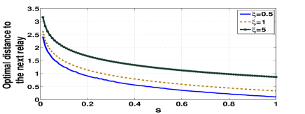
Figure 5: $\beta=1$, $\Lambda:=\frac{\rho}{\beta}=2$; $a^{*}$ vs. $s$.

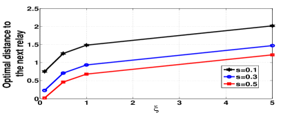
Figure 6: $\beta=1$, $\Lambda:=\frac{\rho}{\beta\texttimes}=2$; $a^{*}$ vs. $\xi$.

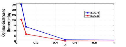
Figure 7: $\beta=1$, $\xi=0.01$; $a^{*}$ vs. $\Lambda$.

Let us recall that the state of the system after placing the $k$-th relay is given by $s_{k}=\frac{e^{\Lambda\tilde{z}_{k}}}{\sum_{i=0}^{k}e^{\Lambda\tilde{z}_{i}}}$. The action is the normalized distance of the next relay to be placed from the current location. The single stage cost function for our total cost minimization problem is given by (14).

In our numerical work, we discretized the state space $(0,1]$ into $100$ steps as $\{0.01,0.02,\cdots,0.99,1\}$, and discretized the action space into steps of size $0.001$, i.e., the action space becomes $\{0,0.001,0.002,\cdots\}$.

5.1 Structure of the Optimal Policy

We performed numerical experiments to study the structure of the optimal policy obtained through value iteration for $\beta=1$ and some values of $\Lambda:=\frac{\rho}{\beta}$. The value iteration in these experiments converged and we obtained a stationary optimal policy, though Theorem 7 does not guarantee the uniqueness of the stationary optimal policy.

Figure 5 shows that the normalized optimal placement distance $a^{*}$ is decreasing with the state $s\in(0,1]$. This can be understood as follows. The state $s$ (at a placement point) is small only if a sufficiently large number of relays have already been placed. Hence, if several relays have already been placed and $\sum_{i=0}^{k}e^{\Lambda\tilde{z}_{i}}$ is sufficiently large compared to $e^{\Lambda\tilde{z}_{k}}$ (i.e., $s_{k}$ is small), the $(k+1)$-st relay will be able to receive sufficient amount of power from the previous nodes, and hence does not need to be placed close to the $k$-th relay. A value of $s_{k}$ close to $1$ indicates that there is a large gap between relay $k$ and relay $k-1$, the power received at the next relay from the previous relays is small and hence the next relay must be placed closer to the previous one.

On the other hand, $a^{*}$ is increasing with $\xi$ (see Figure 6). Recall that $\xi$ is the price of placing a relay. This figure confirms the intuition that if the relay price is high, then the relays should be placed less frequently.

Table I: Sequential placement on a line of length $10$ for various $\Lambda$, using the corresponding optimal policies for $\xi=0.001$.

$\mathbf{\Lambda}$	Normalised Optimal distances of the nodes	No. of
	from the source	relays
$0.01$	0, 0, 8.4180, 10.0000	3
$0.1$	0, 0, 0, 0, 0, 0, 0, 0.2950, 0.5950, 0.9810, 1.3670,	33
	1.7530, 2.1390, $\cdots,$ 9.0870, 9.4730, 9.8590, 10.0000
$5$	0, 0, 0, 0, 0, 0, 0, 0, 0, 0, 0.0020, 0.0080, 0.0140,	1677
	0.0200, $\cdots$, 9.9860, 9.9920, 9.9980, 10.0000

Table II: Evolution of state in the process of sequential placement on a line of length $10$ for various values of $\Lambda$, using the corresponding optimal policies for $\xi=0.001$.

$\mathbf{\Lambda}$	Evolution of state in the process of sequential placement
$0.01$	1, 0.5, 0.34, 0.27
$0.1$	1, 0.5, 0.34, 0.26, 0.21, 0.18, 0.16, 0.14, 0.13, 0.12, 0.12, $\cdots$
$5$	1, 0.5, 0.34, 0.26, 0.21, 0.18, 0.16, 0.14, 0.13, 0.12,
	0.11, 0.1, 0.1, 0.1, $\cdots$

Table III: Sequential placement on a line of length $10$ for various $\Lambda$, using the corresponding optimal policies for $\xi=0.1$.

$\mathbf{\Lambda}$	Normalised Optimal distances of the nodes	No. of
	from the source	relays
$0.01$	10	0
$0.1$	5.3060, 10.0000	1
$5$	0, 0.0050, 0.0510, 0.1220, 0.1930,	143
	0.2640,$\cdots$, 9.9910, 10.0000
$8$	0, 0.003, 0.019, 0.06, 0.101, $\cdots$, 9.982, 10	246
$20$	0, 0.001, 0.003, 0.016, 0.031, 0.046, $\cdots$, 9.991, 10	669

Table IV: Evolution of state in the process of sequential placement on a line of length $10$ for various values of $\Lambda$, using the corresponding optimal policies for $\xi=0.1$.

$\mathbf{\Lambda}$	Evolution of state in the process of sequential placement
$0.01$	1
$0.1$	1, 0.63
$5$	1, 0.5, 0.34, 0.3, 0.3, $\cdots$
$8$	1, 0.5, 0.34, 0.28, 0.28, $\cdots$
$20$	1, 0.5, 0.34, 0.27, 0.26, 0.26, $\cdots$

Figure 7 shows that $a^{*}$ is decreasing with $\Lambda$, for fixed values of $\xi$ and $s$. This happens because increased attenuation will require frequent placement of the relays.

5.2 Relay Placement Patterns

The policy that we use corresponds to a line having exponentially distributed length with mean $1$, but it is applied to the scenario where the actual realization of the (normalised) length (see Section 4.6) of the line is $10$.

Tables I, III, and V illustrate some examples of as-you-go placement of relay nodes along a line of normalised length $10$, using various values of $\Lambda$ and $\xi$. Tables II, IV, and VI illustrate the corresponding evolution of state as the relays are placed in the examples in Tables I, III and V. If the line actually ends at some point before (normalised) distance $10$, the process would end there with the corresponding placement of relays (as can be obtained from Tables I, III, and V) before the sink being placed at the end-point. Thus, for example, reading from Table III for $\xi=0.1$ and $\Lambda=5$, if the actual normalised length of the line is $0.99$, then one relay will be placed at $0$ (the source itself), followed by $15$ relays at normalised distances $0.005,0.051,0.122,0.193,0.264,\cdots,0.974$ from the source, and finally the sink is placed at a normalised distance $0.99$, the end of the line.

We observe that as $\Lambda$ increases, more relays need to be placed since the optimal control decreases with $\Lambda$ for each $s$ (see Figure 7). On the other hand, the number of relays decreases with increasing $\xi$ (the relay cost); this is in confirmation of the observations from Figure 6.

Note that, initially one or more relays are placed at or near the source if $a^{*}(s=1)$ is $0$ or small. But, after some relays have been placed, the relays are placed equally spaced apart. We see that this happens because, after a few relays have been placed, the state, $s$, does not change, hence, resulting in the relays being subsequently placed equally spaced apart. This phenomenon is evident in Table II, Table IV, Table VI, and Figure 8. The state $s$ will remain unchanged after a relay placement if $s=\lceil{\frac{se^{\Lambda a^{*}(s)}}{0.01(1+se^{\Lambda a^{*}(s)})\texttimes}}\rceil\times 0.01$, since we have discretized the state space. After some relays are placed, the state becomes equal to a fixed point $s^{\prime}$ of the function $\lceil{\frac{se^{\Lambda a^{*}(s)}}{0.01(1+se^{\Lambda a^{*}(s)})\texttimes}}\rceil\times 0.01$. Note that the deployment starts from $s_{0}:=1$, but for any value of $s_{0}$ (even with $s_{0}$ smaller than $s^{\prime}$), we numerically observe the same phenomenon. Hence, $s^{\prime}$ is an absorbing state.

Table V: Sequential placement on a line of length $10$ for of $\xi$, using the corresponding optimal policies for $\Lambda=20$.

$\xi$	Normalised Optimal distances of the nodes	No. of
	from the source	relays
$0.2$	0 , 0.008, 0.03, 0.052, $\cdots$, 9.996, 10	456
$1$	0.022, 0.069, 0.116, $\cdots$, 9.986, 10	213
$2$	0.042, 0.103, 0.163, 0.223, $\cdots$, 9.943, 10	166
$10$	0.099, 0.205, 0.311, $\cdots$, 9.957, 10	94

Table VI: Evolution of state in the process of sequential placement on a line of length $10$ for various values of $\xi$, using the corresponding optimal policies for $\Lambda=20$.

$\xi$	Evolution of state in the process of sequential placement
$0.2$	1, 0.5, 0.37, 0.37, $\cdots$
$1$	1, 0.61, 0.61, $\cdots$
$2$	1, 0.7, 0.71, 0.71, $\cdots$
$10$	1, 0.88, 0.88, $\cdots$

5.3 Numerical Examples for Practical Deployment

In order to provide a more concrete illustration we adopt a path loss parameter from [24]. Figure $4$ of [24] shows that the attenuation in the received signal power in a dense urban environment is roughly $50$ dB when we move from $50$ m distance to $300$ m distance away from the transmitter. This yields a value of $\rho$ to be $0.04$ per meter for the exponential path-loss (see the discussion in Section 6.1 on the motivation for choosing the exponential path-loss model in the light of the results from [24]). Then, $\frac{1}{\beta}=200$ m corresponds to $\Lambda=8$, and $\frac{1}{\beta}=500$ m corresponds to $\Lambda=20$. For $\Lambda=20$, normalised relay locations and state evolution $\{s_{k}\}_{k\geq 1}$ are available in Tables III-VI, and, for $\Lambda=8$, normalised relay locations and state evolution $\{s_{k}\}_{k\geq 1}$ are available in Tables III-IV. Note that, under $\rho=0.04$ per meter and $\Lambda=20$, one unit normalised distance in the tables correspond to $500$ m distance in the dense urban environment (due to the normalization as in Section 4.6).

For the sake of illustration, let us consider the sample deployment for $\xi=10$, $\Lambda=20$ (Table V). In this case, the first relay will be placed at a distance $0.099\times 500=49.5$ m from the source, the second relay will be placed at a distance $0.205\times 500=102.5$ m from the source, etc. Also, if we choose $\xi$ such that few relays will be placed on a typical line whose length is several hundreds of meters, then the relays will be placed almost uniformly on the line. But, for small $\xi$, more relays will be placed and some of them will be clustered near the source (see the deployment for $\Lambda=8$ and $\xi=0.1$ in Table III).

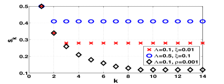
Figure 8: Evolution of the state $s_{k}$ with $k$: initial state $s_{0}=1$.

Table VII: Comparison of the performance (in terms of $H$; see text) of optimal sequential placement over a line of random length, with the optimal placement if the length was known. Results from 10000 samples of exponentially distributed line lengths.

		Average	Mean	Number of	Maximum
$\xi$	$\Lambda$	percentage	number of	cases where	percentage
		difference	relays used	no relay	difference
				was used
0.001	0.01	0.0068	2.0002	0	0.7698
0.001	0.1	0.3996	9.4849	0	6.8947
0.01	0.01	0	0	10000	0
0.01	0.1	0.3517	2.2723	0	4.6618
0.01	0.5	1.5661	7.7572	0	4.7789
0.1	0.01	0	0	10000	0
0.1	0.1	0.1259	0.0056	9944	25.9098
0.1	0.5	2.9869	1.8252	0	12.5907
0.1	2	4.7023	7.1530	0	9.0211
0.1	20	3.5472	27.9217	0	6.6223
0.1	8	4.0097	21.0671	0	7.8264
1	8	8.0286	7.8886	495	27.7362
1	20	5.2158	11.2342	402	26.0026
5	20	10.3341	7.1950	597	61.7460

5.4 Comparison with Optimal Offline Deployment

Since there is no prior work in the literature with which we can make a fair comparison of our as-you-go deployment policy for the full-duplex wireless multi-relay network, we compare the performance of our policy with optimal offline deployment. Thus, the numerical experiments reported in Table VII are a result of asking the following question: how does the cost of as-you-go deployment over a line of exponentially distributed length compare with the cost of placing the same number of relays optimally over the line, once the length of the line has been revealed?

For several combinations of $\Lambda$ and $\xi$, we generated $10000$ random numbers independently from an exponential distribution with parameter $\beta=1$. Each of these numbers was considered as a possible realization of the length of the line. Then we computed the placement of the relay nodes for each realization by optimal sequential placement policy, which gave us $H=\frac{1}{g_{0,1}\texttimes}+\sum_{k=2}^{N+1}\frac{(g_{0,k-1}-g_{0,k})}{g_{0,k}g_{0,k-1}\sum_{l=0}^{k-1}\frac{1}{g_{0,l}\texttimes}\texttimes}$, a quantity that we use to evaluate the quality of the relay placement. The significance of $H$ can be recalled from (6) where we found that the rate $C(1+\frac{P_{T}/\sigma^{2}}{H})$ can be achieved if total power $P_{T}$ is available to distribute among the source and the relays; i.e., $H$ can be interpreted as the net effective attenuation after power has been allocated optimally over the nodes. Also, for each realization, we computed $H$ for optimal relay placement, assuming that the length of the line is known before deployment and that the number of relays available is the same as the number of relays used by the corresponding sequential placement policy. For a given combination of $\Lambda$ and $\xi$, for the $k$-th realization of the length of the line, let us denote the two $H$ values by $H_{\mathsf{sequential}}^{(k)}$ and $H_{\mathsf{optimal}}^{(k)}$. Then the percentage difference for the $k$-th realization is:

$$e_{k}:=\frac{|H_{\mathsf{optimal}}^{(k)}-H_{\mathsf{sequential}}^{(k)}|}{H_{\mathsf{optimal}}^{(k)}}\times 100$$ (23)

The average percentage difference in Table VII is the quantity $\frac{\sum_{k=1}^{10000}e_{k}}{10000\texttimes}$. The maximum percentage difference is the quantity $\max_{k\in\{1,2,\cdots,10000\}}e_{k}$.

Discussion of Table VII:

1. For small enough $\xi$, some relays will be placed at the source itself. For example, for $\Lambda=0.01$ and $\xi=0.001$, we will place two relays at the source (Table I). After placing the first relay, the next state will become $s=0.5$, and $a^{*}(s=0.5)=0$. The state after placing the second relay becomes $s=0.34$, for which $a^{*}(s=0.34)=8.41$ (see the placement in Table I). Now, the line having an exponentially distributed length with mean $1$ will end before $a^{*}(s=0.34)=8.41$ distance with high probability, and the probability of placing the third relay will be very small. As a result, the mean number of relays will be $2.0002$. In case only $2$ relays are placed by the sequential deployment policy and we seek to place $2$ relays optimally for the same length of the line (with the length known), the optimal locations for both relays are close to the source location if the length of the line is small (i.e., if the attenuation $\lambda$ is small, recall the definition of $\lambda$ from Section 3.2). If the line is long (which has a very small probability), the optimal placement will be significantly different from the sequential placement. Altogether, the difference (from (23)) will be small.

2. For $\Lambda=0.01$ and $\xi=0.1$, $a^{*}(1)$ is so large that with high probability the line will end in a distance less than $a^{*}(1)$ and no relay will be placed.

3. From (6) we know that for a given placement of relays on a line of given length $L$, the optimal power allocation yields an achievable rate $\log_{2}(1+\frac{P_{T}/\sigma^{2}}{H})$. At the end of as-you-go deployment the power is allocated optimally among the nodes deployed, and a rate $\log_{2}(1+\frac{P_{T}/\sigma^{2}}{H_{sequential}})$ can be achieved. If the same number of relays are optimally placed over the same line, with the same total power, then the inner bound is given by $\log_{2}(1+\frac{P_{T}/\sigma^{2}}{H_{optimal}})$. We seek to compare these two rates numerically.

   The maximum fractional difference in Table VII is less than $\frac{2}{3}$, and substantially smaller than $\frac{2}{3}$ in most cases. Since, in (23), $H_{sequential}^{(k)}$ is always greater than $H_{optimal}^{(k)}$, we have $H_{sequential}^{(k)}\leq\frac{5}{3}H_{optimal}^{(k)}$ for all $k\geq 1$ (i.e., for all realizations of $L$ in the simulation). Now, by the monotonicity of $\log_{2}(\cdot)$:

   $$\frac{1}{2}\log_{2}\bigg{(}1+\frac{P_{T}/\sigma^{2}}{H_{optimal}^{(k)}}\bigg{)}-\frac{1}{2}\log_{2}\bigg{(}1+\frac{P_{T}/\sigma^{2}}{H_{sequential}^{(k)}}\bigg{)}$$

   $$\leq \frac{1}{2}\log_{2}\bigg{(}1+\frac{P_{T}/\sigma^{2}}{H_{optimal}^{(k)}}\bigg{)}-\frac{1}{2}\log_{2}\bigg{(}1+\frac{P_{T}/\sigma^{2}}{\frac{5}{3}H_{optimal}^{(k)}}\bigg{)}$$

   Since $\log_{2}(\cdot)$ is a concave function, for any $x>y>0$, we have $\log_{2}(1+x)-\log_{2}(1+y)\leq\log_{2}(x)-\log_{2}(y)$. Using this inequality, we can upper bound the difference in achievable rate from the previous equation by:

   $$\frac{1}{2}\log_{2}\bigg{(}\frac{P_{T}/\sigma^{2}}{H_{optimal}^{(k)}}\bigg{)}-\frac{1}{2}\log_{2}\bigg{(}\frac{P_{T}/\sigma^{2}}{\frac{5}{3}H_{optimal}^{(k)}}\bigg{)}=0.3685$$

   This calculation implies that, for the large number of cases reported in Table VII, by using the approximation in (10) and by using the corresponding optimal policy for as-you-go deployment, we lose at most $0.3685$ bits per channel use, compared to the case when the realization of the exponentially distributed source to sink distance is known apriori and when we use the same number of relays as used in the as-you-go deployment case. Note that, the statement of this claim holds with high probability since the maximum difference is taken over $10000$ sample deployments. Hence, it is reasonable to solve (10) instead of (11) which is intractable.

6 Discussion

6.1 Exponential Path-Loss Model

Exponential path-loss model has been used before in the context of relay placement (see [16], [22]) and in the context of cellular networks (see [26, Section $2.3$]). Analytical and experimental support for the exponential path-loss model have been provided by Franceschetti et al. ([24]). Franceschetti et al. used a random scattering model (applicable to an urban environment, or a forest environment) to show that the path-loss in such an environment is the product of an exponential function and a power function of the distance (see [24, Equation $(14)$]). Figure $4$ of their paper, which is obtained from measurements made in an urban environment, shows that path-loss (in dB) varies linearly with distance beyond a distance of $40-50$ meters, which implies exponential path-loss for longer distance. These distances are practical for urban scenarios where the network is deployed over several hundreds of meters or several kilometers.

Exponential path-loss was also proposed by Marano and Franceschetti for urban environment, and validated by theory and experiment (see [30, Figure $10$]).

6.2 Incorporating Shadowing and Fading

Shadowing (which is typically viewed as being static once a link is deployed) and time varying fading, can be incorporated in our setting by providing a fade-margin in the power at each transmitter. Thus, when expressed in dBm, the actual transmit power for any transmitter-receiver pair is the fade-margin plus the power used in the information theoretic capacity formulas; this fade-margin does not depend on the distance between the transmitter-receiver pair. Note that, this approach, though very conservative in nature, can remove the complexity in analysis arising out of fading in the network. Also note that, if the actual power gain between two nodes $r$ distance apart is $c_{0}e^{-\rho r}$ with $c_{0}>0$, then $c_{0}$ can be absorbed in the fade margin.

6.3 Full-Duplex Decode-and-Forward Relaying

Full-duplex radios might become a reality soon; see [11], [12], [13], [14] for recent efforts to realize them. Decode-and-forward relaying requires symbol-level synchronous operation across all nodes in the network. The requirement of globally coherent transmission and reception seems to be restrictive at the moment, but this problem will be solved with the advent of better clocks (with less drift) and efficient clock synchronization algorithms. Any research on impromptu deployment assuming imperfect synchronization, or half-duplex communication, or no interference cancellation, can use this paper as a benchmark for performance analysis.

6.4 Insights on Power-Law Path-Loss

In [1], we studied the problem of single-relay placement under a per-node power constraint at the source and the relay, for both exponential and power-law path-loss models. The variation of optimal relay location, as the amount of attenuation in the network varies, follow slightly different (but mostly similar) trends (see Figures $2$ and $3$ of [1]) because of the fact that power-law model allows unbounded power gain (unlike the exponential model) when the distance $r$ tends to $0$ ($\lim_{r\rightarrow 0}r^{-\eta}=\infty$). The findings are even more similar when we bound the power gain from above by some constant value in case of the power-law model (power gain is $\min\{r^{-\eta},b^{-\eta}\}$ for some $b>0$); see the similarity between Figures $2$ and $4$ in [1]. The results on the fixed node power case provide the insight that when the power gain is $r^{-\eta}$ or $\min\{r^{-\eta},b^{-\eta}\}$; under the sum power constraint, the variation of the relay locations as a function of attenuation will follow a pattern similar to that in case of exponential path-loss.

7 Conclusion

Motivated by the problem of as-you-go deployment of wireless relay networks, we first studied the problem of placing relay nodes along a line, in order to connect a sink at the end of the line to a source at the start of the line, so as to maximize the end-to-end achievable data rate. For the multi-relay channel with exponential path-loss and sum power constraint, we derived an expression for the achievable rate in terms of the power gains among all possible node pairs, and formulated an optimization problem in order to maximize the end-to-end data rate. Numerical work for the fixed source-sink distance suggests that at low attenuation the relays are mostly clustered close to the source in order to be able to cooperate among themselves, whereas at high attenuation they are uniformly placed and work as repeaters. Next, the deploy-as-you-go sequential placement problem was addressed; a sequential relay placement problem along a line having unknown random length was formulated as an MDP, the value function was characterized analytically, and the policy structure was investigated numerically. We found numerically that at the initial stage of the deployment process the inter-relay distances are smaller, and, as deployment progresses, the inter-relay distances increase gradually, and finally the relays start being placed at regular intervals.

Our results are based on information theoretic achievable rate results. In order to utilize currently commercially available wireless devices, we have also been exploring non-information theoretic, packet forwarding models for optimal relay placement, with the aim of obtaining placement algorithms that can be easily reduced to practice (see [7] for reference). The study of as-you-go deployment under the information theoretic model and under the packet forwarding model provides two complementary approaches for two different conditions in the physical layer and the MAC layer, and provides a more comprehensive development of the problem.

Arpan Chattopadhyay obtained his B.E. in Electronics and Telecommunication Engineering from Jadavpur University, Kolkata, India in the year 2008, and M.E. and Ph.D in Telecommunication Engineering from Indian Institute of Science, Bangalore, India in the year 2010 and 2015, respectively. He is currently working in INRIA, Paris as a postdoctoral researcher. His research interests include networks and machine learning.

Abhishek Sinha is currently a graduate student in the Laboratory for Information and Decision Systems (LIDS), at Massachusetts Institute of Technology, Cambridge, MA. Prior to joining MIT, he completed his Master’s studies in Telecommunication Engineering at the Indian Institute of Science, Bangalore, in the year 2012. His areas of interests include stochastic processes, information theory and network control.

Marceau Coupechoux is an Associate Professor at Telecom ParisTech since 2005. He obtained his master from Telecom ParisTech in 1999 and from University of Stuttgart, Germany in 2000, and his Ph.D. from Institut Eurecom, Sophia-Antipolis, France, in 2004. From 2000 to 2005, he was with Alcatel-Lucent (Bell Labs former Research & Innovation and then in the Network Design department). In the Computer and Network Science department of Telecom ParisTech, he is working on cellular networks, wireless networks, ad hoc networks, cognitive networks, focusing mainly on layer 2 protocols, scheduling and resource management. From August 2011 to August 2012 he was a visiting scientist at IISc Bangalore.

Anurag Kumar obtained his B.Tech. degree from the Indian Institute of Technology at Kanpur, and the PhD degree from Cornell University, both in Electrical Engineering. He was then with Bell Laboratories, Holmdel, N.J., for over 6 years. Since 1988 he has been on the faculty of the Indian Institute of Science (IISc), Bangalore, in the Department of Electrical Communication Engineering. He is currently also the Director of the Institute. From 1988 to 2003 he was the Coordinator at IISc of the Education and Research Network Project (ERNET), India’s first wide-area packet switching network. His area of research is communication networking, specifically, modeling, analysis, control and optimisation problems arising in communication networks and distributed systems. Recently his research has focused primarily on wireless networking. He is a Fellow of the IEEE, of the Indian National Science Academy (INSA), of the Indian Academy of Science (IASc), of the Indian National Academy of Engineering (INAE), and of The World Academy of Sciences (TWAS). He is a recepient of the Indian Institute of Science Alumni Award for Engineering Research for 2008.

Appendix A A Brief Description of the Coding Scheme of [10]

Transmissions take place via block codes of $T$ symbols each. The transmission blocks at the source and the $N$ relays are synchronized. The coding and decoding scheme is such that a message generated at the source at the beginning of block $b,b\geq 1,$ is decoded by the sink at the end of block $b+N$, i.e., $N+1$ block durations after the message was generated (with probability tending to 1, as $T\to\infty)$. Thus, at the end of $B$ blocks, $B\geq N+1$, the sink is able to decode $B-N$ messages. It follows, by taking $B\to\infty$, that, if the code rate is $R$ bits per symbol, then an information rate of $R$ bits per symbol can be achieved from the source to the sink.

As mentioned earlier, we index the source by $0$, the relays by $k,1\leq k\leq N$, and the sink by $N+1$. There are $(N+1)^{2}$ independent Gaussian random codebooks, each containing $2^{TR}$ codes, each code being of length $T$; these codebooks are available to all nodes. At the beginning of block $b$, the source generates a new message $w_{b}$, and, at this stage, we assume that each node $k,1\leq k\leq N+1,$ has a reliable estimate of all the messages $w_{b-j},j\geq k$. In block $b$, the source uses a new codebook to encode $w_{b}$. In addition, relay $k,1\leq k\leq N,$ and all of its previous transmitters (indexed $0\leq j\leq k-1$), use another codebook to encode $w_{b-k}$ (or their estimate of it). Thus, if the relays $1,2,\cdots,k$ have a perfect estimate of $w_{b-k}$ at the beginning of block $b$, they will transmit the same codeword for $w_{b-k}$. Therefore, in block $b$, the source and relays $1,2,\cdots,k$ coherently transmit the codeword for $w_{b-k}$. In this manner, in block $b$, transmitter $k,0\leq k\leq N,$ generates $N+1-k$ codewords, corresponding to $w_{b-k},w_{b-k-1},\cdots,w_{b-N}$, which are transmitted with powers $P_{k,k+1},P_{k,k+2},\cdots,P_{k,N+1}$. In block $b$, node $k,1\leq k\leq N+1,$ receives a superposition of transmissions from all other nodes. Assuming that node $k$ knows all the powers, and all the channel gains, and recalling that it has a reliable estimate of all the messages $w_{b-j},j\geq k$, it can subtract the interference from transmitters $k+1,k+2,\cdots,N$. At the end of block $b$, after subtracting the signals it knows, node $k$ is left with the $k$ received signals from nodes $0,1,\cdots,(k-1)$ (received in blocks $b,b-1,\cdots,b-k+1$), which all carry an encoding of the message $w_{b-k+1}$. These $k$ signals are then jointly used to decode $w_{b-k+1},$ using joint typicality decoding. The codebooks are cycled through in a manner so that in any block all nodes encoding a message (or their estimate of it) use the same codebook, but different (thus, independent) codebooks are used for different messages. Under this encoding and decoding scheme, any rate strictly less than $R$ displayed in (2) is achievable.

Appendix B Proof of Theorem 1

We want to maximize $R$ given in (2) subject to the total power constraint, assuming fixed relay locations. Let us consider $C(\frac{1}{\sigma^{2}\texttimes}\sum_{j=1}^{k}(\sum_{i=0}^{j-1}h_{i,k}\sqrt{P_{i,j}})^{2})$, i.e., the $k$-th term in the argument of $\min\{\cdots\}$ in (2). By the monotonicity of $C(\cdot)$, it is sufficient to consider $\sum_{j=1}^{k}(\sum_{i=0}^{j-1}h_{i,k}\sqrt{P_{i,j}})^{2}$. Now since the channel gains are multiplicative, we have:

$$\sum_{j=1}^{k}(\sum_{i=0}^{j-1}h_{i,k}\sqrt{P_{i,j}})^{2}=g_{0,k}\sum_{j=1}^{k}\bigg{(}\sum_{i=0}^{j-1}\frac{\sqrt{P_{i,j}}}{h_{0,i}\texttimes}\bigg{)}^{2}$$

Thus our optimization problem becomes:

$$\max\,\min_{k\in\{1,2,\cdots,N+1\}}g_{0,k}\sum_{j=1}^{k}\bigg{(}\sum_{i=0}^{j-1}\frac{\sqrt{P_{i,j}}}{h_{0,i}\texttimes}\bigg{)}^{2}$$ (24)

s.t $$\,\sum_{j=1}^{N+1}\gamma_{j}\leq P_{T}\,\,\textit{and}\,\sum_{i=0}^{j-1}P_{i,j}=\gamma_{j}\,\forall\,1\leq j\leq(N+1)$$

Let us fix $\gamma_{1},\gamma_{2},\cdots,\gamma_{N+1}$ such that their sum is equal to $P_{T}$. We observe that $P_{i,N+1}$ for $i\in\{0,1,\cdots,N\}$ appear in the objective function only once: for $k=N+1$ through the term $(\sum_{i=0}^{N}\frac{\sqrt{P_{i,N+1}}}{h_{0,i}\texttimes})^{2}$. Since we have fixed $\gamma_{N+1}$, we need to maximize this term over $P_{i,N+1},\,i\in\{0,1,\cdots,N\}$. So we have the following optimization problem:

$$\max\sum_{i=0}^{N}\frac{\sqrt{P_{i,N+1}}}{h_{0,i}\texttimes}\,\,\,\,\,\textit{s.t}\,\,\,\,\,\sum_{i=0}^{N}P_{i,N+1}=\gamma_{N+1}$$ (25)

By Cauchy-Schwartz inequality, the objective function in this optimization problem is upper bounded by (using the fact that $g_{0,i}=h_{0,i}^{2}$ $\forall i\in\{0,1,\cdots,N\}$):

$$\sqrt{(\sum_{i=0}^{N}P_{i,N+1})(\sum_{i=0}^{N}\frac{1}{g_{0,i}\texttimes})}=\sqrt{\gamma_{N+1}\sum_{i=0}^{N}\frac{1}{g_{0,i}}}$$

The upper bound is achieved if there exists some $c>0$ such that $\frac{\sqrt{P_{i,N+1}}}{\frac{1}{h_{0,i}\texttimes}\texttimes}=c$ $\forall i\in\{0,1,\cdots,N\}$. So we have:

$$P_{i,N+1}=\frac{c^{2}}{g_{0,i}\texttimes}\,\,\forall i\in\{0,1,\cdots,N\}\\$$

Since $\sum_{i=0}^{N}P_{i,N+1}=\gamma_{N+1}$, we obtain $c^{2}=\frac{\gamma_{N+1}}{\sum_{l=0}^{N}\frac{1}{g_{0,l}\texttimes}\texttimes}$. Thus, $P_{i,N+1}=\frac{\frac{1}{g_{0,i}\texttimes}}{\sum_{l=0}^{N}\frac{1}{g_{0,l}\texttimes}\texttimes}\gamma_{N+1}$.

Here we have used the fact that $h_{0,0}=1$. Now $\{P_{i,N}:i=0,1,\cdots,(N-1)\}$ appear only through the sum $\sum_{i=0}^{N-1}\frac{\sqrt{P_{i,N}}}{h_{0,i}\texttimes}$, and it appears twice: for $k=N$ and $k=N+1$. We need to maximize this sum subject to the constraint $\sum_{i=0}^{N-1}P_{i,N}=\gamma_{N}$. This optimization can be solved in a similar way as before. Thus by repeatedly using this argument and solving optimization problems similar in nature to (25), we obtain:

$$P_{i,j}=\frac{\frac{1}{g_{0,i}\texttimes}}{\sum_{l=0}^{j-1}\frac{1}{g_{0,l}\texttimes}\texttimes}\gamma_{j}\,\,\forall 0\leq i<j\leq(N+1)$$ (26)

Substituting for $P_{i,j},0\leq i<j\leq(N+1)$ in (24), we obtain the following optimization problem:

$$\max\min_{k\in\{1,2,\cdots,N+1\}}g_{0,k}\sum_{j=1}^{k}\bigg{(}\gamma_{j}\sum_{i=0}^{j-1}\frac{1}{g_{0,i}\texttimes}\bigg{)}$$ (27)

s.t. $$\,\,\sum_{j=1}^{N+1}\gamma_{j}\leq P_{T}$$

Let us define $b_{k}:=g_{0,k}$ and $a_{j}:=\sum_{i=0}^{j-1}\frac{1}{g_{0,i}\texttimes}$. Observe that $b_{k}$ is decreasing and $a_{k}$ is increasing with $k$. Let us define:

$$\tilde{s}_{k}(\gamma_{1},\gamma_{2},\cdots,\gamma_{N+1}):=b_{k}\sum_{j=1}^{k}a_{j}\gamma_{j}$$ (28)

With this notation, our optimization problem becomes:

$$\max\min_{1\leq k\leq N+1}\tilde{s}_{k}(\gamma_{1},\gamma_{2},\cdots,\gamma_{N+1})\,\,\,\,\textit{s.t.}\,\,\sum_{j=1}^{N+1}\gamma_{j}\leq P_{T}$$ (29)

Claim 1

Under optimal allocation of $\gamma_{1},\gamma_{2},\cdots,\gamma_{N+1}$ for the optimization problem (29), $\tilde{s}_{1}=\tilde{s}_{2}=\cdots=\tilde{s}_{N+1}$. ∎

Proof:

(29) can be rewritten as:

$$\max\zeta$$

s.t $$\zeta\leq b_{k}\sum_{j=1}^{k}a_{j}\gamma_{j}\,\forall\,k\in\{1,2,\cdots,N+1\},$$ (30)

$$\sum_{j=1}^{N+1}\gamma_{j}\leq P_{T},\,\,\,\gamma_{j}\geq 0\,\,\forall\,1\leq j\leq N+1$$

The dual of this linear program is given by:

$$\min P_{T}\theta$$

s.t $$\sum_{k=1}^{N+1}\mu_{k}=1,\,\,\,\theta\geq 0,$$ (31)

$$a_{l}\sum_{k=l}^{N+1}b_{k}\mu_{k}+\nu_{l}=\theta\,\forall\,l\in\{1,2,\cdots,N+1\},$$

$$\mu_{l}\geq 0,\nu_{l}\geq 0\,\forall\,l\in\{1,2,\cdots,N+1\}$$

Now, let us consider a primal feasible solution $(\{\gamma_{j}^{*}\}_{1\leq j\leq N+1},\zeta^{*})$ which satisfies:

$$b_{k}\sum_{j=1}^{k}a_{j}\gamma_{j}^{*}=\zeta^{*}\,\forall\,k\in\{1,2,\cdots,N+1\},$$

$$\sum_{j=1}^{N+1}\gamma_{j}^{*}=P_{T}$$ (32)

Thus we have, $b_{1}a_{1}\gamma_{1}^{*}=\zeta^{*}$, i.e., $\gamma_{1}^{*}=\frac{\zeta^{*}}{b_{1}a_{1}\texttimes}$. Again, $b_{2}(a_{1}\gamma_{1}^{*}+a_{2}\gamma_{2}^{*})=\zeta^{*}$, which implies $\frac{b_{2}}{b_{1}\texttimes}\zeta^{*}+b_{2}a_{2}\gamma_{2}^{*}=\zeta^{*}$.

Thus we obtain $\gamma_{2}^{*}=\frac{\zeta^{*}}{a_{2}\texttimes}(\frac{1}{b_{2}\texttimes}-\frac{1}{b_{1}\texttimes})$. In general, we can write:

$$\gamma_{k}^{*}=\frac{\zeta^{*}}{a_{k}\texttimes}\left(\frac{1}{b_{k}\texttimes}-\frac{1}{b_{k-1}\texttimes}\right)\,\forall k\in\{1,2,\cdots,N+1\}\\$$

with $\frac{1}{b_{0}\texttimes}:=0$. Now, since $\sum_{k=1}^{N+1}\gamma_{k}^{*}=P_{T}$, we obtain:

$$\zeta^{*} = \frac{P_{T}}{\sum_{k=1}^{N+1}\frac{1}{a_{k}\texttimes}(\frac{1}{b_{k}\texttimes}-\frac{1}{b_{k-1}\texttimes})\texttimes}$$

$$\gamma_{j}^{*} = \frac{\frac{1}{a_{j}\texttimes}\left(\frac{1}{b_{j}\texttimes}-\frac{1}{b_{j-1}\texttimes}\right)}{\sum_{k=1}^{N+1}\frac{1}{a_{k}\texttimes}(\frac{1}{b_{k}\texttimes}-\frac{1}{b_{k-1}\texttimes})\texttimes}P_{T},\,j\in\{1,2,\cdots,N+1\}$$ (33)

It should be noted that since $b_{k}$ is nonincreasing in $k$, the primal variables above are nonnegative and satisfies feasibility conditions. Again, let us consider a dual feasible solution $(\{\mu_{j}^{*},\nu_{j}^{*}\}_{1\leq j\leq N+1},\theta^{*})$ which satisfies:

$$\sum_{k=1}^{N+1}\mu_{k}^{*}=1,\,\,\,\nu_{l}^{*}=0\,\forall\,l\in\{1,2,\cdots,N+1\}$$

$$a_{l}\sum_{k=l}^{N+1}b_{k}\mu_{k}^{*}+\nu_{l}^{*}=\theta^{*}\,\forall\,l\in\{1,2,\cdots,N+1\}$$ (34)

Solving these equations, we obtain:

$$\theta^{*} = \frac{1}{\sum_{k=1}^{N+1}\frac{1}{b_{k}\texttimes}\left(\frac{1}{a_{k}\texttimes}-\frac{1}{a_{k+1}\texttimes}\right)\texttimes}$$

$$\mu_{j}^{*} = \frac{\frac{1}{b_{j}\texttimes}(\frac{1}{a_{j}\texttimes}-\frac{1}{a_{j+1}\texttimes})}{\sum_{k=1}^{N+1}\frac{1}{b_{k}\texttimes}\left(\frac{1}{a_{k}\texttimes}-\frac{1}{a_{k+1}\texttimes}\right)\texttimes},\,j\in\{1,2,\cdots,N+1\}$$ (35)

where $\frac{1}{a_{N+2}\texttimes}:=0$. Since $a_{k}$ is increasing in $k$, all dual variables are feasible. It is easy to check that $\zeta^{*}=P_{T}\theta^{*}$, which means that there is no duality gap. Since the primal is a linear program, the solution $(\gamma_{1}^{*},\gamma_{2}^{*},\cdots,\gamma_{N+1}^{*},\zeta^{*})$ is primal optimal. Thus we have established the claim, since the primal optimal solution satisfies it. ∎

So let us obtain $\gamma_{1},\gamma_{2},\cdots,\gamma_{N+1}$ for which $\tilde{s}_{1}=\tilde{s}_{2}=\cdots=\tilde{s}_{N+1}$. Putting $\tilde{s}_{k}=\tilde{s}_{k-1}$, we obtain $b_{k}\sum_{j=1}^{k}a_{j}\gamma_{j}=b_{k-1}\sum_{j=1}^{k-1}a_{j}\gamma_{j}$. Thus, we obtain, $\gamma_{k}=\frac{(b_{k-1}-b_{k})}{b_{k}\texttimes}\frac{1}{a_{k}\texttimes}\sum_{j=1}^{k-1}a_{j}\gamma_{j}$

Let $d_{k}:=\frac{(b_{k-1}-b_{k})}{b_{k}\texttimes}\frac{1}{a_{k}\texttimes}$. Hence, $\gamma_{k}=d_{k}\sum_{j=1}^{k-1}a_{j}\gamma_{j}$. From this recursive equation, we have $\gamma_{2}=d_{2}a_{1}\gamma_{1}$, $\gamma_{3}=d_{3}(a_{1}\gamma_{1}+a_{2}\gamma_{2})=d_{3}a_{1}(1+a_{2}d_{2})\gamma_{1}$, and, in general for $k\geq 3$,

$$\gamma_{k}=d_{k}a_{1}\Pi_{j=2}^{k-1}(1+a_{j}d_{j})\gamma_{1}$$ (36)

Using the fact that $\gamma_{1}+\gamma_{2}+\cdots+\gamma_{N+1}=P_{T}$, we obtain:

$$\gamma_{1}=\frac{P_{T}}{1+d_{2}a_{1}+\sum_{k=3}^{N+1}d_{k}a_{1}\Pi_{j=2}^{k-1}(1+a_{j}d_{j})\texttimes}$$ (37)

Thus if $\tilde{s}_{1}=\tilde{s}_{2}=\cdots=\tilde{s}_{N+1}$, there is a unique allocation $\gamma_{1},\gamma_{2},\cdots,\gamma_{N+1}$. So this must be the one maximizing $R$. Hence, optimum $\gamma_{1}$ is obtained by (37). Then, substituting the values of $\{a_{k}:k=0,1,\cdots,N\}$ and $d_{k}:k=1,2,\cdots,N+1$ in (36) and (37), we obtain the values of $\gamma_{1},\gamma_{2},\cdots,\gamma_{N+1}$ as shown in Theorem 1.

Now under these optimal values of $\gamma_{1},\gamma_{2},\cdots,\gamma_{N+1}$, all terms in the argument of $\min\{\cdots\}$ in (2) are equal. So we can consider the first term alone. Thus we obtain the expression for $R$ optimized over power allocation among all the nodes for fixed relay locations as : $R_{P_{T}}^{opt}(y_{1},y_{2},\cdots,y_{N})=C\left(\frac{g_{0,1}P_{0,1}}{\sigma^{2}\texttimes}\right)=C\left(\frac{g_{0,1}\gamma_{1}}{\sigma^{2}\texttimes}\right)$. Substituting the expression for $\gamma_{1}$ from (5), we obtain the achievable rate formula (6).∎

$$z_{1}^{*}+\frac{z_{2}^{*}-z_{1}^{*}}{1+z_{1}^{*}\texttimes}+\cdots+\frac{e^{\rho y}-z_{i}^{*}}{1+z_{1}^{*}+\cdots+z_{i}^{*}\texttimes}+\frac{z_{i+1}^{*}-e^{\rho y}}{1+z_{1}^{*}+\cdots+z_{i}^{*}+e^{\rho y}\texttimes}+\cdots.+\frac{e^{\rho L}-z_{N}^{*}}{1+z_{1}^{*}+\cdots+z_{i}^{*}+e^{\rho y}+z_{i+1}^{*}+\cdots+z_{N}^{*}\texttimes}$$

$$<z_{1}^{*}+\frac{z_{2}^{*}-z_{1}^{*}}{1+z_{1}^{*}\texttimes}+\cdots+\frac{e^{\rho L}-z_{N}^{*}}{1+z_{1}^{*}+\cdots+z_{i}^{*}+z_{i+1}^{*}+\cdots+z_{N}^{*}\texttimes}$$ (38)

 

Appendix C Proof of Theorem 2

Here we want to place the relay node at a distance $r_{1}$ from the source to minimize $\bigg{\{}\frac{1}{g_{0,1}\texttimes}+\frac{g_{0,1}-g_{0,2}}{g_{0,2}(1+g_{0,1})\texttimes}\bigg{\}}$ (see Equation (6)). Hence, our optimization problem becomes :

$$\min_{r_{1}\in[0,L]}\bigg{\{}e^{\rho r_{1}}+\frac{e^{-\rho r_{1}}-e^{-\rho L}}{e^{-\rho L}(1+e^{-\rho r_{1}})\texttimes}\bigg{\}}\\$$

Writing $z_{1}=e^{\rho r_{1}}$, the problem becomes :

$$\min_{z_{1}\in[1,e^{\rho L}]}\bigg{\{}z_{1}-1+\frac{e^{\rho L}+1}{z_{1}+1\texttimes}\bigg{\}}\\$$

This is a convex optimization problem. Equating the derivative of the objective function to zero, we obtain $1-\frac{e^{\rho L}+1}{(z_{1}+1)^{2}\texttimes}=0$. Thus the derivative becomes zero at $z_{1}^{\prime}=\sqrt{1+e^{\rho L}}-1>0$. Hence, the objective function is decreasing in $z_{1}$ for $z_{1}\leq z_{1}^{\prime}$ and increasing in $z_{1}\geq z_{1}^{\prime}$. So the minimizer is $z_{1}^{*}=\max\{z_{1}^{\prime},1\}$. So the optimum distance of the relay node from the source is $y_{1}^{*}=r_{1}^{*}=\max\{0,r_{1}^{\prime}\}$, where $r_{1}^{\prime}=\frac{1}{\rho\texttimes}\log(\sqrt{1+e^{\rho L}}-1)$. Hence, $\frac{y_{1}^{*}}{L\texttimes}=\max\{\frac{1}{\lambda\texttimes}\log\left(\sqrt{e^{\lambda}+1}-1\right),0\}$. Now $r_{1}^{\prime}\geq 0$ if and only if $\lambda\geq\log 3$. Hence, $\frac{y_{1}^{*}}{L\texttimes}=0$ for $\lambda\leq\log 3$ and $\frac{y_{1}^{*}}{L\texttimes}=\frac{1}{\lambda\texttimes}\log\left(\sqrt{e^{\lambda}+1}-1\right)$ for $\lambda\geq\log 3$.

For $\lambda\leq\log 3$, the relay is placed at the source. Then $g_{0,1}=1$ and $g_{0,2}=g_{1,2}=e^{-\lambda}$. Then $P_{0,1}=\gamma_{1}=\frac{2P_{T}}{e^{\lambda}+1\texttimes}$ (by Theorem $1$) and $R^{*}=C\left(\frac{2P_{T}}{(e^{\lambda}+1)\sigma^{2}\texttimes}\right)$. Also $\gamma_{2}=\frac{e^{\lambda}-1}{e^{\lambda}+1\texttimes}P_{T}$. Hence, $P_{0,2}=P_{1,2}=\frac{e^{\lambda}-1}{e^{\lambda}+1\texttimes}\frac{P_{T}}{2\texttimes}$.

for $\lambda\geq\log 3$, the relay is placed at $r_{1}^{\prime}$. Substituting the value of $r_{1}^{\prime}$ into Equation ($\ref{eqn:power_gamma_relation})$, we obtain $P_{0,1}=\gamma_{1}=\frac{P_{T}}{2\texttimes}$, $P_{0,2}=\frac{1}{\sqrt{e^{\lambda}+1}\texttimes}\frac{P_{T}}{2\texttimes}$, $P_{1,2}=\frac{\sqrt{e^{\lambda}+1}-1}{\sqrt{e^{\lambda}+1}\texttimes}\frac{P_{T}}{2\texttimes}$. So in this case $R^{*}=C\left(\frac{g_{0,1}P_{0,1}}{\sigma^{2}\texttimes}\right)$. Since $P_{0,1}=\frac{P_{T}}{2\texttimes}$, we have $R^{*}=C\left(\frac{1}{\sqrt{e^{\lambda}+1}-1\texttimes}\frac{P_{T}}{2\sigma^{2}\texttimes}\right)$. ∎

Appendix D Proof of Theorem 3

For the $N$-relay problem, let the minimizer in (8) be $z_{1}^{*},z_{2}^{*},\cdots,z_{N}^{*}$ and let $y_{k}^{*}=\frac{1}{\rho\texttimes}\log z_{k}^{*}$. Clearly, there exists $i\in\{0,1,\cdots,N\}$ such that $y_{i+1}^{*}>y_{i}^{*}$. Let us insert a new relay at a distance $y$ from the source such that $y_{i}^{*}<y<y_{i+1}^{*}$. Now we find that we can easily reach (B) (see next page) just by simple comparison. For example,

$$\frac{e^{\rho y}-z_{i}^{*}}{1+z_{1}^{*}+\cdots+z_{i}^{*}\texttimes}+\frac{z_{i+1}^{*}-e^{\rho y}}{1+z_{1}^{*}+\cdots+z_{i}^{*}+e^{\rho y}\texttimes}$$

$$< \frac{e^{\rho y}-z_{i}^{*}}{1+z_{1}^{*}+\cdots+z_{i}^{*}\texttimes}+\frac{z_{i+1}^{*}-e^{\rho y}}{1+z_{1}^{*}+\cdots+z_{i}^{*}\texttimes}$$

$$= \frac{z_{i+1}^{*}-z_{i}^{*}}{1+z_{1}^{*}+\cdots+z_{i}^{*}\texttimes}$$

First $i$ terms in the summations of L.H.S (left hand side) and R.H.S (right hand side) of (B) are identical. Also sum of the remaining terms in L.H.S is smaller than that of the R.H.S since there is an additional $e^{\rho y}$ in the denominator of each fraction for the L.H.S. Hence, we can justify (B). Now R.H.S is precisely the optimum objective function for the $N$-relay placement problem (see (8)). On the other hand, L.H.S is a particular value of the objective in (8), for $(N+1)$-relay placement problem. This clearly implies that by adding one additional relay we can strictly improve from $R^{*}$ of the $N$ relay channel. Hence, $R^{*}(N+1)>R^{*}(N)$. ∎

Appendix E Proof of Theorem 4

Consider the optimization problem as shown in (8). Let us consider $\lambda_{1}$, $\lambda_{2}$, with $\lambda_{1}<\lambda_{2}$, the respective minimizers being $(z_{1}^{*},\cdots,z_{N}^{*})$ and $(z_{1}^{\prime},\cdots,z_{N}^{\prime})$. Clearly,

$$G(N,\lambda_{1})=\frac{e^{\lambda_{1}}}{z_{1}^{*}+\sum_{k=2}^{N+1}\frac{z_{k}^{*}-z_{k-1}^{*}}{\sum_{l=0}^{k-1}z_{l}^{*}}\texttimes}$$ (39)

with $z_{N+1}^{*}=e^{\lambda_{1}}$ and $z_{0}^{*}=1$. With $N\geq 1$, note that $z_{1}^{*}-\frac{z_{N}^{*}}{1+z_{1}^{*}+\cdots+z_{N}^{*}\texttimes}\geq 0$, since $z_{1}^{*}\geq 1$ and $\frac{z_{N}^{*}}{1+z_{1}^{*}+\cdots+z_{N}^{*}\texttimes}\leq 1$. Hence, it is easy to see that $\frac{e^{\lambda}}{z_{1}^{*}-\frac{z_{N}^{*}}{1+z_{1}^{*}+\cdots+z_{N}^{*}\texttimes}+\sum_{k=2}^{N}\frac{z_{k}^{*}-z_{k-1}^{*}}{\sum_{l=0}^{k-1}z_{l}^{*}}+\frac{e^{\lambda}}{1+z_{1}^{*}+\cdots+z_{N}^{*}\texttimes}\texttimes}$ is increasing in $\lambda$ where $(z_{1}^{*},\cdots,z_{N}^{*})$ is the optimal solution of (8) with $\lambda=\lambda_{1}$. Hence,

$$G(N,\lambda_{1}) = \frac{e^{\lambda_{1}}}{z_{1}^{*}+\sum_{k=2}^{N}\frac{z_{k}^{*}-z_{k-1}^{*}}{\sum_{l=0}^{k-1}z_{l}^{*}}+\frac{e^{\lambda_{1}}-z_{N}^{*}}{\sum_{l=0}^{N}z_{l}^{*}}\texttimes}$$ (40)

$$\leq \frac{e^{\lambda_{2}}}{z_{1}^{*}+\sum_{k=2}^{N}\frac{z_{k}^{*}-z_{k-1}^{*}}{\sum_{l=0}^{k-1}z_{l}^{*}}+\frac{e^{\lambda_{2}}-z_{N}^{*}}{1+z_{1}^{*}+\cdots+z_{N}^{*}\texttimes}\texttimes}$$

$$\leq \frac{e^{\lambda_{2}}}{z_{1}^{{}^{\prime}}+\sum_{k=2}^{N}\frac{z_{k}^{{}^{\prime}}-z_{k-1}^{{}^{\prime}}}{\sum_{l=0}^{k-1}z_{l}^{{}^{\prime}}}+\frac{e^{\lambda_{2}}-z_{N}^{{}^{\prime}}}{1+z_{1}^{{}^{\prime}}+\cdots+z_{N}^{{}^{\prime}}\texttimes}\texttimes}$$

$$= G(N,\lambda_{2})$$

The second inequality follows from the fact that $(z_{1}^{\prime},\cdots,z_{N}^{\prime})$ minimizes $z_{1}+\sum_{k=2}^{N+1}\frac{z_{k}-z_{k-1}}{\sum_{l=0}^{k-1}z_{l}}$ subject to the constraint $1\leq z_{1}\leq z_{2}\leq\cdots\leq z_{N}\leq z_{N+1}=e^{\lambda_{2}}$.

Hence, $G(N,\lambda)$ is increasing in $\lambda$ for fixed $N$. ∎

Appendix F Proof of Theorem 5

When $N$ relay nodes are uniformly placed along a line, we will have $y_{k}=\frac{kL}{N+1\texttimes}$. Then our formula for achievable rate $R_{P_{T}}^{opt}(y_{1},y_{2},\cdots,y_{N})$ for sum power constraint becomes: $R_{N}=C(\frac{P_{T}}{\sigma^{2}\texttimes}\frac{1}{f(N)\texttimes})$ where $f(N)=a_{N}+\sum_{k=2}^{N+1}\frac{a_{N}^{k}-a_{N}^{k-1}}{1+a_{N}+\cdots+a_{N}^{k-1}\texttimes}$ with $a_{N}=e^{\frac{\rho L}{N+1\texttimes}}=e^{\frac{\lambda}{N+1\texttimes}}$.

Since $a_{N}>1$ for all $N<\infty$ and $\rho>0$, we have $f(N)>a_{N}$ for all $N\geq 1$ and hence, $\liminf_{N}f(N)\geq\lim_{N\rightarrow\infty}a_{N}=1$.

Now,

$$f(N) = a_{N}+\sum_{k=1}^{N}\frac{a_{N}^{k+1}-a_{N}^{k}}{1+a_{N}+\cdots+a_{N}^{k}\texttimes}$$ (41)

$$= a_{N}+(a_{N}-1)^{2}\sum_{k=1}^{N}\frac{a_{N}^{k}}{a_{N}^{k+1}-1\texttimes}$$

$$\leq a_{N}+(a_{N}-1)^{2}\sum_{k=1}^{N}\frac{a_{N}^{k}}{a_{N}^{k}-1\texttimes}$$

$$= e^{\frac{\lambda}{N+1\texttimes}}+(e^{\frac{\lambda}{N+1\texttimes}}-1)^{2}\sum_{k=1}^{N}\frac{e^{\frac{k\lambda}{N+1\texttimes}}}{e^{\frac{k\lambda}{N+1\texttimes}}-1\texttimes}$$

$$\leq e^{\frac{\lambda}{N+1\texttimes}}+(e^{\frac{\lambda}{N+1\texttimes}}-1)^{2}\sum_{k=1}^{N}\frac{e^{\frac{k\lambda}{N+1\texttimes}}}{\frac{k\lambda}{N+1\texttimes}}$$

$$= e^{\frac{\lambda}{N+1\texttimes}}+(e^{\frac{\lambda}{N+1\texttimes}}-1)^{2}\frac{(N+1)}{\lambda\texttimes}\sum_{k=1}^{N}\frac{e^{\frac{k\lambda}{N+1\texttimes}}}{k}$$

where the first inequality follows from the fact that $a_{N}>1$ and the second inequality follows from the fact that $e^{\frac{k\lambda}{N+1\texttimes}}\geq 1+\frac{k\lambda}{N+1\texttimes}$.

Now, by Cauchy-Schwartz inequality,

$$\sum_{k=1}^{N}\frac{e^{\frac{k\lambda}{N+1\texttimes}}}{k}\leq\sqrt{(\sum_{k=1}^{N}e^{\frac{2k\lambda}{N+1\texttimes}})(\sum_{k=1}^{N}\frac{1}{k^{2}\texttimes})}$$ (42)

Since $\sum_{k=1}^{\infty}\frac{1}{k^{2}\texttimes}=\frac{\pi^{2}}{6\texttimes}$, we can write:

$$\sum_{k=1}^{N}\frac{e^{\frac{k\lambda}{N+1\texttimes}}}{k}\leq\sqrt{(\sum_{k=1}^{N}e^{\frac{2k\lambda}{N+1\texttimes}})\frac{\pi^{2}}{6\texttimes}}$$ (43)

Hence, by (43) and (41),

$$f(N) \leq e^{\frac{\lambda}{N+1\texttimes}}+(e^{\frac{\lambda}{N+1\texttimes}}-1)^{2}\frac{(N+1)\pi}{\sqrt{6}\lambda\texttimes}\sqrt{\sum_{k=1}^{N}e^{\frac{2k\lambda}{N+1\texttimes}}}$$

$$= e^{\frac{\lambda}{N+1\texttimes}}+(e^{\frac{\lambda}{N+1\texttimes}}-1)^{2}\frac{(N+1)\pi}{\sqrt{6}\lambda\texttimes}\sqrt{e^{\frac{2\lambda}{N+1\texttimes}}\frac{(e^{\frac{2N\lambda}{N+1\texttimes}}-1)}{(e^{\frac{2\lambda}{N+1\texttimes}}-1)\texttimes}}$$

Now, since $e^{\frac{2N\lambda}{N+1\texttimes}}-1\leq e^{\frac{2N\lambda}{N+1\texttimes}}\leq e^{2\lambda}$, we obtain:

$$f(N) \leq e^{\frac{\lambda}{N+1\texttimes}}+(e^{\frac{\lambda}{N+1\texttimes}}-1)^{2}\frac{(N+1)\pi}{\sqrt{6}\lambda\texttimes}e^{\lambda}e^{\frac{\lambda}{N+1\texttimes}}\sqrt{\frac{1}{(e^{\frac{2\lambda}{N+1\texttimes}}-1)\texttimes}}$$

$$= e^{\frac{\lambda}{N+1\texttimes}}+(e^{\frac{\lambda}{N+1\texttimes}}-1)^{\frac{3}{2\texttimes}}\frac{(N+1)\pi}{\sqrt{6}\lambda\texttimes}e^{\lambda}e^{\frac{\lambda}{N+1\texttimes}}\sqrt{\frac{1}{(e^{\frac{\lambda}{N+1\texttimes}}+1)\texttimes}}$$

Hence,

$$\limsup_{N}f(N)$$

$$\leq 1+\frac{\pi e^{\lambda}}{\sqrt{12}\texttimes}\lim_{N\rightarrow\infty}\frac{(N+1)}{\lambda}(e^{\frac{\lambda}{N+1\texttimes}}-1)^{\frac{3}{2\texttimes}}$$

Putting $q=\frac{\lambda}{N+1\texttimes}$,

$$\limsup_{N}f(N) \leq 1+\frac{\pi e^{\lambda}}{\sqrt{12}\texttimes}\lim_{q\rightarrow 0}\sqrt{q}\lim_{q\rightarrow 0}(\frac{e^{q}-1}{q\texttimes})^{\frac{3}{2\texttimes}}$$

$$= 1$$

Now, we have proved that $\limsup_{N}f(N)\leq 1\leq\liminf_{N}f(N)$ and hence $\lim_{N\rightarrow\infty}f(N)=1$. Hence, $\lim_{N\rightarrow\infty}R_{N}=C(\frac{P_{T}}{\sigma^{2}})$ and the theorem is proved. ∎

Appendix G Proof of Theorem 7

As we have seen in Section 4, our problem is a negative dynamic programming problem (i.e., the $\mathsf{N}$ case of [29], where single-stage rewards are non-positive). It is to be noted that Schäl [29] discusses two other kind of problems as well: the $\mathsf{P}$ case (single-stage rewards are positive) and the $\mathsf{D}$ case (the reward at stage $k$ is discounted by a factor $\alpha^{k}$, where $0<\alpha<1$). In this appendix, we first state a general-purpose theorem for the value iteration (Theorem 11), prove it by some results of [29], and then we use this theorem to prove Theorem 7.

A A General Result (Derived from [29])

Consider an infinite horizon total cost MDP whose state space $\mathcal{S}$ is an interval in $\mathbb{R}$ and the action space $\mathcal{A}$ is $[0,\infty)$. Let the set of possible actions at state $s$ be denoted by $\mathcal{A}(s)$. Let the single-stage cost be $c(s,a,w)\geq 0$ where $s$, $a$ and $w$ are the state, the action and the disturbance, respectively. Let us denote the optimal expected cost-to-go at state $s$ by $V^{*}(s)$. Let the state of the system evolve as $s_{k+1}=h(s_{k},a_{k},w_{k})$, where $s_{k}$, $a_{k}$ and $w_{k}$ are the state, the action and the disturbance at the $k$-th instant, respectively. Let $s^{*}\in\mathcal{S}$ be an absorbing state with $c(s^{*},a,w)=0$ for all $a$, $w$. Let us consider the value iteration for all $s\in\mathcal{S}$, with $V^{(0)}(\cdot)=0$:

$$V^{(k+1)}(s) = \inf_{a\in[0,\infty)}\mathbb{E}_{w}\bigg{(}c(s,a,w)+V^{(k)}(h(s,a,w))\bigg{)},s\neq s^{*}$$

$$V^{(k+1)}(s^{*}) = 0$$ (45)

We provide some results and concepts from [29], which will be used later to prove Theorem 7.

Theorem 8

[Theorem 4.2 ([29])] $V^{(k)}(s)\rightarrow V^{(\infty)}(s)$ for all $s\in\mathcal{S}$, i.e., the value iteration (45) converges. ∎

Let us recall that $\Gamma_{k}(s)$ is the set of minimizers of (45) at the $k$-th iteration at state $s$, if the infimum is achieved at some $a<\infty$. $\Gamma_{\infty}(s):=\{a\in\mathcal{A}:a$ is an accumulation point of some sequence $\{a_{k}\}$ where each $a_{k}\in\Gamma_{k}(s)\}$. $\Gamma^{*}(s)$ is the set of minimizers in the Bellman Equation.

Let $\mathcal{C}(\mathcal{A})$ be the set of nonempty compact subsets of $\mathcal{A}$. The Hausdorff metric $d$ on $\mathcal{C}(\mathcal{A})$ is defined as follows:

$$d(C_{1},C_{2})=\max\{\sup_{c\in C_{1}}\rho(c,C_{2}),\,\sup_{c\in C_{2}}\rho(c,C_{1})\}$$

where $\rho(c,C)$ is the minimum distance between the point $c$ and the compact set $C$.

Proposition 6

[Proposition 9.1([29])] $(\mathcal{C}(\mathcal{A}),d)$ is a separable metric space.

A mapping $\phi:\mathcal{S}\rightarrow\mathcal{C}(\mathcal{A})$ is called measurable if it is measurable with respect to the Borel $\sigma$-algebra of $(\mathcal{C}(\mathcal{A}),d)$.

$\hat{\mathcal{F}}(\mathcal{S}\times\mathcal{A})$ is the set of all measurable functions $v:\mathcal{S}\times\mathcal{A}\rightarrow\mathbb{R}$ which are bounded below and where every such $v(\cdot)$ is the limit of a non-decreasing sequence of measurable, bounded functions $v_{k}:\mathcal{S}\times\mathcal{A}\rightarrow\mathbb{R}$.

We will next present a condition followed by a theorem. The condition, if satisfied, implies the convergence of value iteration (45) to the optimal value function (according to the theorem).

Condition 1

[Derived from Condition A in [29]]

1. $\mathcal{A}(s)\in\mathcal{C}(\mathcal{A})$ for all $s\in\mathcal{S}$ and $\mathcal{A}:\mathcal{S}\rightarrow\mathcal{C}(\mathcal{A})$ is measurable.

2. $\mathbb{E}_{w}(c(s,a,w)+V^{(k)}(h(s,a,w)))$ is in $\hat{\mathcal{F}}(\mathcal{S}\times\mathcal{A})$ for all $k\geq 0$.∎

Theorem 9

[Theorem $13.3$, [29]] If $c(s,a,w)\geq 0$ for all $s,a,w$ and Condition 1 holds:

1. $V^{(\infty)}(s)=V^{*}(s)$, $s\in\mathcal{S}$.

2. $\Gamma_{\infty}(s)\subset\Gamma^{*}(s)$.

3. There is a stationary optimal policy $f^{\infty}$ where $f:\mathcal{S}\rightarrow\mathcal{A}$ and $f(s)\in\Gamma_{\infty}(s)$ for all $s\in\mathcal{S}$.∎

The next condition and theorem deal with the situation where the action space is noncompact.

Condition 2

[Condition B ([29])] There is a measurable mapping $\underline{\mathcal{A}}:\mathcal{S}\rightarrow\mathcal{C}(\mathcal{A})$ such that:

1. $\underline{{\mathcal{A}}}(s)\subset{\mathcal{A}}(s)$ for all $s\in\mathcal{S}$.

2. $\inf_{a\in\mathcal{A}(s)-\underline{\mathcal{A}}(s)}\mathbb{E}_{w}\bigg{(}c(s,a,w)+V^{(k)}(h(s,a,w))\bigg{)}>\inf_{a\in\mathcal{A}(s)}\mathbb{E}_{w}\bigg{(}c(s,a,w)+V^{(k)}(h(s,a,w))\bigg{)}$ for all $k\geq 0$.

∎

This condition requires that for each state $s$, there is a compact set $\underline{\mathcal{A}}(s)$ of actions such that no optimizer of the value iteration lies outside the set $\underline{\mathcal{A}}(s)$ at any stage $k\geq 0$.

Theorem 10

[Theorem $17.1$, [29]] If Condition 2 is satisfied and if the three statements in Theorem 9 are valid for the modified problem having admissible set of actions $\underline{\mathcal{A}}(s)$ for each state $s\in\mathcal{S}$, then those statements are valid for the original problem as well.∎

Now we will provide an important theorem which will be used to prove Theorem 7.

Theorem 11

If the value iteration (45) satisfies the following conditions:

1. For each $k$, $\mathbb{E}_{w}\bigg{(}c(s,a,w)+V^{(k)}(h(s,a,w))\bigg{)}$ is jointly continuous in $a$ and $s$ for $s\neq s^{*}$.

2. The infimum in (45) is achieved in $[0,\infty)$ for all $s\neq s^{*}$.

3. For each $s\in\mathcal{S}$, there exists $a(s)<\infty$ such that $a(s)$ is continuous in $s$ for $s\neq s^{*}$, and no minimizer of (45) lies in $(a(s),\infty)$ for each $k\geq 0$.

Then the following hold:

1. The value iteration converges, i.e., $V^{(k)}(s)\rightarrow V^{(\infty)}(s)$ for all $s\neq s^{*}$.

2. $V^{(\infty)}(s)=V^{*}(s)$ for all $s\neq s^{*}$.

3. $\Gamma_{\infty}(s)\subset\Gamma^{*}(s)$ for all $s\neq s^{*}$.

4. There is a stationary optimal policy $f^{\infty}$ where $f:\mathcal{S}\setminus\{s^{*}\}\rightarrow\mathcal{A}$ and $f(s)\in\Gamma_{\infty}(s)\,\,\forall\,\,s\neq s^{*}$.∎

Proof of Theorem 11: By Theorem 8, the value iteration converges, i.e., $V^{(k)}(s)\rightarrow V^{(\infty)}(s)$. Moreover, $V^{(k)}(s)$ is the optimal cost for a $k$-stage problem with zero terminal cost, and the cost at each stage is positive. Hence, $V^{(k)}(s)$ increases in $k$ for every $s\in\mathcal{S}$. Thus, for all $s\in\mathcal{S}$, $V^{(k)}(s)\uparrow V^{(\infty)}(s)$.

Now, Condition 2 and Theorem 10 say that if no optimizer of the value iteration in each stage $k$ lies outside a compact subset $\underline{\mathcal{A}}(s)$ of $\mathcal{A}(s)\subset\mathcal{A}$, then we can deal with the modified problem having a new action space $\underline{\mathcal{A}}(s)$. If the value iteration converges to the optimal value in this modified problem, then it will converge to the optimal value in the original problem as well, provided that the mapping $\underline{\mathcal{A}}:\mathcal{S}\rightarrow\mathcal{C}(\mathcal{A})$ is measurable. Let us choose $\underline{\mathcal{A}}(s):=[0,a(s)]$, where $a(s)$ satisfies hypothesis (c) of Theorem 11. Since $a(s)$ is continuous at $s\neq s^{*}$, for any $\epsilon>0$ we can find a $\delta_{s,\epsilon}>0$ such that $|a(s)-a(s^{\prime})|<\epsilon$ whenever $|s-s^{\prime}|<\delta_{s,\epsilon}$, $s\neq s^{*}$, $s^{\prime}\neq s^{*}$. Now, when $|a(s)-a(s^{\prime})|<\epsilon$, we have $d([0,a(s)],[0,a(s^{\prime})])<\epsilon$. Hence, the mapping $\underline{\mathcal{A}}:\mathcal{S}\rightarrow\mathcal{C}(\mathcal{A})$ is continuous at all $s\neq s^{*}$, and thereby measurable in this case. Hence, the value iteration (45) satisfies Condition 2.

Thus, the value iteration for $s\neq s^{*}$ can be modified as:

$$V^{(k+1)}(s)=\inf_{a\in[0,a(s)]}\mathbb{E}_{w}(c(s,a,w)+V^{(k)}(h(s,a,w)))$$ (46)

Now, $\mathbb{E}_{w}(c(s,a,w)+V^{(k)}(h(s,a,w)))$ is continuous (can be discontinuous at $s=s^{*}$, since this quantity is $0$ at $s=s^{*}$) on $\mathcal{S}\times\mathcal{A}$ (by our hypothesis). Hence, $\mathbb{E}_{w}(c(s,a,w)+V^{(k)}(h(s,a,w)))$ is measurable on $\mathcal{S}\times\mathcal{A}$. Also, it is bounded below by $0$. Hence, it can be approximated by an increasing sequence of bounded measurable functions $\{v_{n,k}\}_{n\geq 1}$ given by $v_{n,k}(s,a)=\min\{\mathbb{E}_{w}(c(s,a,w)+V^{(k)}(h(s,a,w))),\,n\}$. Hence, $\mathbb{E}_{w}(c(s,a,w)+V^{(k)}(h(s,a,w)))$ is in $\hat{\mathcal{F}}(\mathcal{S}\times\mathcal{A})$.

Thus, Condition 1 is satisfied for the modified problem and therefore, by Theorem 9, the modified value iteration in (46) converges to the optimal value function. Now, by Theorem 10, we can argue that the value iteration (45) converges to the optimal value function in the original problem and hence $V^{(\infty)}(s)=V^{*}(s)$ for all $s\in\mathcal{S}\setminus s^{*}$. Also, $\Gamma_{\infty}(s)\subset\Gamma^{*}(s)$ for all $s\in\mathcal{S}\setminus s^{*}$ and there exists a stationary optimal policy $f^{\infty}$ where $f(s)\in\Gamma_{\infty}(s)$ for all $s\in\mathcal{S}\setminus s^{*}$ (by Theorem 9).

B Proof of Theorem 7

This proof uses the results of Theorem 11 provided in this appendix. Remember that the state $\mathbf{EOL}$ is absorbing and $c(\mathbf{EOL},a,w)=0$ for all $a$, $w$. We can think of it as state $0$ so that our state space becomes $[0,1]$ which is a Borel set. We will see that the state $0$ plays the role of the state $s^{*}$ as mentioned in Theorem 11.

We need to check whether the conditions (a), (b), and (c) in Theorem 11 are satisfied for the value iteration (21). Of course, $J_{\xi}^{(0)}(s)=0$ is concave, increasing in $s\in(0,1]$. Suppose that $J_{\xi}^{(k)}(s)$ is concave, increasing in $s$ for some $k\geq 0$. Also, for any fixed $a\geq 0$, $\frac{se^{\rho a}}{1+se^{\rho a}\texttimes}$ is concave and increasing in $s$. Thus, by the composition rule for the composition of a concave increasing function $J_{\xi}^{(k)}(\cdot)$ and a concave increasing function $\frac{se^{\rho a}}{1+se^{\rho a}\texttimes}$, for any $a\geq 0$ the term $J_{\xi}^{(k)}\left(\frac{se^{\rho a}}{1+se^{\rho a}\texttimes}\right)$ is concave, increasing over $s\in(0,1]$. Hence, $\int_{0}^{a}\beta e^{-\beta z}s(e^{\rho z}-1)dz+e^{-\beta a}\bigg{(}s(e^{\rho a}-1)+\xi+J_{\xi}^{(k)}\left(\frac{se^{\rho a}}{1+se^{\rho a}\texttimes}\right)\bigg{)}$ (in (21)) is concave increasing over $s\in(0,1]$. Since the infimization over $a$ preserves concavity, we conclude that $J_{\xi}^{(k+1)}(s)$ is concave, increasing over $s\in(0,1]$. Hence, for each $k$, $J_{\xi}^{(k)}(s)$ is continuous in $s$ over $(0,1)$, since otherwise concavity w.r.t. $s$ will be violated. Now, we must have $J_{\xi}^{(k)}(1)\leq\lim_{s\uparrow 1}J_{\xi}^{(k)}(s)$, since otherwise the concavity of $J_{\xi}^{(k)}(s)$ will be violated. But since $J_{\xi}^{(k)}(s)$ is increasing in $s$, $J_{\xi}^{(k)}(1)\geq\lim_{s\uparrow 1}J_{\xi}^{(k)}(s)$. Hence, $J_{\xi}^{(k)}(1)=\lim_{s\uparrow 1}J_{\xi}^{(k)}(s)$. Thus, $J_{\xi}^{(k)}(s)$ is continuous in $s$ over $(0,1]$ for each $k$.

Hence, $\int_{0}^{a}\beta e^{-\beta z}s(e^{\rho z}-1)dz+e^{-\beta a}(s(e^{\rho a}-1)+\xi+J_{\xi}^{(k)}(\frac{se^{\rho a}}{1+se^{\rho a}\texttimes}))$ is continuous in $s,a$ for $s\neq 0$. Hence, condition (a) in Theorem 11 is satisfied.

Now, we will check condition (c) in Theorem 11.

By Theorem 8, the value iteration converges, i.e., $J_{\xi}^{(k)}(s)\rightarrow J_{\xi}^{(\infty)}(s)$. Also, $J_{\xi}^{(\infty)}(s)$ is concave, increasing in $s\in(0,1]$ and hence continuous. Moreover, $J_{\xi}^{(k)}(s)$ is the optimal cost for a $k$-stage problem with zero terminal cost, and the cost at each stage is positive. Hence, $J_{\xi}^{(k)}(s)$ increases in $k$ for every $s\in(0,1]$. Thus, for all $s\in(0,1]$, $J_{\xi}^{(k)}(s)\uparrow J_{\xi}^{(\infty)}(s)$.

Again, $J_{\xi}^{(k)}(s)$ is the optimal cost for a $k$-stage problem with zero terminal cost. Hence, it is less than or equal to the optimal cost for the infinite horizon problem with the same transition law and cost structure. Hence, $J_{\xi}^{(k)}(s)\leq J_{\xi}(s)$ for all $k\geq 1$. Since $J_{\xi}^{(k)}(s)\uparrow J_{\xi}^{(\infty)}(s)$, we have $J_{\xi}^{(\infty)}(s)\leq J_{\xi}(s)$.

Now, consider the following two cases:

B.1 $\beta>\rho$

Let us define a function $\psi:(0,1]\rightarrow\mathbb{R}$ by $\psi(s)=\frac{J_{\xi}^{(\infty)}(s)+\theta s}{2\texttimes}$. By Proposition 1, $J_{\xi}(s)<\theta s$ for all $s\in(0,1]$. Hence, $J_{\xi}^{(\infty)}(s)<\psi(s)<\theta s$ and $\psi(s)$ is continuous over $s\in(0,1]$. Since $\beta>\rho$ and $J_{\xi}^{(k)}(s)\in[0,\theta]$ for any $s$ in $(0,1]$, the expression $\theta s+e^{-\beta a}\bigg{(}-\theta se^{\rho a}+\xi+J_{\xi}^{(k)}\left(\frac{se^{\rho a}}{1+se^{\rho a}\texttimes}\right)\bigg{)}$ obtained from the R.H.S of (21) converges to $\theta s$ as $a\rightarrow\infty$. A lower bound to this expression is $\theta s+e^{-\beta a}(-\theta se^{\rho a})$. With $\beta>\rho$, for each $s$, there exists $a(s)<\infty$ such that $\theta s+e^{-\beta a}(-\theta se^{\rho a})>\psi(s)$ for all $a>a(s)$. But $\theta s+\inf_{a\geq 0}e^{-\beta a}\bigg{(}-\theta se^{\rho a}+\xi+J_{\xi}^{(k)}\left(\frac{se^{\rho a}}{1+se^{\rho a}\texttimes}\right)\bigg{)}$ is equal to $J_{\xi}^{(k+1)}(s)<\psi(s)$. Hence, for any $s\in(0,1]$, the minimizers for (18) always lie in the compact interval $[0,a(s)]$ for all $k\geq 1$. Since $\psi(s)$ is continuous in $s$, we can choose $a(s)$ as a continuous function of $s$ on $(0,1]$.

B.2 $\beta\leq\rho$

Fix $A$, $0<A<\infty$. Let $K:=\frac{1}{\beta A\texttimes}\left(\xi+(e^{\rho A}-1)\right)+(e^{\rho A}-1)$. Then, by Proposition 2, $J_{\xi}(s)\leq K$ for all $s\in(0,1]$. Now, we observe that the objective function (for minimization over $a$) in the R.H.S of (21) is lower bounded by $\int_{0}^{a}\beta e^{-\beta z}s(e^{\rho z}-1)dz$, which is continuous in $s,a$ and goes to $\infty$ as $a\rightarrow\infty$ for each $s\in(0,1]$. Hence, for each $s\in(0,1]$, there exists $0<a(s)<\infty$ such that $\int_{0}^{a}\beta se^{-\beta z}(e^{\rho z}-1)dz>2K$ for all $a>a(s)$ and $a(s)$ is continuous over $s\in(0,1]$. But $J_{\xi}^{(k+1)}(s)\leq J_{\xi}(s)\leq K$ for all $k$. Hence, the minimizers in (21) always lie in $[0,a(s)]$ where $a(s)$ is independent of $k$ and continuous over $s\in(0,1]$.

Let us set $a(0)=a(1)$. Then, the chosen function $a(s)$ is continuous over $s\in(0,1]$ and can be discontinuous only at $s=0$. Thus, condition (c) of Theorem 11 has been verified for the value iteration (21). Condition (b) of Theorem 11 is obviously satisfied since a continuous function over a compact set always has a minimizer. ∎

Remark: Observe that in our value iteration (21) it is always sufficient to deal with compact action spaces, and the objective functions to be minimized at each stage of the value iteration are continuous in $s$, $a$. Hence, $\Gamma_{k}(s)$ is nonempty for each $s\in(0,1]$, $k\geq 0$. Also, since there exists $K>0$ such that $J_{\xi}^{(k)}(s)\leq K$ for all $k\geq 0$, $s\in(0,1]$, it is sufficient to restrict the action space in (21) to a set $[0,a(s)]$ for any $s\in(0,1]$, $k\geq 0$. Hence, $\Gamma_{k}(s)\subset[0,a(s)]$ for all $s\in(0,1]$, $k\geq 0$. Now, for a fixed $s\in(0,1]$, any sequence $\{a_{k}\}_{k\geq 0}$ with $a_{k}\in\Gamma_{k}(s)$, in bounded. Hence, the sequence must have a limit point. Hence, $\Gamma_{\infty}(s)$ is nonempty for each $s\in(0,1]$. Since $\Gamma_{\infty}(s)\subset\Gamma^{*}(s)$, $\Gamma^{*}(s)$ is nonempty for each $s\in(0,1]$.

Appendix H Proofs of Propositions 3, 4 and 5

A Proof of Proposition 3

Fix $\xi$. Consider the value iteration (21). Let us start with $J_{\xi}^{(0)}(s):=0$ for all $s\in(0,1]$. Clearly, $J_{\xi}^{(1)}(s)$ is concave and increasing in $s$, since pointwise infimum of linear functions is concave. Now let us assume that $J_{\xi}^{(k)}(s)$ is concave and increasing in $s$. Then, by the composition rule, it is easy to show that $J_{\xi}^{(k)}(\frac{se^{\rho a}}{1+se^{\rho a}\texttimes})$ is concave and increasing in $s$ for any fixed $a\geq 0$. Hence, $J_{\xi}^{(k+1)}(s)$ is concave and increasing, since pointwise infimum of a set of concave and increasing functions is concave and increasing. By Theorem 7, $J_{\xi}^{(k)}(s)\rightarrow J_{\xi}(s)$. Hence, $J_{\xi}(s)$ is concave and increasing in $s$.∎

B Proof of Proposition 4

Consider the value iteration (21). Since $J_{\xi}^{(0)}(s):=0$ for all $s\in(0,1]$, $J_{\xi}^{(1)}(s)$ is obtained by taking infimum (over $a$) of a linear, increasing function of $\xi$. Hence, $J_{\xi}^{(1)}(s)$ is concave, increasing over $\xi\in(0,\infty)$. If we assume that $J_{\xi}^{(k)}(s)$ is concave and increasing in $\xi$, then $J_{\xi}^{(k)}(\frac{se^{\rho a}}{1+se^{\rho a}\texttimes})$ is also concave and increasing in $\xi$ for fixed $s$ and $a$. Thus, $J_{\xi}^{(k+1)}(s)$ is also concave and increasing in $\xi$. Now, $J_{\xi}^{(k)}(s)\rightarrow J_{\xi}(s)$ for all $s\in\mathcal{S}$, and $J_{\xi}^{(k)}(s)$ is concave, increasing in $\xi$ for all $k\geq 0$, $s\in\mathcal{S}$. Hence, $J_{\xi}(s)$ is concave and increasing in $\xi$. ∎

C Proof of Proposition 5

Clearly, $J_{\xi}(s)$ is continuous in $s$ over $(0,1)$, since otherwise concavity w.r.t. $s$ will be violated. Now, since $J_{\xi}(s)$ is concave in $s$ over $(0,1]$, we must have $J_{\xi}(1)\leq\lim_{s\uparrow 1}J_{\xi}(s)$. But since $J_{\xi}(s)$ is increasing in $s$, $J_{\xi}(1)\geq\lim_{s\uparrow 1}J_{\xi}(s)$. Hence, $J_{\xi}(1)=\lim_{s\uparrow 1}J_{\xi}(s)$. Thus, $J_{\xi}(s)$ is continuous in $s$ over $(0,1]$.

Again, for a fixed $s\in(0,1]$, $J_{\xi}(s)$ is concave and increasing in $\xi$. Hence, $J_{\xi}(s)$ is continuous in $\xi$ over $\xi\in(0,c),\,\forall\,c>0$. Hence, $J_{\xi}(s)$ is continuous in $\xi$ over $(0,\infty)$. ∎

References

- [1] A. Chattopadhyay, A. Sinha, M. Coupechoux, and A. Kumar, “Optimal capacity relay node placement in a multi-hop network on a line,” in Proc. of the 8th International workshop on Resource Allocation and Cooperation in Wireless Networks (RAWNET), 2012 (In conjunction with WiOpt 2012). IEEE, 2012, pp. 452—459.
- [2] ——, “Optimal capacity relay node placement in a multi-hop network on a line,” http://arxiv.org/abs/1204.4323v3.
- [3] M. Souryal, J. Geissbuehler, L. Miller, and N. Moayeri, “Real-time deployment of multihop relays for range extension,” in Proc. of the International Conference on Mobile Systems, Applications, and Services (MobiSys). ACM, 2007, pp. 85–98.
- [4] M. Howard, M. Matarić, and G. Sukhatme, “An incremental self-deployment algorithm for mobile sensor networks,” Kluwer Autonomous Robots, vol. 13, no. 2, pp. 113–126, 2002.
- [5] J. Bao and W. Lee, “Rapid deployment of wireless ad hoc backbone networks for public safety incident management,” in Proc. of the Global Telecommunications Conference (GLOBECOM). IEEE, 2007, pp. 1217—1221.
- [6] A. Sinha, A. Chattopadhyay, K. Naveen, M. Coupechoux, and A. Kumar, “Optimal sequential wireless relay placement on a random lattice path,” Ad Hoc Networks Journal (Elsevier)., vol. 21, pp. 1–17, 2014.
- [7] A. Chattopadhyay, M. Coupechoux, and A. Kumar, “Measurement based impromptu deployment of a multi-hop wireless relay network,” in Proc. of the 11th Intl. Symposium on Modeling and Optimization in Mobile, Ad Hoc, and Wireless Networks (WiOpt). IEEE, 2013.
- [8] T. Cover and A. Gamal, “Capacity theorems for the relay channel,” IEEE Transactions on Information Theory, vol. 25, no. 5, pp. 572–584, 1979.
- [9] A. Reznik, S. Kulkarni, and S. Verdú, “Degraded gaussian multirelay channel: capacity and optimal power allocation,” IEEE Transactions on Information Theory, vol. 50, no. 12, pp. 3037–3046, 2004.
- [10] L. Xie and P. Kumar, “A network information theory for wireless communication: scaling laws and optimal operation,” IEEE Transactions on Information Theory, vol. 50, no. 5, pp. 748–767, 2004.
- [11] A. Khandani, “Two-way (true full-duplex) wireless,” in Proc. of the 13th Canadian Workshop on Information Theory (CWIT). IEEE, 2013, pp. 33—38.
- [12] ——, “Methods for spatial multiplexing of wireless two-way channels,” in http://www.google.ca/patents/US7817641, 2010.
- [13] J. Choi, M. Jain, K. Srinivasan, P. Levis, and S. Katti, “Achieving single channel, full duplex wireless communication,” in Proceedings of the Sixteenth Annual International Conference on Mobile Computing and Networking (MobiCom), 2010. ACM, 2010, pp. 1–12.
- [14] M. Jain, J. Choi, T. Kim, D. Bharadia, S. Seth, K. Srinivasan, P. Levis, S. Katti, and P. Sinha, “Practical, real-time, full duplex wireless,” in Proceedings of the 17th Annual International Conference on Mobile Computing and Networking (MobiCom). ACM, 2011, pp. 301–312.
- [15] L. Georgiadis, M. Neely, and L. Tassiulas, Resource allocation and cross-layer control in wireless networks. Now Pub, 2006.
- [16] S. Firouzabadi and N. Martins, “Optimal node placement in wireless networks,” in 3rd International Symposium on Communications, Control and Signal Processing (ISCCSP), 2008. IEEE, 2008, pp. 960–965.
- [17] G. Zheng, C. Hua, R. Zheng, and Q. Wang, “A robust relay placement framework for 60GHz mm Wave wireless personal area networks,” http://arxiv.org/abs/1207.6509.
- [18] H. Lu, W. Liao, and Y. Lin, “Relay station placement strategy in IEEE 802.16j WiMAX networks,” IEEE Transactions on Communications, vol. 59, no. 1, January 2011.
- [19] M. Thakur, N. Fawaz, and M. Médard, “Optimal relay location and power allocation for low SNR broadcast relay channels,” Arxiv preprint arXiv:1008.3295, 2010.
- [20] B. Lin, P. Ho, L. Xie, and X. Shen, “Optimal relay station placement in IEEE 802.16j networks,” in Proc. of the international conference on Wireless communications and mobile computing. ACM, 2007, pp. 25—30.
- [21] A. Avestimehr, S. Diggavi, and D. Tse, “Wireless network information flow: a deterministic approach,” IEEE Transactions on Information Theory, vol. 57, no. 4, pp. 1872–1905, 2011.
- [22] R. Appuswamy, E. Atsan, C. Fragouli, and M. Franceschetti, “On relay placement for deterministic line networks,” in Wireless Network Coding Conference (WiNC), 2010. IEEE, 2010, pp. 1–9.
- [23] P. Mondal, K. Naveen, and A. Kumar, “Optimal Deployment of Impromptu Wireless Sensor Networks,” in Proc. of the IEEE National Conference on Communications (NCC),2012. IEEE, 2012.
- [24] M. Franceschetti, J. Bruck, and L. Schulman, “A random walk model of wave propagation,” IEEE Transactions on Antennas and Propagation, vol. 52, no. 5, pp. 1304–1317, 2004.
- [25] P. Gupta and P. Kumar, “Towards an information theory of large networks: An achievable rate region,” IEEE Transactions on Information Theory, vol. 49, no. 8, pp. 1877–1894, August, 2003.
- [26] E. Altman, M. Hanawal, R. El-Azouzi, and S. Shamai, “Tradeoffs in green cellular networks,” ACM SIGMETRICS Performance Evaluation Review, vol. 39, no. 3, pp. 67—71, December, 2011.
- [27] R. Zheng, “Information dissemination in power-constrained wireless networks,” in Proc. of the International Conference on Computer Communications (INFOCOM). IEEE, 2006, pp. 1—10.
- [28] F. J. Beutler and K. W. Ross, “Optimal policies for controlled markov chains with a constraint,” Journal of Mathematical Analysis and Applications, vol. 112, pp. 236–252, 1985.
- [29] M. Schäl, “Conditions for optimality in dynamic programming and for the limit of n-stage optimal policies to be optimal,” Probability theory and related fields, vol. 32, no. 3, pp. 179–196, 1975.
- [30] S. Marano and M. Franceschetti, “Ray propagation in a random lattice: A maximum entropy, anomalous diffusion process,” IEEE Transactions on Antennas and Propagation, vol. 53, no. 6, June, 2005.