A game theoretic model of wealth distribution

Abstract.

In this work we consider an agent based model in order to study the wealth distribution problem where the interchange is determined with a symmetric zero sum game. Simultaneously, the agents update their way of play trying to learn the optimal one. Here, the agents use mixed strategies. We study this model using both simulations and theoretical tools. We derive the equations for the learning mechanism, and we show that the mean strategy of the population satisfies an equation close to the classical replicator equation.

Concerning the wealth distribution, there are two interesting situations depending on the equilibrium of the game. If the equilibrium is a pure strategy, the wealth distribution is fixed after some transient time, and those players which are close to optimal strategy are richer. When the game has an equilibrium in mixed strategies, the stationary wealth distribution is close to a Gamma distribution with variance depending on the coefficients of the game matrix. We compute theoretically their second moment in this case.

1. Introduction

The stability through time and societies of the wealth distribution in a population has attracted a lot of attention since Pareto’s seminal work [12]. Different empirical studies show that in many economies the distribution of wealth follows a Pareto distribution (a power law) in the high-income range, and a Gibbs, a Gamma or a log-normal distribution in the bulk-range. We refer the reader to Chapter 2 in [2] for a review of the empirical data available.

These empirical results has given rise to theoretical efforts trying to explain this remarkable universality of the wealth distribution. In particular, recent advances in computer technology allowed the study of this phenomenon computationally by using agent-based models. The main idea consists in consider that the distribution of wealth across the population results from simple repeated interactions between individuals. This is reminiscent of the kinetic theory of gases where the particles composing some gas interact binary at random exchanging energy at each interaction, and, as a result of the interactions, the systems tends to some stationary state as time increases. The analogy consists then in thinking of a population as composed of many agents, and when two agents interacts, they exchange money following some pre-established rule. The wealth distribution is expected to approach some stationary state, which is expected to look similar as the wealth distribution empirically observed if the interaction rule is appropriately chosen. There are many numerical and theoretical studies which shows that this kind of models can reproduce the curves observed in wealth distribution, in particular the Pareto tail and the exponential or Gamma-like bulk-distribution, see for instance Chapter 4 in [2] for a detailed review of different models.

Two main criticism of these models inspired by and analyzed with statistical mechanics arguments comes from the fact that agents are considered as identical dummy particles and hence they are not acting rationally trying to improve their wealth. Also, they interact always in the same way and thus they cannot modify or adapt their behaviour. This is in a sharp contrast with economical models, where game theory provides a powerful framework to study interactions between rational agents through games in which the players can choose among different actions or strategies.

In this article we propose a model of wealth distribution taking advantage of both the simplicity of the statistical physics models, and the flexibility of evolutionary game theory. This approach to conflict resolution in the animal kingdom was proposed in the late ’70s by John Maynard Smith, and it enables the players to modify its behavior trying to adapt their way of play against the strategies of others players, see for instance [4, 7, 16] for comprehensive introductions in this subject.

In our model, agents interact pairwise, playing some zero sum game, and the outcome of the game defines the money exchange between them. More general games requires some renormalization, since money is not conserved, as in [11]. Also, the agents update their strategies based on this outcome, following some adaptive mechanism that we introduce below.

We assume that each player has a mixed strategy, and they will increment or decrease the probability to play some strategies according to the result of the last game they played. This is a Pavlovian type of agent, introduced by D. and V. Kraines in [8], which has a limited forecast of the game, and react myopically. Despite that this kind of behavior has been used in many works, specially through simulations, see [1, 17, 18], a theoretical analysis is lack, and we provide here the corresponding dynamics whenever finitely many agents are involved. This strategic update has an independent interest, and we study here their main properties. In particular, we show that the mean strategy of the population obeys an equation close to the replicator equation introduced by Taylor and Jonker [19] (see also [6, 20]).

We present both theoretical and computational arguments which confirms that this model reproduce the main features of the observed wealth distribution. Also, by scaling the game payoff we obtain an analogue of the saving propensity: let us recall that in [3], a family of parameters $\{\lambda_{i}\}_{1\leq i\leq N}$ is introduced, and player $i$ is willing to exchange a fraction $\lambda_{i}w_{i}$ of its wealth, without exposing the remaining $(1-\lambda_{i})w_{i}$, see the review [13] for a detailed analysis of the influence of saving propensities on the shape of the equilibrium wealth distribution. As we will show in the paper, the payoff scaling influence the wealth distribution in similar ways, by changing the mean and variance of the equilibrium distributions.

Finally, let us remark that previous models considered some gambling process associated to the money exchange process, see [5, 14, 15]. However, the outcome of the random game was externally determined, and agent’s expectations were always the same, since they cannot improve their chances in the game.

Our paper is organized as follows. In Section §2 we describe the model, and in Section §3 we present the theoretical results on the evolutionary mechanism. In Section §4 we present some examples of this dynamic. Section §5 is devoted to the wealth distribution, and we compare the theoretical predictions with our computer simulations. We close the paper with some conclusions and comments in Section §6.

2. Description of the model

Let us consider a toy model of a closed economic system where the total amount of money and the total number $N$ of agents are fixed. No changes occur in those variables: no production, neither migration, nor death or birth of agents, and the only economic activity is restricted to trading. We denote the wealth of agent $i$ by $w_{i}$, which is always a nonnegative real number.

2.1. Mechanism of a trade

Let us first describe the trade mechanism. Trades take place between two agents. They play a game whose payoff matrix $G$ will indicate how wealth is transferred between them. We consider only zero-sum games, and therefore the gain of one agent is the loss of the other. This will ensure that the wealth is conserved. The winner will receive some fraction of the wealth of the other, this fraction depends on the game and the strategies selected by the players.

2.1.1. The game

We assume we have a symmetric zero sum game. Each agent has a common set of $K$ possible actions (or pure strategies) labeled $s_{1},\ldots,s_{K}$. The game matrix $G=(g_{lm})\in\mathbb{R}^{K\times K}$ has entries $g_{lm}\in[-1,1]$, and $g_{lm}=-g_{ml}$ for any $1\leq l,m\leq K$. Let us note that this is not a serious restriction, since any zero sum game can be extended to a symmetric game, where each agent is randomly assigned as the row or column player.

Agent $i$ has a private probability distribution $p^{(i)}=(p^{(i)}_{1},\ldots,p^{(i)}_{K})$ on the actions, where $p^{(i)}_{l}$ is the probability that agent $i$ chooses the pure strategy $s_{l}$, with $1\leq l\leq K$. We have $0\leq p^{(i)}_{l}\leq 1$ for any $1\leq l\leq K$ and $p^{(i)}_{1}+...+p^{(i)}_{K}=1$ for any agent $i$.

In each time step, two agents $i$ and $j$ are randomly selected with uniform probability, and they play some strategies selected with their respective private probabilities distributions.

2.1.2. Wealth interchange

Let us assume that $i$ plays $s_{l}$, and $j$ plays $s_{m}$. Then, $i$ will receive the fraction $g_{lm}$ of the wealth $w_{j}$ of $j$ if $g_{lm}\geq 0$; otherwise $i$ will give to $j$ the fraction $g_{ml}$ of its own wealth $w_{i}$.

Hence, the post-interaction wealth $w_{i}^{*}$ and $w_{j}^{*}$ are defined as follows:

$$\begin{cases}w_{i}^{*}=w_{i}+\Delta\\ w_{j}^{*}=w_{j}-\Delta\end{cases}\quad\textit{where }\Delta:=g_{lm}^{+}w_{j}-g_{lm}^{-}w_{i}.$$ (1)

Here, $x^{+}:=\max\{x,0\}$ and $x^{-}:=\max\{-x,0\}$ .

Observe that $g_{lm}\in[-1,1]$ implies that the wealth of each agent remains non-negative, while condition $G^{T}=-G$ implies that the trade mechanism is symmetric in the sense that the role of the players is unimportant. In particular, the diagonal elements of $G$ are $0$, and if both players choose the same strategy then there are no money transfer.

A more realistic model must introduce some degree of risk aversion. An usual approach [3, 13] is to assign a saving propensity $\lambda_{i}\in[0,1]$ to each player, and in the trade player $i$ is willing to exchange only the fraction $\lambda_{i}w_{i}$ of its wealth. Here, we consider this situation by re-scaling the game using a parameter $\varepsilon\in[0,1]$, and we have

$$\begin{cases}w_{i}^{*}=w_{i}+\Delta_{\varepsilon}\\ w_{j}^{*}=w_{j}-\Delta_{\varepsilon}\end{cases}\quad\textit{where }\Delta_{\varepsilon}:=\varepsilon(g_{lm}^{+}w_{j}-g_{lm}^{-}w_{i}).$$

This have two possible interpretations: it is equivalent to change the game matrix to $\varepsilon G$, obtaining a less dangerous game since lower fractions of wealth are at risk; or each player is exposing the fraction $\varepsilon w$ of its wealth. Of course, $\varepsilon$ can be randomly selected from some distribution in each trade; and also each player can have its own value $\varepsilon$.

2.2. Adaptive process

We assign to each player an initial probability vector $p^{(i)}=(p_{1}^{(i)},\cdots,p_{K}^{(i)})$, which correspond to its mixed strategy, and let us fix some small value $\delta>0$.

We assume that all the agents will update their mixed strategies $\{p^{(i)}\}_{1\leq i\leq N}$ trying to increase the pay-off in future trades. Now, the Pavlovian character of the agents means that according to the outcome of the game they will slightly increase (respectively, decrease) by $\delta$ the probability of playing the successful (resp., unsuccessful) strategy used in that game.

More precisely, we have the following updating rules: whenever agents $i$ and $j$ play strategies $s_{l}$ and $s_{m}$ respectively, and $\Delta$ is given in equation (1),

$$\begin{array}[]{l}\textit{if $\Delta>0$ then }\begin{cases}\delta^{(i)}=\min\{\delta,p^{(i)}_{m}\}\\ \delta^{(j)}=\min\{\delta,p^{(j)}_{m}\}\\ p^{(i)*}_{l}=p^{(i)}_{l}+\delta^{(i)},\qquad p^{(i)*}_{m}=p^{(i)}_{m}-\delta^{(i)}\\ p^{(j)*}_{l}=p^{(j)}_{l}+\delta^{(j)},\qquad p^{(j)*}_{m}=p^{(j)}_{m}-\delta^{(j)},\\ \end{cases}\\ \\ \textit{if $\Delta<0$ then }\begin{cases}\delta^{(i)}=\min\{\delta,p^{(i)}_{l}\}\\ \delta^{(j)}=\min\{\delta,p^{(j)}_{l}\}\\ p^{(i)*}_{l}=p^{(i)}_{l}-\delta^{(i)},\qquad\,p^{(i)*}_{m}=p^{(i)}_{m}+\delta^{(i)}\\ p^{(j)*}_{l}=p^{(j)}_{l}-\delta^{(j)},\qquad\,p^{(j)*}_{m}=p^{(j)}_{m}+\delta^{(j)}.\\ \end{cases}\end{array}$$ (2)

Clearly, $\delta^{(i)}=\delta$ unless the winning (resp., loosing) strategy has probability $1$ (resp., $0$), because in these cases the update procedure fails to give a true probability vector.

In order to simplify the simulations, we can fix some positive number $M\in\mathbb{N}$, and now we choose $\delta=1/M$. If we assign to each player an initial probability vector $p^{(i)}$ such that their components are integer multiples of $\delta$, the update process is simpler, since $\delta=\delta^{(i)}=\delta^{(j)}$ unless the player strategy has reached the values $0$ or $1$.

2.3. The algorithm

The pseudo code in Algorithm 1 can be easily implemented in any programming language. We have implemented it and run our simulations in GNU Octave [9].

Let us note that Step 1 can be replaced by choosing one of the agents sequentially from $1$ to $N$, and selecting only the second agent at random. The results in both cases are strongly similar.

Data:

$K\in\mathbb{N}$: number of actions or pure strategies,

$G\in\mathbb{R}^{K\times K}$: antisymmetric matrix with coefficients in $[-1,1]$.

$N\in\mathbb{N}$: number of agents.

$T\in\mathbb{N}$: total number of trades.

$\delta>0$ small (to be used in (2))

Initialization: for each agent $i=1,\ldots,N$, initialize its wealth $w_{i}\geq 0$ and its mixed strategy $p^{(i)}$.

for $t=1,\ldots,T$ do

       1. Select uniformly at random two agents $i$ and $j$.

       2. For agent $i$, choose at random a pure strategy following its probabilities $p^{(i)}_{1},\ldots,p^{(i)}_{K}$.

       3. Do the same for agent $j$.

      4. Update their wealth $w_{i}$ and $w_{j}$ following (1).

       5. Update their probabilities following (2).

end for

Result: final wealth $w_{i}$ and mixed strategy $p^{(i)}$ of each agent $i\leq i\leq N$.

Algorithm 1 pseudo code

3. Evolutionary game theory

Let us fix some generic player $i$, and let us study the evolution of the mixed strategy $p^{(i)}(t)$.

For notational convenience, let us introduce the mean strategy of the population,

$$\bar{p}=N^{-1}\sum_{i}p^{(i)}.$$

Also, let us introduce a matrix $H=(h_{lm})_{1\leq l,m\leq K}$, depending on $G$ as follows:

$$h_{lm}=\left\{\begin{array}[]{rcl}1&&\mbox{ if }g_{lm}>0\\ 0&&\mbox{ if }g_{lm}=0\\ -1&&\mbox{ if }g_{lm}<0\\ \end{array}\right.$$

Let us note that only the sign of $\Delta$ matters in the update rule given in equation (2). Incidentally, it will have important consequences on the convergence of the mean strategy.

Let us assume that a trade occurs following a Poisson distribution with parameter $\lambda=1$. So, the probability that an interaction occurs in the time interval $(t,t+dt)$ is $1-e^{-dt}$. We compute now the expected change of the probability $p_{l}^{(i)}$ that player $i$ assigns to action $s_{l}$ in its mixed strategy.

Observe that player $i$ is selected with probability $2/N$ (it is the first or the second player), and it plays the pure strategy $s_{n}$ with probability $p^{(i)}_{n}(t)$. Another arbitrary player $j$ is selected at random with probability $(N-1)^{-1}$, and it will play the pure strategy $s_{m}$ with probability $p^{(j)}_{m}(t)$. After the game, the probability $p^{(i)}_{l}(t)$ is changed by $\delta^{(i)}h_{lm}$ when $i$ plays strategy $l$, or by $-\delta^{(i)}h_{nl}$ if $i$ plays a different strategy and the rival plays $s_{l}$.

Recall that $\delta^{(i)}$ is allowed to be zero to prevent a value outside $[0,1]$, depending on the values of and $p^{(i)}_{l}(t)$ and $p^{(i)}_{m}(t)$; we will omit the supraindex for notational simplicity.

We get the following master equation, where $e_{l}^{T}$ denotes the transposed $l$-th canonical vector:

$$p^{(i)}_{l}(t+dt)= p^{(i)}_{l}(t)+2dt\delta N^{-1}\Big{[}\sum_{m\neq l}p^{(i)}_{l}(t)h_{lm}\Big{(}\frac{1}{N-1}\sum_{j\neq i}p^{(j)}_{m}(t)\Big{)}\Big{]}$$

$$-2dt\delta N^{-1}\Big{[}\sum_{n\neq l}p^{(i)}_{n}(t)h_{nl}\Big{(}\frac{1}{N-1}\sum_{j\neq i}p^{(j)}_{l}(t)\Big{)}\Big{]}$$

$$= p^{(i)}_{l}(t)+2dt\delta N^{-1}p^{(i)}_{l}(t)e_{l}^{T}H\Big{(}\frac{1}{N-1}\sum_{j\neq i}p^{(j)}(t)\Big{)}$$

$$-2dt\delta N^{-1}p^{(i)}(t)He_{l}\Big{(}\frac{1}{N-1}\sum_{j\neq i}p^{(j)}_{l}(t)\Big{)},$$

where we have used that $h_{ll}=0$ in the last step.

Therefore, when $dt\to 0^{+}$, and rescaling time in order to get rid off the term $2\delta/(N-1)$, we can rewrite it as

$$\frac{dp^{(i)}_{l}}{dt}=p^{(i)}_{l}e_{l}^{T}H\Big{(}\bar{p}-\frac{1}{N}p^{(i)}\Big{)}-p^{(i)}He_{l}\Big{(}\bar{p}_{l}-\frac{1}{N}p^{(i)}_{l}\Big{)}.$$

Moreover, $p^{(i)}_{l}e_{l}^{T}Hp^{(i)}=\sum_{m}p^{(i)}_{l}h_{lm}p_{m}^{(i)}=-\sum_{m}p^{(i)}_{l}h_{ml}p_{m}^{(i)}=-p^{(i)}He_{l}p^{(i)}_{l}$ since $H$ is antisymmetric, and we have, for $1\leq l\leq K$,

$$\frac{dp^{(i)}_{l}}{dt}=p^{(i)}_{l}e_{l}^{T}H\bar{p}-p^{(i)}He_{l}\bar{p}_{l}-\frac{2}{N}p^{(i)}_{l}e_{l}^{T}Hp^{(i)}.$$ (3)

We have obtained a system of nonlinear coupled differential equations governing the probabilities updates for the mixed strategy of each player. Let us mention that, when $N\to\infty$, the previous equations can be simplified to

$$\frac{dp^{(i)}_{l}}{dt}=p^{(i)}_{l}(t)e_{l}^{T}H\bar{p}(t)-p^{(i)}(t)He_{l}\bar{p}_{l}(t).$$ (4)

Despite the ugly aspect of Eqns. (3) and (4), they can be solved explicitly in several interesting cases. As an example, we will study later two prototypical cases, $2\times 2$ games, and the rock-paper-scissors game.

However, as we will see later in the analysis of the steady state of the wealth distribution problem, the individual probabilities $p^{(i)}$ are unimportant, and the relevant information came from their mean value $\bar{p}(t)$. So, we need to derive a system of ordinary equations for $\bar{p}(t)$. We have the following result:

Theorem 3.1.

Let $\bar{p}$ be the mean strategy of the population. Then $\bar{p}$ satisfies the following equation

$$\frac{d\bar{p}_{l}}{dt}=2\bar{p}_{l}e_{l}^{T}H\bar{p}-2\bar{p}^{T}H\bar{p}-\frac{2}{N^{2}}\sum_{i}p^{(i)}_{l}e_{l}^{T}Hp^{(i)}.$$ (5)

Proof.

For any $N$ fixed, we have $\bar{p}=N^{-1}\sum_{i}p^{(i)}$ and

$$\frac{d\bar{p}_{l}}{dt}= N^{-1}\sum_{i}\frac{dp^{(i)}_{l}}{dt}$$

$$= N^{-1}\sum_{i}\left[p^{(i)}_{l}e_{l}^{T}H\bar{p}-p^{(i)}He_{l}\bar{p}_{l}-\frac{2}{N}p^{(i)}_{l}e_{l}^{T}Hp^{(i)}\right]$$

$$= \bar{p}_{l}e_{l}^{T}H\bar{p}-\bar{p}He_{l}\bar{p}_{l}-\frac{2}{N^{2}}\sum_{i}p^{(i)}_{l}e_{l}^{T}Hp^{(i)}.$$

Now, using that $H^{T}=-H$, we have

$$\bar{p}_{l}e_{l}^{T}H\bar{p}= \sum_{m}\bar{p}_{l}h_{lm}\bar{p}_{m},$$

$$\bar{p}He_{l}\bar{p}_{l}= \sum_{m}\bar{p}_{m}h_{ml}\bar{p}_{l}=-\sum_{m}\bar{p}_{m}h_{lm}\bar{p}_{l},$$

and we get

$$\frac{d\bar{p}_{l}}{dt}=2\bar{p}_{l}e_{l}^{T}H\bar{p}-\frac{2}{N^{2}}\sum_{i}p^{(i)}_{l}e_{l}^{T}Hp^{(i)}.$$

We can rewrite the equation as

$$\frac{d\bar{p}_{l}}{dt}=2\bar{p}_{l}e_{l}^{T}H\bar{p}-2\bar{p}^{T}H\bar{p}-\frac{2}{N^{2}}\sum_{i}p^{(i)}_{l}e_{l}^{T}Hp^{(i)},$$

using, as before, that $\bar{p}^{T}H\bar{p}=\sum_{l}\sum_{m}\bar{p}_{l}\bar{p}_{m}h_{lm}=0$ since $h_{lm}=-h_{ml}$, and the proof is finished. ∎

Remark 3.1.

Let us observe that, when $N\to\infty$, and after rescaling time to cancel the factor $2$, we obtain that $\bar{p}(t)$ satisfy the replicator equation,

$$\frac{d\bar{p}_{l}}{dt}=\bar{p}_{l}e_{l}^{T}H\bar{p}-\bar{p}^{T}H\bar{p}.$$ (6)

As a consequence, the vast literature in this equation enable us to characterize the convergence of $\bar{p}$ to a precise vector which correspond to a Nash equilibrium in several interesting cases. However, let us recall that there are fixed points of equation (6) which are not Nash equilibria, and not every Nash equilibrium is an asymptotically stable equilibrium, see [10] for a short recent survey.

4. Two particular games and finite size effects

Let us analyze the dynamics of the previous section for $2\times 2$ games and the family of generalized rock-paper-scissors games.

4.1. $2\times 2$ games

Let us suppose that we have a nontrivial game with only two strategies. There are two possible matrices $H$ associated to the game, let us assume that

$$H=\left(\begin{array}[]{rr}0&1\\ -1&0\end{array}\right),$$

the other one is $-H$, and the results can be easily adapted for this case.

For large $N$, using Equation (4) we have

$$\frac{dp_{1}^{(i)}}{dt}=p^{(i)}_{1}(t)(1-\bar{p}_{1}(t))+(1-p^{(i)}_{1}(t))\bar{p}_{1}(t),$$

Let us note that the equation for $p^{(i)}_{2}$ is not necessary since $p^{(i)}_{2}=1-p_{1}^{(i)}$.

This problem has only two equilibria: $p^{(i)}=e_{1}$ for every player $i$, or $p^{(i)}=e_{2}$ for every player $i$. Also, a simple perturbation analysis shows that only $p^{(i)}=e_{1}$ is stable.

In fact, near the equilibria $\bar{p}=e_{2}$, if we set $p_{1}^{(i)}\approx\varepsilon_{i}$, then

$$\frac{dp_{1}^{(i)}}{dt}\geq\varepsilon_{i}(1-a)+(1-\varepsilon_{i})a>0$$

for $a=N^{-1}\sum\varepsilon_{i}\approx 0$, and then $p_{1}^{(i)}$ increases.

4.1.1. Finitely many players, $N>3$

If we consider the finite size effect of the population, Equation (3) reads

$$\frac{dp_{1}^{(i)}}{dt}=p^{(i)}_{1}(1-\bar{p}_{1})+(1-p^{(i)}_{1})\bar{p}_{1}-\frac{2}{N}p^{(i)}_{1}(1-p^{(i)}_{1})$$ (7)

Again, the equilibria are the same as before, although the stability analysis is slightly harder.

If we call $p=(p_{1}^{(1)},\cdots,p_{1}^{(N)})$, we have

$$\frac{dp}{dt}=F(p),$$

where $F:\mathbb{R}^{N}\to\mathbb{R}^{N}$, where each component of $F$ is given by the right hand side of Equation (7). In order to prove that the equilibrium $p=0$ is unstable, we linearize this system at the equilibrium point and we show that all the eigenvalues of $DF(0)$ have strictly positive real part.

Let us observe the diagonal coefficients of $DF(0)$ are given by

$$DF(0)_{ii}=1-\frac{1}{N}$$

while the remaining coefficients are $DF(0)_{ij}=1/N$ for $i\neq j$.

Being a symmetric matrix, we know that the eigenvalues are real. This matrix cannot have a negative eigenvalue, and we can give a shorter theoretical argument using that

$$DF(0)=\left(1-\frac{2}{N}\right)Id+\frac{1}{N}\,1s$$

where $Id$ is the identity matrix, and $1s$ is a matrix of all ones.

Lemma 4.1.

The smaller eigenvalue of $DF(0)$ is greater than $1-2/N$.

Proof.

The smaller eigenvalue $\lambda_{1}$ of $DF(0)$ can be characterized as

$$\lambda_{1}=\inf_{\{v\in\mathbb{R}^{N}:\|v\|=1\}}v^{T}DF(0)v$$

Let us note that $Id$ is strictly definite positive, and $1s$ is semidefinite positive, so

$$\lambda_{1}= \inf_{\{v\in\mathbb{R}^{N}:\|v\|=1\}}v^{T}DF(0)v$$

$$\geq \left(1-\frac{2}{N}\right)\inf_{\{v\in\mathbb{R}^{N}:\|v\|=1\}}v^{T}Idv+\frac{1}{N}\inf_{\{v\in\mathbb{R}^{N}:\|v\|=1\}}v^{T}1sv$$

$$\geq \left(1-\frac{2}{N}\right),$$

and the Lemma is proved. ∎

A similar argument, linearizing at $p=1$, gives that this is an stable equilibrium.

Therefore, the players learn the optimal strategy of the game, $p_{1}^{(i)}=1$.

4.1.2. Rock-paper-scissors

Let us consider this popular game, which is a very important example in evolutionary game theory. The generalized rock-paper-scissors game is defined through the following matrix,

$$G=\left(\begin{array}[]{rrr}0&-a&b\\ b&0&-a\\ -a&b&0\end{array}\right),$$

with $a$, $b>0$. The only Nash equilibrium is $(1/3,1/3,1/3)$, and the solutions of the replicator equation converge, diverge or rotate depending on the relationship between $a$ and $b$, see Chapter 7 in [7].

Here, for the different winner/looser payoffs, the matrix $H$ is always

$$H=\left(\begin{array}[]{rrr}0&-1&1\\ 1&0&-1\\ -1&1&0\end{array}\right),$$

and in this case we have

$$\frac{dp_{1}^{(i)}}{dt}= p_{1}^{(i)}e_{1}H\bar{p}=p_{1}^{(i)}(1-\bar{p}_{1}-2\bar{p}_{2})+\bar{p}_{1}(1-p_{1}^{(i)}-2p_{2}^{(i)}),$$

$$\frac{dp_{2}^{(i)}}{dt}= p_{2}^{(i)}e_{2}H\bar{p}=-p_{2}^{(i)}(1-2\bar{p}_{1}-\bar{p}_{2})-\bar{p}_{2}(1-2p_{1}^{(i)}-p_{2}^{(i)}),$$

and by rescaling time, the equation for $\bar{p}$ is given by

$$\frac{d\bar{p}_{1}}{dt}= \bar{p}_{1}(1-\bar{p}_{1}-2\bar{p}_{2}),$$

$$\frac{d\bar{p}_{2}}{dt}= -\bar{p}_{2}(1-2\bar{p}_{1}-\bar{p}_{2}).$$

Linearizing the previous systems at the Nash equilibria $(1/3,1/3,1/3)$, we find that $p^{(i)}$ and $\bar{p}$ describe periodic orbits. So, the players strategies and the mean strategy of the population fail to converge.

However, an striking point observed in the simulations was the convergence

$$\bar{p}(t)\to(1/3,1/3,1/3)$$

as $t\to\infty$, see Figure 1.

This seems to be a finite size effect, which can be understood by analyzing the system of equations given by (3). In this case, we get that $DF(0)\in\mathbb{R}^{2N\times 2N}$ is a block matrix, and computations with Octave, for different values of $N$, show that it has purely imaginary eigenvalues. Hence, the evolution of the mixed strategy of each agent follows a periodic orbit centered at $(1/3,1/3,1/3)$. However, the random perturbations of the orbits and the different initial positions generate a diffusive effect, and they are scattered around the fixed point. See the snapshots in Figure 2, where the solid line correspond to the strategy of the mean strategy, which converges to $(1/3,1/3,1/3)$.

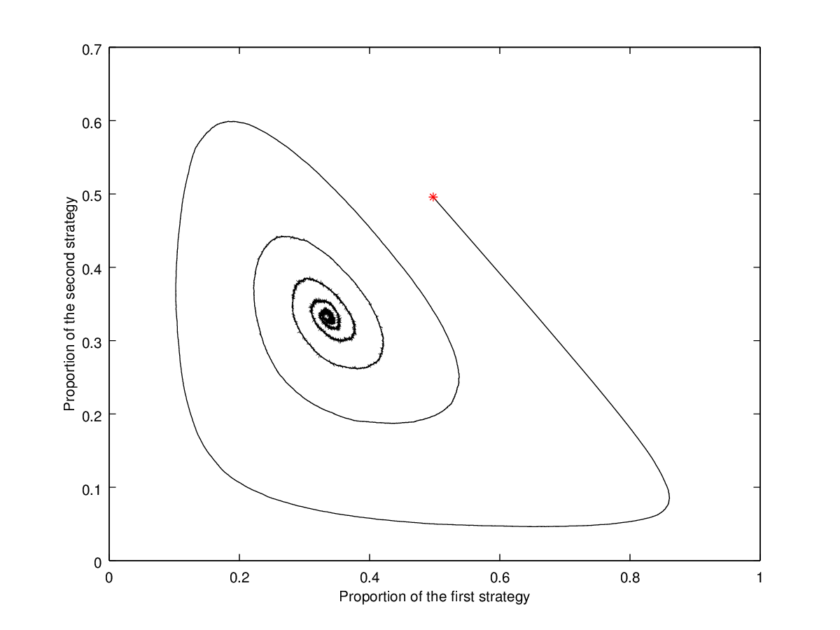
Figure 1. Evolution of $(\bar{p}_{1},\bar{p}_{2})$ for the rock-paper-scissors game. Initially, $10^{4}$ players started near $(1/2,1/2,0)$. In the simulation they performed $4\times 10^{6}$ random matches with $\delta=0.05$.

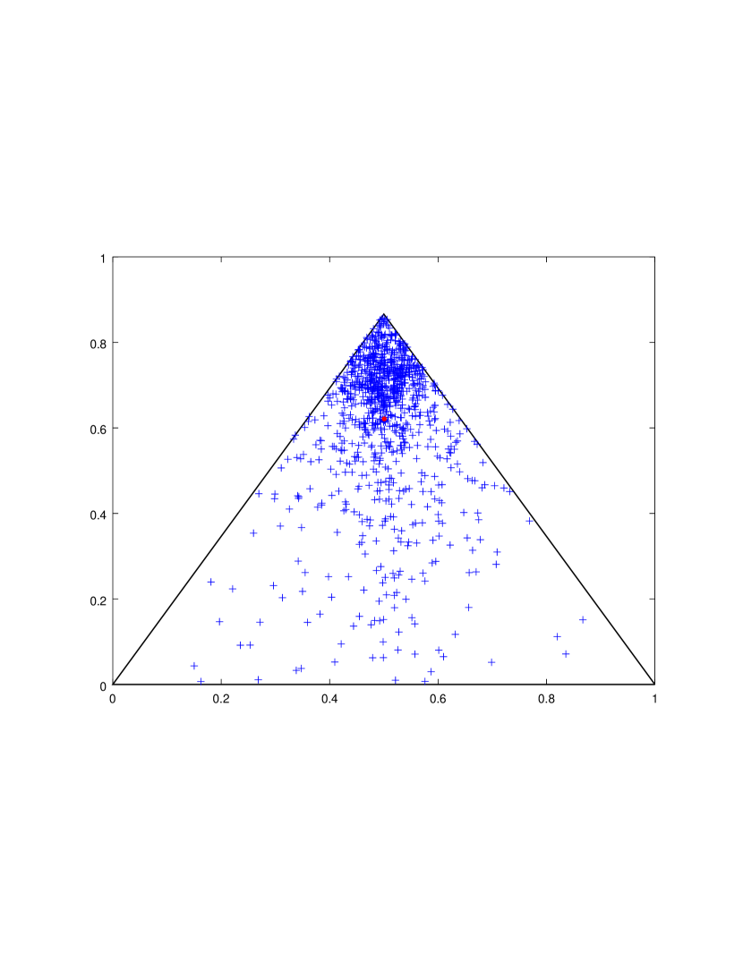
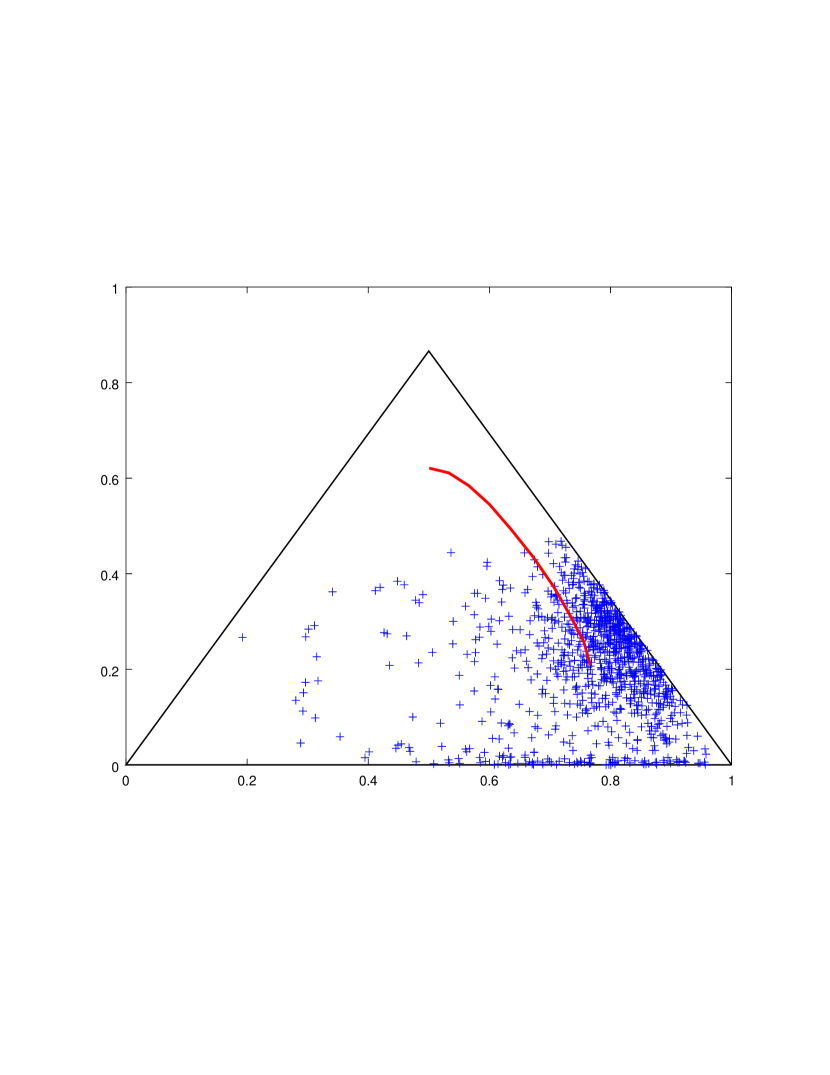
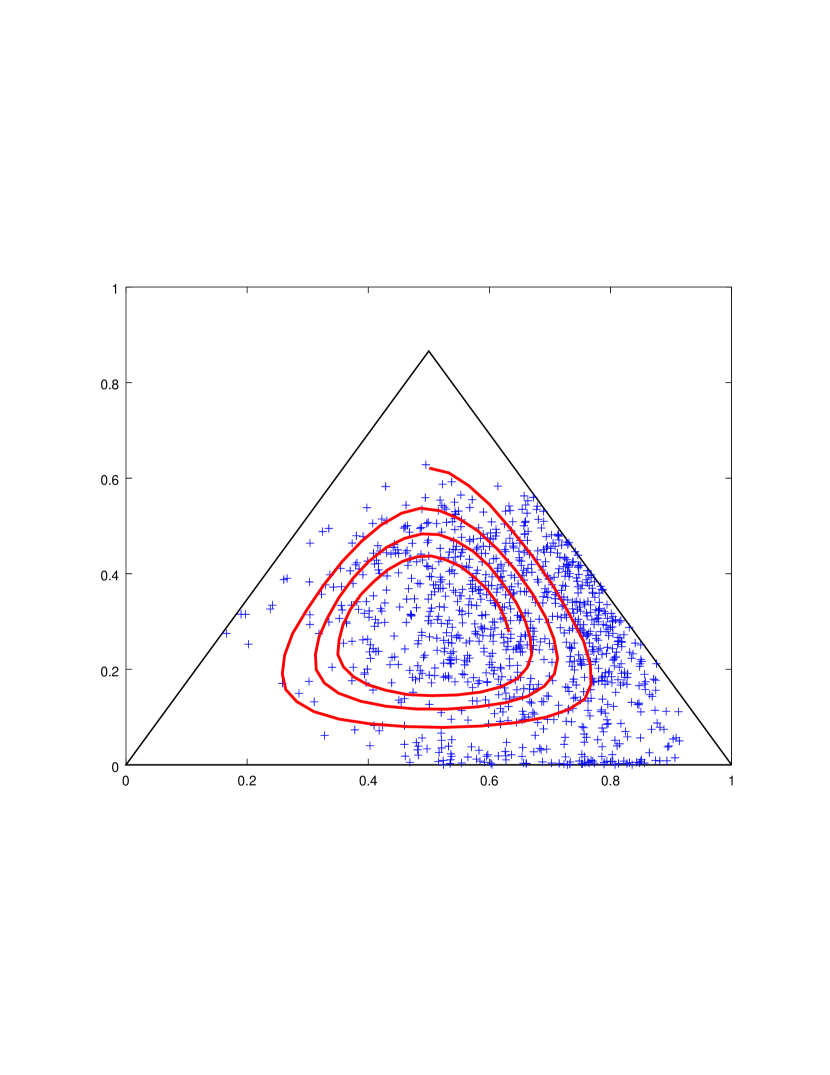
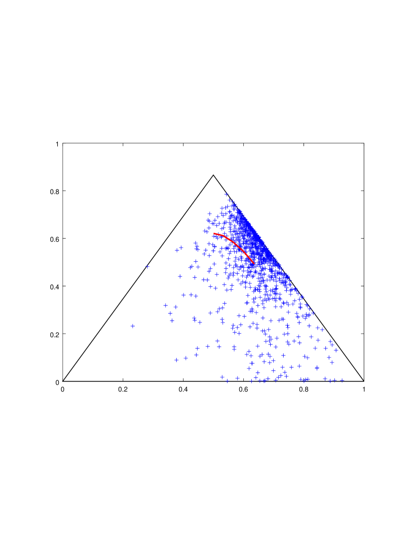
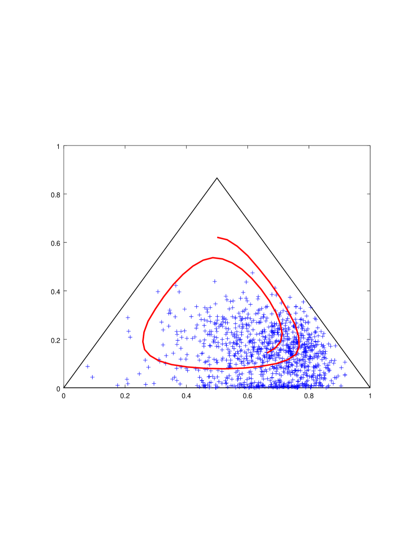
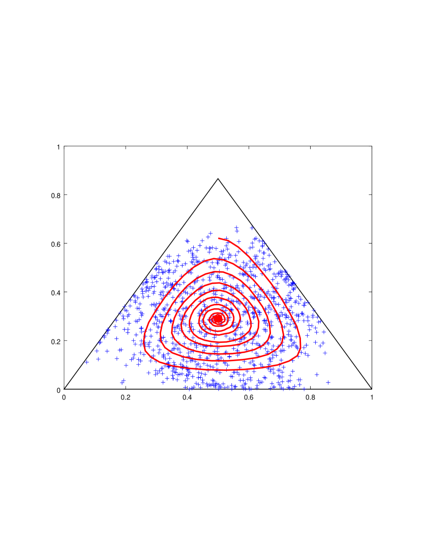
Figure 2. Diffusion of the players on the simplex of strategies. The first image is the initial distribution of the players, and the next ones are snapshots at steps 5, 10, 45, 100, and 1000. In each step, every agent is sequentially selected and randomly matched with another player.The solid line correspond to the trajectory of the mean strategy of the population.

5. Wealth distribution among the agents

In this section we present the effect of the games on the wealth distribution curves. We start with two strategies games and then we consider the rock-paper-scissors game. Let us observe that in the former case, the players learn how to play the optimal pure strategy, and then the wealth distribution frozen since the payoff at equilibrium is zero; we are interested here in the initial advantage of a player who is close to the optimal strategy. In the latter case, the agents play a mixed strategy, and we compute the expected value of the variance due to the fluctuations of agents wealth; we find a remarkable agreement with the simulations.

Let us introduce the family of probability densities $\{P_{t}(w)\}_{t\geq 0}$, and the probability to find an agent whose wealth belong to some interval $(a,b)$ at time $t$ is given by

$$\int_{a}^{b}P_{t}(w)dw.$$

Now we compute the variance of $P_{t}(w)$ in order to compare it with our simulations. We have the following result:

Theorem 5.1.

Let $G$ be the matrix of a symmetric zero sum game, and let us consider the wealth evolution process generated by the microscopic interaction rule (1). Let us assume that the players are playing a mixed Nash equilibrium $p$, and that they are selected at random from the distribution $P_{t}$. Then, for sufficiently small $\varepsilon$, we have

$$\lim_{t\to\infty}\mathbb{E}(w^{2})=\frac{\langle G^{+}\rangle}{-\varepsilon\langle G^{+2}\rangle+\langle G^{+}\rangle},$$

where

$$\langle G^{\pm}\rangle =\varepsilon^{-1}\iint pG_{\varepsilon}^{\pm}p^{\prime}\,P_{t}(w)P_{t}(w^{\prime})dwdw^{\prime}$$

$$\langle G^{\pm 2}\rangle =\varepsilon^{-2}\iint(pG_{\varepsilon}^{\pm}p^{\prime})^{2}\,P_{t}(w)P_{t}(w^{\prime})dwdw^{\prime},$$

Proof.

Using the interaction rule, and the distribution of players we have

$$\frac{d}{dt}\mathbb{E}(w^{2})= \frac{d}{dt}\int w^{2}P_{t}(w)dw$$

$$= \iint\big{[}(w+pG_{\varepsilon}^{+}p^{\prime}w^{\prime}-pG_{\varepsilon}^{-}p^{\prime}w)^{2}-w^{2}\big{]}P_{t}(w)P_{t}(w^{\prime})dwdw^{\prime}$$

$$= \iint\big{[}(pG_{\varepsilon}^{+}p^{\prime})^{2}(w^{\prime})^{2}+2ww^{\prime}(pG_{\varepsilon}^{+}p^{\prime})\big{]}P_{t}(w)P_{t}(w^{\prime})dwdw^{\prime}$$

$$+\iint\big{[}(pG_{\varepsilon}^{-}p^{\prime})^{2}-2(pG_{\varepsilon}^{-}p^{\prime})\big{]}(w)^{2}P_{t}(w)P_{t}(w^{\prime})dwdw^{\prime}$$

$$-\iint(pG_{\varepsilon}^{+}p^{\prime})(pG_{\varepsilon}^{-}p^{\prime})ww^{\prime}P_{t}(w)P_{t}(w^{\prime})dwdw^{\prime}.$$

We use now that $\mathbb{E}(w^{2})=\mathbb{E}(w^{{}^{\prime}2})$, $\mathbb{E}(w)=\mathbb{E}(w^{\prime})=1$ and that

$$\iint(pG_{\varepsilon}^{+}p^{\prime})(pG_{\varepsilon}^{-}p^{\prime})ww^{\prime}P_{t}(w)P_{t}(w^{\prime})dwdw^{\prime}=0,$$

since for each pure strategy, one of the two games is equal to zero. Therefore,

$$\frac{d}{dt}\mathbb{E}(w^{2})= \varepsilon^{2}\langle G^{+2}\rangle\mathbb{E}(w^{2})+2\varepsilon\langle G^{+}\rangle$$

$$+\varepsilon^{2}\langle G^{-2}\rangle\mathbb{E}(w^{2})-2\varepsilon\langle G^{-}\rangle\mathbb{E}(w^{2})$$

We observe that $u(t)=\mathbb{E}(w^{2})$ is a solution of the ordinary differential equation

$$\frac{d}{dt}u(t)=Au(t)+B,$$

for $A=\varepsilon^{2}\langle G^{+2}\rangle+\varepsilon^{2}\langle G^{-2}\rangle-2\varepsilon\langle G^{-}\rangle$, and $B=2\varepsilon\langle G^{+}\rangle$, with some initial condition $u_{0}=\mathbb{E}(w_{0}^{2})$ depending on the initial distribution of wealth. The explicit solution is

$$\mathbb{E}(w^{2})=C(A,u_{0})exp(At)-A^{-1}B,$$

and

$$\lim_{t\to\infty}\mathbb{E}(w^{2})=\frac{-2\langle G^{+}\rangle}{\varepsilon\langle G^{+2}\rangle+\varepsilon\langle G^{-2}\rangle-2\langle G^{-}\rangle}$$

since $A<0$ for $\varepsilon$ small enough.

The result follows since $\langle G^{+}\rangle=\langle G^{-}\rangle$ and $\langle G^{+2}\rangle=\langle G^{-2}\rangle$ due to the symmetry of the game, and the proof is finished. ∎

Let us remark that the previous proof holds in the limit of infinitely many players. Of course, if the number of players is finite, we can understand $P_{t}$ as a sum of Dirac’s delta functions.

5.1. Simulations for $2\times 2$ games

We have considered a symmetric game with two strategies $s_{1}$ and $s_{2}$, and the pay-off matrix $G$ has the form

$$G=\begin{pmatrix}0&\varepsilon\\ -\varepsilon&0\end{pmatrix}$$

for $\varepsilon\in(0,1)$.

As was proved in Subsection 4.1, we observe that all the players learn how to play the optimal strategy. As a consequence, the wealth distribution reaches an equilibrium which is highly dependent on the duration of the transient state while the agents learn the optimal way of play, and then is frozen. So, it is interesting to study the effect of the strategy update step $\delta$ on the steady state.

In the following figures we have run Algorithm 1 with $10^{4}$ agents, each agent with wealth $1$, and $\varepsilon=0.1$. We have fixed the vector of initial strategies for each player and we have performed 100 simulations starting with these initial strategies. In Figure 3 we observe the mean steady state curve for these simulations, for $\delta=0.1$ (left), $\delta=0.01$ (center), and $\delta=0.001$ (right).

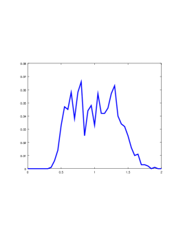
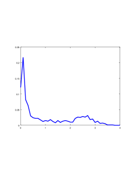
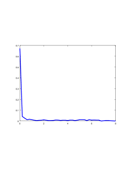
Figure 3. Steady state of the wealth for different values of $\delta$, $\delta=0.1$ (left), $\delta=0.01$ (center), and $\delta=0.001$ (right). We averaged 100 simulations with $N=10^{4}$ agents and the same initial distribution of strategies.

In Figure 4 we show the mean wealth obtained at the steady state for the agents as a function of their initial strategy. The horizontal axis represent the probability that an agent play the optimal strategy, and clearly the ones which started with a high probability to play it become more wealthier. Here, the value of $\delta$ determines the duration of the transient state, where the wealth exchange takes place. We have $\delta=0.1$ (left), $\delta=0.01$ (center), and $\delta=0.001$ (right).

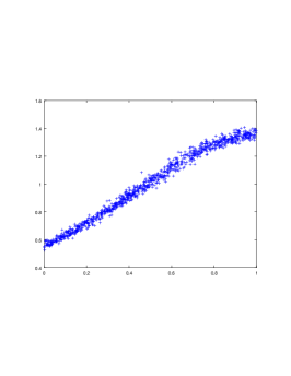
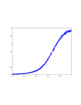
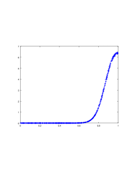
Figure 4. Mean wealth of agents (vertical axis) depending on their initial probability to play the optimal strategy (horizontal axis), for different values of $\delta$, $\delta=0.1$ (left), $\delta=0.01$ (center), and $\delta=0.001$ (right). We averaged 100 simulations with $N=10^{4}$ agents and the same initial distribution of strategies.

5.2. The Rock-paper-scissors game

Let us consider now the Rock-paper-scissors game from Subsection 4.1.2. We fix $a=b=1$, and we scale the game with different parameters $\varepsilon\in(0,1)$.

In Figure 5 we show several histograms, for different values of $\varepsilon$, of the wealth distribution for $N=10^{4}$ agents, averaged over $10$ realizations starting all of them with the same initial strategies, and each agent has initial wealth equal to $1$. Let us note that we have less equalitarian distributions when $\varepsilon$ approaches $1$. In fact, for $\varepsilon=1$, all the wealth is transferred to the winner player, and in the long run, it accumulates in a single player.

The solid lines in Figure 5 represent the Gamma function

$$\Gamma(x)=\frac{v^{v}\exp(-vx)}{\Gamma(v)x^{1-v}},$$

where $v=v(\varepsilon)$ is the sample variance of the data in each case. We show in Table 1 that the sample variance and the theoretical value $\varepsilon(1-\varepsilon)^{-1}$ are very close.

The value $v(\varepsilon)=\varepsilon(1-\varepsilon)^{-1}$ can be computed from Theorem 5.1, or using directly the interaction rule, from

$$w_{i}^{*}=w_{i}+\varepsilon(g_{lm}^{+}w_{j}-g_{lm}^{-}w_{i}).$$

Let us note that the expected value of $w_{i}$ is $\mathbb{E}(w_{i})=1$, hence the variance is

$$Var(w_{i})=\mathbb{E}(w_{i}^{2})-1.$$

Let us call $V=\mathbb{E}(w_{i}^{2})$. The linearity of the expected value, and the independence implies

$$\mathbb{E}([w_{i}^{*}]^{2})= \mathbb{E}([w_{i}+\varepsilon g_{lm}^{+}w_{j}-\varepsilon g_{lm}^{-}w_{i}]^{2})$$

$$= \mathbb{E}([w_{i}]^{2})+\mathbb{E}([\varepsilon g_{lm}^{+}w_{j}]^{2})+\mathbb{E}([\varepsilon g_{lm}^{-}w_{i}]^{2})+2\mathbb{E}(\varepsilon g_{lm}^{+}w_{j}w_{i})$$

$$\quad-2\mathbb{E}(\varepsilon g_{lm}^{-}w_{i}^{2})-2\mathbb{E}(\varepsilon^{2}g_{lm}^{+}g_{lm}^{-}w_{j}w_{i}).$$

Therefore,

$$V=V+\varepsilon^{2}\mathbb{E}([g_{lm}^{+}]^{2})V+\varepsilon^{2}\mathbb{E}([g_{lm}^{-}]^{2})V+\varepsilon 2\mathbb{E}(g_{lm}^{+})-2\varepsilon\mathbb{E}(g_{lm}^{-})V-\varepsilon^{2}2\mathbb{E}(g_{lm}^{+}g_{lm}^{-}),$$

which gives

$$V=\frac{2\mathbb{E}(g_{lm}^{+})-\varepsilon 2\mathbb{E}(g_{lm}^{+}g_{lm}^{-})}{2\mathbb{E}(g_{lm}^{-})-\varepsilon\mathbb{E}([g_{lm}^{+}]^{2})-\varepsilon\mathbb{E}([g_{lm}^{-}]^{2})}$$

Using that

$$\mathbb{E}(g_{lm}^{+})=\mathbb{E}(g_{lm}^{-})=\mathbb{E}([g_{lm}^{-}]^{2})=\mathbb{E}([g_{lm}^{+}]^{2})=\frac{1}{3},$$

and $\mathbb{E}(g_{lm}^{+}g_{lm}^{-})=0$ since one of them must be zero, we get

$$V=\frac{\frac{2}{3}}{\frac{2}{3}-\frac{2\varepsilon}{3}}=\frac{1}{1-\varepsilon}$$

and thus

$$Var(w_{i})=\frac{\varepsilon}{1-\varepsilon},$$

as stated before.

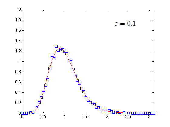
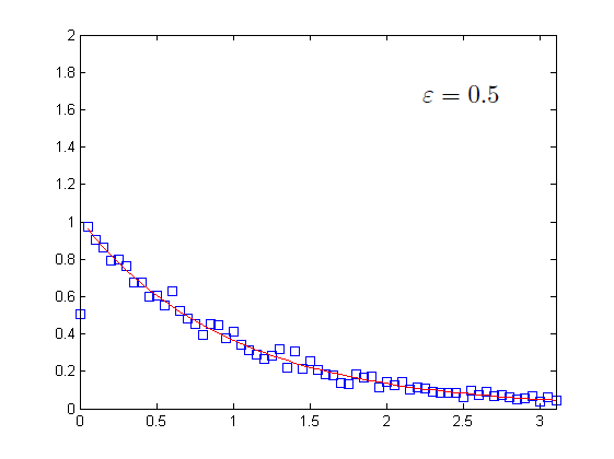
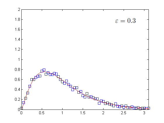
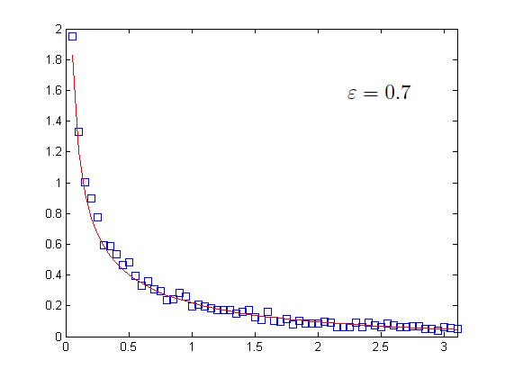
Figure 5. Histogram of the wealth distribution with $N=10^{4}$ agents, averaged over $10$ realizations, starting each one with wealth equal to $1$. The solid line represent the Gamma function of parameter $v=v(\varepsilon)$.

Value of $\varepsilon$	Sample variance	Theoretical value	Relative error
0.1	0.1114	0.1111	0.0030
0.3	0.4365	0.4286	0.0185
0.5	1.0098	1.0000	0.0098
0.7	2.3635	2.3333	0.0129
0.9	9.0967	9.0000	0.0107

Table 1. Variance of Gamma distribution depending of the value of $\varepsilon$.

6. Conclusions

In this work we have studied the wealth distribution problem when the agents interact through a zero sum game, which determine the wealth transfer. Moreover, we have studied the evolutive process, for agents using mixed strategies.

We have proposed a Pavlovian type of agents, which update their strategies myopically as a result of the last game they played, without trying to find the best response, or changing strategies proportionally to looses and gains, but reinforcing the winning strategy and penalizing the loosing strategy. A theoretical analysis of this simple dynamic gives a system of ordinary differential equations for the evolution of each agent strategies, and the mean strategy of the population solves a system very close to the replicator equation.

The wealth evolution of the population is similar to the one observed in more simple models where the interaction between agents is restricted to a random exchange of wealth. By scaling the game payoff we reproduce the saving propensity phenomena, and different Gamma-like curves appears as the steady state as a function of the scaling parameter.

Two different scenarios appear depending on the Nash equilibrium of the game. Since the game is symmetric, its value is zero, and when the Nash equilibrium is a pure strategy, the wealth transfer stops whenever the agents learn how to play in the optimal way. In this case we have more equalitarian distribution of wealth when they quickly update their strategies, and less equalitarian distribution when the evolutionary process is slow.

However, when the Nash equilibrium is a mixed strategy, the wealth transfer continues due to the random results of each individual game, and the steady state for the wealth distribution resembles the curves obtained using purely random ways to determine the wealth transfer. The shape of the steady state varies with the proportion of the agent’s wealth that is involved in each transaction, and more equalitarian distributions are obtained when this proportion is small, and if we allow to exchange almost all the wealth in a single game, we get a distribution strongly concentrated near zero, since wealth is accumulated in few individuals.

Finally, two directions seem promising. In the limit of infinitely many players we can expect a system of two coupled Boltzmann equations, one describing the evolutionary process on the simplex of strategies, and the other one modeling the wealth exchange.

On the other hand, new situations can occur whenever the agents play an arbitrary game. Beside the dichotomy between pure and mixed equilibria, we can have more than one equilibria, with different payoffs, and different kind of wealth distribution can appear depending on the limit equilibria selected by the dynamics. Let us remak that in this case the wealth is not conserved, and some kind of rescaling will be needed in order to study the asymptotic behavior of the wealth distribution.

Juan Pablo Pinasco Departamento de Matemática, FCEyN - Universidad de Buenos Aires and IMAS, CONICET-UBA Ciudad Universitaria, Pabellón I (1428) Av. Cantilo s/n. Buenos Aires, Argentina. e-mail:jpinasco@dm.uba.ar

Mauro Rodriguez Cartabia Departamento de Matemática, FCEyN - Universidad de Buenos Aires and IMAS, CONICET-UBA Ciudad Universitaria, Pabellón I (1428) Av. Cantilo s/n. Buenos Aires, Argentina. e-mail:mrodriguezcartabia@gmail.com

Nicolas Saintier Departamento de Matemática, FCEyN - Universidad de Buenos Aires and IMAS, CONICET-UBA Ciudad Universitaria, Pabellón I (1428) Av. Cantilo s/n. Buenos Aires, Argentina. e-mail:nsaintie@dm.uba.ar

References

- [1] O. Bournez, J. Chalopin, J. Cohen, X. Koegler, M. Rabie. Computing with pavlovian populations. In International Conference On Principles Of Distributed Systems, pp. 409-420. Springer Berlin Heidelberg, 2011.
- [2] B. K. Chakrabarti, A. Chakraborti, S. R. Chakravarty, A. Chatterjee, Econophysics of income and wealth distributions, Cambridge University Press, 2013.
- [3] A. Chatterjee, B. K. Chakrabarti, S. S. Manna. Pareto law in a kinetic model of market with random saving propensity. Physica A: Statistical Mechanics and its Applications 335 (2004) 155-163.
- [4] D. Friedman, On economic applications of evolutionary game theory. J. Evol. Econ. 8 (1998) 15-43.
- [5] A. K. Gupta, Money exchange model and a general outlook. Physica A: Statistical Mechanics and its Applications 359 (2006) 634-640.
- [6] J. Hofbauer, P. Schuster, K. Sigmund. A note on evolutionarily stable strategies and game dynamics. J Theor Biol. 81 (1979) 609-612.
- [7] J. Hofbauer, K. Sigmund, Evolutionary games and population dynamics. Cambridge University Press (1998).
- [8] D. Kraines, V. Kraines. Pavlov and the prisoner’s dilemma. Theory and Decision 26 (1989) 47-79.
- [9] J.W. Eaton. GNU Octave, https://www.gnu.org/software/octave/
- [10] R. Cressman, Y. Tao. The replicator equation and other game dynamics. Proc Natl Acad Sci U S A 111 (2014) 10810-10817.
- [11] L. Pareschi, G. Toscani. Self-similarity and power-like tails in nonconservative kinetic models. Journal of Statistical Physics 124 (2006) 747-779.
- [12] V. Pareto, Cours d’economie politique. Rouge, Lausanne, 1897.
- [13] M. Patriarca, A. Chakraborti, G. Germano. Influence of saving propensity on the power law tail of wealth distribution. Physica A: Statistical Mechanics and its Applications 369 (2) 723-736.
- [14] M. Patriarca A. Chakraborti, K. Kaski, Statistical model with a standard distribution. Physical Review E 70 (2004) 016104.
- [15] P. Repetowicz, S. Hutzler, P. Richmond. Dynamics of money and income distributions. Physica A: Statistical Mechanics and its Applications 356 (2005) 641-654.
- [16] W. H. Sandholm, Population games and evolutionary dynamics, MIT Press, 2010.
- [17] C. Silva, W. Pereira, J. Knotek, P. Campos. Evolutionary Dynamics of the Spatial Prisoner’s Dilemma with Single and Multi-Behaviors: A Multi-Agent Application. Chapter 49 in Dynamics, Games and Science II DYNA 2008, in Honor of Mauricio Peixoto and David Rand, editors M. Matos Peixoto, A. Adrego Pinto, D. A. Rand, Springer, 2011.
- [18] M. N. Szilagyi. A general N-person game solver for pavlovian agents. Complex Systems 24 (2015) 261-274.
- [19] P. D. Taylor, L. Jonker. Evolutionary stable strategies and game dynamics. Math Biosci. 40 (1978) 145-156.
- [20] E. C. Zeeman. Population dynamics from game theory. In Proceedings of an international conference on global theory of dynamical systems, editors A. Nitecki, C. Robinson. Berlin: Springer; 1980. Lecture Notes in Mathematics 819.