Low-memory GEMM-based convolution algorithms for deep neural networks

Abstract

Deep neural networks (DNNs) require very large amounts of computation both for training and for inference when deployed in the field. A common approach to implementing DNNs is to recast the most computationally expensive operations as general matrix multiplication (GEMM). However, as we demonstrate in this paper, there are a great many different ways to express DNN convolution operations using GEMM. Although different approaches all perform the same number of operations, the size of temorary data structures differs significantly. Convolution of an input matrix with dimensions $C\times H\times W$, requires $O(K^{2}CHW)$ additional space using the classical im2col approach. More recently memory-efficient approaches requiring just $O(KCHW)$ auxiliary space have been proposed.

We present two novel GEMM-based algorithms that require just $O(MHW)$ and $O(KW)$ additional space respectively, where $M$ is the number of channels in the result of the convolution. These algorithms dramatically reduce the space overhead of DNN convolution, making it much more suitable for memory-limited embedded systems. Experimental evaluation shows that our low-memory algorithms are just as fast as the best patch-building approaches despite requiring just a fraction of the amount of additional memory. Our low-memory algorithms have excellent data locality which gives them a further edge over patch-building algorithms when multiple cores are used. As a result, our low memory algorithms often outperform the best patch-building algorithms using multiple threads.

I Motivation

Deep neural networks are among the most successful techniques for processing image, video, sound and other data arising from real-world sensors. DNNs require very large amounts of computation which challenge the resource of all but the most powerful machines. However, DNNs are also most useful when deployed in embedded devices that interact directly with the surrounding world. Thus there is a tension between the resources needed by deep neural networks, and the kind of embedded devices that can make best use of deep learning technology by applying it to live data from embedded sensors.

DNNs consist of an acyclic directed graph of “layers” that receive raw input data, and commonly output a classification of the data. Data flows along edges between layers. Each layer processes its input data, and produces output data on its outgoing edges. Several different types of layers are used to implement DNNs, such as activation layers, pooling layers, convolution layers, and fully-connected layers. In the best-known DNNs a great majority of the execution time is spent in the convolution layers.

There are many ways that each layer can be implemented. For example, early DNN libraries simply implemented each layer with a loop nest. However, Yangqing Jia discovered that the convolution layers could be implemented more efficiently by restructuring the data and calling a standard matrix multiplication routine. Most machines already have a fast implementation of the Basic Linear Algebra Subprograms (BLAS), which includes a general matrix multiplication (GEMM) routine. BLAS libraries are carefully hand-coded, and may include code generation and auto-tuning systems to maximize performance. Implementing convolution using GEMM allows the developer to exploit these highly-tuned routines.

DNN layers can be implemented in other ways. For example, many layers are implemented as carefully coded loop nests that provide a direct implementation of the layer [1]. Another common approach is to convert the data to another format, such as the Fourier domain, where convolution can be computed efficiently [2]. Several authors have also proposed domain-specific code generators, that can generate many variants of the code for a problem and use auto-tuning to select a fast version [3].

We study a variety of different approaches to implementing DNN convolution using the BLAS GEMM routine. By rewriting the convolution as different variants of GEMM calls with different data layouts, we can trade off execution time, memory requirements and parallelism within a framework that is suitable for automation. Our main contributions are as follows:

• We provide the first systematic study of the design space of DNN convolution implementation using GEMM.

• We note that the most popular existing patch-building DNN convolution algorithms require $O(CHWK^{2})$ additional temporary space. Even the most memory-efficient GEMM-based DNN convolution algoirithm needed $O(CHWK)$ additional space.

• We propose two novel GEMM-based algorithms for DNN convolution based on accumulating the results of smaller convolutions. The two algorithms require only $O(MHW)$ and $O(KW)$ additional space respectively.

• We evaluate a very large range of GEMM-based convolution algorithms and variants on Intel Core i7 and ARM Cortex A57 processors. We find that our low-memory DNN convolution algorithms can be just as fast as the best patch-building algorithms despite needing only a fraction of the space.

• In addition we find that when multiple cores are used to perform the convolution, the low memory requirements of our algorithms improves locality to the point that they are often faster than equivalent patch-building algorithms.

II DNN convolution

DNNs consist of a directed graph of standard layers which operate on data on incoming edges and place results on outgoing edges. In many DNNs, the majority of execution time is occupied by convolution layers. A convolutional layer takes operates on two source tensors and produces another tensor as output. In C code, these tensors might be repesented as:

float input[C][H][W];
float kernels[M][C][K][K];
float output[M][H][W];

A convolution layer consists of four components: 1) a 3D tensor $\mathcal{I}\in\mathbb{R}^{H\times W\times C}$ which acts as as the input to the convolution layer 2) a set of “kernels” or “filters” represented by a 4D tensor $\mathcal{K}\in\mathbb{R}^{M\times C\times K\times K}$ 3) a bias term per filter 4) and a 3D output tensor. Multiple Channel Multiple Kernel (MCMK) is typically constructed as the concatenation of the output of $M$ Multiple Channel Single Kernel (MCSK) as described by Vasudevan et al. [4] is often represented as nested summations as,

ΨΨΨinput[C][H][W];
ΨΨΨkernels[M][K][K][C];
ΨΨΨoutput[M][H][W];
ΨΨΨfor h in 1 to H do
ΨΨΨ  for w in 1 to W do
ΨΨΨ    for o in 1 to M do
ΨΨΨ      sum = 0;
ΨΨΨ      for x in 1 to K do
ΨΨΨ        for y in 1 to K do
ΨΨΨ          for i in 1 to C do
ΨΨΨ            sum += input[i][h+y][w+x]
ΨΨΨ                   *kernels[o][x][y][i];
ΨΨΨ      output[o][w][h] = sum;
ΨΨΨ

Figure 1: Simplified code for 2D multi-channel convolution with a single multi-channel input and multiple multi-channel convolution kernels. Note that special treatment of edge boundaries is not shown in this code.

III Convolution with $O(K^{2}CHW)$ patch matrix

An attractive approach to implementing DNN convolution is to recast it as matrix multiplication and use highly optimized routines such as general matrix multiplication (GEMM) to find the solution. The $im2col$ approach [5, 6, 7, 8] has been well studied for transforming the Multiple Channel Multiple Kernel (MCMK) problem into a General Matrix Multiplication (GEMM) problem. Consider an input $\mathcal{I}\in\mathbb{R}^{H\times W\times C}$ and $M$ kernels $\mathcal{K}\in\mathbb{R}^{M\times K\times K\times C}$. From the input $\mathcal{I}$ we construct a new input-patch-matrix $\hat{\mathcal{I}}$, by copying patches out of the input and unrolling them into columns of this intermediate matrix. These patches are formed in the shape of the kernel (i.e. $K\times K\times C$) at every location in the input where the kernel is to be applied.

Once the input-patch-matrix $\hat{\mathcal{I}}$ is formed, we construct the kernel-patch-matrix $\hat{\mathcal{K}}$ by unrolling each of the $M$ kernels of the shape $K\times K\times C$ into a row of $\hat{\mathcal{K}}$. Note that this step can be avoided if the kernels are stored in this format to begin with (innermost dimension is the channel which forces the values along a channel to be contiguous). Then we simply perform a GEMM of $\hat{\mathcal{K}}$ and $\hat{\mathcal{I}}$ to get the output $\hat{\mathcal{O}}\in\mathbb{R}^{H\times W\times M}$ as shown in the figure.

III-A Matrix layouts

The inputs and outputs of convolution are multidimensional tensors, so there are a great many possible orderings of the dimensions. Many DNN implementations use a single canonical tensor layout. For example, Caffe [9] lays out the dimensions of input data tensors in the order $C\times H\times W$ (or more briefly $CHW$), and builds patch matrices with dimensions $CKKHW$. When invoking the GEMM operation the patch matrix is interpreted as a 2D matrix of dimensions $CKK\times HW$.

Building the patch matrix is a simple operation. But any dimension ordering might be used for the input or patch matrix, so there are many variants. One possible method for implementing $im2col$ is by creation of patches that each occupy a column of the patch matrix. It is easy to imagine another variant where each patch instead occupies a row of the resulting matrix. Vasudevan et al. [4] refer to this variant as im2row ($im2row$).

An additional complication when describing these variants is that there are two competing layouts of rows and columns in memory. Fortran uses a column-major format, where matrix elements that are adjacent in memory are interpreted as being in the same row of the matrix. C/C++ use row-major format, where elements from the same row are adjacent in memory. GEMM is originally a Fortran routine, and therefore assumes a column-oriented layout, but many DNN implementations are in C/C++, which may result in confusion about array formats in memory. For this reason we often refer to patch matrices as being patch-major or KKC-major meaning that elements of the same patch are adjacent in memory. Another possible layout is HW-major or patch-minor, where elements of the non-patch dimension of the patch matrix are adjacent in memory.

float input[H][W][C];
float patches[H][W][K][K][C];
for ( h = 0; h < H; h++ )
  for ( w = 0; w < W; w++ )
    for ( kh = -K/2; kh < K/2; kh++ )
      for ( kw = -K/2; kw < K/2; kw++ )
        for ( c = 0; c < C; c++ )
          patches[h][w][kh][kw][c]
                 = input[h+kh][w+kw][c];

Figure 2: Building the $KKC$-major patch matrix

Figure 2 shows a loop nest for constructing a patch matrix from the input. The patch matrix has dimentions HWKKC, which allows us to consider as a five dimensional $H\times W\times\times K\times K\times C$ matrix, or a two-dimensional $HW\times KKC$ matrix. The C/C++ code in Figure 2 assumes a row-major layout, which implies a patch-major or KKC-major format.

A key step of building the patch matrix is gathering elements of the input matrix. As shown in Figure 2, the major dimension of input is the $C$ dimension. The loop nest in Figure 2 copies items from the input to the patch matrix. The innermost loop copies adjacent elements of C-major input matrix to adjacent elements of the patch matrix. The result is that the code in Figure 2 has extremely good spatial locality, and is therefore very fast in practice.

III-B Patch-minor layouts

Other layouts can result in very different data locality. For example, consider the case where the patch matrix is HW-major rather than patch-major. Figure 3b shows an example of such a matrix where, for simplicity we have assumed $C=1$. If we were to construct the shaded patch column of Figure 3b by gathering the corresponding shaded patch elements of Figure 3a in sequence, the spatial locality would be extremely poor.

However, an alternative strategy results in much better spatial locality. Note that the each row of the patch matrix contains a row of the input. Therefore, if the input format is compatible, even a non-patch-major patch matrix can be constructed with excellent spatial locality. Furthermore, even if the input does is not suitable for directly copying rows to the patch matrix, it is nonetheless possible to achieve almost as good spatial locality. Note the successive rows of Figure 3b contain repeated sequences of data. Once the first row containing that data has been gathered, it is therefore possible to simply copy data from one row of the patch matrix to the next.

This strategy of copying sequences of data from one row of a patch matrix to the next is particularly important for strided DNN convolution. A patch matrix for a convolution with stride $S$ has only $HW/S$ patches as shown in Figure 3c. Thus, the sequences of values across the rows of a column-oriented patch matrix do not match the original matrix layout. However, once the first row containing a particular set of data has been collected, the data can be copied to later rows containing the same sequence of values. To our knowledge we are the first to exploit spatial locality between rows in this way, when computing column-oriented patch matrices in row-major matrix layouts.

a0	a1	a2	a3	a4
b0	b1	b2	b3	b4
c0	c1	c2	c3	c4
d0	d1	d2	d3	d4

(a) Input matrix

0	0	a0	a1	a2	a3	a4
0	a0	a1	a2	a3	04	0
a0	a1	a2	a3	a4	0	0
0	0	b0	b1	b2	b3	b4
0	b0	b1	b2	b3	b4	0
b0	b1	b2	b3	b4	0	0
0	0	c0	c1	c2	c3	c4
0	c0	c1	c2	c3	c4	0
c0	c1	c2	c3	c4	0	0

(b) Patch matrix of $3\times 3$ patches

0	a0	a2	a4
0	a1	a3	0
a0	a2	a4	0
0	b0	b2	b4
0	b1	b3	0
b0	b2	b4	0
0	c0	c2	c4
0	c1	c3	0
c0	c2	c4	0

(c) Stride 2 patch matrix

Figure 3: Sub-parts of input matrix and column patch matrix, and strided patch matrix with patches of size $3\times 3$. The shaded part is a corresponding patch in each matrix. The outermost dimension, $C$, is not shown.

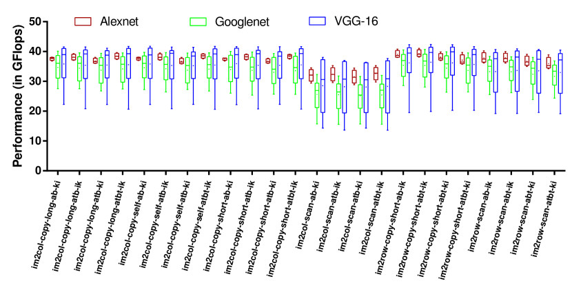
Figure 4: Performance of GEMM-based convolution with $O(K^{2}CHW)$ patch matrix

III-C Patch-building Algoritms

($im2col-scan$): The $im2col-scan$ method uses a patch building procedure that is very similar to the method outlined in 2 where each $KKC$ column of the patch matrix is built sequentially. While this method is simple to understand and can produce strided and unstrided patch matrix it has very poor spatial locality while accessing the input as each column of the patch matrix will use values from a number of the input’s rows and columns.

($im2col-copy-self$): The $im2col-copy-self$ method is an improvement on the $im2col-scan$ method. From 3b we can see that many of the rows share large contiguous sections of the same values. With this we only need to use $im2col-scan$ to build a minority of the rows and then can use memory copying functions to construct the other rows of the patch matrix much faster.

($im2col-copy-long$): Looking at 3b we can see that the rows of the patch matrix are built from contiguous sections of the input (given a row-major input). With this we can build the patch matrix more quickly by copying entire sections of the input into the patch matrix. Note however that this property does not hold with 3c so this method can not be used for strided patch matrix.

($im2col-copy-short$): $im2col-copy-short$ is very similar to $im2col-copy-long$. The difference comes in the fact that while not shown in 3b some of the values in the large contiguous sections copied from the input to the patch matrix will be replaced by zeroes. In $im2col-copy-long$ we copy the longest possible section and then go back replacing values with zeroes where needed. In $im2col-copy-short$ we copy the values up to each zero, insert the zero, then copy the next section. Also note ($im2row-copy-short$) does not exist but, ($im2row-copy-short$) can create strided patch matrix unlike $im2col-copy-short$.

III-D Evaluation

Figure 4 exhibits the trade-offs between the different data layouts and the patch building algorithms discussed in section III-C. The suffixes -ab-ki denote the type of GEMM used. For instance, the first part of suffix denotes the layout of the two matrices. ab is the default GEMM, while atb, abt and atbt correspond to the respective GEMM call. The second part of the suffix denotes the order of the multiplication. ik performs input times kernel while ki performs kernel times input. These suffix notations are used throughout the rest of the paper and hold the same meaning.

The results for AlexNet, GoogLeNet and VGG-16 are shown on the same graph as box and whiskers. This type of graph gives a lot of information about what are the operating characteristics of the methods in each network. The minimum and maximum performance delivered by the methods are shown by the whiskers, while the box shows the 5 and 95 percentiles while the dash in the middle of the box shows the 50^th percentile. The average performance of the method is indicated by the small + inside the box.

It is fairly evident from the scales of the box and whiskers from the graph that most of the im2 methods deliver performance in a small band. This implies that the performance delivered by a method is similar for all the layers in alexnet thereby making the variance in performance low. On the other hand, the variance increases in GoogLeNet and is the highest in VGG-16. Another observation is that all the $im2col-scan$ variants produce significantly lower performance compared to the rest of the im2 methods. This is in keeping with our intuition as the $im2col-scan$ patch building algorithm has the worst locality amongst all the patch building methods.

IV Convolution with $O(K^{2}MHW)$ result matrix

A major problem with the convolution methods from Section III is that the patch matrix requires $K^{2}$ more memory than the original image, which is a dramatic increase in the size of the input. This additional space may reduce data locality, increase memory traffic, and may exceed the available memory in embedded systems.

Figure 1 shows a simplified loop nest for $K\times K$ convolution with $M$ kernels each with $C$ channels. A common operation in Convolutional Neural Networks (CNNs) such a GoogLeNet [10] is convolution with a set of $1\times 1$ convolutions. If we consider the code in figure 1 for the case where $K=1$, then the $x$ and $y$ loops collapse into a single iteration.

The resulting code is equivalent to 2D matrix multiplication of a $M\times C$ kernel times a $[C]\times[H\times W]$ input which results in a $[M]\times[H\times W]$ output. This output however is actually $M$ planes of $H\times W$ pixels which corresponds to an output of size $[H]\times[W]$ and $M$ channels. Let us call this correspondence of a $[M]\times[H\times W]$ matrix to an output matrix of size $[H]\times[W]$ and $M$ channels its multi-channel representation, which we will use throughout the rest of this section. In other words, $1\times 1$ MCMK can be implemented by simply calling GEMM without data replication.

IV-A $kn2row$ and Kernel to Column ($kn2col$)

Given that we can compute $1\times 1$ MCMK without data replication, how can we implement $K\times K$ MCMK, for $K>1$? We argue that a $K\times K$ convolution can be expressed as the sum of $K^{2}$ separate $1\times 1$ convolutions. However the sum is not trivial to compute. Each $1\times 1$ convolution yields a result matrix with dimensions $[M]\times[H\times W]$. We cannot simply add each of the resulting matrices pointwise, as each resultant matrix corresponds to a different kernel value in the $K\times K$ kernel. The addition of these matrices can then be resolved by offsetting every pixel in every channel of the multi-channel representation of these matrices, vertically and/or horizontally (row and column offsets) by one or more positions before the addition.

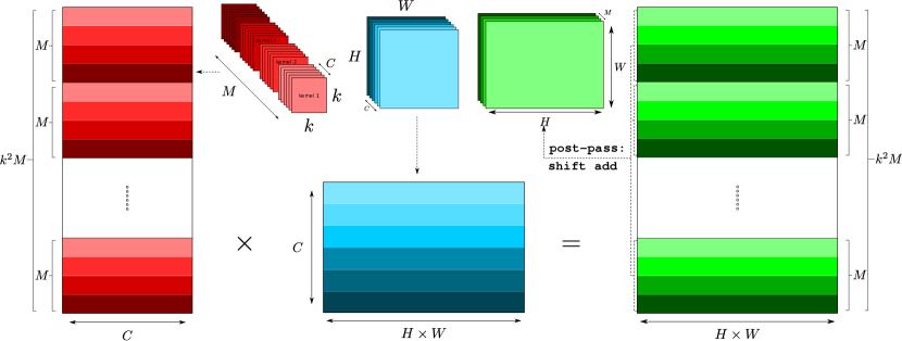
Figure 5: MCMK using the “$kn2row$” method

For example, when computing a $3\times 3$ convolution the result from computing the $1\times 1$ MCMK for the central point of the $3\times 3$ kernel is perfectly aligned with the final sum matrix. On the other hand, the matrix that results from computing the $1\times 1$ MCMK for the upper left value of the $3\times 3$ kernel must be offset up by one place and left by one place (in its multi-channel representation) before being added to the final sum that computes the $3\times 3$ MCMK. Note that when intermediate results of $1\times 1$ convolutions are offset, some values of the offsetted matrix fall outside the boundaries of the final result matrix. These out-of-bounds values are simply discarded when computing the sum of $1\times 1$ convolutions.

It is possible to compute each of the $K^{2}$ separate $1\times 1$ convolutions using a single matrix multiplication. We re-order the kernel matrix, so that the channel data is laid out contiguously, i.e. $M$ is the outer dimension and $C$ the inner. This data re-arrangement can be made statically ahead of time and used for all MCMK invocations thereafter. Using a single call to GEMM, we multiply a $[K^{2}\times M]\times[C]$ kernel matrix by a $[C]\times[H\times W]$ input matrix, resulting in a $[K^{2}\times M]\times[H\times W]$ matrix. We perform a post pass of shift-add by summing each of the $M^{2}$ submatrices of size $M\times[H\times W]$ using appropriate offsetting in the multi-channel representation. The result of this sum is a $[M]\times[H\times W]$ matrix, which is the output of our MCMK algorithm. We refer to this as the $kn2row$ algorithm.

If we swap the dimensions of the kernel matrix so that $C$ is not the innermost dimension and swap the input layout to make $C$ the innermost dimension, we get the $kn2col$ algorithm. The GEMM call in this method would be to multiply an $[H\times W]\times[C]$ input matrix by a $[C]\times[K^{2}\times M]$ kernel matrix, resulting in a $[H\times W]\times[K^{2}\times M]$ matrix.

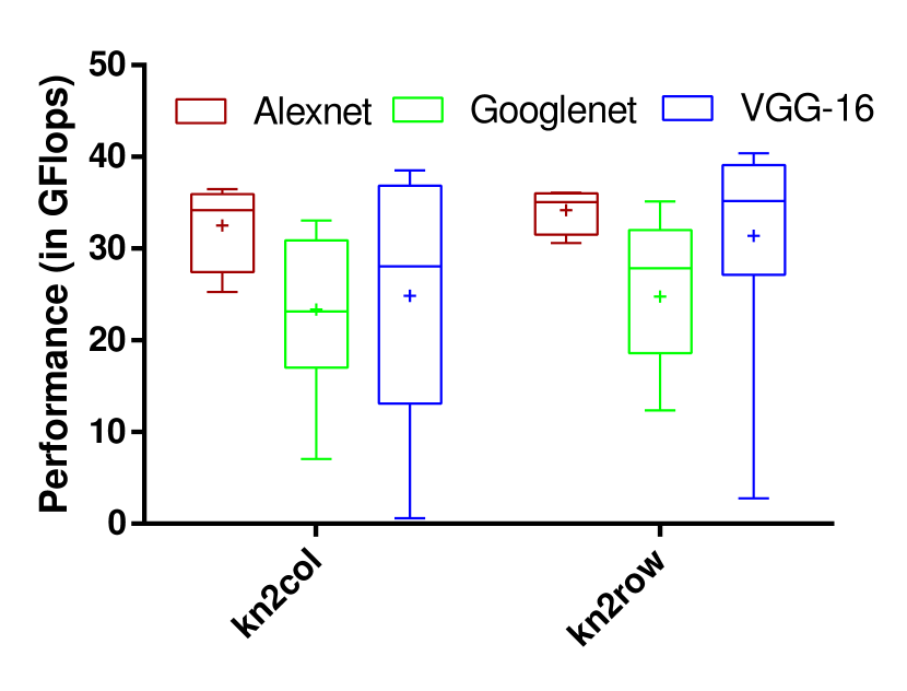
Figure 6: Performance of GEMM-based convolution with $O(K^{2})$ data growth in result matrix

Similar to figure 4, figure 6 compares the performance of the two kn2 methods from Vasudevan et al. [4]. The $kn2row$ method enjoys better locality and this is reflected in the performance delivered. The $kn2row$ also produces a slightly tighter spread of performance across layers in all the networks, most notably in AlexNet. Another interesting observation is that the performance of both $kn2col$ and $kn2row$ tend to increase with the $C$ and $M$ and decreases with the size of the kernel.

a0

a1

a2

a3

b0

b1

b2

b3

c0

c1

c2

c3

d0

d1

d2

d3

e0

e1

e2

e3

f0

f1

f2

f3

g0

g1

g2

g3

h0

h1

h2

h3

i0

i1

i2

i3

j0

j1

j2

j3

k0

k1

k2

k3

(a) Row-major linear layout of $11\times 4$ matrix

a0

a1

a2

a3

b0

b1

b2

b3

c0

c1

c2

c3

d0

d1

d2

d3

e0

e1

e2

e3

f0

f1

f2

f3

g0

g1

g2

g3

h0

h1

h2

h3

i0

i1

i2

i3

j0

j1

j2

j3

k0

k1

k2

k3

a0

a1

a2

a3

b0

b1

b2

b3

c0

c1

c2

c3

d0

d1

d2

d3

e0

e1

e2

e3

f0

f1

f2

f3

g0

g1

g2

g3

h0

h1

h2

h3

i0

i1

i2

i3

j0

j1

j2

j3

k0

k1

k2

k3

a0

a1

a2

a3

b0

b1

b2

b3

c0

c1

c2

c3

d0

d1

d2

d3

e0

e1

e2

e3

f0

f1

f2

f3

g0

g1

g2

g3

h0

h1

h2

h3

i0

i1

i2

i3

j0

j1

j2

j3

k0

k1

k2

k3

(b) The same data in memory reimagined in three different ways as $3\times 12$ matrices

Figure 7: A row-major $11\times 4$ matrix and three different ways to reimagine sub-ranges of the matrix as $3\times 12$ matrices. Note that the jagged parts at each end correspond to partial $3\times 12$ matrices. To perform convolution with these partial matrices, zero-padding must be added to each end of the original matrix.

Figure 8: Performance of GEMM-based convolution with $O(K)$ data growth

V GEMM-based Convolution with $O(KCHW)$ patch matrix

GEMM-based convolution can make very good use of the underlying hardware, but the method described in Section III requires a patch matrix with a factor of $K^{2}$ increase in the size of the input, and Section IV requires a $K^{2}$ increase in the output of the GEMM. In this section we describe an existing approach that requires just a factor of $K$ increase in the size of the input of the GEMM. This reduction in memory size is particularly welcome on memory-limited embeddes systems, but it can also improve locality and reduce memory traffic on other systems. Reducing memory traffic can be particularly important for multicore systems where all cores share a single interface to off-chip main memory.

V-A Reimagining matrix dimensions

Memory-Efficient Convolution (MEC) [11] is an extension of the classical $im2col$ which does not require a full $O(K^{2})$ patch matrix. The core idea of the algorithm relies on the layout of matrices in memory.

In C/C++ elements of a 1D array are contiguous in memory. A 2D array consists of a sequence of 1D arrays that are laid out contiguously in memory. Therefore, a 2D array with dimensions $H\times W$ has exactly the same layout in memory as a 1D array of size $HW$. Thus, we can switch between the two different interpretations of the data in memory by simply changing the type of the pointer to the array, without having to change the data in memory. It is this basic insight that allows the 2D GEMM algorithm to operate on multidimensional tensors in the all the algorithms presented in this paper.

Figure 7 shows a 2D $11\times 4$ matrix laid out contiguously in memory. It is possible to reinterpret a sub-region of this matrix as, say, a $3\times 12$ matrix without changing the layout in memory. By selecting different sub-regions, one can select different $3\times 12$ sub-matrices of the original. Using this mechanism, we can perform 1D convolution by selecting a sequence of $K$ rows of the matrix and treating them as a single row. The MEC algorithm [11] uses this approach to avoid having to create a patch matrix that is $O(K^{2})$ times the size of the original matrix. Instead MEC performs 1D convolutions by performing multiple GEMM operations on overlapping regions of the matrix. The MEC approach allows horizontal 1D convolutions to be performed without having to create a patch matrix, but the same trick cannot be used for vertical 1D convolutions, or indeed 2D convolutions.

To overcome this problem, the MEC algorithm creates a patch matrix that is $O(K)$ times the size of the original input to allow the vertical part of convolutions, and uses performs overlapping GEMMs for the horizontal part. The result is an algorithm that requires no more arithmetic operations than the classical $im2col$ algorithm, but requires only a factor of $O(K)$ times the input size in additional memory, rather than the $O(K^{2})$ required by $im2col$.

VI GEMM-based convolution with sub-$K$ data growth

The $kn2row$ algorithm eliminates the need for data replication in the input ($im2col$ requires a $K^{2}$ expansion of the input). However this results in a $K^{2}$ expansion in the result of the matrix multiplication. This problem might be thought of like a tube of toothpaste; if we squeeze the $K^{2}$ data expansion from the input image, it re-appears in the output of the matrix multiplication.

VI-A Accumulating $kn2row$ and $kn2col$

In order to avoid this “tube of toothpaste” problem, we introduce two new methods which are accumulating variants of $kn2row$ and $kn2col$ called Accumulating Kernel to Row ($kn2row-as$) and Accumulating Kernel to Column ($kn2col-as$) respectively. Instead of treating the kernel as one big kernel matrix of size $[K^{2}\times M]\times[C]$, the k2r-as accumulating method treats it as $K^{2}$ smaller $[M\times C]$ sized kernel matrices ($\mathcal{K}_{A}\cdots\mathcal{K}_{I}$) as shown in the Figure 9.

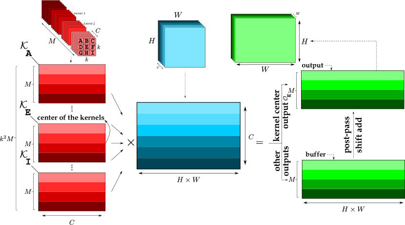
Figure 9: MCMK using the “$kn2row-as$” method

We then multiply the kernel $\mathcal{K}_{E}$ which corresponds to the center value of every channel of every kernel with the image matrix (shown in blue in the figure) of size $[C]\times[H\times W]$ which results in an output matrix ($\mathcal{O}_{E}$) of size $[M]\times[H\times W]$ which is stored in output directly without any shifting (as discussed in the section IV-A).

Kernel matrix $\mathcal{K}_{A}$ is then multiplied with the input matrix and the result is stored in buffer. Since the kernels in the figure are $3\times 3$, the row offset for the outputs produced by $\mathcal{K}_{A}$ is $+1$ and the corresponding column offset is also $+1$ as $E$ is one row down and column to the right of $A$. The values in buffer are shifted by the calculated offsets in its multi-channel representation. This process is repeated for the rest of the kernels ($\{\mathcal{K}_{B}\cdots\mathcal{K}_{I}\}-\{\mathcal{K}_{E}\}$). For a kernel of size $K\times K$ appropriate offset values are by calculating how far each value ($\mathcal{K}_{A}\cdots\mathcal{K}_{k^{2}}$) is away from the center of the kernel. Our $kn2col-as$ method works in the same way as $kn2row-as$, but with the input and kernel matrices transposed.

Figure 9 and its explanation in this section hold true for $kn2col-as$ along with applicable transformations to the kernels, inputs and outputs (as we have explained for converting $kn2row$ to $kn2col$).

VI-B Accumulating with GEMM

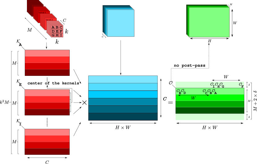
Figure 10: MCMK convolution using the accumulation that is built into the GEMM library call

The signature of GEMM in most BLAS libraries is $C=\alpha\times(A\ast B)+\beta\times C$. One can transform a GEMM call into an output accumulating GEMM, i.e. multiply the two input matrices $A$ and $B$ and add it to the resultant matrix $C$, by setting the value of the scalar parameter $\beta$ to zero. The k2r-aa method, leverages this output accumulating feature of GEMM as shown in Figure 10.

It works in the same way as $kn2row-as$ by treating the big kernel matrix of size $[K^{2}\times M]\times[C]$ as $K^{2}$ $[M\times C]$ smaller kernels ($\mathcal{K}_{A}\cdots\mathcal{K}_{I}$). To store the output, we reserve a contiguous piece of memory that is of size $[M+2\delta]\times[H\times W]$ where $\delta$ is the number of extra rows in the output matrix given by $\delta=\lceil\frac{K}{2H}\rceil$ for square kernel matrices.

Note that in the example in Figure 10 padding is added to the top and bottom of the result matrix which can be written to by the GEMM calls. The values computed in these padding array elements are never actually used. In the example, we have assumed that we always allocate full rows of size $HW$ for padding. If, however, we only allocate just enough array elements that are needed for padding rather than allocating full rows, then the additional space needed for padding is $O(KW)$.

A GEMM of $\mathcal{K}_{E}$ (corresponding to the center value of every channel of every kernel) and the input matrix produces an output matrix $\mathcal{O}_{E}$ as in Figure 10. Since this output corresponds to the center of the kernel, it does not have to be offset in the final output. If one were to add a similar output matrix $\mathcal{O}_{D}$ to the intermediate output then $\mathcal{O}_{D}$ has to be shifted to the right by one element as $\mathcal{D}$ is one element to the left of the center of the kernel. By the same logic, $\mathcal{O}_{F}$ has to be shifted left by one element as $\mathcal{F}$ is one element to the right of the center.

Thus, an element $\mathcal{X}$ in the kernel that is $x_{1}$ rows above the center and $y_{1}$ to the left of the center must be offset by $x_{1}\times W+y_{1}$. So we choose the starting location of the output associated with the first kernel ($\mathcal{K}_{A}$) such that the output corresponding to the center of the kernel will start at the start of the $\delta^{t}h$ row of the intermediate output. This starting address is given by $\mathcal{O}_{A}=\mathcal{O}_{t}+\lfloor\frac{K}{2}\rfloor(H\times W+W+1)$. Based on $\mathcal{O}_{A}$ and $\mathcal{O}_{E}$, we can calculate the rest of the starting addresses and supply them to successive accumulating GEMM calls. After $K^{2}$ GEMM calls have been made, the output starting at $\mathcal{O}_{E}$ denoted by $\mathcal{O}$ in Figure 10 contains the final output with correct accumulation of kernel and weight pairs.

Note that the final output $\mathcal{O}$ is a matrix of size $[M]\times[H\times W]$ starting at location $\mathcal{O}_{E}$. Therefore the edge pixels of the output are approximate values. At the boundaries of an image a convolution typically assumes that pixels outside of the image have a value of zero, but our Hole Punching Accumulating Kernel to Row ($kn2row-aa$) method instead takes the value from the opposite edge of the image.

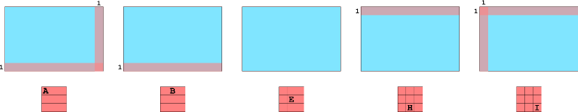
Figure 11: Hole punching in $kn2row-aa$

One way to fix this is by applying a post-pass where a loop based implementation of MCMK is applied to every erroneous error pixel. However, this has a significant impact on performance. In order to overcome the issue of producing correct results while being performant, we analyzed the pairs of products whose sum gave rise to the edge pixels in question.

Even though the right pairs of image pixels and kernel values are multiplied together, incorrect pairs are summed up together in the boundary pixels. As mentioned earlier, where image pixels are to be treated as zero (boundary handling) our $kn2row-aa$ reads the pixel values from the subsequent row in the opposite edge of the image due to the contiguous memory layout.

In order to avoid summing incorrect pairs of image pixels and kernel values, we propose an intermediate step between every GEMM call, that multiplies the an $K\times C$ kernel matrix (that corresponds to all the kernel values for a given position in a $K\times K$ kernel) with the $C\times[H\times W]$ image matrix. In this intermediate step we “punch holes” in the image matrix by setting certain positions of the image matrix to zero as shown in algorithm 11. The figure shows the regions that are zeroed out in a single channel of the input matrix for ease of understanding, but these regions are applicable for all channels in the input.

As discussed earlier, the intuition behind zeroing certain regions of the image before every accumulating GEMM call is to avoid unnecessary pairs of products being summed up together. For instance let’s consider the first part of figure 11 which corresponds to the GEMM of the input with the smaller kernel matrix ($\mathcal{K}_{A}$) corresponding to the A^th element. If convolution is performed with this element placed on a pixel of the input that is in the marked region, the center of the kernel falls outside the boundaries of the output thereby making this product of input and kernel unnecessary for the end result.

Similarly, for the B^th element, the last row of the input must be zeroed out. Note however, for the central element, no pixels need to be punched out because placing the E^th element on any pixel of the input will always result in the output of that convolution inside the boundary of the output. Between every GEMM call, we restore the pixels that were saved before the previous GEMM and save the pixels where “holes” are to be punched for the current GEMM call.

Figure 12 compares the performance of the accumulating versions of $kn2row$ and $kn2col$ described in section VI-A and the accumulating GEMM version with hole punching described in this section. The accumulating $kn2row$ ($kn2row-as$) and $kn2col$ ($kn2col-as$) perform much better compared to their baseline non-accumulating versions described in section IV. However, the two variants of the accumulating GEMM based hole-punching method harness the output data locality offered by having GEMM accumulate into offsetted output locations and seem to outperform the other accumulating methods.

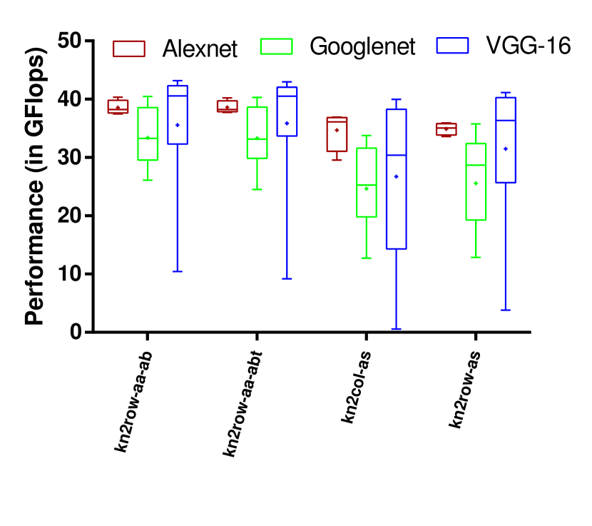
Figure 12: Performance of GEMM-based convolution with $O(<K)$ data growth

VII Results

VII-A Testing Environment

We evaluated the execution time of every previously mentioned convolution algorithm across a number of input dimensions. The input dimensions chosen were selected from three popular CNN architectures: AlexNet [12], VGG-16 [13], and GoogLeNet [10]. We chose these input dimensions as we believe they represent realistic inputs that the algorithms will be expected to handle when used for practical applications. We ran our experiments on two general-purpose processors, an Intel i7 and an ARM®Cortex®A57 (on a NVIDIA JTX1 board). We evaluated the speeds of all the algorithms executed on processors using both a single thread running on a single core, and using all the CPU cores allowing up to 8 threads on the i7 and 4 threads on the A57. The execution times measured the time needed to allocate and construct any intermediate data structures (e.g. the patch matrices for i2c and the extra output space for k2r), GEMM invocations and writing results to the output buffer. We did not measure the time needed to convert the input or output feature map to a specified format (i.e. we treated algorithms that produced outputs in $CxHxW$ format and $HxWxC$ format as equally valid).

On the i7 processor our algorithms were compiled using gcc 7.1.1 while on the A57 gcc 5.4.0 was used as it ships with the NVIDIA JTX1 board. We statically linked with the OpenBLAS library to implement GEMM. We used OpenBLAS version 0.2.2. We used OpenBLAS’ internal threading model to multithread the GEMM calls.

VII-B Memory Usage

Method	Label	Extra memory
im2row	im2row	$(K^{2}-1)\times((HW)\times C)$
im2col	im2col	$(K^{2}-1)\times((HW)\times C)$
Kernel to Row	kn2row	$(K^{2}-1)\times(M\times(HW))$
Kernel to Column	kn2col	$(K^{2}-1)\times(M\times(HW))$
Accumulating Kernel to Row	kn2row-as	$(H\times W)\times M$
Accumulating Kernel to Column	kn2col-as	$M\times(H\times W)$
Hole Punching Accumulating Kernel to Row	kn2row-aa	$K\times W$

TABLE I: Extra memory required

While evaluating our algorithms on the JTX1 board we found that for a number of our chosen input dimensions the board ran out of memory intermittetly while executing our $O(K^{2})$ algorithms. This occurred during the execution of the upper layers of VGG16 where we have a input feature map which is large in all dimensions. This demonstrates an area where the $O(K)$ and $O(<K)$ algorithms are particular necessary. The execution times for the problematic input dimensions have been omitted from the ARM result tables as the times for many of the $O(K^{2})$ algorithms could not be produced.

VII-C Resulting Trends

The general theme throughout the results we have observed points towards the fact that there is no one method to outperform them all. From this gamut of implementations of the convolution layer, there is seemingly no one method that is the pick of the lot. Instead, given a layer’s operating characteristics (i.e, number of channels $C$, kernels $M$, size of the kernel $K$ and input height $H$ and width $W$) most methods form clusters in their performance characteristics.

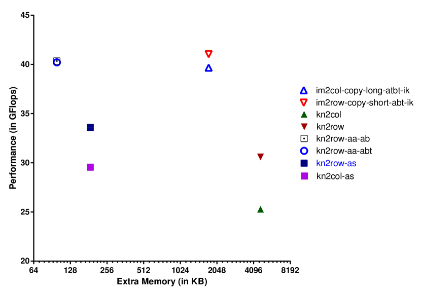
Figure 13: Performance vs extra memory required for all methods in conv2 of Alexnet

This is further illustrated by figures 13 and 14. Both these figures show the performance of a method compared against the extra memory required by each algorithm (in accordance with table I). Figure 13 is an instance of figure 14 as it shows the performance characteristics of selected methods for the second convolution layer of AlexNet while the latter represents all the methods and all the layers of AlexNet.

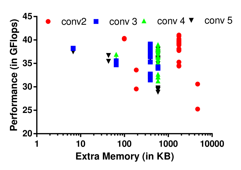
Figure 14: Performance vs extra memory required for all the methods in all layers of Alexnet

It is very evident from figure 13 that the non-accumulating kn2 methods require the most extra memory for the second convolution layer of AlexNet while providing low performance. However their accumulating counterparts require nearly $\dfrac{1}{20}^{th}$ the extra memory required while providing better runtimes. The im2 methods represented here are the best performing out of the gamut of methods presented in section IV. The hole-punching methods ($kn2row-aa$) are competent compared to the im2 methods while requiring the least amount of extra memory.

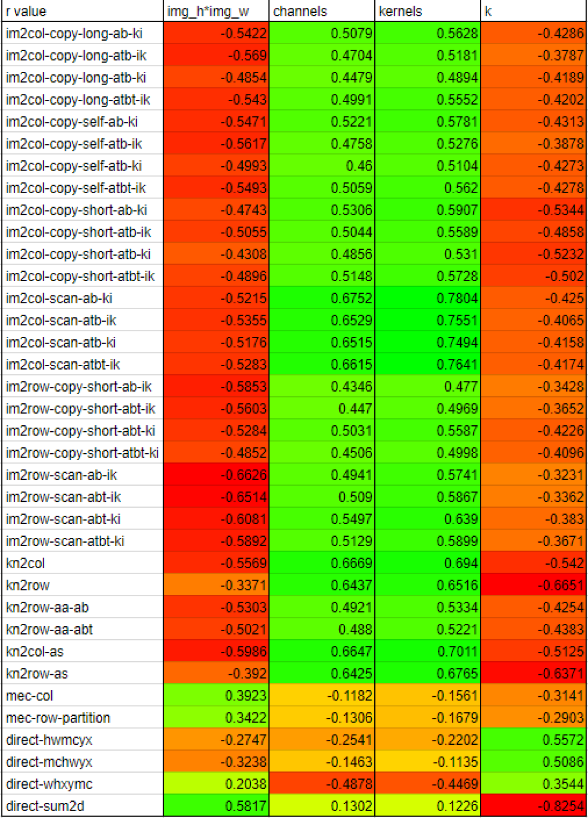
Figure 15: Correlation matrix of all methods vs convolution parameters

Figure 15 shows the the correlation coefficient between each of the operating condition variables (i.e, number of channels $C$, kernels $M$, size of the kernel $k$ and input height times width $H\times W$). It is interesting to note that all the GEMM based methods have a positive correlation with the number of channels and number of kernels while they have a negative correlation with the number of pixels in the image and the size of the kernel.

The non-accumulating kn2 methods have a worse negative correlation with the number of kernels, i.e. as the number of kernels tend to increase the performance tends to decrease which is explained by the fact that the size of the result matrix grows (along one direction; either rows or columns increase) as $k$ increases thereby resulting in a GEMM between oddly shaped matrices. The accumulating versions of the kn2 methods have an even worse effect as the number of distinct GEMM calls increases quadratically with $k$.

The $O(K)$ data growth methods have a positive correlation with the number of pixels in the input and a negative correlation with the number of channels and kernels. We have also added the direct loop based methods as described in figure 1. The suffixes for these methods indicate the loop ordering from the figure.

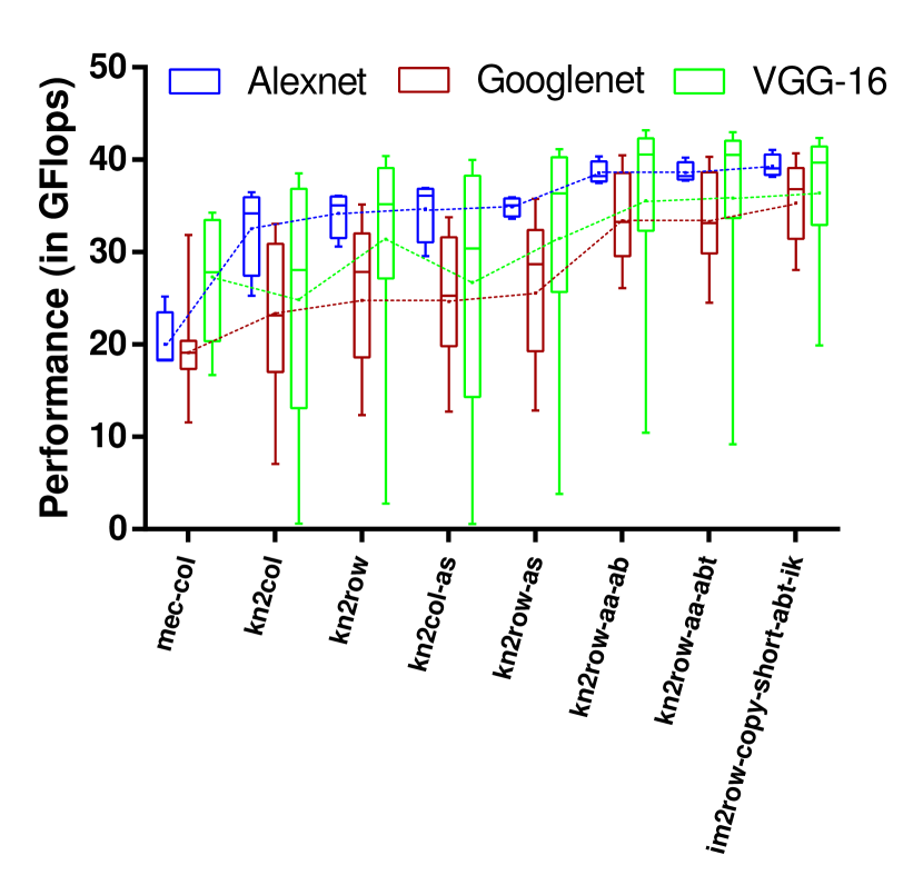
Figure 16: Performance of the best GEMM-based convolutions for AlexNet, GoogLeNet and VGG-16

These graphs clearly show that there is a wide range of performance characteristics displayed by the methods discussed in this paper. The ramifications of this are two-fold: (1) user’s choice is paramount as the choice of implementations depend on the deployment environment, i.e. for a mobile based deployment scenario, the hole-punching methods are seemingly the correct choice as they require the least overhead in memory requirement and are competent with the other methods in terms of performance and (2) the optimal choice of implementations and layouts to minimize the total execution time of a network posits a complicated optimization problem.

VII-D Other Experiments

We also implemented versions of our algorithms that used OpenMP to parallelize the data transformations needed to construct the intermediate data structures in $im2col$, $im2row$ and Memory-Efficient Convolution (MEC). However we found that the speed improvements from this were negilible. We used OpenMP 4.0.1-1 and allowed eight threads on the i7 processor and 4 threads on the A57.

We also measured the number of stall cycles that occurred due to L1 and L3 cache while running our tabled experiments on the i7 processor. We found that the optimal version of k2r (labeled kn2row-aa in the tables) had on average the least number of stall cycles, although for the upper layers of VGG16 MEC fared best. This falls in line with the execution times recorded on the i7 processor.

VIII Related Work

The $im2col$ method of performing MCMK is an extension of well-known methods of performing 2D convolution using a Toeplitz matrix. Chellapilla et al. [5] are the first researchers to implement MCMK using using $im2col$. They report significant speedups compared to the simpler approach of summing multiple channels of 2D convolutions.

Yanqing et al. rediscovered $im2col$ for the Caffe deep learning system [9], which uses GPUs and other accelerators to speed up Deep Neural Networks (DNNs). The $im2col$ approach remains the most widely-used way to implement MCMK, and is used in deep learning frameworks such as Caffe, Theano and Torch.

Gu et al. [14] apply $im2col$ to a batch input images to create a column matrix for multiple input images. They find that batching can improve throughput by better matching the input matrix sizes to the optimal sizes for their GEMM library.

Tsai et al. [15] present a set of configurable OpenCL kernels for MCMK. By coding the MCMK loop nests directly they eliminate the need for $im2col$ data replication, and thus allow the use of larger batch sizes while maintaining constraints on local memory. The found that the performance of a naive loop nest for MCMK is not good, but they achieve satisfactory performance with a program generator and autotuner.

Chetlur et al. [16] propose a GEMM-based approach to convolution based on $im2col$. However, rather than creating the entire column matrix in one piece, they instead lazily create sub-tiles of the column matrix in on-chip memory. To optimize performance, they match the size of their sub-matrix tiles to the tile sizes used by the underlying GEMM implementation. They find that this lazy $im2col$ achieves speedups over Caffe’s standard $im2col$ of between around 0% and 30%.

IX Conclusion

Multi-channel multi-kernel convolution is the most computationally expensive operation in DNNs. Maximal exploitation of processor resources for MCMK requires a deep understanding of the micro-architecture. Careful design of data blocking strategies to exploit caches, on-chip memories and register locality are needed, along with careful consideration of data movement and its interaction with SIMD/SIMT parallelism. Each new processor has different performance characteristics, requiring careful tuning of the code each time it is brought to a new target.

There are significant advantages in implementing MCMK convolution using existing carefully tuned General Matrix Multiplication (GEMM) libraries. However, the most widely-used approach, $im2col$ has a large memory footprint because it expands the input image to a much larger patch matrix. This space expansion is quadratic in the order, $K$, of the 2D convolution being performed. This is problematic for memory-constrained systems such as embedded object detection and recognition systems. Additionally, the data redundancy resulting from $im2col$ reduces data locality and increases memory traffic.

We propose two new approaches for implementing MCMK convolution using existing parallel GEMM libraries that require much less memory. These algorithms dramatically reduce the space overhead of DNN convolution, making it much more suitable for memory-limited embedded systems. These algorithms replace the single GEMM call of the $K^{2}$ patch-building approaches with an accumulation of the result of $K^{2}$ different $1\times 1$ convolutions. The result is a dramatic reduction in memory requirements and improved data locality.

Experimental evaluation shows that our low-memory algorithms are just as fast as the best patch-building approaches despite requiring just a fraction of the amount of additional memory. Our low-memory algorithms have excellent data locality which gives them a further edge over patch-building algorithms when multiple cores are used. As a result, our low memory algorithms often outperform the best patch-building algorithms using multiple threads.

height	27	13	13	13	57	57	28	28	14	7	224	224	112	112	56	56	28	28	14	14
width	27	13	13	13	57	57	28	28	14	7	224	224	112	112	56	56	28	28	14	14
channels	96	256	384	384	64	64	16	96	160	832	3	64	64	128	128	256	256	512	512	1024
k	5	3	3	3	1	1	5	3	3	1	3	3	3	3	3	3	3	3	3	3
kernels	256	384	384	256	64	192	32	128	320	384	64	64	128	128	256	256	512	512	1024	1024
im2col-copy-long-ab-ki	21.13	7.135	10.71	7.331	0.804	2.073	0.666	4.001	4.079	0.923	7.217	122.4	48.79	97.38	43.09	85.88	40.01	80.27	40.90	81.98
im2col-copy-long-atb-ik	20.51	7.082	10.64	7.256	0.806	2.101	0.663	4.186	4.238	0.913	7.733	122.4	48.90	98.06	42.24	84.26	40.23	80.75	42.32	84.26
im2col-copy-long-atb-ki	21.22	7.316	11.11	7.484	0.797	2.091	0.654	4.054	4.189	0.980	7.209	122.1	48.10	97.42	42.53	85.85	40.52	81.10	42.98	86.10
im2col-copy-long-atbt-ik	20.36	7.007	10.53	7.198	0.794	2.091	0.701	4.193	4.217	0.886	7.760	122.4	48.67	98.33	42.59	84.37	39.92	79.84	41.01	83.48
im2col-copy-self-ab-ki	21.11	7.105	10.72	7.313	0.924	2.155	0.666	4.051	4.097	0.925	7.201	123.2	48.78	98.20	43.09	86.09	39.97	79.76	40.95	82.06
im2col-copy-self-atb-ik	20.41	7.059	10.70	7.275	0.904	2.154	0.698	4.216	4.228	0.906	7.719	123.1	48.87	98.48	42.35	85.13	40.45	80.57	42.11	84.58
im2col-copy-self-atb-ki	21.25	7.314	11.15	7.502	0.911	2.151	0.659	4.089	4.223	0.946	7.197	123.1	48.89	97.80	43.44	86.15	40.20	81.54	42.95	86.13
im2col-copy-self-atbt-ik	20.44	7.005	10.50	7.224	0.892	2.154	0.682	4.227	4.211	0.913	7.756	123.2	48.77	98.39	42.68	85.17	40.05	79.94	41.07	83.84
im2col-copy-short-ab-ki	21.32	7.116	10.69	7.298	0.857	2.122	0.686	4.033	4.080	0.900	7.212	123.4	48.22	97.78	43.01	84.96	40.11	80.23	40.84	81.89
im2col-copy-short-atb-ik	20.59	7.098	10.63	7.246	0.821	2.141	0.699	4.130	4.220	0.885	7.724	122.9	48.52	98.28	42.57	85.07	40.42	80.25	42.08	84.24
im2col-copy-short-atb-ki	21.53	7.344	11.08	7.470	0.797	2.119	0.733	4.033	4.193	0.941	7.226	123.1	48.12	98.05	43.50	85.38	40.48	80.26	42.90	86.02
im2col-copy-short-atbt-ik	20.63	6.991	10.49	7.150	0.831	2.102	0.709	4.146	4.186	0.930	7.775	123.2	48.68	98.54	42.73	85.02	39.84	80.15	40.92	83.77
im2col-scan-ab-ki	23.36	8.480	12.55	9.147	6.294	7.523	1.191	6.236	5.067	2.039	11.03	218.0	69.38	142.5	54.48	108.7	45.40	92.34	43.69	87.81
im2col-scan-atb-ik	22.81	8.291	12.56	9.126	6.266	7.497	1.191	6.153	5.042	2.071	11.54	218.1	69.08	143.0	54.37	108.4	45.71	92.52	44.90	90.40
im2col-scan-atb-ki	23.50	8.561	12.94	9.381	6.296	7.510	1.195	6.257	5.175	2.125	11.02	216.9	69.30	142.8	54.73	109.2	46.08	93.12	45.77	91.86
im2col-scan-atbt-ik	22.71	8.264	12.36	9.057	6.281	7.509	1.150	6.236	5.111	2.047	11.56	217.3	69.50	143.6	54.19	107.5	45.22	92.00	44.05	89.80
im2row-copy-short-ab-ik	19.71	6.926	10.54	7.088	0.759	2.044	0.635	3.960	4.034	0.890	8.021	113.2	46.80	91.79	41.30	82.44	39.52	78.82	42.08	84.17
im2row-copy-short-abt-ik	19.62	6.924	10.37	7.074	0.784	2.049	0.631	3.987	4.062	0.887	7.981	113.1	46.70	91.95	41.12	82.40	39.25	78.92	40.73	83.54
im2row-copy-short-abt-ki	20.23	7.125	10.69	7.297	0.839	2.167	0.681	4.206	4.185	0.934	8.292	117.4	47.24	93.92	41.94	83.00	39.25	78.52	40.68	81.77
im2row-copy-short-atbt-ki	20.34	7.310	11.10	7.468	0.821	2.165	0.729	4.225	4.281	0.959	7.834	117.6	47.71	94.30	42.03	83.07	39.94	79.92	42.73	85.85
im2row-scan-ab-ik	20.12	7.123	10.81	7.408	1.360	2.593	0.730	4.349	4.259	0.885	8.372	158.1	53.11	109.2	44.49	89.48	40.92	82.64	42.77	85.94
im2row-scan-abt-ik	20.14	7.185	10.73	7.444	1.237	2.569	0.683	4.337	4.219	0.927	8.301	155.8	52.47	107.6	43.84	88.52	40.57	82.03	41.71	84.95
im2row-scan-abt-ki	20.62	7.410	11.04	7.663	1.346	2.624	0.750	4.577	4.354	0.901	8.121	160.0	53.00	109.6	44.75	90.13	40.83	82.36	41.39	83.66
im2row-scan-atbt-ki	20.87	7.645	11.46	7.862	1.341	2.644	0.757	4.614	4.459	0.984	8.255	160.4	53.41	110.0	44.91	90.06	41.08	82.80	43.46	87.61
kn2col	32.48	7.977	11.77	7.452	1.104	3.047	2.561	5.416	4.978	0.929	272.7	340.8	117.8	158.5	63.20	97.16	48.79	86.81	46.35	88.49
kn2col-as	27.21	7.577	10.92	7.317	1.117	2.935	1.446	5.495	4.823	0.890	307.0	384.7	80.04	127.3	53.49	93.87	44.46	83.00	44.01	85.62
kn2row	26.70	7.798	11.30	7.445	0.857	2.362	1.234	4.707	4.846	0.904	60.87	126.4	63.09	99.45	48.49	85.11	43.37	82.72	44.30	84.15
kn2row-aa-ab	19.74	6.995	10.45	7.086	0.761	1.902	0.676	4.029	4.105	0.903	15.95	113.8	47.52	94.76	39.75	81.55	38.16	76.82	40.70	80.28
kn2row-aa-abt	19.87	7.016	10.51	7.126	0.752	1.923	0.738	4.068	4.120	1.015	16.45	104.0	45.65	87.85	39.60	78.50	38.28	76.95	40.81	80.65
kn2row-as	23.83	7.860	11.21	7.586	0.846	2.131	1.194	4.758	4.762	0.901	44.26	143.5	62.01	107.4	47.31	90.48	41.23	80.11	42.76	82.20
mec-col	32.00	14.52	21.74	14.80	1.164	2.667	0.890	6.093	8.397	2.474	6.852	101.9	48.75	96.43	50.64	101.5	59.87	124.4	90.44	199.5
mec-row-partition	31.77	14.51	21.69	14.60	1.021	2.482	0.829	5.929	8.334	2.516	7.197	107.0	48.73	97.28	50.40	101.7	59.90	125.1	91.01	199.4

(a) single-threaded

im2col-copy-long-ab-ki	7.946	3.230	5.094	3.348	0.738	0.667	0.554	1.447	1.716	1.296	4.282	64.99	24.12	61.82	15.58	29.74	13.61	27.02	16.55	33.51
im2col-copy-long-atb-ik	7.267	2.773	4.060	2.953	0.427	0.784	0.408	1.558	1.458	0.412	9.306	103.8	26.89	52.41	15.48	30.07	12.83	25.81	13.55	26.77
im2col-copy-long-atb-ki	7.778	3.285	5.068	3.401	0.284	0.671	0.556	1.445	2.187	0.904	4.271	65.07	23.66	61.72	15.64	29.80	13.62	27.12	17.36	34.92
im2col-copy-long-atbt-ik	7.397	2.740	3.999	2.924	0.383	0.801	0.421	1.469	1.880	0.627	9.312	104.2	26.93	52.33	15.93	30.21	13.01	25.80	13.31	27.09
im2col-copy-self-ab-ki	7.788	3.250	4.897	3.334	0.478	0.842	0.582	1.514	1.722	0.897	4.310	68.03	24.60	63.12	16.11	30.30	13.60	26.92	16.59	33.54
im2col-copy-self-atb-ik	7.261	2.754	3.837	2.968	0.619	0.964	0.435	1.557	1.426	0.409	9.394	106.5	27.53	53.82	15.95	30.53	13.17	26.00	13.53	26.81
im2col-copy-self-atb-ki	7.846	3.285	6.020	3.428	0.474	0.836	0.591	1.801	1.969	0.908	4.347	67.41	24.34	62.02	16.27	30.66	14.05	27.43	17.38	34.82
im2col-copy-self-atbt-ik	7.244	2.727	3.851	2.879	0.577	0.953	0.436	2.070	1.440	0.414	9.389	106.5	27.76	53.83	16.37	30.93	13.27	25.95	13.29	26.75
im2col-copy-short-ab-ki	8.218	3.202	5.048	3.336	0.283	0.666	0.634	1.948	1.687	0.886	4.322	66.15	23.77	62.12	15.46	29.84	13.50	27.50	16.57	33.89
im2col-copy-short-atb-ik	7.479	2.762	4.057	2.944	0.387	0.781	0.511	1.792	1.713	0.420	9.323	105.0	26.96	53.33	15.89	30.40	12.93	25.51	13.47	27.04
im2col-copy-short-atb-ki	8.099	3.279	5.173	3.359	0.282	0.666	0.878	1.912	2.160	1.096	4.300	66.67	23.91	61.88	15.82	29.86	13.68	27.03	17.48	34.65
im2col-copy-short-atbt-ik	7.581	2.737	3.943	2.886	0.417	0.781	0.490	1.999	1.410	0.846	9.389	104.9	26.75	52.55	15.66	30.35	12.94	25.73	13.24	26.98
im2col-scan-ab-ki	14.23	6.784	9.784	8.531	13.99	14.44	1.839	7.133	4.095	3.707	15.82	273.3	80.56	161.4	45.02	92.92	27.94	56.92	24.18	48.67
im2col-scan-atb-ik	13.72	6.010	8.722	7.695	14.14	14.54	2.002	7.005	3.811	3.199	20.86	310.2	83.30	154.4	45.35	93.78	27.27	56.11	21.05	42.23
im2col-scan-atb-ki	14.33	6.768	9.868	8.371	14.04	14.46	1.850	7.142	4.270	4.038	15.83	272.4	80.78	163.2	44.78	93.83	27.98	57.47	24.86	50.06
im2col-scan-atbt-ik	13.67	5.976	8.834	7.760	14.13	14.57	1.882	7.297	3.942	3.176	20.86	309.9	84.23	154.6	45.17	94.23	27.35	56.12	20.77	42.13
im2row-copy-short-ab-ik	6.994	2.703	3.979	2.845	0.378	0.773	0.866	1.469	1.422	0.612	10.16	102.1	26.03	52.03	15.76	30.65	12.70	25.21	13.48	26.72
im2row-copy-short-abt-ik	6.970	2.635	3.949	2.839	0.492	0.777	0.647	1.455	1.374	0.395	10.26	102.0	26.15	51.98	15.59	30.69	12.72	25.20	12.99	26.68
im2row-copy-short-abt-ki	7.714	3.246	5.052	3.339	0.296	0.676	0.349	1.423	1.661	1.274	4.926	66.85	23.83	60.39	15.64	30.67	13.35	26.32	16.80	33.51
im2row-copy-short-atbt-ki	7.842	3.241	5.262	3.395	0.730	0.972	0.349	1.453	1.691	0.905	4.971	68.23	23.99	61.82	15.91	30.94	13.49	26.93	17.32	34.98
im2row-scan-ab-ik	7.674	2.900	4.400	3.209	0.963	1.326	0.571	2.247	1.744	0.429	10.44	147.5	33.81	70.41	19.77	40.93	15.01	30.57	14.32	28.82
im2row-scan-abt-ik	7.776	3.078	4.550	3.403	0.893	1.315	0.944	2.599	2.071	0.410	10.26	147.0	34.16	70.17	19.10	37.89	14.63	30.00	14.06	28.99
im2row-scan-abt-ki	8.392	3.665	5.637	3.873	0.802	1.457	0.468	2.230	2.357	0.904	4.972	111.0	31.10	75.24	19.27	37.98	15.24	30.56	17.45	35.65
im2row-scan-atbt-ki	8.593	3.897	5.729	4.190	0.827	1.353	0.763	2.333	2.249	0.965	4.988	112.2	30.48	79.78	19.38	37.80	15.31	30.96	18.32	37.15
kn2col	24.06	3.915	6.040	3.799	0.737	2.050	2.438	3.843	2.837	0.849	281.5	295.2	118.5	130.3	40.30	50.55	26.57	38.65	21.79	39.59
kn2col-as	17.67	3.535	4.644	3.169	0.741	1.938	1.854	3.595	2.874	0.408	376.6	453.2	69.82	121.9	32.39	47.41	20.84	32.93	17.11	30.50
kn2row	16.39	4.575	6.248	4.170	0.341	1.051	1.027	2.351	2.800	1.185	67.78	74.16	36.82	48.19	23.97	34.48	19.80	32.64	23.70	41.40
kn2row-aa-ab	7.064	3.185	4.646	3.418	0.239	0.666	0.308	1.572	1.694	0.873	15.16	37.85	15.91	31.53	12.09	25.10	12.39	24.78	16.61	32.82
kn2row-aa-abt	7.345	3.171	4.613	3.211	0.250	0.655	0.327	1.620	1.985	0.868	15.01	34.21	15.38	29.17	12.02	25.46	12.88	25.64	16.59	33.23
kn2row-as	11.99	4.241	5.714	4.123	0.266	0.731	0.956	2.426	2.645	1.079	45.06	71.02	30.43	47.81	19.40	35.45	16.08	28.77	19.88	36.64
mec-col	32.11	14.51	21.78	14.82	1.144	1.420	1.675	7.647	8.416	2.465	5.394	51.75	22.80	43.65	20.50	40.38	60.38	124.5	90.77	200.6
mec-row-partition	31.87	15.81	22.39	15.87	1.903	1.217	1.608	8.471	10.27	4.075	7.132	59.92	24.04	47.01	20.81	41.76	59.20	125.0	91.03	200.5

(b) multi-threaded

TABLE II: Execution times (ms) on an Intel i7. Red is fastest, orange is second fastest, yellow is third fastest.

height	27	13	13	13	57	57	28	28	14	7	56	56	28	28	14	14
width	27	13	13	13	57	57	28	28	14	7	56	56	28	28	14	14
channels	96	256	384	384	64	64	16	96	160	832	128	256	256	512	512	1024
k	5	3	3	3	1	1	5	3	3	1	3	3	3	3	3	3
kernels	256	384	384	256	64	192	32	128	320	384	256	256	512	512	1024	1024
im2col-copy-long-ab-ki	87.43	30.51	47.21	30.37	3.815	9.266	2.280	17.63	17.57	3.434	170.7	343.8	173.1	346.9	177.9	358.9
im2col-copy-long-atb-ik	94.03	30.78	46.98	31.63	3.796	9.726	2.407	18.95	18.20	3.331	186.2	364.1	176.3	358.6	174.6	356.3
im2col-copy-long-atb-ki	92.08	33.97	46.76	34.04	3.809	9.247	2.338	18.04	18.25	3.601	169.2	340.1	175.5	350.1	189.1	380.8
im2col-copy-long-atbt-ik	91.87	30.62	46.42	33.15	3.736	10.00	2.437	18.37	17.56	3.325	183.2	368.3	181.4	353.3	176.0	365.9
im2col-copy-self-ab-ki	94.94	30.21	45.41	30.36	4.027	9.400	2.374	18.93	18.31	3.546	178.7	341.3	173.1	350.1	176.6	355.9
im2col-copy-self-atb-ik	94.23	30.26	46.59	31.75	3.922	9.391	2.777	18.56	18.35	3.298	184.7	366.2	177.6	366.4	174.2	356.6
im2col-copy-self-atb-ki	100.3	31.62	47.41	32.48	3.971	9.729	2.345	18.07	18.28	3.590	172.0	343.5	175.4	352.8	187.4	375.4
im2col-copy-self-atbt-ik	96.57	29.96	45.53	31.32	3.905	9.561	2.447	18.85	17.82	3.363	187.2	371.2	178.7	355.3	175.9	359.6
im2col-copy-short-ab-ki	86.44	30.04	44.69	31.23	3.808	9.369	2.297	17.45	17.86	3.836	170.0	337.2	171.8	345.3	175.7	359.8
im2col-copy-short-atb-ik	90.47	30.63	45.82	31.80	3.738	9.282	2.539	18.50	17.76	3.375	181.3	369.2	176.6	355.9	175.0	352.7
im2col-copy-short-atb-ki	87.12	31.10	46.69	31.70	3.867	9.224	2.292	19.12	20.81	3.702	169.9	342.9	174.1	350.3	185.7	379.9
im2col-copy-short-atbt-ik	90.79	29.85	45.13	30.68	4.023	9.236	2.449	18.03	17.37	3.361	184.1	367.9	174.9	359.4	175.8	366.4
im2col-scan-ab-ki	105.3	39.04	59.40	44.90	32.41	37.78	4.563	30.08	23.95	10.45	236.6	494.0	205.9	412.0	196.2	401.8
im2col-scan-atb-ik	109.9	39.88	58.62	45.81	32.82	38.69	4.832	31.43	23.08	9.062	253.1	505.4	210.9	427.0	193.0	387.7
im2col-scan-atb-ki	106.1	47.51	61.98	44.93	32.62	37.79	4.707	30.54	24.27	9.457	238.0	478.9	210.1	425.4	205.6	414.0
im2col-scan-atbt-ik	109.3	39.73	58.05	44.17	33.77	37.48	5.414	30.79	23.34	9.258	251.4	516.4	215.5	424.0	194.0	398.0
im2row-copy-short-ab-ik	86.39	29.70	45.64	29.67	3.597	9.104	2.248	17.23	17.23	3.381	178.8	352.9	173.1	348.4	172.1	346.4
im2row-copy-short-abt-ik	85.69	29.09	43.63	29.86	3.443	9.041	2.195	18.67	16.88	3.311	181.4	359.0	173.8	356.5	173.6	350.4
im2row-copy-short-abt-ki	85.36	30.11	44.35	33.19	3.993	9.369	2.234	17.67	18.43	3.339	171.6	340.7	170.3	345.9	175.0	352.2
im2row-copy-short-atbt-ki	86.54	30.78	47.38	32.39	3.994	9.459	2.334	17.74	18.38	3.440	172.0	336.5	174.0	357.8	185.9	371.2
im2row-scan-ab-ik	91.53	30.36	45.54	31.11	5.414	11.93	3.802	19.01	17.94	3.476	189.9	384.7	179.0	361.5	174.5	350.5
im2row-scan-abt-ik	91.89	30.54	45.41	32.41	4.924	10.70	3.097	18.29	17.81	3.644	189.3	389.0	176.8	365.8	175.8	354.2
im2row-scan-abt-ki	90.93	29.91	46.11	30.20	5.376	10.93	3.122	18.37	17.38	3.442	181.5	374.2	175.8	356.8	176.0	355.8
im2row-scan-atbt-ki	91.21	31.24	49.26	33.37	5.286	10.97	3.125	18.74	18.08	3.733	181.2	374.6	178.4	366.2	187.3	374.1
kn2col	131.7	32.33	45.22	30.00	4.162	13.38	7.109	23.47	22.28	3.248	501.6	672.3	208.3	368.7	186.8	356.8
kn2col-as	123.5	34.35	48.51	32.85	4.794	14.73	5.755	21.75	20.86	3.212	336.8	521.7	215.7	393.4	193.5	364.2
kn2row	109.4	34.99	48.10	32.56	3.742	10.59	4.739	20.75	19.64	3.207	196.5	358.8	188.8	367.8	189.2	363.3
kn2row-aa-ab	90.84	30.76	47.07	34.30	3.370	9.231	2.252	16.07	17.43	3.731	176.5	362.1	179.5	353.7	186.8	356.2
kn2row-aa-abt	90.20	31.14	48.21	29.95	3.580	9.425	2.309	16.52	18.08	3.998	177.9	355.3	179.8	352.9	185.2	354.9
kn2row-as	102.6	32.92	47.04	32.32	3.469	9.226	3.143	18.28	18.81	3.321	189.0	359.7	188.5	362.0	188.5	361.1
mec-col	120.5	49.11	72.45	47.76	4.677	11.34	2.810	20.22	25.58	7.009	191.6	399.9	218.1	448.9	299.0	653.1
mec-row-partition	118.1	47.85	80.21	47.43	4.336	10.18	2.300	18.97	25.54	6.237	194.1	394.3	218.6	437.7	298.8	647.9

(a) single-threaded

im2col-copy-long-ab-ki	29.79	11.30	17.08	10.96	1.220	2.889	0.852	5.858	6.322	1.276	54.42	116.3	57.96	110.2	55.36	112.5
im2col-copy-long-atb-ik	30.27	10.22	15.29	12.16	1.322	3.357	1.052	6.138	6.118	1.294	58.90	119.4	60.25	114.5	58.07	121.1
im2col-copy-long-atb-ki	30.98	10.46	16.03	11.27	1.194	2.947	0.897	6.229	6.371	1.314	56.20	114.6	56.68	110.6	57.14	118.2
im2col-copy-long-atbt-ik	33.05	10.70	15.40	12.18	1.342	3.357	1.161	6.220	6.070	1.711	59.75	121.9	59.02	114.5	56.52	120.7
im2col-copy-self-ab-ki	31.25	10.29	15.86	10.98	1.397	2.890	0.915	6.038	5.902	1.279	59.18	118.2	57.64	110.7	53.42	112.8
im2col-copy-self-atb-ik	30.68	12.16	15.97	11.10	1.340	3.445	1.209	6.368	6.337	1.307	60.94	122.7	58.63	117.8	57.67	118.5
im2col-copy-self-atb-ki	31.25	10.61	16.07	11.50	1.373	2.880	0.915	6.603	6.148	1.374	56.59	116.9	58.80	112.7	55.63	128.6
im2col-copy-self-atbt-ik	30.62	10.17	15.55	11.18	1.435	3.573	1.247	6.337	6.042	1.277	59.97	124.3	58.79	117.1	59.24	116.8
im2col-copy-short-ab-ki	29.96	9.855	15.06	12.03	1.188	2.830	0.839	5.592	5.705	1.292	54.69	118.4	54.97	110.5	53.84	113.9
im2col-copy-short-atb-ik	29.81	10.00	15.38	10.76	1.343	3.349	1.098	6.767	5.938	1.314	58.08	119.1	58.53	114.8	57.30	145.8
im2col-copy-short-atb-ki	31.17	10.20	16.98	10.92	1.225	2.795	0.851	5.528	5.876	1.352	53.42	113.7	55.82	110.6	56.22	116.3
im2col-copy-short-atbt-ik	29.65	10.20	14.75	10.51	1.326	3.352	1.538	6.007	5.819	1.273	57.47	118.6	59.23	118.0	57.09	116.4
im2col-scan-ab-ki	49.49	19.48	29.75	25.68	29.71	30.86	3.212	19.03	11.31	6.926	120.9	248.1	90.13	180.8	72.53	151.4
im2col-scan-atb-ik	48.29	19.29	28.54	24.05	29.57	32.48	3.764	19.04	11.39	7.629	124.6	255.5	92.44	184.3	77.37	156.1
im2col-scan-atb-ki	49.56	19.02	30.32	24.13	29.59	30.78	3.252	18.34	11.48	7.086	121.8	249.4	89.46	180.5	76.32	156.4
im2col-scan-atbt-ik	48.99	18.51	30.47	23.67	30.48	31.68	3.536	18.51	11.63	7.020	124.7	256.0	90.68	187.6	76.87	158.9
im2row-copy-short-ab-ik	30.09	9.770	14.80	10.38	1.130	3.285	1.031	5.592	5.816	1.270	56.67	120.6	59.23	114.4	56.50	115.2
im2row-copy-short-abt-ik	29.38	10.40	14.78	10.64	1.259	3.305	1.026	5.775	5.904	1.223	58.58	117.2	57.92	114.2	58.28	115.6
im2row-copy-short-abt-ki	29.37	11.04	15.00	11.83	1.356	2.938	0.859	5.518	6.204	1.231	53.35	114.3	55.53	109.0	52.98	110.2
im2row-copy-short-atbt-ki	28.18	11.25	16.84	11.27	1.262	2.832	0.848	5.557	6.073	1.339	53.76	116.5	58.11	111.2	57.72	116.4
im2row-scan-ab-ik	35.67	10.54	15.98	11.69	16.39	6.532	3.082	7.153	6.347	1.427	71.81	159.5	75.56	125.7	62.03	120.7
im2row-scan-abt-ik	33.67	10.36	16.23	11.28	2.894	4.835	1.732	7.799	6.125	1.386	69.77	156.4	65.23	125.9	58.78	119.4
im2row-scan-abt-ki	34.30	10.60	17.46	12.65	3.642	4.275	1.554	6.653	7.185	1.428	67.70	160.0	62.30	118.3	56.88	113.8
im2row-scan-atbt-ki	34.59	10.81	17.14	11.89	2.917	4.378	1.458	6.771	6.205	1.502	67.43	149.0	60.96	121.7	58.73	120.2
kn2col	67.26	13.86	18.38	13.40	2.238	7.810	4.874	12.70	9.116	1.204	374.8	430.7	90.76	141.6	71.27	128.0
kn2col-as	59.39	13.66	17.86	11.40	2.172	7.628	4.468	11.12	9.873	1.194	192.8	252.2	95.45	145.1	67.29	123.8
kn2row	42.41	12.03	16.32	12.44	1.126	3.820	2.593	7.561	7.210	1.219	72.83	128.6	65.08	115.2	62.01	117.3
kn2row-aa-ab	26.75	8.722	13.26	9.605	0.915	2.694	0.813	4.625	5.461	1.186	54.18	113.8	55.62	106.3	53.74	105.9
kn2row-aa-abt	24.46	8.732	14.36	9.269	0.925	6.723	0.677	4.619	4.674	1.265	54.30	113.1	55.40	107.2	50.78	107.3
kn2row-as	39.89	10.80	15.62	10.67	0.961	2.782	1.540	5.997	6.444	1.198	69.36	126.6	62.39	113.7	66.23	112.4
mec-col	53.44	27.77	39.48	25.19	4.462	5.047	1.666	9.275	12.82	6.954	91.76	185.0	107.5	231.3	159.8	309.6
mec-row-partition	55.16	27.12	39.68	26.37	4.131	4.650	1.304	8.633	12.93	6.671	88.95	184.7	108.1	209.8	158.4	308.4

(b) multi-threaded

TABLE III: Execution times (ms) on an ARM Cortex A57. Red is fastest, orange is second fastest, yellow is third fastest.

References

- [1] J. Jeffers, J. Reinders, and A. Sodani, Intel Xeon Phi Processor High Performance Programming: Knights Landing Edition. Morgan Kaufmann, 2016.
- [2] T. Highlander and A. Rodriguez, “Very efficient training of convolutional neural networks using fast fourier transform and overlap-and-add,” CoRR, vol. abs/1601.06815, 2016. [Online]. Available: http://arxiv.org/abs/1601.06815
- [3] L. Truong, R. Barik, E. Totoni, H. Liu, C. Markley, A. Fox, and T. Shpeisman, “Latte: A language, compiler, and runtime for elegant and efficient deep neural networks,” in Proceedings of the 37th ACM SIGPLAN Conference on Programming Language Design and Implementation, ser. PLDI ’16. New York, NY, USA: ACM, 2016, pp. 209–223. [Online]. Available: http://doi.acm.org/10.1145/2908080.2908105
- [4] A. Vasudevan, A. Anderson, and D. Gregg, “Parallel multi channel convolution using general matrix multiplication,” in 28th IEEE International Conference on Application-specific Systems, Architectures and Processors, ASAP 2017, Seattle, WA, USA, July 10-12, 2017, 2017, pp. 19–24. [Online]. Available: https://doi.org/10.1109/ASAP.2017.7995254
- [5] K. Chellapilla, S. Puri, and P. Simard, “High performance convolutional neural networks for document processing,” in Tenth International Workshop on Frontiers in Handwriting Recognition. Suvisoft, 2006.
- [6] Y. M. Tsai, P. Luszczek, J. Kurzak, and J. Dongarra, “Performance-portable autotuning of opencl kernels for convolutional layers of deep neural networks,” in Proceedings of the Workshop on Machine Learning in High Performance Computing Environments. IEEE Press, 2016, pp. 9–18.
- [7] K. Yanai, R. Tanno, and K. Okamoto, “Efficient mobile implementation of a cnn-based object recognition system,” in Proceedings of the 2016 ACM on Multimedia Conference. ACM, 2016, pp. 362–366.
- [8] J. Gu, Y. Liu, Y. Gao, and M. Zhu, “Opencl caffe: Accelerating and enabling a cross platform machine learning framework,” in Proceedings of the 4th International Workshop on OpenCL. ACM, 2016, p. 8.
- [9] Y. Jia, E. Shelhamer, J. Donahue, S. Karayev, J. Long, R. Girshick, S. Guadarrama, and T. Darrell, “Caffe: Convolutional architecture for fast feature embedding,” arXiv preprint arXiv:1408.5093, 2014.
- [10] C. Szegedy, W. Liu, Y. Jia, P. Sermanet, S. Reed, D. Anguelov, D. Erhan, V. Vanhoucke, and A. Rabinovich, “Going deeper with convolutions,” in Computer Vision and Pattern Recognition (CVPR), 2015. [Online]. Available: http://arxiv.org/abs/1409.4842
- [11] M. Cho and D. Brand, “MEC: memory-efficient convolution for deep neural network,” CoRR, vol. abs/1706.06873, 2017. [Online]. Available: http://arxiv.org/abs/1706.06873
- [12] A. Krizhevsky, I. Sutskever, and G. E. Hinton, “Imagenet classification with deep convolutional neural networks,” in Advances in Neural Information Processing Systems, 2012.
- [13] K. Simonyan and A. Zisserman, “Very deep convolutional networks for large-scale image recognition,” CoRR, vol. abs/1409.1556, 2014.
- [14] J. Gu, Y. Liu, Y. Gao, and M. Zhu, “Opencl caffe: Accelerating and enabling a cross platform machine learning framework,” in Proceedings of the 4th International Workshop on OpenCL, ser. IWOCL ’16. New York, NY, USA: ACM, 2016, pp. 8:1–8:5. [Online]. Available: http://doi.acm.org/10.1145/2909437.2909443
- [15] Y. M. Tsai, P. Luszczek, J. Kurzak, and J. Dongarra, “Performance-portable autotuning of opencl kernels for convolutional layers of deep neural networks,” in Proceedings of the Workshop on Machine Learning in High Performance Computing Environments, ser. MLHPC ’16. Piscataway, NJ, USA: IEEE Press, 2016, pp. 9–18. [Online]. Available: https://doi.org/10.1109/MLHPC.2016.5
- [16] S. Chetlur, C. Woolley, P. Vandermersch, J. Cohen, J. Tran, B. Catanzaro, and E. Shelhamer, “cuDNN: Efficient primitives for deep learning,” CoRR, vol. abs/1410.0759, 2014. [Online]. Available: http://arxiv.org/abs/1410.0759