Importance Sketching of Influence Dynamics in Billion-scale Networks

Abstract

The blooming availability of traces for social, biological, and communication networks opens up unprecedented opportunities in analyzing diffusion processes in networks. However, the sheer sizes of the nowadays networks raise serious challenges in computational efficiency and scalability.

In this paper, we propose a new hyper-graph sketching framework for influence dynamics in networks. The central of our sketching framework, called SKIS, is an efficient importance sampling algorithm that returns only non-singular reverse cascades in the network. Comparing to previously developed sketches like RIS and SKIM, our sketch significantly enhances estimation quality while substantially reducing processing time and memory-footprint. Further, we present general strategies of using SKIS to enhance existing algorithms for influence estimation and influence maximization which are motivated by practical applications like viral marketing. Using SKIS, we design high-quality influence oracle for seed sets with average estimation error up to 10x times smaller than those using RIS and 6x times smaller than SKIMs. In addition, our influence maximization using SKIS substantially improves the quality of solutions for greedy algorithms. It achieves up to 10x times speed-up and 4x memory reduction for the fastest RIS-based DSSA algorithm, while maintaining the same theoretical guarantees.

I Introduction

Online social networks (OSNs) such as Facebook and Twiter have connected billions of users, providing gigantic communication platforms for exchanging and disseminating information. For example, Facebook now has nearly 2 billions monthly active users and more than 2.5 billion pieces of content exchanged daily. Through OSNs, companies and participants have actively capitalized on the “word-of-mouth” effect to trigger viral spread of various kinds of information, including marketing messages, propaganda, and even fake news. In the past decade, a great amount of research has focused on analyzing how information and users’ influence propagate within the network, e.g., evaluating influence of a group of individuals, aka influence estimation [1, 2, 3], and finding a small group of influential individuals, aka influence maximization [4, 2, 5, 6, 7, 8], or controlling diffusion processes via structure manipulation [9].

Yet, diffusion analysis is challenging due to the sheer size of the networks. For example, state-of-the-art solutions for influence maximization, e.g., DSSA [8], IMM [7], TIM/TIM+[6], cannot complete in the networks with only few million edges [10]. Further, our comprehensive experiments on influence estimation show that the average estimation error can be as high as 40-70% for popular sketches such as RIS and SKIM. This happens even on a small network with only 75K nodes (Epinion). This calls for development of new approaches for analyzing influence dynamics in large-scale networks.

In this paper, we propose a new importance sketching technique, termed SKIS, that consists of non-singular reverse influence cascades, or simply non-singular cascades. Each non-singular cascade simulates the reverse diffusion process from a source node. It is important that each non-singular cascade must include at least another node other than the source itself. Thus, our sketch, specifically, suppresses singular cascades that die prematurely at the source. Those singular cascades, consisting of 30%-80% portion in the previous sketches [2, 5], not only waste the memory space and processing time but also reduce estimation efficiency of the sketches. Consequently, SKIS contains samples of smaller variances providing estimations of high concentration with less memory and running time. Our new sketch also powers a new principle and scalable influence maximization class of methods, that inherits the algorithmic designs of existing algorithms on top of SKIS sketch. Particularly, SKIS-based IM methods are the only provably good and efficient enough that can scale to networks of billions of edges across different settings. We summarize of our contributions as follows:

• At the central of our sketch is an importance sampling algorithm to sample non-singular cascades (Alg. 1). For simplicity, we first present the sketch and its sampling algorithm using the popular independent cascade model [4], and later extend them to other diffusion models.

• We provide general frameworks to apply SKIS for existing algorithms for the influence estimation and influence maximization problems. We provide theoretical analysis to show that using SKIS leads to improved influence estimation oracle due to smaller sample variances and better concentration bounds; and that the state-of-the-art methods for influence maximization like D-SSA [8], IMM [7], and, TIM/TIM+[6] can also immediately benefit from our new sketch.

• We conduct comprehensive empirical experiments to demonstrate the effectiveness of our sketch in terms of quality, memory and computational time. Using SKIS, we can design high-quality influence oracle for seed set with average estimation error up to 10x times smaller than those using RIS and 6x times those using SKIM. In addition, our influence maximization using SKIS substantially improves the quality of solutions for greedy algorithms. It achieves up to 10x times speed-up and 4x memory reduction for the fastest RIS-based DSSA algorithm, while maintaining the same theoretical guarantees.

Related work. Sketching methods have become extremely useful for dealing with problems in massive sizes. Most notable sketches including bottom-$k$ sketches [11] a summary of a set of items with nonnegative weights, count-min sketch [12] that count the frequency of different events in the stream.

Recently, Cohen et al. [2] investigate the combined reachability sketch which is a bottom-$k$ min-hash sketch of the set of reachable nodes. They show small estimation errors for estimating influences. However, this method deteriorates for large influences since the size of each sketch is fixed. Similar scheme was applied for continuous-time model [13].

Borgs et al. [5] proposed reverse influence sketch (RIS) which captures the influences in a reverse manner. This approach has advantage in estimating large influences and becomes very successful in finding the seed set with maximum influence, i.e. influence maximization. [3] uses RIS sketches to estimate influences in dynamic graphs. Other related works on influences in multiplex networks and identifying the sources of influence cascades are studied in [14, 15, 16].

Organization. The rest of the paper is organized as follows: In Section II, we introduce the diffusion model and two problems of influence estimation/maximization. We propose our importance sketching scheme in Section III. Applications in influence estimation/maximization is presented in Sections IV and V, respectively. Extensions to other diffusion models are discussed in Section VI which is followed by experiments in Section VII and conclusion in Section VIII.

II Preliminaries

Consider a social network abstracted as a graph $\mathcal{G}=(V,E,w)$. Each edge $(u,v)\in E$ is associated with a real number $w(u,v)\in[0,1]$ specifying the probability that node $u$ will influence $v$ once $u$ is influenced. To model the influence dynamic in the network, we first focus on the popular Independent Cascade (IC) model [4] and then, discuss the extensions of our techniques to other models, e.g. Linear Threshold (LT) or Continuous-time model, later in Section VI.

II-A Independent Cascade Model

For a subset of nodes $S\subseteq V$, called seed set, the influence propagation from $S$ happens in discrete rounds $t=0,1,...$ At round $0$, only nodes in $S$ are active (aka influenced) and the others are inactive. Each newly activated node $u$ at round $t$ will have a single chance to activate each neighbor $v$ of $u$ with probability $w(u,v)$. An activated node remains active till the end of the diffusion propagation. The process stops when no more nodes get activated.

Sample Graphs. Once a node $u$ gets activated, it will activate each of its neighbor $v$ with probability $w(u,v)$. This can be thought of as flipping a biased coin that gives head with probability $w(u,v)$ to determine whether the edge $(u,v)$ exists. If the coin lands head for the edge $(u,v)$, the activation occurs and we call $(u,v)$ a live-edge. Since all the influences in the IC model are independent, it does not matter when coins are flipped to determine the states of the edges. Thus, we can flip all the coins at the beginning instead of waiting until $u$ gets activated. We call the deterministic graph $g$ that contains all the live-edges resulted from a series of coin flips over all the edges in $\mathcal{G}$ a sample graph of $\mathcal{G}$.

Probabilistic Space. The set of all sample graphs generated from $\mathcal{G}$ together with their probabilities define a probabilistic space $\Omega_{\mathcal{G}}$. Each sample graph $g\in\Omega_{\mathcal{G}}$ can be generated by flipping coins on all the edges to determine whether or not the edge is live or appears in $g$. That is each edge $(u,v)$ will be present in a sample graph with probability $w(u,v)$. Therefore, a sample graph $g=(V,E^{\prime}\subseteq E)$ is generated from $\mathcal{G}$ with a probability $\Pr[g\sim\mathcal{G}]$ calculated by,

$$\Pr[g\sim\mathcal{G}]=\prod_{(u,v)\in E^{\prime}}w(u,v)\prod_{(u,v)\notin E^{\prime}}(1-w(u,v)).$$ (1)

Influence Spread. Given a diffusion model, the measure Influence Spread (or simply influence) of a seed set $S$ is defined as the expected number of active nodes in the end of the diffusion propagation, where the expectation is taken over the probabilistic space $\Omega_{\mathcal{G}}$. Given a sample graph $g\sim\mathcal{G}$ and a seed set $S\subset V$, we denote $\eta_{g}(S)$ the set of nodes reachable from $S$ (including nodes in $S$ themselves). The influence spread of $S$ is defined as follows,

$$\mathbb{I}(S)=\sum_{g\sim\mathcal{G}}|\eta_{g}(S)|\Pr[g\sim\mathcal{G}].$$ (2)

The frequently used notations are summarized in Table I.

TABLE I: Table of notations

Notation	Description
$n,m$	#nodes, #edges of graph $\mathcal{G}=(V,E,w)$.
$\mathbb{I}(S),\hat{\mathbb{I}}(S)$	Expected Influence of $S\subseteq V$ and an estimate.
$N^{in}(S)$	Set of in-neighbor nodes of $S$.
$\gamma_{v},\Gamma$	$\gamma_{v}=1-\Pi_{u\in N^{in}(v)}(1-w(u,v));\Gamma=\sum_{v\in V}\gamma_{v}$.
$\gamma_{0}$	$\gamma_{0}=\sum_{v\in V}\gamma_{v}/n$.
$R_{j},\mathcal{R}$	A random IIS sample and a SKIS sketch.
$\mathrm{C}_{\mathcal{R}}(S)$	$\mathrm{C}_{\mathcal{R}}(S)=|R_{j}\in\mathcal{R}|\mathcal{R}_{j}\cap S\neq\emptyset|$.

II-B Influence Estimation/Maximization Problems

We describe the tasks of Influence Estimation and Maximization which are used to evaluate sketches’ efficiency.

Definition 1 (Influence Estimation (IE)).

Given a probabilistic graph $\mathcal{G}$ and a seed set of nodes $S\subseteq V$, the IE problem asks for an estimation $\hat{\mathbb{I}}(S)$ of the set influence $\mathbb{I}(S)$.

Definition 2 (Influence Maximization (IM) [4]).

Given a probabilistic graph $\mathcal{G}$, a budget $k$, the IM problem asks for a set $S_{k}$ of size at most $k$ having the maximum influence among all other sets of size at most $k$,

$$S_{k}=\operatorname*{arg\,max}_{S\subseteq V,|S|\leq k}\mathbb{I}(S).$$ (3)

II-C Sketch-based Methods for IE/IM

II-C1 Reverse Influence Sketch (RIS)

Essentially, a random RIS sample, denoted by $R_{j}$, contains a random set of nodes, following a diffusion model, that can influence a randomly selected source node, denoted by $\textsf{src}(R_{j})$. A RIS sample is generated in three steps:

• Select a random node $v\in V$ which serves as $\textsf{src}(R_{j})$.

• Generate a sample graph $g\sim\mathcal{G}$.

• Return the set $R_{j}$ of nodes that can reach $v$ in $g$.

Thus, the probability of generating a particular RIS sample $R_{j}$ can be computed based on the source selection and the sample graphs that has $R_{j}$ as the set of nodes that reach $\textsf{src}(R_{j})$ in $g$. Let denote such set of nodes that can reach to a node $v$ in sample graph $g$ by $\eta^{-}_{g}(v)$. We have,

$$\Pr[R_{j}]=\frac{1}{n}\sum_{g,\eta^{-}_{g}(\textsf{src}(R_{j}))=R_{j}}\Pr[g].$$ (4)

The key property of RIS samples for influence estimation/maximization is stated in the following lemma.

Lemma 1 ([5]).

Given a random RIS sample $R_{j}$ generated from $\mathcal{G}=(V,E,w)$, for a set $S\subseteq V$ of nodes, we have,

$$\mathbb{I}(S)=n\cdot\Pr[R_{j}\cap S\neq\emptyset].$$ (5)

Thus, estimating/maximizing $\mathbb{I}(S)$ is equivalent to estimating/maximizing the probability $\Pr[R_{j}\cap S\neq\emptyset]$.

Using RIS samples for IE/IM. Thanks to Lemma 1, a general strategy for IE/IM is generating a set of RIS samples, then returning an empirical estimate of $\Pr[R_{j}\cap S\neq\emptyset]$ on generated samples for IE or the set $\hat{S}_{k}$ that intersects with most samples for IM. The strong advantage of RIS is the reuse of samples to estimate influence of any seed set $S\subseteq V$. Ohsaka et al. [3] build a query system to answer influence queries. [5, 6, 7, 8, 17] recently use RIS samples in solving Influence Maximization problem with great successes, i.e. handling large networks with tens of millions of nodes and billions of edges.

II-C2 Combined Reachability Sketch (SKIM)

Cohen et al. [2] proposed the combined reachability sketch which can be used to estimate influences of multiple seed sets. Each node $u$ in the network is assigned a combined reachability sketch which is a bottom-$k$ min-hash sketch of the set of nodes reachable from $u$ in $l$ sample graphs. [2] generates $l$ sample graphs $g$ of $\mathcal{G}$, i.e. $l=64$ by default, and build a combined reachability sketch of size $k$ for each node.

The influence estimate of a seed set $S$ is computed by taking the bottom-$k$ sketch of the union over all the sketches of nodes in $S$ and applying the cardinality estimator [2]. Using the sketches, the solution for IM is found by following the greedy algorithm which repeatedly adds a node with highest marginal influence into the solution. Here, the marginal influences are similarly estimated from node sketches.

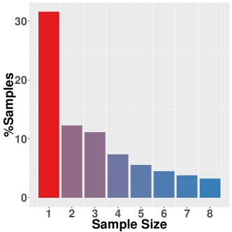
(a) Weighted Cascade (WC)

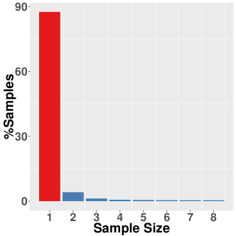
(b) Trivalency (TRI)

Figure 1: Distribution of reversed cascade sizes on Epinions network (and on other networks as well) with two different edge weight models: Weighted Cascade (WC) and Trivalency (TRI). The majority of the cascades are singular.

Common Shortcomings. According to recent benchmarks [10] and our own empirical evaluations (details in Section VII), both RIS and SKIM yield significant influence estimation errors. For RIS, it is due to the fact that the majority of RIS samples contain only their sources as demonstrated in Figure 1 with up to 86% of such RIS samples overall. These samples, termed singular, harm the performance in two ways: 1) they do not contribute to the influence computation of other seed sets than the ones that contain the sources, however, the contribution is known in advance, i.e. number of seed nodes; 2) these samples magnify the variance of the RIS-based random variables used in estimation causing high errors.

This motivates our Importance Sketching techniques to generate only non-singular samples that are useful for influence estimations of many seed sets (not just ones with the sources).

III Importance Sketching

This section introduces our core construction of Importance Sketching algorithm to generate random non-singular samples with probabilities proportional to those in the original sample space of reverse influence samples and normalized by the probability of generating a non-singular ones.

Input: Graph $\mathcal{G}=(V,E,w)$

Output: $R_{j}$ - A random IIS sample

1 Pick a node $v\in V$ as the source with probability in Eq. 8;

2 Select an in-neighbor $u_{i}$ of $v$, $u_{i}\in N^{in}(v)$, with probability of selecting $u_{i}$ given in Eq. 9;

3 Initialize a queue $Q=\{u_{i}\}$ and a node set $R_{j}=\{v,u_{i}\}$;

4 foreach $u_{t}\in N^{in}(v),t\neq i$ do

5       With probability $w(u_{t},v)$:

6         $Q.\textsf{push}(u_{t});R_{j}\leftarrow R_{j}\cup\{u_{t}\};$

7while $Q$ is not empty do

       $v=Q.\textsf{pop}()$;// get the longest inserted node

8       foreach $u\in N^{in}(v)\backslash(R_{j}\cup Q)$ do

9             With probability $w(u,v)$:

               $Q.\textsf{push}(u);R_{j}\leftarrow R_{j}\cup\{u\}$; // insert $u$

10            

11      

return $R_{j}$;

Algorithm 1 Importance Influence Sampling (IIS) Alg.

III-A Importance Influence Sampling (IIS)

Sample Spaces and Desired Property. Let $\Omega_{\textsf{RIS}}$ be the sampling space of reverse influence samples (RIS) with probability $\Pr[R_{j}\in\Omega_{\textsf{RIS}}]$ of generating sample $R_{j}$. Let $\Omega_{\textsf{SKIS}}$ be a subspace of $\Omega_{\textsf{RIS}}$ and corresponds to the space of only non-singular reverse influence samples in $\Omega_{\textsf{RIS}}$. Since $\Omega_{\textsf{SKIS}}$ is a subspace of $\Omega_{\textsf{RIS}}$, the probability $\Pr[R_{j}\in\Omega_{\textsf{SKIS}}]$ of generating a non-singular sample from $\Omega_{\textsf{SKIS}}$ is larger than that from $\Omega_{\textsf{RIS}}$. Specifically, for a node $v\in V$, let $\gamma_{v}$ be the probability of generating a non-singular sample if $v$ is selected as the source and $\Gamma=\sum_{v\in V}\gamma_{v}$. Then, since the sample sources are selected randomly, the ratio of generating a non-singular sample to generating any sample in $\Omega_{\textsf{RIS}}$ is $\frac{\Gamma}{n}$ and thus, the probability $\Pr[R_{j}\in\Omega_{\textsf{SKIS}}]$ is as follows,

$$\Pr[R_{j}\in\Omega_{\textsf{SKIS}}]=\frac{n}{\Gamma}\Pr[R_{j}\in\Omega_{\textsf{RIS}}].$$ (6)

Our upcoming IIS algorithm aims to achieve this desired property of sampling non-singular samples from $\Omega_{\textsf{SKIS}}$.

Sampling Algorithm. Our Importance Influence Sampling (IIS) scheme involves three core components:

• Probability of having a non-singular sample. For a node $v\in V$, a sample with source $v$ is singular if no in-neighbor of $v$ is selected, that happens with probability $\Pi_{u\in N^{in}(v)}(1-w(u,v))$. Hence, the probability of having a non-singular sample from a node $v$ is the complement:

  $$\gamma_{v}=1-\Pi_{u\in N^{in}(v)}(1-w(u,v)).$$ (7)

• Source Sampling Rate. Note that the set of non-singular samples is just a subset of all possible samples and we want to generate uniformly random samples from that subset. Moreover, each node $v$ has a probability $\gamma_{v}$ of generating a non-singular sample from it. Thus, in order to generate a random sample, we select $v$ as the source with probability $\Pr[\textsf{src}(R_{j})=v]$ computed as follows,

  $$\Pr[\textsf{src}(R_{j})=v]=\frac{\gamma_{v}}{\sum_{u\in V}\gamma_{u}}=\frac{\gamma_{v}}{\Gamma},$$ (8)

  where $\Gamma=\sum_{u\in V}\gamma_{u}$, and then generate a uniformly random non-singular sample from the specific source $v$ as described in the next component.

• Sample a non-singular sample from a source. From the $\textsf{src}(R_{j})=v$, we generate a non-singular sample $R_{j}$ from $v$ uniformly at random. Let $N^{in}(v)=\{u_{1},u_{2},\dots,u_{l}\}$ be a fixed-order set of in-neighbors of $v$. We divide the all possible non-singular samples from $v$ into $l$ buckets: bucket $B_{i},1\leq i\leq l$ contains those samples that have the first node from $N^{in}(v)$ being $u_{i}$. That means all the nodes $u_{1},\dots,u_{i-1}$ are not in the sample but $u_{i}$ is in for certain. The other nodes from $u_{i+1}$ to $u_{l}$ may appear and will be sampled following the normal RIS sampling. Now we select the bucket that $R_{j}$ belongs to with the probability of selecting $B_{i}$ being as follows,

  $$\Pr[\text{select }B_{i}]=\frac{\prod_{t=1}^{i-1}(1-w(u_{t},v))w(u_{i},v)}{\gamma_{v}}.$$ (9)

  For $i=1$, we have $\Pr[\text{select }B_{1}]=w(u_{1},v)$. Note that $\sum_{i=1}^{l}\Pr[\text{select }B_{i}]=1$. Assume bucket $B_{i}$ is selected and, thus, node $u_{i}$ is added as the second node besides the source into $R_{j}$. For each other node $u_{t},t\neq i$, $u_{t}$ is selected into $R_{j}$ with probability $w(u_{t},v)$ following the ordinary RIS for the IC model.

These three components guarantee a non-singular sample. The detailed description of IIS sampling is in Alg. 1. The first step selects the source of the IIS sample among $V$. Then, the first incoming node to the source $v$ is picked (Line 2) following the above description of the component 3). Each of the other incoming neighbors also tries to influence the source (Lines 4-6). The rest performs similarly as in RIS [5]. That is for each newly selected node, its incoming neighbors are randomly added into the sample with probabilities equal to their edge weights. It continues until no newly selected node is observed. Note that Line 3 only adds the selected neighbors $u_{i}$ of $v$ into $Q$ but adds both $v$ and $u_{i}$ to $R_{j}$. The loop from Lines 7-11 mimics the BFS-like sampling procedure of RIS.

Let $\Pr[R_{j}]$ be the probability of generating a non-singular sample $R_{j}$ using IIS algorithm. We have

$$\Pr[R_{j}] =\sum_{v\in V}\Pr[\textsf{src}(R_{j})=v]\Pr[\text{generate }R_{j}\text{ from }v]$$

$$=\sum_{v\in V}\frac{\gamma_{v}}{\Gamma}\frac{\Pr[R_{j}\in\Omega_{\textsf{RIS}}\text{ and }\textsf{src}(R_{j})=v]}{\gamma_{v}}$$

$$=\frac{n}{\Gamma}\sum_{v\in V}\frac{1}{n}\Pr[R_{j}\in\Omega_{\textsf{RIS}}\text{ and }\textsf{src}(R_{j})=v]$$

$$=\frac{n}{\Gamma}\Pr[R_{j}\in\Omega_{\textsf{RIS}}]=\Pr[R_{j}\in\Omega_{\textsf{SKIS}}],$$

where $\Pr[\text{generate }R_{j}\text{ from }v]=\frac{\Pr[R_{j}\in\Omega_{\textsf{RIS}}\text{ and }\textsf{src}(R_{j})=v]}{\gamma_{v}}$ due to the selection of the bucket that $R_{j}$ belongs to in IIS. Thus, the output $R_{j}$ of IIS is an random sample from non-singular space $\Omega_{\textsf{SKIS}}$ and we obtain the following lemma.

Lemma 2.

Recall that $\Omega_{\textsf{SKIS}{}}$ is the sample space of non-singular reverse influence samples. IIS algorithm generates a random non-singular sample from sample space $\Omega_{\textsf{SKIS}{}}$.

Connection between IIS Samples and Influences. We establish the following key lemma that connects our IIS samples with the influence of any seed set $S$.

Lemma 3.

Given a random IIS sample $R_{j}$ generated by Alg. 1 from the graph $\mathcal{G}=(V,E,w)$, for any set $S\subseteq V$, we have,

$$\mathbb{I}(S)=\Pr[R_{j}\cap S\neq\emptyset]\cdot\Gamma+\sum_{v\in S}(1-\gamma_{v}),$$ (10)

where $\gamma_{v}$ and $\Gamma$ are defined in Eqs. 7 and 8.

The proof is presented in our extended version [18]. The influence $\mathbb{I}(S)$ of any set $S$ comprises of two parts: 1) $\Pr[R_{j}\cap S\neq\emptyset]\cdot\Gamma$ depends on the randomness of $R_{j}$ and 2) the fixed amount $\sum_{v\in S}(1-\gamma_{v})$ that is inherent to set $S$ and accounts for the contribution of singular samples in $\Omega_{\textsf{RIS}}$ to the influence $\mathbb{I}(S)$. Lemma 3 states that instead of computing or estimating the influence $\mathbb{I}(S)$ directly, we can equivalently compute or estimate $\Pr[R_{j}\cap S\neq\emptyset]\cdot\Gamma+\sum_{v\in S}(1-\gamma_{v})$ using IIS samples.

Remark: Notice that we can further generate samples of larger sizes and reduce the variance as shown later, however, the computation would increase significantly.

IV Influence Oracle via IIS Sketch (SKIS)

We use IIS sampling to generate a sketch for answering influence estimation queries of different node sets. We show that the random variables associated with our samples have much smaller variances than that of RIS, and hence, lead to better concentration or faster estimation with much fewer samples required to achieve the same or better quality.

SKIS-based Influence Oracle. An SKIS sketch $\mathcal{R}$ is a collection of IIS samples generated by Alg. 1, i.e. $\mathcal{R}=\{R_{1},\dots,R_{T}\}$. As shown in Lemma 3, the influence $\mathbb{I}(S)$ can be estimated through estimating the probability $\Pr[R_{j}\cap S\neq\emptyset]$. Thus, from a SKIS sketch $\mathcal{R}=\{R_{1},\dots,R_{T}\}$, we can obtain an estimate $\hat{\mathbb{I}}(S)$ of $\mathbb{I}(S)$ for any set $S$ by,

$$\hat{\mathbb{I}}_{\mathcal{R}}(S)=\frac{\mathrm{C}_{\mathcal{R}}(S)}{|\mathcal{R}|}\cdot\Gamma+\sum_{v\in S}(1-\gamma_{v}),$$ (11)

where $\mathrm{C}_{\mathcal{R}}(S)$ is coverage of $S$ on $\mathcal{R}$, i.e.,

$$\mathrm{C}_{\mathcal{R}}(S)=|\{R_{j}\in\mathcal{R}|R_{j}\cap S\neq\emptyset\}|.$$ (12)

Input: Graph $\mathcal{G}=(V,E,w)$

1 Preprocessing: Generate a SKIS sketch $\mathcal{R}=\{R_{1},\dots,R_{T}\}$ of IIS samples using Alg. 1.

For any influence query for any set $S$: return $\hat{\mathbb{I}}_{\mathcal{R}}(S)$ (Eq. 11).

Algorithm 2 SKIS-based Influence Oracle

We build an SKIS-based oracle for influence queries by generating a set $\mathcal{R}$ of $T$ IIS samples in a preprocessing step and then answer influence estimation query $\hat{\mathbb{I}}_{\mathcal{R}}(S)$ for any requested set $S$ (Alg. 2). In the following, we show the better estimation quality of our sketch through analyzing the variances and estimating concentration properties.

SKIS Random Variables for Estimations. For a random IIS sample $R_{j}$ and a set $S$, we define random variables:

$$X_{j}(S)=\left\{\begin{array}[]{ll}1&\mbox{if }R_{j}\cap S\neq\emptyset\\ 0&\mbox{otherwise.}\end{array}\right.,\text{and}$$ (15)

$$Z_{j}(S)=\frac{X_{j}(S)\cdot\Gamma+\sum_{v\in S}(1-\gamma_{v})}{n}.$$ (16)

Then, the means of $X_{j}(S)$ and $Z_{j}(S)$ are as follows,

$$\mathbb{E}[X_{j}(S)]=\Pr[R_{j}\cap S\neq\emptyset]=\frac{\mathbb{I}(S)-\sum_{v\in S}(1-\gamma_{v})}{\Gamma}$$ (17)

$$\mathbb{E}[Z_{j}(S)]=\mathbb{E}[X_{j}(S)]\cdot\frac{\Gamma}{n}+\frac{\sum_{v\in S}(1-\gamma_{v})}{n}=\frac{\mathbb{I}(S)}{n}.$$ (18)

Hence, we can construct a corresponding set of random variables $Z_{1}(S),Z_{2}(S),\dots,Z_{T}(S)$ by Eqs. 15 and 16. Then, $\hat{\mathbb{I}}_{\mathcal{R}}(S)=\frac{n}{T}\sum_{j=1}^{T}Z_{j}(S)$ is an empirical estimate of $\mathbb{I}(S)$ based on the SKIS sketch $\mathcal{R}$.

For comparison purposes, let $Y_{j}(S)$ be the random variable associated with RIS sample $Q_{j}$ in a RIS sketch $\mathcal{Q}$,

$$Y_{j}(S)=\left\{\begin{array}[]{ll}1&\mbox{if }Q_{j}\cap S\neq\emptyset\\ 0&\mbox{otherwise.}\end{array}\right.$$ (21)

From Lemma 1, the mean value of $Y_{j}(S)$ is then,

$$\mathbb{E}[Y_{j}(S)]=\frac{\mathbb{I}(S)}{n}.$$ (22)

Variance Reduction Analysis. We show that the variance of $Z_{j}(S)$ for SKIS is much smaller than that of $Y_{j}(S)$ for RIS. The variance of $Z_{j}(S)$ is stated in the following.

Lemma 4.

The random variable $Z_{j}(S)$ (Eq. 16) has

$$\mathrm{Var} [Z_{j}(S)]=\frac{\mathbb{I}(S)}{n}\frac{\Gamma}{n}-\frac{\mathbb{I}^{2}(S)}{n^{2}}$$

$$-\frac{\sum_{v\in S}(1-\gamma_{v})}{n^{2}}(\Gamma+\sum_{v\in S}(1-\gamma_{v})-2\mathbb{I}(S)).$$ (23)

Since the random variables $Y_{j}(S)$ for RIS samples are Bernoulli and $\mathbb{E}[Y_{j}(S)]=\frac{\mathbb{I}(S)}{n}$, we have $\mathrm{Var}[Y_{j}(S)]=\frac{\mathbb{I}(S)}{n}(1-\frac{\mathbb{I}(S)}{n})$. Compared with $\mathrm{Var}[Z_{j}(S)]$, we observe that since $\frac{\Gamma}{n}\leq 1$, $\frac{\mathbb{I}(S)}{n}\frac{\Gamma}{n}-\frac{\mathbb{I}^{2}(S)}{n^{2}}\leq\frac{\mathbb{I}(S)}{n}-\frac{\mathbb{I}^{2}(S)}{n^{2}}=\mathrm{Var}[Y_{j}(S)]$,

$$\mathrm{Var}[Z_{j}(S)] \leq\mathrm{Var}[Y_{j}(S)]$$

$$-\frac{\sum_{v\in S}(1-\gamma_{v})}{n^{2}}(\Gamma+\sum_{v\in S}(1-\gamma_{v})-2\mathbb{I}(S)).$$

In practice, most of seed sets have small influences, i.e. $\mathbb{I}(S)\ll\frac{\Gamma}{2}$, thus, $\Gamma+\sum_{v\in S}(1-\gamma_{v})-2\mathbb{I}(S)\gg 0$. Hence, $\mathrm{Var}[Z_{j}(S)]<\mathrm{Var}[Y_{j}(S)]$ holds for most seed sets $S$.

Better Concentrations of SKIS Random Variables. Observe that $Z_{j}(S)\in\Big{[}\frac{\sum_{v\in S}(1-\gamma_{v})}{n},\frac{\Gamma+\sum_{v\in S}(1-\gamma_{v})}{n}\Big{]}$, we obtain another result on the variance of $Z_{j}(S)$ as follows.

Lemma 5.

The variance of random variable $Z_{j}(S)$ satisfies

$$\mathrm{Var}[Z_{j}(S)]\leq\frac{\mathbb{I}(S)}{n}\frac{\Gamma}{n}.$$ (24)

Using the above result with the general form of Chernoff’s bound in Lemma 2 in [7], we derive the following concentration inequalities for random variables $Z_{j}(S)$ of SKIS.

Lemma 6.

Given a SKIS sketch $\mathcal{R}=\{R_{1},\dots,R_{T}\}$ with random variables $Z_{1}(S),\dots,Z_{T}(S)$, we have,

$$\Pr\Big{[}\frac{\sum_{j=1}^{T}Z_{j}(S)}{T}n-\mathbb{I}(S)\geq\epsilon\mathbb{I}(S)\Big{]}\leq\exp\Big{(}\frac{-\epsilon^{2}T}{2\bm{\frac{\Gamma}{n}}+\frac{2}{3}\epsilon}\frac{\mathbb{I}(S)}{n}\Big{)}$$

$$\Pr\Big{[}\frac{\sum_{j=1}^{T}Z_{j}(S)}{T}n-\mathbb{I}(S)\leq-\epsilon\mathbb{I}(S)\Big{]}\leq\exp\Big{(}\frac{-\epsilon^{2}T}{2\bm{\frac{\Gamma}{n}}}\frac{\mathbb{I}(S)}{n}\Big{)}.$$

Compared with the bounds for RIS sketch in Corollaries 1 and 2 in [7], the above concentration bounds for SKIS sketch (Lemma 6) are stronger, i.e. tighter. Specifically, we have the factor $\frac{\Gamma}{n}$ in the denominator of the $\exp(.)$ function while for RIS random variables, it is simply $1$.

Sufficient Size of SKIS Sketch for High-quality Estimations. There are multiple strategies to determine the number of IIS samples generated in the preprocessing step. For example, [3] generates samples until total size of all samples reaches $O(\frac{1}{\epsilon^{3}}(n+m)\log(n))$. Generating IIS samples to reach such a specified threshold is vastly faster than using RIS due to the bigger size of IIS samples. This method provides an additive estimation error guarantee within $\epsilon$. Alternatively, by Lemma 6, we derive the sufficient number of IIS samples to provide the more preferable $(\epsilon,\delta)$-estimation of $\mathbb{I}(S)$.

Lemma 7.

Given a set $S$, $\epsilon,\delta\geq 0$, if the SKIS sketch $\mathcal{R}$ has at least $(2\frac{\Gamma}{n}+\frac{2}{3}\epsilon)\ln(\frac{2}{\delta})\frac{n}{\mathbb{I}(S)}\epsilon^{-2}$ IIS samples, $\hat{\mathbb{I}}_{\mathcal{R}}(S)$ is an $(\epsilon,\delta)$-estimate of $\mathbb{I}(S)$, i.e.,

$$\Pr[(1-\epsilon)\mathbb{I}(S)\leq\hat{\mathbb{I}}_{\mathcal{R}}(S)\leq(1+\epsilon)\mathbb{I}(S)]\geq 1-\delta.$$ (25)

In practice, $\mathbb{I}(S)$ is unknown in advance and a lower-bound of $\mathbb{I}(S)$, e.g. $|S|$, can be used to compute the necessary number of samples to provide the same guarantee. Compared to RIS with weaker concentration bounds, we save a factor of $O(\frac{\Gamma}{n})$.

V SKIS-based IM Algorithms

With the help of SKIS sketch that is better in estimating the influences compared to the well-known successful RIS, we can largely improve the efficiency of IM algorithms in the broad class of RIS-based methods, i.e. RIS [5], TIM/TIM+ [6], IMM [7], BCT [19, 20], SSA/DSSA [8]. This improvement is possible since these methods heavily rely on the concentration of influence estimations provided by RIS samples.

SKIS-based framework. Let $\mathcal{R}=\{R_{1},R_{2},\dots\}$ be a SKIS sketch of IIS samples. $\mathcal{R}$ gives an influence estimate

$$\hat{\mathbb{I}}_{\mathcal{R}}(S)=\hat{\mathbb{E}}_{\mathcal{R}}[Z_{j}(S)]\cdot n=\frac{\mathrm{C}_{\mathcal{R}}(S)}{|\mathcal{R}|}\cdot\Gamma+\sum_{v\in S}(1-\gamma_{v}),$$ (26)

for any set $S$. Thus, instead of optimizing over the exact influence, we can intuitively find the set $S$ to maximize the estimate function $\hat{\mathbb{I}}(S)$. Then, the framework of using SKIS sketch to solve IM problem contains two main steps:

• Generate a SKIS sketch $\mathcal{R}$ of IIS samples,

• Find the set $S_{k}$ that maximizes the function $\hat{\mathbb{I}}_{R}(S)$ and returning $S_{k}$ as the solution for the IM instance.

There are two essential questions related to the above SKIS-based framework : 1) Given a SKIS sketch $\mathcal{R}$ of IIS samples, how to find $S_{k}$ of $k$ nodes that maximizes $\hat{\mathbb{I}}_{\mathcal{R}}(S_{k})$ (in Step 2)? 2) How many IIS samples in the SKIS sketch $\mathcal{R}$ (in Step 1) are sufficient to guarantee a high-quality solution for IM?

We give the answers for the above questions in the following sections. Firstly, we adapt the gold-standard greedy algorithm to obtain an $(1-(1-1/k)^{k})$-approximate solution over a SKIS sketch. Secondly, we adopt recent techniques on RIS with strong solution guarantees to SKIS sketch.

Input: SKIS sketch $\mathcal{R}$ and $k$

Output: An $(1-(1-1/k)^{k})$-approximate seed set $\hat{S}_{k}$

1 $\hat{S}_{k}=\emptyset$

2 for $i=1:k$ do

3       $\hat{v}\leftarrow\arg\max_{v\in V\backslash\hat{S}_{k}}\big{(}\frac{\Delta_{\mathcal{R}}(v,\hat{S}_{k})}{|\mathcal{R}|}\Gamma+(1-\gamma_{v})\big{)}$

4       Add $\hat{v}$ to $\hat{S}_{k}$

5      

return $\hat{S}_{k}$

Algorithm 3 Greedy Algorithm on SKIS sketch

V-A Greedy Algorithm on SKIS Sketches

Let consider the optimization problem of finding a set $S_{k}$ of at most $k$ nodes to maximize the function $\hat{\mathbb{I}}_{\mathcal{R}}(S)$ on a SKIS sketch $\mathcal{R}$ of IIS samples under the cardinality constraint $|S|\leq k$. The function $\hat{\mathbb{I}}_{\mathcal{R}}(S)$ is monotone and submodular since it is the weighted sum of a set coverage function $\mathrm{C}_{\mathcal{R}}(S)$ and a linear term $\sum_{v\in S}(1-\gamma_{v})$. Thus, we obtain the following lemma with the detailed proof in our extended version [18].

Lemma 8.

Given a set of IIS samples $\mathcal{R}$, the set function $\hat{\mathbb{I}}_{\mathcal{R}}(S)$ defined in Eq. 26 is monotone and submodular.

Thus, a standard greedy scheme [21], which iteratively selects a node with highest marginal gain, gives an $(1-(1-\frac{1}{k})^{k})$, that converges to $(1-1/e)$ asymptotically, approximate solution $\hat{S}_{k}$. The marginal gain of a node $v$ with respect to a set $S$ on SKIS sketch $\mathcal{R}$ is defined as follows,

$$\textsf{gain}_{\mathcal{R}}(v,S)=\frac{\Delta_{\mathcal{R}}(v,\hat{S}_{k})}{|\mathcal{R}|}\Gamma+(1-\gamma_{v}),$$ (27)

where $\Delta_{\mathcal{R}}(v,S)=\mathrm{C}_{\mathcal{R}}(S\cup\{v\})-\mathrm{C}_{\mathcal{R}}(S)$ is called the marginal coverage gain of $v$ w.r.t. $S$ on SKIS sketch $\mathcal{R}$.

Given a collection of IIS samples $\mathcal{R}$ and a budget $k$, the Greedy algorithm is presented in Alg. 3 with a main loop (Lines 2-4) of $k$ iterations. Each iteration picks a node $\hat{v}$ having largest marginal gain (Eq. 27) with respect to the current partial solution $\hat{S}_{k}$ and adds it to $\hat{S}_{k}$. The approximation guarantee of the Greedy algorithm (Alg. 3) is stated below.

Lemma 9.

The Greedy algorithm (Alg. 3) returns an $(1-(1-\frac{1}{k})^{k})$-approximate solution $\hat{S}_{k}$,

$$\hat{\mathbb{I}}_{\mathcal{R}}(\hat{S}_{k})\geq(1-(1-\frac{1}{k})^{k})\hat{\mathbb{I}}_{\mathcal{R}}(S^{*}_{\mathcal{R}}),$$ (28)

where $S_{\mathcal{R}}^{*}$ is the optimal cover set of size $k$ on sketch $\mathcal{R}$.

The lemma is derived directly from the $1-(1-\frac{1}{k})^{k}$ approximation factor of the ordinary greedy algorithm [21].

V-B Sufficient Size of SKIS Sketch for IM

Since the SKIS sketch offers a similar greedy algorithm with approximation ratio $(1-(1-1/k)^{k})$ to the traditional RIS, we can combine SKIS sketch with any RIS-based algorithm, e.g. RIS[5], TIM/TIM+[6], IMM[7], BCT[20], SSA/DSSA[8]. We discuss the adoptions of two most recent and scalable algorithms, i.e. IMM[7] and SSA/DSSA[8].

IMM+SKIS. Tang et al. [7] provide a theoretical threshold

$$\theta_{\textsf{RIS}}=O\Big{(}(\log{n\choose k}+\log\delta^{-1})\frac{n}{\textsf{OPT}_{k}}\epsilon^{-2}\Big{)}$$ (29)

on the number of RIS samples to guarantee an $(1-1/e-\epsilon)$-approximate solution for IM problem with probability $1-\delta$.

Replacing RIS with IIS samples to build a SKIS sketch enables us to use the better bounds in Lemma 6. By the approach of IMM in [7] with Lemma 6, we reduce the threshold of samples to provide the same quality to,

$$\theta_{\textsf{SKIS}{}}=O\Big{(}\frac{\Gamma+k}{n}\theta_{\textsf{RIS}}\Big{)}.$$ (30)

SSA/DSSA+SKIS. More recently, Nguyen et al. [8] propose SSA and DSSA algorithms which implement the Stop-and-Stare strategy of alternating between finding candidate solutions and checking the quality of those candidates at exponential points, i.e. $2^{t},t\geq 1$, to detect a satisfactory solution at the earliest time.

Combining SKIS with SSA or DSSA brings about multiple benefits in the checking step of SSA/DSSA. The benefits stem from the better concentration bounds which lead to better error estimations and smaller thresholds to terminate the algorithms. The details are in our extended version [18].

VI Extensions to other diffusion models

The key step in extending our techniques for other diffusion models is devising an importance sketching procedure for each model. Fortunately, following the same designing principle as IIS, we can devise importance sketching procedures for many other diffusion models. We demonstrate this through two other equally important and widely adopted diffusion models, i.e. Linear Threshold [4] and Continuous-time model [13].

Linear Threshold model [4]. This model imposes a constraint that the total weights of incoming edges into any node $v\in V$ is at most 1, i.e. $\sum_{u\in N^{in}(v)}w(u,v)\leq 1$. Every node has a random activation threshold $\lambda_{v}\in[0,1]$ and gets activated if the total edge weights from active in-neighbors exceeds $\lambda_{v}$, i.e. $\sum_{u\in N^{in}(v),u\text{ is active}}w(u,v)\geq\lambda_{v}$. A RIS sampling for LT model [20] selects a random node as the source and iteratively picks at most one in-neighbor of the last activated node with probability being the edge weights, $w(u,v)$.

The importance sketching algorithm for the LT model has the following components:

• Probability of having a non-singular sample:

  $$\gamma_{v}=\sum_{u\in N^{in}(v)}w(u,v)$$ (31)

• Source Sampling Rate:

  $$\Pr[\textsf{src}(R_{j})=v]=\frac{\gamma_{v}}{\sum_{v\in V}\gamma_{v}}$$ (32)

• Sample a non-singular sample from a source.: select exactly one in-neighbor $u$ of $\textsf{src}(R_{j})=v$ with probability $\frac{w(u,v)}{\gamma_{v}}$. The rest follows RIS sampling [19].

Continuous-time model [13]. Here we have a deadline parameter $T$ of the latest activation time and each edge $(u,v)$ is associated with a length distribution, represented by a density function $\mathcal{L}_{(u,v)}(t)$, of how long it takes $u$ to influence $v$. A node $u$ is influenced if the length of the shortest path from any active node at time $0$ is at most $T$. The RIS sampling for the Continuous-time model [7] picks a random node as the source and invokes the Dijkstra’s algorithm to select nodes into $\textsf{src}(R_{j})$. When the edge $(u,v)$ is first visited, the activation time is sampled following its length distribution $\mathcal{L}_{(u,v)}(t)$. From the length distribution, we can compute the probability $p(u,v,T)$ of an edge $(u,v)$ having activation time at most $T$

$$p(u,v,T)=\int_{t=0}^{T}\mathcal{L}_{(u,v)}(t)dt$$ (33)

The importance sketching procedure for the Continuous-time model has the following components:

• Probability of having a non-singular sample:

  $$\gamma_{v}=1-\prod_{u\in N^{in}(v)}(1-p(u,v,T))$$ (34)

• Source Sampling Rate:

  $$\Pr[\textsf{src}(R_{j})=v]=\frac{\gamma_{v}}{\sum_{v\in V}\gamma_{v}}$$ (35)

• Sample a non-singular sample from a source.: Use a bucket system on $p(u,v,T)$ similarly to IIS to select the first in-neighbor $u$. The activation time of $u$ follows the normalized density function $\frac{\mathcal{L}_{(u,v)}(t)}{\gamma_{v}}$. Subsequently, it continues by following RIS sampling [7].

VII Experiments

We demonstrate the advantages of our SKIS sketch through a comprehensive set of experiments on the key influence estimation and maximization problems. Due to space limit, we report the results under the IC model and partial results for the LT model. However, the implementations for all models will be released on our website to produce complete results.

VII-A Experimental Settings

TABLE II: Datasets’ Statistics

Dataset	#Nodes	#Edges	Avg. Degree
NetPHY	$37\cdot 10^{3}$	$181\cdot 10^{3}$	9.8
Epinions	$75\cdot 10^{3}$	$841\cdot 10^{3}$	22.4
DBLP	$655\cdot 10^{3}$	$2\cdot 10^{6}$	6.1
Orkut	$3\cdot 10^{6}$	$234\cdot 10^{6}$	78.0
Twitter [22]	$41.7\cdot 10^{6}$	$1.5\cdot 10^{9}$	70.5
Friendster	$65.6\cdot 10^{6}$	$3.6\cdot 10^{9}$	109.6

Datasets. We use 6 real-world datasets from [23, 22] with size ranging from tens of thousands to as large as 65.6 million nodes and 3.6 billion edges. Table II gives a summary.

Algorithms compared. On influence estimation, we compare our SKIS sketch with:

• RIS [5]: The well-known RIS sketch.

• SKIM [2]: Combined reachability sketch. We run SKIM with default parameters in [2] ($k=l=64$). SKIM is modified to read graph from files instead of internally computing the edge weights.

Following [3], we generate samples into SKIS and RIS until the total size of all the samples reaches $h\cdot n\log n$ where $h$ is a constant. Here, $h$ is chosen in the set $\{5,10\}$.

On influence maximization, we compare:

• PMC [24]: A Monte-Carlo simulation pruned method with no guarantees. It only works on the IC model.

• IMM [7]: RIS-based algorithm with quality guarantees.

• DSSA [8]: The current fastest RIS-based algorithm with approximation guarantee.

• DSSA+SKIS: A modified version of DSSA where SKIS sketch is adopted to replace RIS.

We set $\epsilon=0.5,\delta=1/n$ for the last three algorithms. For PMC, we use the default parameter of 200 DAGs.

Metrics. We compare the algorithms in terms of the solution quality, running time and memory usage. To compute the solution quality of a seed set, we adopt the relative difference which is defined as $\frac{|\hat{\mathbb{I}}(S)-\mathbb{I}(S)|}{\max\{\mathbb{I}(S),\hat{\mathbb{I}}(S)\}}\cdot 100\%$, where $\hat{\mathbb{I}}(S)$ is an estimate, and $\mathbb{I}(S)$ is the “ground-truth” influence of $S$.

Ground-truth Influence. Unlike previous studies [7, 2, 24] using a constant number of cascade simulations, i.e. 10000, to measure the ground-truth influence with unknown accuracy, we adopt the Monte-Carlo Stopping-Rule algorithm [25] that guarantees an estimation error less than $\epsilon$ with probability at least $1-\delta$ where $\epsilon=0.005,\delta=1/n$. Specifically, let $W_{j}$ be the size of a random influence cascade and $Z_{j}=\frac{W_{j}}{n}$ with $\mathbb{E}[Z_{j}]=\mathbb{I}(S)/n$ and $0\leq Z_{j}\leq 1$. The Monte-Carlo method generates sample $Z_{j}$ until $\sum_{j=1}^{T}Z_{j}\geq 4(e-2)\ln(\frac{2}{\delta})\frac{1}{\epsilon^{2}}$ and returns $\hat{\mathbb{I}}(S)=\frac{\sum_{j=1}^{T}Z_{j}}{T}n$ as the ground-truth influence.

For Twitter and Friendster dataset, we set $\epsilon=0.05$, and $\delta=1/n$ to compute ground-truth due to the huge computational cost in these networks. For the other networks, we keep the default setting of $\epsilon$ and $\delta$ as specified above.

Weight Settings. We consider two widely-used models:

• Weighted Cascade (WC) [6, 2, 7, 8]: The weight of edge $(u,v)$ is inversely proportional to the in-degree of node $v$, $d_{in}(v)$, i.e. $w(u,v)=\frac{1}{d_{in}(v)}$.

• Trivalency (TRI) [2, 26, 27]: The weight $w(u,v)$ is selected randomly from the set $\{0.1,0.01,0.001\}$.

Environment. We implemented our algorithms in C++ and obtained the implementations of others from the corresponding authors. We conducted all experiments on a CentOS machine with Intel Xeon E5-2650 v3 2.30GHz CPUs and 256GB RAM. We compute the ground-truth for our experiments in a period of 2 months on a cluster of 16 CentOS machines, each with 64 Intel Xeon CPUs X5650 2.67GHz and 256GB RAM.

TABLE III: Average relative differences (dnf: “did not finish” within 24h). SKIS almost always returns the lowest errors.

		WC Model								TRI Model
		SKIS			RIS			SKIM		SKIS			RIS			SKIM
$|S|$	Nets	$h(5)$	$h(10)$		$h(5)$	$h(10)$		$k(64)$		$h(5)$	$h(10)$		$h(5)$	$h(10)$		$k(64)$
l	PHY	6.2	3.7		14.0	7.8		7.5		1.7	1.3		11.8	8.2		4.5
	Epin.	4.7	3.0		15.7	11.8		19.6		16.6	14.2		55.3	47.4		27.7
	DBLP	3.8	4.1		13.7	11.6		5.0		0.9	0.7		9.4	6.4		3.5
	Orkut	10.3	9.2		13.5	8.8		77.6		9.3	9.9		14.5	10.8		dnf
	Twit.	10.9	10.5		21.4	16.0		29.1		81.4	81.9		80.8	81.5		dnf
	Frien.	15.9	10.2		22.2	13.3		dnf		29.8	21.3		28.5	23.6		dnf
$10^{2}$	PHY	0.9	0.6		1.0	0.7		2.1		0.3	0.2		1.1	0.9		1.8
	Epin.	1.0	0.7		1.0	1.0		7.6		0.2	1.5		4.4	1.8		2.8
	DBLP	0.9	0.6		1.9	1.4		5.0		0.8	0.7		5.5	5.3		5.5
	Orkut	0.9	0.6		1.1	0.7		56.5		0.1	0.2		4.2	0.9		dnf
	Twit.	1.1	1.2		1.3	1.1		60.2		4.3	3.1		6.4	5.5		dnf
	Frien.	0.9	0.7		0.9	0.7		dnf		1.9	1.9		0.6	2.0		dnf
$10^{3}$	PHY	0.6	0.8		0.9	1.0		0.6		0.3	0.4		1.2	1.3		1.1
	Epin.	0.6	0.6		0.6	0.7		2.3		2.3	0.3		1.9	4.6		1.5
	DBLP	0.2	0.3		0.2	0.2		1.7		0.1	0.0		0.3	0.2		0.3
	Orkut	0.3	0.3		0.3	0.3		50.7		2.5	1.1		6.8	2.1		dnf
	Twit.	0.9	0.9		1.0	0.9		36.3		0.9	2.4		4.1	2.8		dnf
	Frien.	0.3	0.3		0.3	0.2		dnf		1.9	1.9		0.6	2.0		dnf

TABLE IV: Sketch construction time and index memory of algorithms on different edge models. SKIS and RIS uses roughly the same time and memory and less than that of SKIM.

Index Time

Index Memory

[second (or h for hour)]

[MB (or G for GB)]

SKIS

RIS

SKIM

SKIS

RIS

SKIM

M

Nets

$h(5)$

$h(10)$

$h(5)$

$h(10)$

$k(64)$

$h(5)$

$h(10)$

$h(5)$

$h(10)$

$k(64)$

WC

PHY

0

1

1

1

2

41

83

52

105

105

Epin.

1

1

1

1

10

63

126

81

162

220

DBLP

10

18

7

14

37

702

1G

848

2G

2G

Orkut

92

157

69

148

0.6h

2G

5G

3G

5G

9G

Twit.

0.6h

0.9h

0.4h

1.0h

5.2h

38G

76G

42G

84G

44G

Frien.

0.8h

1.8h

0.8h

1.9h

dnf

59G

117G

61G

117G

dnf

TRI

PHY

0

1

1

2

1

46

90

97

194

99

Epin.

1

1

1

1

29

41

82

41

84

230

DBLP

11

34

18

36

22

1G

2G

2G

5G

2G

Orkut

88

206

89

197

dnf

2G

4G

2G

4G

dnf

Twit.

0.6h

1.2h

0.5h

1.3h

dnf

36G

69G

36G

69G

dnf

Frien.

0.9h

2.3h

1.0h

2.4h

dnf

54G

108G

54G

108G

dnf

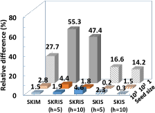
(a) TRI model

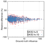
(b) SKIS-WC model

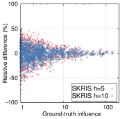
(c) RIS-WC model

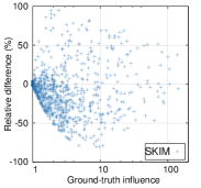
(d) SKIM-WC model

Figure 2: a) Relative difference on Epinions under TRI model and b), c), d) error distributions under WC model with $|S|=1$. SKIS has the lowest relative errors which highly concentrates around 0 while RIS’s and SKIM’s errors widely spread out.

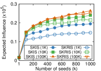
(a) Epinions

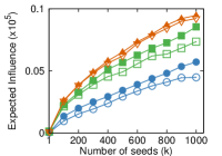
(b) NetPHY

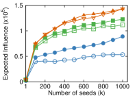
(c) DBLP

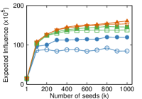
(d) Twitter

Figure 3: Efficiency of SKIS and RIS sketches in finding the maximum seed sets. SKIS sketch is up to 80% more efficient.

VII-B Influence Estimation

We show that SKIS sketch consumes much less time and memory space while consistently obtaining better solution quality, i.e. very small errors, than both RIS and SKIM.

VII-B1 Solution Quality

Table III and Figure 2 present the relative estimation errors of all three sketches.

The solution quality of SKIS is consistently better than RIS and SKIM across all the networks and edge models. As shown in Table III, the errors of SKIS are 110% and 400% smaller than those of RIS with $k=1$ while being as good as or better than RIS for $k=100,1000$. On the other hand, SKIM shows the largest estimation errors in most of the cases. Particularly, SKIM’s error is more than 60 times higher than SKIS and RIS on Twitter when $|S|=100$. Similar results are observed under TRI model. Exceptionally, on Twitter and Friendster, the relative difference of RIS is slightly smaller than SKIS with $h=5$ but larger on $h=10$. In TRI model, estimating a random seed on large network as Twitter produces higher errors since we have insufficient number of samples.

Figures 2b, c, and d draw the error distributions of sketches for estimating the influences of random seeds. Here, we generate 1000 uniformly random nodes and consider each node to be a seed set. We observe that SKIS’s errors are highly concentrated around 0% even when the influences are small while errors of RIS and SKIM spread out widely. RIS reveals extremely high errors for small influence estimation, e.g. up to $80\%$. The error distribution of SKIM is the most widely behaved, i.e. having high errors at every influence level. Under TRI model (Figure 2a), SKIS also consistently provides significantly smaller estimation errors than RIS and SKIM.

VII-B2 Performance

We report indexing time and memory of different sketches in Table IV.

Indexing Time. SKIS and RIS use roughly the same amount of time for build the sketches while SKIM is much slower than SKIS and RIS and failed to process large networks in both edge models. On larger networks, SKIS is slightly faster than RIS. SKIM markedly spends up to 5 hours to build sketch for Twitter on WC model while SKIS, or RIS spends only 1 hour or less on this network.

Index Memory. In terms of memory, the same observations are seen as with indexing time essentially because larger sketches require more time to construct. In all the experiments, SKIS consumes the same or less amount of memory with RIS. SKIM generally uses more memory than SKIS and RIS.

In summary, SKIS consistently achieves better solution quality than both RIS and SKIM on all the networks, edge models and seed set sizes while consuming the same or less time/memory. The errors of SKIS is highly concentrated around 0. In contrast, RIS is only good for estimating high influence while incurring significant errors for small ranges.

TABLE V: Performance of IM algorithms with $k=100$ (dnf: “did not finish” within 6h, mem: “out of memory”).

		Running Time [s (or h)]					Total Memory [M (or G)]					Expected Influence (%)					#Samples [$\times 10^{3}$]
	Nets	IMM	PMC	DSSA	DSSA		IMM	PMC	DSSA	DSSA		IMM	PMC	DSSA	DSSA		IMM	DSSA	DSSA
					+SKIS					+SKIS					+SKIS				+SKIS
WC	PHY	0.1	3.1	0.0	0.0		31	86	26	9		6.64	6.7	5.33	5.34		103.3	8.9	3.8
	Epin.	0.2	10.5	0.0	0.0		39	130	34	17		19.4	19.8	17.9	16.6		39.8	4.48	0.9
	DBLP	1.1	137.4	0.1	0.1		162	60	136	113		10.8	11.2	9.3	8.5		93.0	5.4	2.6
	Orkut	24.1	1.4h	2.6	0.9		4G	6G	2G	2G		6.7	8.7	5.7	5.1		174.4	11.52	2.6
	Twit.	67.3	mem	5.5	6.3		30G	mem	17G	16G		25.80	mem	24.1	21.0		54.0	18.0	0.8
	Frien.	dnf	mem	78.3	43.6		dnf	mem	35G	36G		dnf	mem	0.35	0.35		mem	215.0	102.4
TRI	PHY	0.2	1.5	0.0	0.0		50	61	30	9		1.77	1.73	1.4	1.5		370.1	35.8	3.8
	Epin.	13.9	6.9	2.0	0.6		483	40	72	33		5.7	5.9	5.47	5.46		123.0	8.9	0.5
	DBLP	3.2	20.1	0.3	0.2		389	54	191	118		0.32	0.31	0.28	0.24		3171.0	348.2	20.5
	Orkut	dnf	0.3h	1.3h	0.2h		dnf	16G	28G	11G		dnf	67.3	67.9	67.8		dnf	1.4	0.3
	Twit.	dnf	mem	5.2h	0.6h		dnf	mem	100G	28G		dnf	mem	24.2	24.4		dnf	3.4	0.4
	Frien.	dnf	mem	mem	3.1h		dnf	mem	mem	99G		dnf	mem	mem	40.1		dnf	mem	0.2

VII-C Influence Maximization

This subsection illustrates the advantage of IIS sketch in finding the seed set with maximum influence. The results show that IIS samples drastically speed up the computation time. DSSA+SKIS is the first to handle billion-scale networks on the challenging TRI edge model. We limit the running time for algorithms to 6 hours and put “dnf” if they cannot finish.

VII-C1 Identifiability of the Maximum Seed Sets

We compare the ability of the new IIS with the traditional RIS sampling in terms of identifying the seed set with maximum influence. We fix the number of samples generated to be in the set $\{1000,10000,100000\}$ and then apply the Greedy algorithm to find solutions. We recompute the influence of returned seed sets using Monte-Carlo method with precision parameters $\epsilon=0.005,\delta=1/n$. The results is presented in Figure 3.

From Figure 3, we observe a recurrent consistency that IIS samples return a better solution than RIS over all the networks, $k$ values and number of samples. Particularly, the solutions provided by IIS achieve up to $80\%$ better than those returned by RIS. When more samples are used, the gap gets smaller.

VII-C2 Efficiency of SKIS on IM problem

Table V presents the results of DSSA-SKIS, DSSA, IMM and PMC in terms of running time, memory consumption and samples generated.

Running Time. From Table V, the combination DSSA+SKIS outperforms the rest by significant margins on all datasets and edge models. DSSA-SKIS is up to 10x faster than the original DSSA. DSSA+SKIS is the first and only algorithm that can run on the largest network on TRI model.

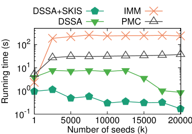
(a) Epinions

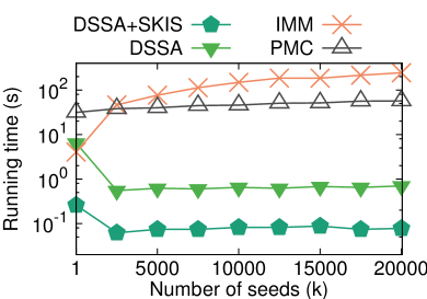
(b) DBLP

Figure 4: Running time of algorithms under the IC model.

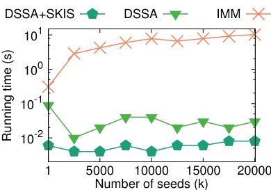
(a) Epinions

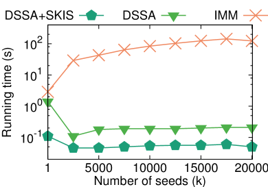
(b) DBLP

Figure 5: Running time of algorithms under the LT model.

Figure 4 compares the running time of all IM algorithms across a wide range of budget $k=1..20000$ under IC and TRI edge weight model. DSSA+SKIS always maintains significant performance gaps to the other algorithms, e.g. 10x faster than DSSA or 1000x faster than IMM and PMC.

Number of Samples and Memory Usage. On the same line with the running time, the memory usage and number of samples generated by DSSA+SKIS are much less than those required by the other algorithms. The number of samples generated by DSSA+SKIS is up to more 10x smaller than DSSA on TRI model, 100x less than IMM. Since the memory for storing the graph is counted into the total memory, the memory saved by DSSA+SKIS is only several times smaller than those of DSSA and IMM. PMC exceptionally requires huge memory and is unable to run on two large networks.

Experiments on the Linear Threshold (LT) model. We carry another set of experiments on the LT model with multiple budget $k$. Since in LT, the total weights of incoming edge to every node are bounded by 1, for each node, we first normalized the weights of incoming edges and then multiply them with a random number uniformly generated in $[0,1]$.

The results are illustrated in Figure 5. Similar observations to the IC are seen in the LT model that DSSA+SKIS runs faster than the others by orders of magnitude.

Overall, DSSA+SKIS reveals significant improvements over the state-of-the-art algorithms on influence maximization. As a result, DSSA+SKIS is the only algorithm that can handle the largest networks under different models.

VIII Conclusion

We propose SKIS - a novel sketching tools to approximate influence dynamics in the networks. We provide both comprehensive theoretical and empirical analysis to demonstrate the superiority in size-quality trade-off of SKIS in comparisons to the existing sketches. The application of SKIS to existing algorithms on Influence Maximization leads to significant performance boost and easily scale to billion-scale networks. In future, we plan to extend SKIS to other settings including evolving networks and time-based influence dynamics.

-A Proof of Lemma 3

Given a stochastic graph $\mathcal{G}$, recall that $\Omega_{\mathcal{G}}$ is the space of all possible sample graphs $g\sim\mathcal{G}$ and $\Pr[g]$ is the probability that $g$ is realized from $\mathcal{G}$. In a sample graph $g\in\Omega_{\mathcal{G}}$, $\eta_{g}(S,v)=1$ if $v$ is reachable from $S$ in $g$. Consider the graph sample space $\Omega_{\mathcal{G}}$, based on a node $v\in V\backslash S$, we can divide $\Omega_{\mathcal{G}}$ into two partitions: 1) $\Omega^{\emptyset}_{\mathcal{G}}(v)$ contains those samples $g$ in which $v$ has no incoming live-edges; and 2) $\bar{\Omega}^{\emptyset}_{\mathcal{G}}(v)=\Omega_{\mathcal{G}}\backslash\Omega^{\emptyset}_{\mathcal{G}}$. We start from the definition of influence spread as follows,

$$\mathbb{I}(S) =\sum_{v\in V}\sum_{g\in\Omega_{\mathcal{G}}}\eta_{g}(S,v)\Pr[g]$$

$$=\sum_{v\in V}\Big{(}\sum_{g\in\Omega^{\emptyset}_{\mathcal{G}}(v)}\eta_{g}(S,v)\Pr[g]+\sum_{g\in\bar{\Omega}^{\emptyset}_{\mathcal{G}}(v)}\eta_{g}(S,v)\Pr[g]\Big{)}.$$

In each $g\in\Omega^{\emptyset}_{\mathcal{G}}(v)$, the node $v$ does not have any incoming nodes, thus, $\eta_{g}(S,v)=1$ only if $v\in S$. Thus, we have that $\sum_{v\in V}\sum_{g\in\Omega^{\emptyset}_{\mathcal{G}}(v)}\eta_{g}(S,v)\Pr[g]=\sum_{v\in S}\sum_{g\in\Omega^{\emptyset}_{\mathcal{G}}(v)}\Pr[g]$. Furthermore, the probability of a sample graph which has no incoming live-edge to $v$ is $\sum_{g\in\Omega^{\emptyset}_{\mathcal{G}}(v)}\Pr[g]=1-\gamma_{v}$. Combine with the above equiation of $\mathbb{I}(S)$, we obtain,

$$\mathbb{I}(S)=\sum_{v\in S}(1-\gamma_{v})+\sum_{v\in V}\sum_{g\in\bar{\Omega}^{\emptyset}_{\mathcal{G}}(v)}\eta_{g}(S,v)\Pr[g\in\Omega_{\mathcal{G}}].$$ (36)

Since our IIS sketching algorithm only generates samples corresponding to sample graphs from the set $\bar{\Omega}^{\emptyset}_{\mathcal{G}}(v)$, we define $\bar{\Omega}^{\emptyset}_{\mathcal{G}}(v)$ to be a graph sample space in which the sample graph $\bar{g}\in\bar{\Omega}^{\emptyset}_{\mathcal{G}}(v)$ has a probability $\Pr[\bar{g}\in\bar{\Omega}^{\emptyset}_{\mathcal{G}}(v)]=\frac{\Pr[\bar{g}\in\Omega_{\mathcal{G}}]}{\gamma_{v}}$ of being realized (since $\sum_{\bar{g}\in\bar{\Omega}^{\emptyset}_{\mathcal{G}}(v)}\Pr[\bar{g}\in\Omega_{\mathcal{G}}]=\gamma_{v}$ is the normalizing factor to fulfill a probability distribution of a sample space). Then, Eq. 36 is rewritten as follows,

$$\mathbb{I}(S) =\sum_{v\in V}\sum_{g\in\bar{\Omega}^{\emptyset}_{\mathcal{G}}(v)}\eta_{g}(S,v)\frac{\Pr[g\in\Omega_{\mathcal{G}}]}{\gamma_{v}}\gamma_{v}+\sum_{v\in S}(1-\gamma_{v})$$

$$=\sum_{v\in V}\sum_{\bar{g}\in\bar{\Omega}^{\emptyset}_{\mathcal{G}}(v)}\eta_{\bar{g}}(S,v)\Pr[\bar{g}\in\bar{\Omega}^{\emptyset}_{\mathcal{G}}(v)]\gamma_{v}+\sum_{v\in S}(1-\gamma_{v})$$

Now, from the node $v$ in a sample graph $\bar{g}\in\bar{\Omega}^{\emptyset}_{\mathcal{G}}(v)$, we have a IIS sketch $R_{j}(\bar{g},v)$ starting from $v$ and containing all the nodes that can reach $v$ in $\bar{g}$. Thus, $\eta_{\bar{g}}(S,v)=\textbf{1}_{R_{j}(\bar{g},v)\cap S\neq\emptyset}$ where $\textbf{1}_{x}$ is an indicator function returning 1 iff $x\neq 0$. Then,

$$\sum_{\bar{g}\in\bar{\Omega}^{\emptyset}_{\mathcal{G}}(v)}\eta_{\bar{g}}(S,v)\Pr[\bar{g}\in\bar{\Omega}^{\emptyset}_{\mathcal{G}}(v)]$$

$$=\sum_{\bar{g}\in\bar{\Omega}^{\emptyset}_{\mathcal{G}}(v)}\textbf{1}_{R_{j}(\bar{g},v)\cap S\neq\emptyset}\Pr[\bar{g}\in\bar{\Omega}^{\emptyset}_{\mathcal{G}}(v)]=\Pr[R_{j}(v)\cap S\neq\emptyset]$$

where $R_{j}(v)$ is a random IIS sketch with $\textsf{src}(R_{j}(v))=v$. Plugging this back into the computation of $\mathbb{I}(S)$ gives,

$$\mathbb{I}(S)=\sum_{v\in V}\Pr[R_{j}(v)\cap S\neq\emptyset]\gamma_{v}+\sum_{v\in S}(1-\gamma_{v})$$

$$=\sum_{v\in V}\Pr[R_{j}(v)\cap S\neq\emptyset]\frac{\gamma_{v}}{\Gamma}\Gamma+\sum_{v\in S}(1-\gamma_{v})$$

$$=\sum_{v\in V}\Pr[R_{j}(v)\cap S\neq\emptyset]\Pr[\textsf{src}(R_{j})=v]\Gamma+\sum_{v\in S}(1-\gamma_{v})$$

$$=\Pr[R_{j}\cap S\neq\emptyset]\cdot\Gamma+\sum_{v\in S}(1-\gamma_{v})$$ (37)

That completes the proof.

-B Proof of Lemma 4

From the basic properties of variance, we have,

$$\mathrm{Var}[Z_{j}(S)] =\mathrm{Var}[\frac{X_{j}(S)\cdot\Gamma+\sum_{v\in S}(1-\gamma_{v})}{n}]$$

$$=\frac{\Gamma^{2}}{n^{2}}\mathrm{Var}[X_{j}(S)]$$

Since $X_{j}(S)$ is a Bernoulli random variable with its mean value $\mathbb{E}[X_{j}(S)]=\frac{\mathbb{I}(S)-\sum_{v\in S}(1-\gamma_{v})}{\Gamma}$, the variance $\mathrm{Var}[X_{j}(S)]$ is computed as follows,

$$\mathrm{Var}[X_{j}(S)]$$

$$=\frac{\mathbb{I}(S)-\sum_{v\in S}(1-\gamma_{v})}{\Gamma}(1-\frac{\mathbb{I}(S)-\sum_{v\in S}(1-\gamma_{v})}{\Gamma})$$

$$=\frac{\mathbb{I}(S)}{\Gamma}-\frac{\mathbb{I}^{2}(S)}{\Gamma^{2}}-\frac{\sum_{v\in S}(1-\gamma_{v})}{\Gamma^{2}}(\Gamma+\sum_{v\in S}(1-\gamma_{v})-2\mathbb{I}(S))$$

Put this back into the variance of $Z_{j}(S)$ proves the lemma.

-C Proof of Lemma 5

Since $Z_{j}(S)$ takes values of either $\frac{\sum_{v\in S}(1-\gamma_{v})}{n}$ or $\frac{\Gamma+\sum_{v\in S}(1-\gamma_{v})}{n}$ and the mean value $\mathbb{E}[Z_{j}(S)]=\frac{\mathbb{I}(S)}{n}$, i.e. $\frac{\sum_{v\in S}(1-\gamma_{v})}{n}\leq\frac{\mathbb{I}(S)}{n}\leq\frac{\Gamma+\sum_{v\in S}(1-\gamma_{v})}{n}$. The variance of $Z_{j}(S)$ is computed as follows,

$$\mathrm{Var} [Z_{j}(S)]$$

$$=\Big{(}\frac{\mathbb{I}(S)}{n}-\frac{\sum_{v\in S}(1-\gamma_{v})}{n}\Big{)}\Big{(}\frac{\Gamma+\sum_{v\in S}(1-\gamma_{v})}{n}-\frac{\mathbb{I}(S)}{n}\Big{)}$$

$$\leq\frac{\mathbb{I}(S)}{n}\Big{(}\frac{\Gamma+\sum_{v\in S}(1-\gamma_{v})}{n}-\frac{\sum_{v\in S}(1-\gamma_{v})}{n}\Big{)}$$

$$=\frac{\mathbb{I}(S)}{n}\frac{\Gamma}{n}$$ (38)

-D Proof of Lemma 6

Lemma 2 in [7] states that:

Lemma 10.

Let $M_{1},M_{2},\dots$ be a martingale, such that $|M_{1}|\leq a$, $|M_{j}-M_{j-1}|\leq a$ for any $j\in[2,T]$, and

$$\mathrm{Var}[M_{1}]+\sum_{j=2}^{T}\mathrm{Var}[M_{j}|M_{1},M_{2},\dots,M_{j-1}]\leq b,$$ (39)

where $\mathrm{Var}[.]$ denotes the variances of a random variable. Then, for any $\lambda>0$,

$$\Pr[M_{T}-\mathbb{E}[M_{T}]\geq\lambda]\leq\exp\Big{(}-\frac{\lambda^{2}}{\frac{2}{3}a\lambda+2b}\Big{)}$$ (40)

Note that uniform random variables are also a special type of martingale and the above lemma holds for random variable as well. Let $p=\frac{\mathbb{I}(S)}{n}$. For RIS samples, since

• $|M_{1}|\leq 1$,

• $|M_{j}-M_{j-1}|\leq 1,\forall j\in[2,T]$,

• $\mathrm{Var}[M_{1}]+\sum_{j=2}^{T}\mathrm{Var}[M_{j}|M_{1},\dots,M_{j-1}]=\sum_{j=1}^{i}\mathrm{Var}[Y_{j}(S)]=Tp(1-p)\leq Tp$,

applying Eq. 40 for $\lambda=\epsilon Tp$ gives the following Chernoff’s bounds,

$$\Pr\Big{[}\sum_{j=1}^{T}X_{j}(S)-Tp\geq\epsilon Tp\Big{]}\leq\exp\Big{(}-\frac{\epsilon^{2}}{2+\frac{2}{3}\epsilon}Tp\Big{)},$$ (41)

and,

$$\Pr\Big{[}\sum_{j=1}^{T}X_{j}(S)-Tp\leq-\epsilon Tp\Big{]}\leq\exp\Big{(}-\frac{\epsilon^{2}}{2}Tp\Big{)}.$$ (42)

However, for IIS samples in SKIS sketch, the corresponding random variables $Z_{j}(S)$ replace $Y_{j}(S)$ and have the following properties:

• $|M_{1}|\leq\frac{\Gamma+\sum_{v\in S}(1-\gamma_{v})}{n}\leq 1$,

• $|M_{j}-M_{j-1}|\leq 1,\forall j\in[2,T]$,

• The sum of variances:

  $$\mathrm{Var}[M_{1}]+\sum_{j=2}^{T}\mathrm{Var}[M_{j}|M_{1},\dots,M_{j-1}]$$

  $$=\sum_{j=1}^{i}\mathrm{Var}[Z_{j}(S)]=Tp\frac{\Gamma}{n}$$ (43)

Thus, applying the general bound in Eq. 40 gives,

$$\Pr\Big{[}\sum_{j=1}^{T}X_{j}(S)-Tp\geq\epsilon Tp\Big{]}\leq\exp\Big{(}-\frac{\epsilon^{2}}{2\bm{\frac{\Gamma}{n}}+\frac{2}{3}\epsilon}Tp\Big{)},$$ (44)

and,

$$\Pr\Big{[}\sum_{j=1}^{T}X_{j}(S)-Tp\leq-\epsilon Tp\Big{]}\leq\exp\Big{(}-\frac{\epsilon^{2}}{2\bm{\frac{\Gamma}{n}}}Tp\Big{)}.$$ (45)

Note the factor $\frac{\Gamma}{n}$ is added in the denominator of the terms in the $\exp(.)$ function. Since $2\frac{\Gamma}{n}$ dominates $\frac{2}{3}\epsilon$, the concentration bounds for $Z_{j}(S)$ for SKIS are tighter than those of $Y_{j}(S)$ for RIS given in Eqs. 41 and 42.

-E Proof of Lemma 8

Since the function $\hat{\mathbb{I}}_{\mathcal{R}}(S)$ contains two additive terms, it is sufficient to show that each of them is monotone and submodular. The second term $\sum_{v\in S}(1-\gamma_{v})$ is a linear function and thus, it is monotone and submodular. For the first additive term, we see that $\frac{\Gamma}{|\mathcal{R}|\cdot n}$ is a constant and only need to show that $\mathrm{C}_{\mathcal{R}}(S)$ is monotone and submodular. Given the collection of IIS samples $\mathcal{R}$ in which $R_{j}\in\mathcal{R}$ is a list of nodes, the function $\mathrm{C}_{\mathcal{R}}(S)$ is just the count of IIS samples that intersect with the set $S$. In other words, it is equivalent to a covering function in a set system where IIS samples are elements and nodes are sets. A set covers an element if the corresponding node is contained in the corresponding IIS sample. It is well known that any covering function is monotone and submodular [28] and thus, the $\mathrm{C}_{\mathcal{R}}(S)$ has the same properties.

-F Improvements of SSA/DSSA using SKIS sketch

Recall that the original Stop-and-Stare strategy in [8] uses two independent sets of RIS samples, called $\mathcal{R}$ and $\mathcal{R}^{c}$. The greedy algorithm is applied on the first set $\mathcal{R}$ to find a candidate set $\hat{S}_{k}$ along with an estimate $\hat{\mathbb{I}}_{\mathcal{R}}(\hat{S}_{k})$ and the second set $\mathcal{R}^{c}$ is used to reestimate the influence of $\hat{S}_{k}$ by $\hat{\mathbb{I}}_{\mathcal{R}^{c}}(\hat{S}_{k})$. Now, SSA and DSSA have different ways to check the solution quality.

SSA. It assumes a set of fixed precision parameters $\epsilon_{1},\epsilon_{2},\epsilon_{3}$ such that $\frac{\epsilon_{1}+\epsilon_{2}+\epsilon_{1}\epsilon_{2}+\epsilon_{3}}{(1+\epsilon_{1})(1+\epsilon_{2})}(1-1/e)\leq\epsilon$. The algorithm stops when two conditions are met:

• $\mathrm{C}_{\mathcal{R}}(\hat{S}_{k})\geq\Lambda_{1}$ where $\Lambda_{1}=O(\log\frac{\delta}{t_{max}}\epsilon_{3}^{-2})$ and $t_{max}$ is a precomputed number depending on the size of the input graph $\mathcal{G}$.

• $\hat{\mathbb{I}}_{\mathcal{R}}(\hat{S}_{k})\leq(1+\epsilon_{1})\hat{\mathbb{I}}_{\mathcal{R}^{c}}(\hat{S}_{k})$.

$\Rightarrow$ Improvements using SKIS: Replacing RIS samples by IIS samples to build $\mathcal{R}$ and $\mathcal{R}^{c}$ helps in both stopping conditions:

• Reduce $\Lambda_{1}$ to $\Lambda_{1}=O(\frac{\Gamma}{n}\log\frac{\delta}{t_{max}}\epsilon_{3}^{-2})$ using the tighter form of the Chernoff’s bounds in Lemma 6.

• Since IIS samples have better influence estimation accuracy, $\hat{\mathbb{I}}_{\mathcal{R}}(\hat{S}_{k})$ and $\hat{\mathbb{I}}_{\mathcal{R}^{c}}(\hat{S}_{k})$ are closer to the true influence $\mathbb{I}(\hat{S}_{k})$. Thus, the second condition is met earlier than using RIS samples.

DSSA. Instead of assuming precision parameters, DSSA dynamically compute the error bounds $\epsilon_{1},\epsilon_{2}$ and $\epsilon_{3}$ as follows:

• $\epsilon_{1}=\frac{\hat{\mathbb{I}}_{\mathcal{R}}(\hat{S}_{k})}{\hat{\mathbb{I}}_{\mathcal{R}^{c}}(\hat{S}_{k})}-1$.

• $\epsilon_{2}=\epsilon\sqrt{\frac{n(1+\epsilon)}{2^{t-1}\hat{\mathbb{I}}_{\mathcal{R}^{c}}(\hat{S}_{k})}}$.

• $\epsilon_{3}=\epsilon\sqrt{\frac{n(1+\epsilon)(1-1/e-\epsilon)}{(1+\epsilon/3)2^{t-1}\hat{\mathbb{I}}_{\mathcal{R}^{c}}(\hat{S}_{k})}}$.

Here, $\epsilon_{1}$ measures the discrepancy of estimations using two different sketches $\mathcal{R}$ and $\mathcal{R}^{c}$ while $\epsilon_{2}$ and $\epsilon_{3}$ are the error bounds of estimating the influences of $\hat{S}_{k}$ and the optimal solution $S^{*}_{k}$ using the number of samples contained in $\mathcal{R}$ and $\mathcal{R}^{c}$. The algorithm stops when two conditions are met:

• $\mathrm{C}_{\mathcal{R}}(\hat{S}_{k})\geq\Lambda_{2}$ where $\Lambda_{2}=O(\log\frac{\delta}{t_{max}}\epsilon^{-2})$.

• $(\epsilon_{1}+\epsilon_{2}+\epsilon_{1}\epsilon_{2})(1-1/e-\epsilon)+(1-1/e)\epsilon_{3}\leq\epsilon$.

$\Rightarrow$ Improvement using SKIS: Similarly to SSA, applying SKIS helps in both stopping conditions:

• Reduce $\Lambda_{2}$ to $\Lambda_{2}=O(\frac{\Gamma}{n}\log\frac{\delta}{t_{max}}\epsilon^{-2})$.

• Reduce the value of $\epsilon_{1},\epsilon_{2}$ and $\epsilon_{3}$ due to better influence estimations of $\hat{\mathbb{I}}_{\mathcal{R}}(\hat{S}_{k})$ and $\hat{\mathbb{I}}_{\mathcal{R}^{c}}(\hat{S}_{k})$ by SKIS that leads to earlier satisfaction of the second condition.

References

- [1] B. Lucier, J. Oren, and Y. Singer, “Influence at scale: Distributed computation of complex contagion in networks,” in KDD. ACM, 2015, pp. 735–744.
- [2] E. Cohen, D. Delling, T. Pajor, and R. F. Werneck, “Sketch-based influence maximization and computation: Scaling up with guarantees,” in CIKM. ACM, 2014, pp. 629–638.
- [3] N. Ohsaka, T. Akiba, Y. Yoshida, and K.-i. Kawarabayashi, “Dynamic influence analysis in evolving networks,” VLDB, vol. 9, no. 12, pp. 1077–1088, 2016.
- [4] D. Kempe, J. Kleinberg, and É. Tardos, “Maximizing the spread of influence through a social network,” in KDD, 2003, pp. 137–146.
- [5] C. Borgs, M. Brautbar, J. Chayes, and B. Lucier, “Maximizing social influence in nearly optimal time,” in SODA. SIAM, 2014, pp. 946–957.
- [6] Y. Tang, X. Xiao, and Y. Shi, “Influence maximization: Near-optimal time complexity meets practical efficiency,” in SIGMOD. ACM, 2014, pp. 75–86.
- [7] Y. Tang, Y. Shi, and X. Xiao, “Influence maximization in near-linear time: A martingale approach,” in SIGMOD, 2015, pp. 1539–1554.
- [8] H. T. Nguyen, M. T. Thai, and T. N. Dinh, “Stop-and-stare: Optimal sampling algorithms for viral marketing in billion-scale networks,” in SIGMOD. New York, NY, USA: ACM, 2016, pp. 695–710.
- [9] H. Tong, B. A. Prakash, T. Eliassi-Rad, M. Faloutsos, and C. Faloutsos, “Gelling, and melting, large graphs by edge manipulation,” in CIKM. ACM, 2012, pp. 245–254.
- [10] S. R. A. Arora, S. Galhotra, “Debunking the myths of influence maximization: Anin-depth benchmarking study,” in SIGMOD. ACM, 2017, pp. 75–86.
- [11] E. Cohen and H. Kaplan, “Summarizing data using bottom-k sketches,” in PODC. ACM, 2007, pp. 225–234.
- [12] G. Cormode and S. Muthukrishnan, “An improved data stream summary: the count-min sketch and its applications,” Journal of Algorithms, vol. 55, no. 1, pp. 58–75, 2005.
- [13] N. Du, L. Song, M. Gomez-Rodriguez, and H. Zha, “Scalable influence estimation in continuous-time diffusion networks,” in NIPS, 2013, pp. 3147–3155.
- [14] D. T. Nguyen, H. Zhang, S. Das, M. T. Thai, and T. N. Dinh, “Least cost influence in multiplex social networks: Model representation and analysis,” in ICDM. IEEE, 2013, pp. 567–576.
- [15] T. N. Shen, Y.and Dinh, H. Zhang, and M. T. Thai, “Interest-matching information propagation in multiple online social networks,” in CIKM. ACM, 2012, pp. 1824–1828.
- [16] H. T. Nguyen, P. Ghosh, M. L. Mayo, and T. N. Dinh, “Multiple infection sources identification with provable guarantees,” in CIKM. ACM, 2016, pp. 1663–1672.
- [17] H. T. Nguyen, T. P. Nguyen, T. N. Vu, and T. N. Dinh, “Outward influence and cascade size estimation in billion-scale networks,” in SIGMETRICS. ACM, 2017, pp. 63–63.
- [18] “Importance sketching of influence dynamics in billion-scale networks,” https://www.dropbox.com/s/ssoq6ecngqky1v2/icdm17_sketch.pdf?dl=0
- [19] H. T. Nguyen, M. T. Thai, and T. N. Dinh, “Cost-aware targeted viral marketing in billion-scale networks,” in INFOCOM. IEEE, 2016, pp. 1–9.
- [20] ——, “A billion-scale approximation algorithm for maximizing benefit in viral marketing,” IEEE/ACM Transactions on Networking, vol. 25, no. 4, pp. 2419–2429, 2017.
- [21] G. Nemhauser and L. Wolsey, “Maximizing submodular set functions: formulations and analysis of algorithms,” North-Holland Mathematics Studies, vol. 59, pp. 279–301, 1981.
- [22] H. Kwak, C. Lee, H. Park, and S. Moon, “What is twitter, a social network or a news media?” in WWW. ACM, 2010, pp. 591–600.
- [23] SNAP, http://snap.stanford.edu, 2017, stanford network analysis project.
- [24] N. Ohsaka, T. Akiba, Y. Yoshida, and K.-i. Kawarabayashi, “Fast and accurate influence maximization on large networks with pruned monte-carlo simulations,” in AAAI, 2014.
- [25] P. Dagum, R. Karp, M. Luby, and S. Ross, “An optimal algorithm for monte carlo estimation,” SICOMP, pp. 1484–1496, 2000.
- [26] W. Chen, C. Wang, and Y. Wang, “Scalable influence maximization for prevalent viral marketing in large-scale social networks,” in KDD. New York, NY, USA: ACM, 2010, pp. 1029–1038.
- [27] K. Jung, W. Heo, and W. Chen, “Irie: Scalable and robust influence maximization in social networks,” in ICDM, 2012, pp. 918–923.
- [28] V. Vazirani, Approximation Algorithms. Springer, 2001.