New high-$z$ BL Lacs using the photometric method with $Swift$ and SARA

Abstract

BL Lacertae (BL Lac) objects are the prominent members of the third Fermi Large Area Telescope catalog of $\gamma$-ray sources. Half of the BL Lac population ($\sim$ 300) lack redshift measurements, which is due to the absence of lines in their optical spectrum, thereby making it difficult to utilize spectroscopic methods. Our photometric drop-out technique can be used to establish the redshift for a fraction of these sources. This work employed 6 filters mounted on the Swift-UVOT and 4 optical filters on two telescopes, the 0.65 m SARA-CTIO in Chile and 1.0 m SARA-ORM in the Canary Islands, Spain. A sample of 15 sources was extracted from the Swift archival data for which 6 filter UVOT observations were conducted. By complementing the Swift observations with the SARA ones, we were able to discover two high redshift sources: 3FGL J1155.4-3417 and 3FGL J1156.7-2250 at $z=1.83^{+0.10}_{-0.13}$ and $z=1.73^{+0.11}_{-0.19}$ , respectively, resulting from the dropouts in the powerlaw template fits to these data. The discoveries add to the important (26 total) sample of high-redshift BL Lacs. While the sample of high-z BL Lacs is still rather small, these objects do not seem to fit well within known schemes of the blazar population and represent the best probes of the extragalactic background light.

, , , , , , ,

1 Introduction

Active Galactic Nuclei (AGN) possessing jets aligned with our line of sight are known as blazars (Blandford & Rees, 1978). The spectral energy distribution of these sources displays two broad bumps attributed to synchrotron emission at low energies (IR to X-ray) and the inverse Compton scattering at high energies (X-ray to $\gamma$-rays Abdo et al., 2011a, b). Abdo et al. (2010) introduced a classification criteria for blazars based on their peak synchrotron frequencies, $\nu_{pk}^{sy}$. These authors divided blazars into three classes; high-synchrotron-peak (HSP, $\nu_{pk}^{sy}>10^{15}$ Hz), intermediate-synchrotron-peak, (ISP, $10^{14}<\nu_{pk}^{sy}<10^{15}$ Hz) and low-synchrotron-peak (LSP, $\nu_{pk}^{sy}<10^{14}$) Hz objects. Another classification scheme for blazars divides them into two classes due to the differences in their optical spectrum properties: BL Lacertae objects and Flat Spectrum Radio Quasars (FSRQs). The former exhibit no or very weak ($<$5 Åequivalent width) emission lines (Urry & Padovani, 1995), whereas the latter show broad emission lines. The absence of lines in BL Lacs implies either their spectrum is dominated by the synchrotron emission from the jet (Marcha & I. W. A., 1996) or that the emission from the disk and broad line region is very weak due to, likely, inefficient (or low) accretion, jet dilution or a combination of the the both scenarios (Giommi et al., 2011). Most of the FSRQs are identified as LSPs, whereas BL Lacs can belong to all three classes (LSP, ISP and HSP) with most BL Lacs exhibiting ISP and HSP characteristics, i.e. substantial emission at $>$ 10 GeV (Ackermann et al., 2015). This property makes BL Lacs bright $\gamma$-ray emitters and hence excellent probes of the extragalactic background light (EBL Domínguez & Ajello (2015)), which consists of all the emission from the stars and accreting objects in the observable universe since galaxy formation.
The direct measurement of EBL is challenging due to the bright zodiacal light and emission from our galaxy (Hauser & Dwek, 2001). An indirect method to study the EBL intensity is by using $\gamma$-ray emitters. The underlying principle for this method utilizes the interaction of the $\gamma$-ray photons interact with the EBL photons to produce electron-positron pairs. This leads to a characteristic attenuation in the $\gamma$-ray spectra (Stecker et al., 1992; Ackermann et al., 2012). This imprint can be used to study the EBL and its evolution with redshift (Aharonian et al., 2006). Moreover, sources at higher redshifts are more strongly attenuated, thereby leading to better EBL constraints. High-redshift BL Lacs, because of their prominent emission at $>$10 GeV are thus the best probes of the EBL, but they are rare. So far only 24 BL Lacs, among the 700 Fermi-LAT 3LAC sources (Ackermann et al., 2015), have $z>1.3$. Several authors utilized various facilities to obtain the redshifts for these objects using the spectroscopic method, but only telescopes greater than 8m class yielded redshifts measurements. Otherwise lower limits were placed due to the faint absorption lines from the galaxies along our line of sight, (e.g. Landt, 2012; Shaw et al., 2013a, b; Massaro et al., 2015; Crespo et al., 2016, s).
The photometric method for calculating redshifts for BL Lacs was first introduced by Rau et al. (2012), which used quasi-simultaneous observations with UVOT (Ultaviolet and Optical Telescope Roming et al., 2005) mounted on the Neil Gehrels Swift Observatory (Gehrels et al., 2004) and GROND (Greiner et al., 2008), a multicolor imager at the 2.2m MPG telescope, mounted at the ESO La Silla Observatory, Chile. This inexpensive and time efficient method is based on the following principle: the UV photons from BL Lacs are absorbed by the neutral hydrogen along our line of sight, thereby attenuating the flux bluewards of the Lyman limit. This dropout in the spectral energy distribution of a BL Lac can be modeled to obtain a (photometric) redshift. These authors found 9 (6 new) high redshift BL Lacs (out of 103), increasing the total sample of high-$z$ BL Lacs by 50% utilizing $\sim$ 1ks Swift-UVOT exposure time per source for all filters combined and 4-5 min with GROND. Upper limits (typically $z<1.2-1.3)$ were established for the rest of the sources in that work. Kaur et al. (2017) continued this work and found 5 more high-$z$ BL Lacs from a sample of 40 objects.

The work presented here is the continuation of this successful program. In this new analysis, we rely for the first time on archival Swift-UVOT data and two ground based facilities, as explained in the next section. This paper is organized as follows: section 2 introduces the facilities, data collection and the observing strategy. Section 3 explains the data analysis steps used for the completion of this work. Section 4 illustrates the SED fitting, followed by the results in Section 5. The paper is concluded in the Section 6 with a brief discussion of our findings. It should be noted that a flat $\Lambda$CDM cosmological model with H₀=0.73 km s^-1 Mpc^-1, $\Omega_{m}$=0.27, $\Omega_{\Lambda}$=0.73 was adopted for all the calculations in this work.

2 Sample Selection

First, the HEASARC archive was explored to search for blazars, classified as BL Lacs in the 3FGL catalog (Acero et al., 2015). Sources observed in all 6 (uvw2, uvm2, uvw1, u, b, v) filters of UVOT mounted on the Neil Gehrels Swift observatory were selected and not included in Rau et al. (2012) or Kaur et al. (2017). These BL Lacs were then observed using two ground facilities: the Southeastern Association for Research in Astronomy consortium’s 0.65 m and 1.0 m telescopes at Cerro Tololo, Chile (SARA-CT) and Roque de los Muchachos Observatory, Canary Islands (SARA-ORM), respectively. The data were obtained in 4 SDSS filters ( $g^{\prime},r^{\prime},i^{\prime},z^{\prime}$) mounted on these two telescopes. See Keel et al. (2016) for further details on these two ground facilities.

A sample of 15 BL Lacs was selected from Swift archive based on the above mentioned criteria. These objects were then observed with the two ground based facilities, with exposures times ranging from 20–60 minutes per filter.
The details of observations for all the facilties are presented in Table  1. The combined data from the Swift satellite and SARA telescopes resulted in a 10 filter flux measurements for each object.

3 Method

3.1 Swift-UVOT

The standard UVOT pipeline procedure (Poole et al., 2007) was followed to extract the final products, which were flat fielded and corrected for the system response. The magnitudes were derived using the UVOT task, UVOTMAGHIST from using a circular aperture of variable radius for each object to maximize the signal to noise ratio. The background subtraction was performed by selecting an annular region with inner and outer radius 10” and 25” for each source. A careful analysis was performed to select the background aperture to avoid any contamination from the nearby objects in the field. These extracted magnitudes were corrected for the Galactic foreground extinction using table 5 presented in Kataoka et al. (2008) and then converted to the AB system, reported in Table  2.

3.2 SARA-ORM and SARA-CT

The data from the two ground facilities were analyzed using the standard aperture photometry technique employing . Photometric calibrations were performed for each object using 1-2 standard stars observed each night. The Sloan filters (g, r, i, z) mounted on the two telescopes were employed for the measurements. The foreground galactic extinction was applied using the calculations from Schlafly & Finkbeiner (2011). The final magnitudes in the AB system are shown in Table  2.

3.3 Variability correction

In our previous work, Rau et al. (2012) and Kaur et al. (2017), a special measure was taken to observe each source in all the filters simultaneously from the ground based facility and within 1-10 days from the Swift observations. In this work, we are utilizing archival Swift-UVOT data for the BL Lacs and the observations using ground telescopes were performed within the last one year. In order to account for the uncertainties due to the variable nature of blazars, we applied an additional systematic uncertainty of $\Delta$m = 0.1 mag for each UVOT filter, which was established by Rau et al. (2012).

Moreover, our previous works utilized the overlap between the g^′ and b^′ filters in GROND (Greiner et al., 2008) and Swift-UVOT for the inter-calibration between the two instruments (see Krühler et al., 2011). Since the GROND and SDSS filters yield the same measurements in g^′, r^′, i^′, z^′ filters, we employ the same relationship as shown in equation 1 to calibrate Swift-UVOT data with respect to the SARA observations. The offsets calculated from this equation in the b band were applied to the all the UVOT filters. The resulting AB magnitudes from both instruments are provided in Table 2.

$$b-g^{\prime}=0.15\,(g^{\prime}-r^{\prime})+0.03\,(g^{\prime}-r^{\prime})^{2}$$ (1)

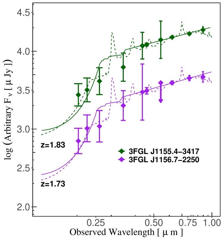
Figure 1: The Swift-UVOT +SARA spectral energy distribution of the two high-$z$ sources. The ($solid~{}line$) power law templates are fitted for each source with a clearly seen dropout towards the shorter wavelengths. In addition, the ($dashed~{}line$) galaxy template fits to these objects are presented. The redshifts estimates provided by the latter fits suggest $z=1.5$ for each source. The details of the fitting method and the inference of these results are described in Section  4. and  5., respectively.

4 SED fitting

Under the assumption that the spectral energy distribution (SED) does not change with flux changes from UV-Opt-nearIR regime for the BL Lacs and that it is a dominated by the non-thermal synchrotron emission, the 10 filter data obtained in this work could be assumed to follow a power-law spectrum (typical of BL Lacs). The fitting program, was utilized to determine the photometric redshifts. This program is based on the $\chi^{2}$ statistics for evaluating the difference between the observational and theoretical models. It should be noted that this program includes the response curves for all the filters. Therefore, the red leaks for UVW1 and UVW2 are taken into account during the fitting procedure. In the context of this work, we employed three different libraries to fit our data. The first library consisted of 60 power-law templates of the form $F_{\lambda}\propto\lambda^{-\beta}$. The value of $\beta$ was chosen to be in the range 0 to 3, since the typical indices for BL Lacs in this wavelength regime are in the above mentioned range. The dropout from the typical power-law fitting was employed to estimate the redshifts. The second and the third libraries comprised of galaxy and stellar templates, respectively, were also fit to check any false associations. The galaxy templates were derived from Salvato et al. (2009, 2011) and the stellar templates were obtained from Pickles (1998); Bohlin et al. (1995) and Chabrier et al. (2000).
Rau et al. (2012) performed Monte Carlo simulations for 27000 test SEDs with $\beta$ between 0.5-2.0 and redshifts from 0 to 4, in order to test the reliability of this fitting procedure to determine the photometric redshifts. These simulations yielded that the sources with redshifts greater than 1.2 reproduced the results within an accuracy of$\left|\Delta z(1+z_{sim})\right|<0.15$. Another selection criteria for measuring the reliability of redshift estimates were based on the integral of the probability distribution function, P${}_{z}=\int f(z)dz$ at $z_{phot}\pm 0.1(1+z_{phot})$. The resulting values with $P_{z}>90\%$ were considered reliable for this work.

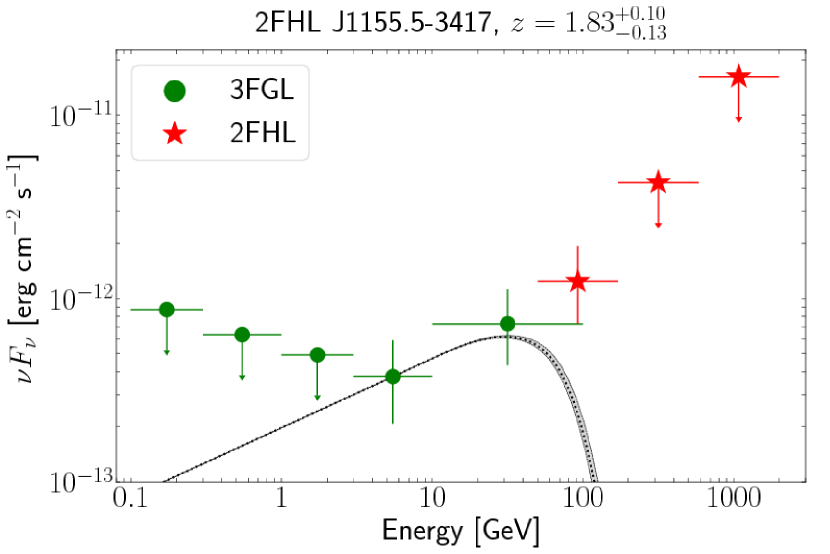
Figure 2: Spectral energy distribution of 3FGL J1155.4-3417 using the 3FGL and 3FHL catalogs. The black line is a power law fit to the 3FHL data, which is absorbed by the EBL, utilizing Domínguez et al. (2011).

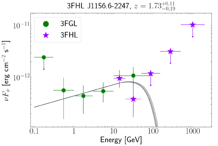
Figure 3: Spectral energy distribution of 3FGL J1156.6-2247 using the 3FGL and 3FHL catalogs. The black line is a power law fit to the 3FHL data, which is absorbed by the EBL, utilizing Domínguez et al. (2011).

5 Results

The SED fitting results were assessed for reliability based on the two criteria mentioned in the previous section, i.e. $z\geq 1.3$ and $P_{z}>90\%$. From our sample of 15 sources, we found two at redshifts greater than 1.3, which is consistent with our predicted rate of 10-15% of the sources being at high redshifts, as indicated by our previous studies (Rau et al., 2012) and (Kaur et al., 2017). Swift-UVOT + SARA SEDs of these two objects, 3FGL J1155.5$+$3417 and 3FGL J1156.6$-$2247, are shown in Fig. 1. The redshifts for these two BL Lacs were found to be $z=1.83^{+0.10}_{-0.13}$ and $z=1.73^{+0.11}_{-0.19}$, respectively, using the powerlaw template fits. In addition, galaxy templates were fit to these data, which yielded redshifts estimates, $z=1.50^{+0.02}_{-0.03}$ and $z=1.50^{+0.04}_{-0.07}$ assuming hybrid QSO templates from Salvato et al. (2011). Both the sources, 3FGL J1155.5-3417 and 3FGL J1156.6-2250 are identified as BL Lac (D’Abrusco et al., 2014) and HSP BCU II (Ackermann et al., 2015) (associated with the BL Lac class), respectively, therefore the redshifts estimates provided by the QSO templates with prominent broad emission lines are rather unlikely. Moreover, the QSO templates yield redshifts estimates without including any fit to the optical emission lines (See Fig. 1), we therefore assume the redshift estimated provided by the powerlaw fits to be more precise. Therefore the rest of the analysis will be based on the redshift estimates derived from powerlaw fits . Moreover, upper limits for 4 sources were established. All these results are presented in Table 3. None of the sources in our sample were consistent with the stellar templates used for the SED fitting, therefore those results are not displayed in Table 3.
The outcome of the combined analysis of BL Lac observations taken at different epochs can be affected by spectral variability. To verify our findings of two new high-z sources, we obtained new observations for these two sources using $Swift$ and SARA simultaneously on 2017-12-28 and 2017-12-27, respectively. The results of this analysis yielded $z=1.73^{+0.11}_{-0.15}$ and $z=1.83^{+0.12}_{-0.15}$ for 3FGL J1155.5$+$3417 and 3FGL J1156.6$-$2247, respectively, which are consistent with our archival data analysis, within the uncertainties.

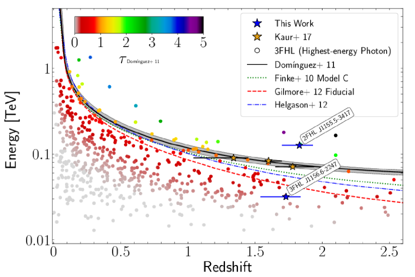
Figure 4: The Cosmic $\gamma$-ray horizon plot: The highest energy of photons from sources (with E $>$ 50 GeV) vs. their redshift . The colors of sources imply their corresponding optical depth ($\tau$) values (see colorbar). Various estimates of the cosmic $\gamma$-ray horizon, obtained from the EBL models by Finke et al. (2010, dotted green line), Domínguez et al. (2011, solid black line, with uncertainties as shaded band), Gilmore et al. (2012, dashed red line) and Helgason & Kashlinsky (2012, dot-dashed blue line) are plotted for comparison. The highest energy photons from one of the two high-$z$ sources lie above the cosmic $\gamma$-ray horizon ($blue~{}filled~{}stars$), whereas the other source lies below this limit. The three $orange$ star symbols represent the high-$z$ BL Lacs found in Rau et al. (2012) and Kaur et al. (2017), for which 2FHL data were available.

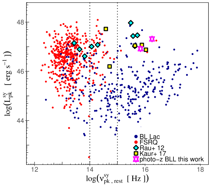
Figure 5: The peak synchrotron frequency in the rest frame ($\nu_{sy}^{pk}$) vs the peak synchrotron luminosity ($L_{sy}^{pk}$). The magenta stars represent the two new sources found in the present work. These are consistent with the other high-$z$ BL Lacs using photometric method, which display the high luminosity and high synchrotron peak behavior. We show 6 new BL Lacs from Rau et al. (2012, cyan diamonds), 5 BL Lacs from Kaur et al. (2017, yellow squares), and all the FSRQs and BL Lacs from the 3LAC catalog with known redshifts (red and blue circles, respectively). The separation of the LSP, ISP, and HSP regions are also plotted (dotted lines).

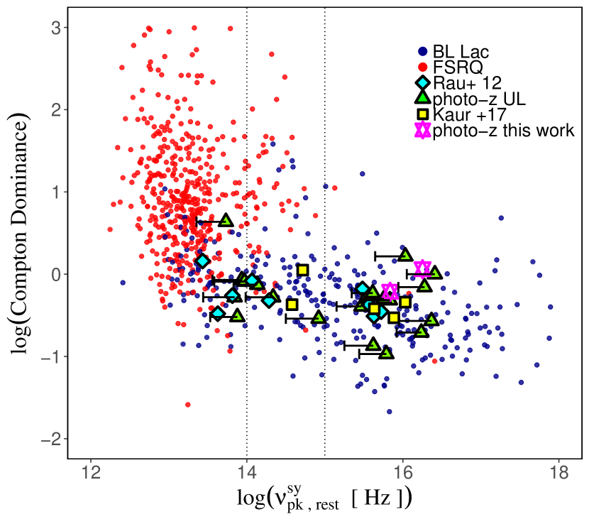
Figure 6: The relationship between the Compton Dominance and $\nu_{sy}^{\rm pk}$. The color scheme for data symbols follows from Figure 5. All the upper limits, including the ones from this work are represented in green $filled$ triangles. The black $horizontal$ lines represent the range of $\nu_{sy}^{pk}$ for redshifts from zero to the upper limits, provided in our sample.

6 Discussion and Conclusions

The two newly discovered high-$z$ BL Lacs are also part of the recent third catalog of high-energy sources (3FHL, Ajello et al., 2017, 3FGL J1155.5+3417 is also present in the 2FHL Ackermann et al. (2016) catalog). Therefore, we utilized the 3FGL and 3FHL catalogs to construct the SEDs of these two sources. These were fitted with a power law with an EBL absorption of form, $e^{-\tau(E,z)}$ using the Domínguez et al. (2011) model as illustrated in Fig. 2 and 3. These fits indicates that the observed flux at high energies from these two sources was reduced by a factor of $\sim$ 10, due to the EBL absorption, in both cases. We also reproduced the cosmic gamma ray horizon plot (i.e. the redshift at which, for a given energy, the Universe becomes opaque to $\gamma$ rays, see Domínguez et al. (2013) using all the sources in the 3FHL catalog and including the two new sources found here. This is displayed in Fig. 4, which shows that the photometric method is able to find $\gamma$-ray sources that can constrain the cosmic $\gamma$-ray horizon (CGRH), which is defined by the energy at which the optical depth $\tau$ is one as a function of redshift, at redshifts where data are scarce. Interestingly, the highest energy photon from J1155.4$-$3417 lies above the CGRH with $\tau\approx 2.8$. The objects discovered with our photometric technique (the two reported here and also those in Rau et al., 2012; Kaur et al., 2017) allow us to probe a region of the cosmic $\gamma$-ray horizon where measurements are scarce and as such they allow us to better constrain the EBL. Indeed, the detection of many high-energy photons above the horizon may imply that the EBL model used may be too opaque to characterize the real level of the EBL in the Universe. In the case of Fig. 4, the model of Gilmore et al. (2012) is less favored (because more opaque) than the one of Domínguez et al. (2011). To understand how these high-$z$ BL Lacs fit within the larger blazar population (Maraschi et al., 1995; Sambruna et al., 1996; Fossati et al., 1998), we calculated various parameters like the synchrotron peak frequency $\nu_{sy}^{pk}$, the luminosity at the synchrotron peak ($L_{sy}^{pk}$) and the Compton Dominance (CD, the ratio between the luminosities of the inverse Compton and synchrotron peaks). Fossati et al. (1998) observed some correlations between the above mentioned parameters using the available blazar data. This sequence indicates that the more luminous blazars possess lower synchrotron frequencies, but substantial $\gamma$-ray emission (FSRQs in general), whereas BL Lacs are less luminous, but achieve larger synchrotron peak frequencies. We test these correlations by plotting all the blazars in the 3LAC catalog, together with the high-$z$ BL Lacs discovered in all our photometric campaigns. Fig. 5 suggests the presence of large luminosity-high frequency synchrotron peak blazars, which do not fit very well with the known blazar sequence scheme. Although, in order to draw a more robust conclusion in this scenario, a larger sample of such sources is required. Fig. 6 displays peak synchrotron frequency vs compton dominance and shows that all our BL Lacs display CD $\leq$ 1, which is consistent with the typical SED of this subclass of blazars, suggesting a more dominant synchrotron emission.
Including the results of this work, our continuing photometric method has discovered 13 BL Lacs. Overall, 26 (including 2 found here) BL Lacs are known in the literature with $z>1.3$, of which 50% were provided by us. Moreover, the accuracy of this method was shown in Fig.2 in Kaur et al. (2017) by successfully matching the spectroscopic and photometric redshifts estimates for the BL Lacs.

In the present 3LAC catalog (Ackermann et al., 2013), about 300 BL Lacs lack redshift measurements. The primary objective of our photometric program is to provide the redshifts or at least the upper limits for the 3LAC catalog for all the BL Lacs. Based on the previous results, this work has yielded a total of 16 sources (9 (6 new) from Rau et al. (2012), 5 from Kaur et al. (2017), 2 from this work) with high redshifts from sample sizes of 103, 40 and 15, respectively. Based on the probability of finding 10-15% of BL Lacs at the high redshifts from our samples, we estimate to obtain 30-35 more high-$z$ BL Lacs from the 3LAC catalog which has $\sim$ 300 BL Lacs with no redshifts measurements. This will provide a total number of $\sim$ 50 high-$z$ BL Lacs, leading to the completion of this work and more importantly, will provide a large enough sample of BL Lacs at high redshifts for EBL studies.

Table 1: Swift-UVOT and SARA Observations

3FGL	Swift	RA J2000	Dec J2000	Swift Datea	SARA Datea	$A_{V}$
(Name)	(Name)	(hh:mm:ss)	(${}^{\circ}:^{\prime}:^{\prime\prime}$)	(UT)	(UT)	(mag)
J0305.2$-$1607	PKS 0302$-$16	03:05:15.04	$-$16:08:16.3	2011$-$01$-$07.96	2016$-$12$-$04.2	0.12
J0703.4$-$3914	NVSS J070312$-$391418	07:03:12.66	$-$39:14:18.9	2011$-$12$-$06.64	2016$-$12$-$01.1	0.35
J0855.2$-$0718	3C 209	08:55:58.31	$-$07:26:36.9	2011$-$10$-$26.93	2016$-$12$-$01.2	0.09
J0947.1$-$2542	1RXS J094709.2$-$254056	09:47:09.50	$-$25:41:00.0	2013$-$10$-$06.80	2016$-$12$-$04.3	0.20
J1155.4$-$3417	2FHL J1155.5$-$3417	11:55:20.47	$-$34:17:19.9	2016$-$07$-$26.80	2017$-$02$-$18.1	0.22
J1156.7$-$2250	1WHSP J115633.2$-$225004	11:56:33.20	$-$22:50:04.5	2016$-$11$-$24.15	2017$-$02$-$18.2	0.13
J1218.8$-$4827	PMN J1219$-$4826	12:19:02.270	$-$48:26:28.1	2013$-$06$-$26.88	2017$-$01$-$25.2	0.33
J1518.0$-$2732	TXS 1515$-$273	15:18:3.59	$-$27:31:30.6	2014$-$09$-$30.87	2017$-$03$-$21.2	0.22
J1723.7$-$7713	TAN 1716$-$771	17:23:50.81	$-$77:33:50.5	2011$-$05$-$13.81	2017$-$03$-$21.2	0.70
J1759.1$-$4822	PMN J1758$-$4820	17:58:58.45	$-$48:21:12.4	2013$-$08$-$17.70	2017$-$03$-$21.3	0.55
J1841.2+2910	2WHSP J184121.7+290940	18:41:21.70	+29:09:41.0	2015$-$12$-$10.86	2017$-$07$-$14.0	0.64
J1911.4$-$1908	PMN J1911$-$1908	19:11:29.73	$-$19:08:24.5	2014$-$07$-$30.45	2017$-$06$-$09.2	0.43
J1955.0$-$1605	1RXS J195500.6$-$160328	19:55:00.58	$-$16:03:37.9	2014$-$08$-$06.98	2017$-$06$-$09.3	0.56
J2031.0+1937	RX J2030.8+1935	20:30:57.13	+19:36:1	2014$-$06$-$01.54	2017$-$07$-$14.1	0.25
J2336.5$-$7620	PMN J2336$-$7620	23:36:27.59	$-$76:20:37.8	2014$-$07$-$19.39	2017$-$07$-$10.4	0.19

Table 2: Swift-UVOT and SARA photometry

3FGL Name	$g^{\prime}$	$r^{\prime}$	$i^{\prime}$	$z^{\prime}$	$uvw2$	$uvm2$	$uvw1$	$u$	$b$	$v$
J0305.2$-$1607	$>$20.89	18.96$\pm$ 0.06	18.40$\pm$ 0.06	18.68$\pm$ 0.17	22.24$\pm$ 0.12	21.99 $\pm$ 0.14	21.98$\pm$ 0.16	21.61$\pm$ 0.19	21.29$\pm$ 0.26	$>$ 20.84
J0703.4$-$3914	18.71$\pm$ 0.03	17.54$\pm$ 0.01	15.76$\pm$ 0.02	16.38$\pm$ 0.03	20.42$\pm$ 0.12	20.46 $\pm$ 0.18	20.16$\pm$ 0.17	19.31$\pm$ 0.12	18.93$\pm$ 0.14	18.61$\pm$ 0.19
J0855.2$-$0718	19.87$\pm$ 0.12	18.93$\pm$ 0.05	18.34$\pm$ 0.08	18.86$\pm$ 0.28	22.09$\pm$ 0.22	21.37 $\pm$ 0.24	20.86$\pm$ 0.17	20.40$\pm$ 0.19	20.04$\pm$ 0.25	$>$ 19.61
J0947.1$-$2542	16.74$\pm$ 0.02	16.50$\pm$ 0.01	17.41$\pm$ 0.01	16.49$\pm$ 0.03	17.73$\pm$ 0.06	17.75 $\pm$ 0.08	17.45$\pm$ 0.07	17.09$\pm$ 0.06	16.77$\pm$ 0.07	16.78$\pm$ 0.12
J1155.4$-$3417	18.19$\pm$ 0.02	17.95$\pm$ 0.01	17.84$\pm$ 0.02	17.72$\pm$ 0.04	19.80$\pm$ 0.14	19.64 $\pm$ 0.15	19.36$\pm$ 0.17	18.91$\pm$ 0.18	18.22$\pm$ 0.17	18.03$\pm$ 0.24
J1156.7$-$2250	19.17$\pm$ 0.04	18.91$\pm$ 0.02	18.76$\pm$ 0.03	18.73$\pm$ 0.07	20.77$\pm$ 0.16	20.37 $\pm$ 0.17	20.30$\pm$ 0.20	19.64$\pm$ 0.19	19.20$\pm$ 0.36	$>$ 18.91
J1218.8$-$4827	17.24$\pm$ 0.04	16.46$\pm$ 0.02	16.44$\pm$ 0.02	16.10$\pm$ 0.04	18.58$\pm$ 0.09	18.56 $\pm$ 0.18	18.17$\pm$ 0.10	18.01$\pm$ 0.12	17.38$\pm$ 0.11	17.39$\pm$ 0.18
J1518.0$-$2732	17.44$\pm$ 0.12	16.51$\pm$ 0.03	16.20$\pm$ 0.04	15.97$\pm$ 0.07	18.67$\pm$ 0.09	18.75 $\pm$ 0.11	18.46$\pm$ 0.12	17.81$\pm$ 0.10	17.60$\pm$ 0.14	16.97$\pm$ 0.14
J1723.7$-$7713	18.42$\pm$ 0.05	17.99$\pm$ 0.02	17.92$\pm$ 0.03	17.53$\pm$ 0.06	19.35$\pm$ 0.22	$>$ 19.79	19.34$\pm$ 0.28	$>$ 19.33	18.49$\pm$ 0.29	$>$ 17.86
J1759.1$-$4822	15.57$\pm$ 0.04	13.03 $\pm$ 0.02	15.24 $\pm$ 0.03	15.26$\pm$ 0.06	$>$ 17.87	$>$ 17.52	$>$ 17.33	$>$ 16.97	16.17$\pm$ 0.31	$>$ 15.65
J1841.2+2910	16.83$\pm$ 0.01	17.09$\pm$ 0.01	17.10$\pm$ 0.01	16.90$\pm$ 0.03	18.14$\pm$ 0.18	$>$18.57	17.57$\pm$ 0.18	17.37$\pm$ 0.20	16.77$\pm$ 0.19	$>$16.90
J1911.4$-$1908	18.24$\pm$ 0.03	17.62$\pm$ 0.01	17.30$\pm$ 0.01	16.97$\pm$ 0.02	19.83$\pm$ 0.27	19.73 $\pm$ 0.26	$>$19.46	18.69$\pm$ 0.27	18.34$\pm$ 0.29	17.66$\pm$ 0.36
J1955.0$-$1605	17.72$\pm$ 0.05	17.35$\pm$ 0.02	17.04$\pm$ 0.02	16.69$\pm$ 0.03	19.02$\pm$ 0.20	$>$19.22	18.35$\pm$ 0.26	18.17$\pm$ 0.20	17.77$\pm$ 0.24	$>$ 17.58
J2031.0+1937	17.52$\pm$ 0.01	17.93$\pm$ 0.01	17.75$\pm$ 0.01	17.57$\pm$ 0.04	18.33$\pm$ 0.13	18.45 $\pm$ 0.24	18.17$\pm$ 0.19	17.50$\pm$ 0.17	17.45$\pm$ 0.30	$>$16.95
J2336.5$-$7620	18.06$\pm$ 0.05	16.53$\pm$ 0.02	17.34$\pm$ 0.03	17.24$\pm$ 0.08	19.74$\pm$ 0.16	19.43 $\pm$ 0.22	19.12$\pm$ 0.17	18.82$\pm$ 0.18	18.35$\pm$ 0.20	18.18$\pm$ 0.32

Table 3: SED fitting

3FGL Name	$z_{\rm phot,best}^{a}$	Power Law Template				Galaxy Template
		$z_{\rm phot}$ b	$\chi^{2}$	P${}_{\rm z}^{c}$	$\beta^{d}$	$z_{\rm phot}$ b	$\chi^{2}$	Pz c	model
Sources with confirmed photometric redshifts
J1155.4$-$3417	${1.83}^{+0.10}_{-0.13}$	${1.83}^{+0.10}_{-0.13}$	20.0	99.9	0.65	${1.50}^{+0.02}_{-0.03}$	28.8	100.0	pl_QSOH_template_norm.sed
J1156.7$-$2250	${1.73}^{+0.11}_{-0.19}$	${1.73}^{+0.11}_{-0.19}$	9.2	98.5	0.70	${1.50}^{+0.04}_{-0.07}$	7.1	99.9	pl_QSOH_template_norm.sed
Sources with photometric redshifts upper limits
J0305.2$-$1607	$\cdots$	${0.85}^{+0.01}_{-0.18}$	565.2	45.8	0.80	${1.22}^{+0.03}_{-0.02}$	297.3	93.6	S0_template_norm.sed
J0703.4$-$3914	$\cdots$	${4.00}^{+0.00}_{-0.01}$	267.6	100.0	0.45	${0.61}^{+0.04}_{-0.05}$	25.4	89.5	Sey2_template_norm.sed
J0855.2$-$0718	$\cdots$	${3.86}^{+0.00}_{-0.00}$	128.0	82.3	1.10	${0.45}^{+0.05}_{-0.01}$	39.3	99.9	M82_template_norm.sed
J0947.1$-$2542	$\cdots$	${1.63}^{+0.10}_{-0.08}$	70.6	99.9	0.45	${1.33}^{+0.05}_{-0.04}$	24.9	63.6	pl_TQSO1_template_norm.sed
J1218.8$-$4827	$\cdots$	${1.23}^{+0.21}_{-0.60}$	181.7	50.9	1.40	${0.26}^{+0.01}_{-0.01}$	28.8	100.0	pl_QSOH_template_norm.sed
J1518.0$-$2732	$<$1.1	${0.05}^{+1.03}_{-0.05}$	22.9	16.8	1.85	${0.19}^{+0.10}_{-0.06}$	11.07	98.0	Mrk231_template_norm.sed
J1723.7$-$7713	$\cdots$	${2.74}^{+0.21}_{-0.04}$	44.3	99.5	0.80	${0.01}^{+0.03}_{-0.01}$	19.8	99.8	Spi4_template_norm.sed
J1759.1$-$4822	$\cdots$	${3.86}^{+0.00}_{-0.00}$	$\cdots$	$\cdots$	$\cdots$	$\cdots$	$\cdots$	$\cdots$	$\cdots$
J1841.2+2910	$\cdots$	${2.06}^{+0.08}_{-0.10}$	176.7	100.0	$\cdots$	${0.45}^{+0.03}_{-0.01}$	244.9	100.0	S0_80_QSO2_20.sed
J1911.4$-$1908	$<$1.6	${1.33}^{+0.28}_{-1.33}$	21.2	41.0	1.60	${0.06}^{+0.03}_{-0.02}$	7.1	100.0	Mrk231_template_norm.sed
J1955.0$-$1605	$<$1.2	${0.03}^{+1.13}_{-0.03}$	25.7	13.6	1.65	${1.26}^{+0.04}_{-0.03}$	36.2	100.0	I22491_90_TQS01_10.sed
J2031.0+1937	$\cdots$	${2.03}^{+0.10}_{-0.08}$	247.8	100.0	$\cdots$	${1.93}^{+0.02}_{-0.05:w}$	255.9	100.0	I22491_70_TQS01_20.sed
J2336.5$-$7620	$<$1.5	${1.33}^{+0.22}_{-0.11}$	9.5	60.8	1.35	${0.08}^{+0.05}_{-0.04}$	8.9	100.0	Spi4_template_norm.sed

References

- Abdo et al. (2010) Abdo, A. A., Ackermann, M., Ajello, M., et al. 2010, The Astrophysical Journal, 723, 1082
- Abdo et al. (2011a) —. 2011a, The Astrophysical Journal, 727, 129
- Abdo et al. (2011b) —. 2011b, The Astrophysical Journal, 736, 131
- Acero et al. (2015) Acero, F., Ackermann, M., Ajello, M., et al. 2015, The Astrophysical Journal Supplement Series, 218, 23
- Ackermann et al. (2012) Ackermann, M., Ajello, M., Allafort, A., et al. 2012, Science (New York, N.Y.), 338, 1190
- Ackermann et al. (2013) —. 2013, The Astrophysical Journal Supplement Series, 209, 34
- Ackermann et al. (2015) Ackermann, M., Ajello, M., Atwood, W. B., et al. 2015, The Astrophysical Journal, 810, 14
- Ackermann et al. (2016) —. 2016, The Astrophysical Journal Supplement Series, 222, 5
- Aharonian et al. (2006) Aharonian, F., Akhperjanian, A. G., Bazer-Bachi, A. R., et al. 2006, Nature, 440, 1018
- Ajello et al. (2017) Ajello, M., Atwood, W. B., Baldini, L., et al. 2017, The Astrophysical Journal Supplement Series, 232, 18
- Arnouts et al. (1999) Arnouts, S., Cristiani, S., Moscardini, L., et al. 1999, Monthly Notices of the Royal Astronomical Society, 310, 540
- Blandford & Rees (1978) Blandford, R. D., & Rees, M. J. 1978, Physica Scripta, 17, 265
- Bohlin et al. (1995) Bohlin, R. C., Colina, L., & Finley, D. S. 1995, The Astronomical Journal, 110, 1316
- Chabrier et al. (2000) Chabrier, G., Baraffe, I., Allard, F., & Hauschildt, P. 2000, The Astrophysical Journal, 542, 464
- Crespo et al. (2016) Crespo, N. Á., Massaro, F., Milisavljevic, D., et al. 2016, The Astronomical Journal, Volume 151, Issue 4, article id. 95, 10 pp. (2016)., 151, 95
- D’Abrusco et al. (2014) D’Abrusco, R., Massaro, F., Paggi, A., et al. 2014, The Astrophysical Journal Supplement Series, 215, 14
- Domínguez & Ajello (2015) Domínguez, A., & Ajello, M. 2015, The Astrophysical Journal Letters, Volume 813, Issue 2, article id. L34, 4 pp. (2015)., 813, arXiv:1510.07913
- Domínguez et al. (2013) Domínguez, A., Finke, J. D., Prada, F., et al. 2013, The Astrophysical Journal, 770, 77
- Domínguez et al. (2011) Domínguez, A., Primack, J. R., Rosario, D. J., et al. 2011, Monthly Notices of the Royal Astronomical Society, 410, 2556
- Finke et al. (2010) Finke, J. D., Razzaque, S., & Dermer, C. D. 2010, The Astrophysical Journal, 712, 238
- Fossati et al. (1998) Fossati, G., Maraschi, L., Celotti, A., Comastri, A., & Ghisellini, G. 1998, Monthly Notices of the Royal Astronomical Society, 299, 433
- Gehrels et al. (2004) Gehrels, N., Chincarini, G., Giommi, P., et al. 2004, The Astrophysical Journal, 611, 1005
- Gilmore et al. (2012) Gilmore, R. C., Somerville, R. S., Primack, J. R., & Domínguez, A. 2012, Monthly Notices of the Royal Astronomical Society, 422, 3189
- Giommi et al. (2011) Giommi, P., Padovani, P., Polenta, G., et al. 2011, Monthly Notices of the Royal Astronomical Society, Volume 420, Issue 4, pp. 2899-2911., 420, 2899
- Greiner et al. (2008) Greiner, J., Bornemann, W., Clemens, C., et al. 2008, Publications of the Astronomical Society of the Pacific, 120, 405
- Hauser & Dwek (2001) Hauser, M. G., & Dwek, E. 2001, Annual Review of Astronomy and Astrophysics, Vol. 39, p. 249-307 (2001)., 39, 249
- Helgason & Kashlinsky (2012) Helgason, K., & Kashlinsky, A. 2012, The Astrophysical Journal Letters, Volume 758, Issue 1, article id. L13, 6 pp. (2012)., 758, arXiv:1208.4364
- Ilbert et al. (2006) Ilbert, O., Arnouts, S., McCracken, H. J., et al. 2006, Astronomy and Astrophysics, 457, 841
- Kataoka et al. (2008) Kataoka, J., Madejski, G., Sikora, M., et al. 2008, The Astrophysical Journal, 672, 787
- Kaur et al. (2017) Kaur, A., Rau, A., Ajello, M., et al. 2017, The Astrophysical Journal, Volume 834, Issue 1, article id. 41, 10 pp. (2017)., 834, 41
- Keel et al. (2016) Keel, W. C., Oswalt, T., Mack, P., et al. 2016, Publications of the Astronomical Society of Pacific, Volume 129, Issue 971, pp. 015002 (2017)., 129, 015002
- Kolb (2002) Kolb, U. 2002, The Physics of Cataclysmic Variables and Related Objects, 261, 180
- Krühler et al. (2011) Krühler, T., Schady, P., Greiner, J., et al. 2011, Astronomy & Astrophysics, 526, A153
- Landt (2012) Landt, H. 2012, Monthly Notices of the Royal Astronomical Society: Letters, 423, doi:10.1111/j.1745-3933.2012.01262.x
- Maraschi et al. (1995) Maraschi, L., Fossati, G., Tagliaferri, G., & Treves, A. 1995, The Astrophysical Journal, 443, 578
- Marcha & I. W. A. (1996) Marcha, M. J. M., & I. W. A., B. 1996, Monthly Notices of the Royal Astronomical Society, 279, 72
- Massaro et al. (2015) Massaro, F., Landoni, M., D’Abrusco, R., et al. 2015, Astronomy & Astrophysics, Volume 575, id.A124, 24 pp., 575, doi:10.1051/0004-6361/201425119
- Pickles (1998) Pickles, A. J. 1998, Publications of the Astronomical Society of the Pacific, 110, 863
- Poole et al. (2007) Poole, T. S., Breeveld, A. A., Page, M. J., et al. 2007, Monthly Notices of the Royal Astronomical Society, 383, 627
- Rau et al. (2012) Rau, A., Schady, P., Greiner, J., et al. 2012, Astronomy & Astrophysics, 538, A26
- Roming et al. (2005) Roming, P. W. A., Kennedy, T. E., Mason, K. O., et al. 2005, Space Science Reviews, 120, 95
- Salvato et al. (2009) Salvato, M., Hasinger, G., Ilbert, O., et al. 2009, The Astrophysical Journal, 690, 1250
- Salvato et al. (2011) Salvato, M., Ilbert, O., Hasinger, G., et al. 2011, The Astrophysical Journal, 742, 61
- Sambruna et al. (1996) Sambruna, R. M., Maraschi, L., & Urry, C. M. 1996, The Astrophysical Journal, 463, 444
- Schlafly & Finkbeiner (2011) Schlafly, E. F., & Finkbeiner, D. P. 2011, The Astrophysical Journal, 737, 103
- Shaw et al. (2013a) Shaw, M. S., Filippenko, A. V., Romani, R. W., Cenko, S. B., & Li, W. 2013a, The Astronomical Journal, 146, 127
- Shaw et al. (2013b) Shaw, M. S., Romani, R. W., Cotter, G., et al. 2013b, The Astrophysical Journal, 764, 135
- Stecker et al. (1992) Stecker, F. W., de Jager, O. C., & Salamon, M. H. 1992, The Astrophysical Journal, 390, L49
- Tody & Doug (1986) Tody, D., & Doug. 1986, in IN: Instrumentation in astronomy VI; Proceedings of the Meeting, Tucson, AZ, Mar. 4-8, 1986. Part 2 (A87-36376 15-35). Bellingham, WA, Society of Photo-Optical Instrumentation Engineers, 1986, p. 733., ed. D. L. Crawford, Vol. 627, 733
- Urry & Padovani (1995) Urry, C. M., & Padovani, P. 1995, Publications of the Astronomical Society of the Pacific, 107, 803