A Systematic Chandra study of Sgr A^⋆: II. X-ray flare statistics

Abstract

The routinely flaring events from Sgr A^⋆ trace dynamic, high-energy processes in the immediate vicinity of the supermassive black hole. We statistically study temporal and spectral properties, as well as fluence and duration distributions, of the flares detected by the Chandra X-ray Observatory from 1999 to 2012. The detection incompleteness and bias are carefully accounted for in determining these distributions. We find that the fluence distribution can be well characterized by a power-law with a slope of $1.73^{+0.20}_{-0.19}$, while the durations ($\tau$ in seconds) by a log-normal function with a mean $\log(\tau)=3.39^{+0.27}_{-0.24}$ and an intrinsic dispersion $\sigma=0.28^{+0.08}_{-0.06}$. No significant correlation between the fluence and duration is detected. The apparent positive correlation, as reported previously, is mainly due to the detection bias (i.e., weak flares can be detected only when their durations are short). These results indicate that the simple self-organized criticality model has difficulties in explaining these flares. We further find that bright flares usually have asymmetric lightcurves with no statistically evident difference/preference between the rising and decaying phases in terms of their spectral/timing properties. Our spectral analysis shows that although a power-law model with a photon index of $2.0\pm 0.4$ gives a satisfactory fit to the joint spectra of strong and weak flares, there is weak evidence for a softer spectrum of weaker flares. This work demonstrates the potential to use statistical properties of X-ray flares to probe their trigger and emission mechanisms, as well as the radiation propagation around the black hole.

1 Introduction

Low-luminosity supermassive black holes (LL-SMBHs) represent the silent majority ($\sim 90\%$) of SMBHs in our Universe. Sgr A^⋆ is in a rather steady low-luminosity state, referred to as the “quiescent state”, with peak emission in the sub-millimeter band. Occasionally there are substantial variations in the emission, known as flares, which are most prominent in the (near) infrared (NIR/IR) and X-ray bands (Genzel et al., 2003; Baganoff et al., 2001). The spatial, spectral, and temporal decompositions of the X-ray emission of Sgr A^⋆ show that 1) the quiescent emission is mostly extended and the flaring emission is point-like (Baganoff et al., 2003; Wang et al., 2013); 2) there is an additional point-like, super-soft quiescent component which are not accounted for by detected flares (Roberts et al., 2017); 3) the spectrum is optically thin thermal for the quiescent extended emission while featureless power-laws for flares (Baganoff et al., 2001; Nowak et al., 2012; Wang et al., 2013); 4) the rate of X-ray flares is about $1\sim 2$ per day (Ponti et al., 2015; Yuan & Wang, 2016) or about $3$ per day after correcting for the detection threshold (Mossoux & Grosso, 2017), which is a factor of a few smaller than that of NIR/IR ones (Eckart et al., 2006).

The quiescent emission of Sgr A^⋆ can be explained in terms of the radiatively inefficient inflow/outflow model (Yuan, Quataert & Narayan, 2003; Narayan et al., 2012; Wang et al., 2013; Yuan et al., 2015; Roberts et al., 2017). The origin of the flares is, however, still unclear. From the temporal spectral properties, crucial information regarding the radiative mechanisms associated with the flares can be extracted. However, existing studies tended to focus on individual strong flares detected with reasonably good counting statistics, mostly via observations made with XMM-Newton (Porquet et al., 2003; Bélanger et al., 2005; Yusef-Zadeh et al., 2006; Porquet et al., 2008) and a few with Chandra (Baganoff et al., 2001; Nowak et al., 2012) and NuSTAR (Barrière et al., 2014; Ponti et al., 2017). Only a few works studied the flare population, with limited flare samples (Neilsen et al., 2013; Zhang et al., 2017). Moreover, the spectral shape of such flares is often modeled by an absorbed power-law. Comparison among the photon indices ($\Gamma$) obtained for various flares is therefore not straightforward, when $\Gamma$ is strongly correlated with the foreground absorption column density $N_{\rm H}$ in the spectral fits. There could be differences in the modeling of such details due to adoption of different versions of the absorption cross-sections, dust absorption/scattering, and/or metal abundance pattern. For bright flares detected by Chandra, pile-up effects, which include the grade migration (Davis, 2001), can be problematic, as they cause distortion in the spectra data. Whether or not, and/or how the pile-up is treated can therefore affect the values of the photon indices when fitting the spectral data. With these in consideration, one finds that essentially all flares can be consistently characterized with a power law of $\Gamma\simeq 2$ and $N_{H}\simeq 1.5\times 10^{23}{\rm~{}cm^{-2}}$ of neutral material (Porquet et al., 2008; Nowak et al., 2012). This column density would be slightly smaller when dust scattering is accounted for separately. Nevertheless, the studies of NuSTAR flares which extended the spectral coverage beyond 10 keV (up to about 70 keV; Barrière et al., 2014) and Swift ones (Degenaar et al., 2013), do sometimes show that they may have different photon indices (e.g., $\Gamma\sim 3$). In this work, we extend the spectral analysis to relatively faint flares by both measuring hardness ratios (HRs) of individual flares and fitting to stacked data.

Flare statistics, on the other hand, may provide insights into the driving mechanism and how flares are triggered. It has been argued that flares are associated with the ejection of plasma blobs triggered by magnetic reconnection (e.g. Yusef-Zadeh et al., 2006). One of the magnetic reconnection scenarios is that the system shows characteristics of self-organized criticality (SOC). In it, a critical state is reached gradually by nonlinear energy buildup, followed by an avalanche energy release, which manifests as a flaring event (e.g., Katz, 1986; Bak, Tang & Wiesenfeld, 1987). In such a SOC flaring model, if the system is scale-free, the total energy released in the flare, the peak rate of energy dissipation, and the flaring time duration should all obey a power-law distribution, and the slopes of these three power laws are determined by the effective geometric dimension of the system (Aschwanden, 2012; Aschwanden et al., 2016). SOC models have been applied to explain the statistics of flares in the Sun (e.g., Lu & Hamilton, 1991; Aschwanden, 2011), and in astrophysical black-hole systems (Wang & Dai, 2013; Li et al., 2015), The 3-Ms data of Sgr A^⋆ obtained in the Chandra X-ray Visionary Project (XVP) (Neilsen et al., 2013) have shown that the X-ray flaring statistics of the source are consistent with those predicted by SOC models with a spatial dimension $S=3$ (Wang et al., 2015; Li et al., 2015). However, the analyses might be limited by a relatively small sample of flares with narrow fluence range and by lacking a proper account for incompleteness and bias in the flare detection, the results obtained should be taken with caution.

Yuan & Wang (2016, hereafter Paper I) have presented a systematical search for X-ray flares in 84 Chandra observations of Sgr A^⋆. Fourty-six of these observations were taken before 2012, using the Advanced CCD Imaging Spectrometer - Imaging array (ACIS-I), while the other 38 in 2012, using the Advanced CCD Imaging Spectrometer - Spectroscopy array with the high energy transmission gratings (ACIS-S/HETG0, where “0” refers to the non-dispersed zeroth order). Chandra observations taken after 2012 are not included in the search because of the varying appearance of the X-ray bright magnetar, SGR J1745-2900 (Kennea et al., 2013), just $2.4^{\prime\prime}$ away from Sgr A^⋆, which complicates the detection and statistical analysis of Sgr A^⋆ flares. With an improved unbinned likelihood method, the search finds a total of 82 flares in the $\sim 4.5$ Ms observations, about 1/3 of which are newly detected ones (see Tables 1 and  2 for a sub-sample with relatively low pile-up effect). These two Chandra samples of Sgr A^⋆ flares form the base for the statistical analysis presented here. In addition, the detection incompleteness, uncertainty and bias are carefully studied for the first time, which is especially important for a statistical analysis including weak flares close to the detection threshold, as is the case for the work reported here. We adopt the detection response matrices, as obtained in Paper I, to better characterize the detection effects on the flare statistics.

Table 1: Properties of the ACIS-I flares used for spectral analysis.

FlareID	$\log(F/{\rm cts})$	$\log(\tau/{\rm ks})$	$t_{\rm start}$	$t_{\rm end}$	$F_{\rm pileup}$
			(ks)	(ks)
I1	$1.07\pm 0.23$	$0.45\pm 0.20$	54270.053	54274.283	1.00
I2	$1.35\pm 0.12$	$0.03\pm 0.12$	89000.851	89002.455	0.93
I3	$1.00\pm 0.26$	$0.14\pm 0.29$	130520.43	130522.51	1.00
I4	$0.82\pm 0.30$	$-0.04\pm 0.41$	133277.53	133278.89	1.00
I5	$1.85\pm 0.10$	$0.80\pm 0.09$	138651.24	138659.31	1.00
I6	$1.72\pm 0.09$	$0.60\pm 0.11$	138771.38	138777.35	0.98
I7	$1.02\pm 0.19$	$0.01\pm 0.26$	138781.96	138783.49	1.00
I8	$1.49\pm 0.12$	$0.64\pm 0.14$	138805.22	138811.78	1.00
I9	$1.39\pm 0.12$	$0.18\pm 0.09$	138864.21	138866.47	0.95
I10	$1.09\pm 0.18$	$0.23\pm 0.21$	138877.64	138880.18	1.00
I11	$2.18\pm 0.07$	$0.76\pm 0.10$	139036.87	139044.73	0.92
I12	$0.94\pm 0.24$	$-0.14\pm 0.61$	139464.54	139465.62	1.00
I13	$1.17\pm 0.22$	$0.47\pm 0.24$	172451.56	172455.98	1.00
I14	$0.92\pm 0.21$	$-0.20\pm 0.28$	205542.87	205543.81	0.99
I15	$1.77\pm 0.08$	$0.83\pm 0.09$	239074.25	239084.39	1.00
I16	$1.15\pm 0.17$	$0.30\pm 0.21$	265566.39	265569.39	1.00
I17	$1.07\pm 0.19$	$0.32\pm 0.16$	275579.64	275582.78	1.00
I18	$1.14\pm 0.15$	$0.30\pm 0.16$	305152.20	305155.20	1.00
I19	$0.99\pm 0.26$	$-0.49\pm 0.51$	326370.81	326371.29	0.91
I20	$1.14\pm 0.21$	$0.51\pm 0.26$	333497.06	333501.92	1.00
I21	$1.21\pm 0.18$	$0.36\pm 0.26$	333503.03	333506.47	1.00
I22	$1.78\pm 0.12$	$0.55\pm 0.19$	359001.19	359005.59	0.95
I23	$1.90\pm 0.12$	$0.61\pm 0.09$	359026.86	359032.09	0.94
I24	$1.28\pm 0.14$	$0.39\pm 0.13$	417781.80	417785.48	1.00

Note: Columns from left to right are: flare ID, logarithmic flare fluence, logarithmic flare duration, start and end times from UT 1998-01-01 00:00:00, which define the flare intervals, and pile-up correction factor.

Table 2: Properties of the ACIS-S/HETG0 flares used for spectral analysis.

FlareID	$\log(F/{\rm cts})$	$\log(\tau/{\rm ks})$	$t_{\rm start}$	$t_{\rm end}$	$F_{\rm pileup}$
			(ks)	(ks)
S1	$1.94\pm 0.05$	$0.49\pm 0.05$	453264.94	453269.58	0.93
S2	$1.82\pm 0.11$	$0.30\pm 0.10$	453933.00	453935.77	0.92
S3	$1.85\pm 0.06$	$0.59\pm 0.05$	459317.44	459323.28	0.95
S4	$1.85\pm 0.09$	$0.94\pm 0.08$	459428.50	459438.92	1.00
S5	$2.09\pm 0.04$	$0.60\pm 0.03$	460110.73	460116.71	0.92
S6	$2.01\pm 0.08$	$0.51\pm 0.11$	460253.06	460257.06	0.92
S7	$2.24\pm 0.06$	$0.82\pm 0.10$	467370.02	467380.57	0.93
S8	$1.18\pm 0.13$	$0.27\pm 0.14$	445170.33	445173.11	1.00
S9	$1.37\pm 0.11$	$-0.10\pm 0.09$	448630.66	448631.84	0.92
S10	$1.38\pm 0.11$	$0.12\pm 0.10$	448633.82	448635.80	0.95
S11	$1.37\pm 0.11$	$0.19\pm 0.10$	448638.60	448640.92	0.96
S12	$1.55\pm 0.08$	$0.59\pm 0.08$	452260.13	452265.97	1.00
S13	$1.43\pm 0.11$	$0.40\pm 0.14$	452746.05	452749.81	1.00
S14	$1.36\pm 0.11$	$0.67\pm 0.13$	452774.14	452781.16	1.00
S15	$1.41\pm 0.18$	$0.86\pm 0.58$	453136.68	453143.17	1.00
S16	$1.27\pm 0.12$	$0.47\pm 0.13$	453168.52	453172.94	1.00
S17	$1.10\pm 0.21$	$0.64\pm 0.32$	453192.47	453199.03	1.00
S18	$1.00\pm 0.18$	$0.32\pm 0.19$	453821.66	453824.80	1.00
S19	$1.11\pm 0.15$	$0.20\pm 0.15$	453937.72	453940.09	1.00
S20	$1.06\pm 0.17$	$0.47\pm 0.15$	453944.22	453948.64	1.00
S21	$1.56\pm 0.08$	$0.74\pm 0.07$	459039.34	459047.59	1.00
S22	$1.16\pm 0.14$	$0.43\pm 0.12$	459057.69	459061.73	1.00
S23	$1.39\pm 0.11$	$0.09\pm 0.14$	459176.29	459178.13	0.94
S24	$1.03\pm 0.15$	$-0.09\pm 0.14$	459217.17	459218.39	0.99
S25	$1.36\pm 0.11$	$0.02\pm 0.10$	459380.52	459382.10	0.94
S26	$1.47\pm 0.09$	$0.04\pm 0.08$	459508.28	459509.93	0.93
S27	$0.95\pm 0.18$	$-0.29\pm 0.19$	459605.82	459606.58	0.95
S28	$1.27\pm 0.13$	$0.55\pm 0.14$	459860.71	459866.03	1.00
S29	$0.96\pm 0.28$	$0.55\pm 0.33$	459873.61	459878.93	1.00
S30	$1.41\pm 0.10$	$0.73\pm 0.09$	460040.91	460048.97	1.00
S31	$0.86\pm 0.20$	$-0.05\pm 0.23$	460268.82	460270.16	0.99
S32	$1.60\pm 0.08$	$0.13\pm 0.05$	460452.53	460454.55	0.92
S33	$1.57\pm 0.10$	$1.24\pm 0.09$	460482.85	460508.95	1.00
S34	$1.37\pm 0.10$	$0.52\pm 0.13$	460539.33	460544.29	1.00
S35	$1.30\pm 0.12$	$0.40\pm 0.13$	460781.60	460785.36	1.00
S36	$1.22\pm 0.15$	$0.54\pm 0.17$	465968.67	465973.87	1.00
S37	$1.40\pm 0.10$	$0.38\pm 0.09$	466057.06	466060.66	1.00
S38	$0.74\pm 0.24$	$-0.14\pm 0.25$	466827.00	466828.08	1.00
S39	$1.20\pm 0.13$	$0.34\pm 0.19$	466970.77	466974.05	1.00
S40	$1.19\pm 0.24$	$0.88\pm 0.34$	467413.12	467424.50	1.00
S41	$1.59\pm 0.12$	$0.38\pm 0.10$	467529.97	467533.23	0.96
S42	$1.66\pm 0.08$	$0.84\pm 0.10$	467965.49	467975.87	1.00
S43	$0.83\pm 0.19$	$-0.03\pm 0.19$	468004.79	468006.19	1.00
S44	$1.49\pm 0.10$	$0.51\pm 0.14$	468076.64	468081.50	1.00

Note: Same as Table 1. The central horizontal line separates the strong flares from the weak ones.

To provide further constraints on the nature of the flares, we statistically characterize their time profiles and spectral variations. There have been a few studies on such properties of a few individual bright flares (e.g. Baganoff et al., 2001; Porquet et al., 2003; Bélanger et al., 2005; Yusef-Zadeh et al., 2006; Porquet et al., 2008; Nowak et al., 2012; Degenaar et al., 2013; Barrière et al., 2014; Ponti et al., 2017). We extend these studies to relatively weak flares, e.g., via stacking analysis.

The organization for the rest of this paper is as follows. In Section 2 we present the statistical analysis of the X-ray flares. The implications of our results in understanding the nature of the flares are briefly discussed in Section 3. Finally we summarize our work in Section 4.

2 Flare statistics

2.1 Fluence and duration distributions

This analysis follows the approach of Li et al. (2015) to characterize the probability distributions of the flare fluence ($F$) and duration ($\tau$). The distribution of $F$ is assumed to be a power-law, $P(F)=A\cdot F^{-\alpha}$, while $\tau$ follows a log-normal function, $N(\log\tau;\mu,\sigma)$, in which $\mu=\log(B\cdot F^{\beta})$ is the expected mean correlation with the fluence and $\sigma$ is the Gaussian width of $\log\tau$. Hereafter we use $\log F$ and $\log\tau$ as variables. The joint intrinsic probability distribution of the fluence ($\log F_{i}$) and duration ($\log\tau_{i}$) is then

$$P(\log F_{i},\log\tau_{i}) = P(\log F_{i})\cdot P(\log\tau_{i}|\log F_{i})$$

$$= F_{i}\cdot\ln 10\cdot P(F_{i})\cdot N(\log\tau_{i};\log B+\beta\log F_{i},\sigma).$$

The joint probability distribution of the detectedfluence ($\log F_{d}$) and duration ($\log\tau_{d}$) is

$$P(\log F_{d},\log\tau_{d})=P(\log F_{d},\log\tau_{d};\,\log F_{i},\log\tau_{i})\otimes P(\log F_{i},\log\tau_{i}),$$ (2)

where $\otimes$ means the convolution of $P(\log F_{i},\log\tau_{i})$ with $P(\log F_{d},\log\tau_{d};\,\log F_{i},\log\tau_{i})$, which is a redistribution matrix. It is obtained through Monte Carlo simulations for the two flare samples separately, accounting for the counting statistics and background-dependent detection incompleteness and bias (see Paper I). Individual flares are considered to be independent Poisson realizations. The logarithmic likelihood function of our $N_{d}$ detected flare is then (Cash, 1979)

$$\ln{\mathcal{L}}(\vec{\theta}|{\rm Data})=\sum_{k}^{N_{d}}\ln P(\log F^{k}_{d},\log\tau^{k}_{d})-N_{\rm pred},$$ (3)

where $\vec{\theta}=(A,\alpha,B,\beta,\sigma)$ represent the model parameters, the sum is over all the detections ($k=1,...,N_{d}$) and

$$N_{\rm pred}=\int\int P(\log F_{d},\log\tau_{d})\,{\rm d}\log F_{d}\,{\rm d}\log\tau_{d}$$ (4)

is the expected total number of flares. We use the Markov Chain Monte Carlo (MCMC) method to maximize Eq. (3) and constrain the model parameters $\vec{\theta}$. Compared with Paper I, we improve the flare statistical study through proper considerations of the Poisson fluctuation and the detection bias in a joint fit of the fluence distribution and the fluence-duration correlation.

Table 3 gives the best-fit and posterior two-sided $95\%$ confidence ranges of the parameters. The corresponding 1-dimensional (1-d) and 2-dimensional (2-d) distributions of the fitting parameters are shown in Figure 1. The parameters obtained for the ACIS-I and -S/HETG0 flares are consistent with each other.

Table 3: The best-fit, posterior mean values and the 95% limits of the logarithmic normalization ($\log A$) and power-law index ($\alpha$) of the fluence distribution, and the logarithmic normalization ($\log B$), power-law index ($\beta$), and dispersion width ($\sigma$) of the fluence-duration correlation (see § 2.1).

$\log A$

$\alpha$

$\log B$

$\beta$

$\sigma$

best

posterior mean

best

posterior mean

best

posterior mean

best

posterior mean

best

posterior mean

and 95% limits

and 95% limits

and 95% limits

and 95% limits

and 95% limits

ACIS-I

2.13

$2.26_{-0.55}^{+0.56}$

1.68

$1.77_{-0.32}^{+0.33}$

3.34

$3.38_{-0.38}^{+0.46}$

0.09

$0.08_{-0.23}^{+0.21}$

0.25

$0.28_{-0.09}^{+0.15}$

ACIS-S/HETG0

2.24

$2.29_{-0.40}^{+0.46}$

1.71

$1.75_{-0.24}^{+0.28}$

3.35

$3.45_{-0.41}^{+0.53}$

0.10

$0.05_{-0.30}^{+0.26}$

0.28

$0.32_{-0.09}^{+0.13}$

Joint fit

2.22

$2.23\pm 0.29$

1.72

$1.73_{-0.19}^{+0.20}$

3.38

$3.39_{-0.24}^{+0.27}$

0.09

$0.08_{-0.17}^{+0.15}$

0.28

$0.28_{-0.06}^{+0.08}$

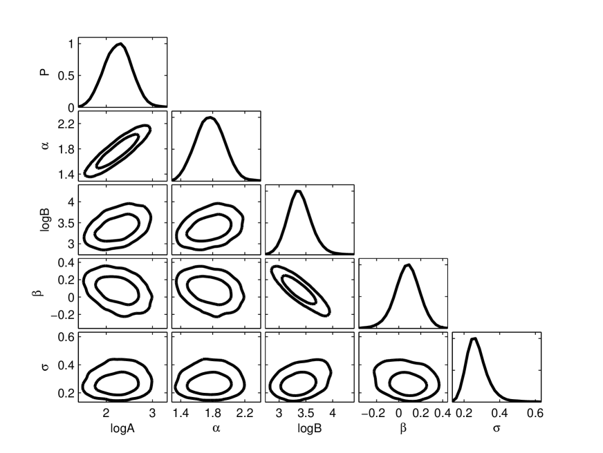
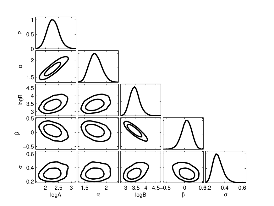
Figure 1: Fitting 1-d (diagonal) probability distributions and 2-d (off-diagonal) contours at 68% and 95% confidence levels of the model parameters, $(\log A,\alpha,\log B,\beta,\sigma)$, for the ACIS-I (left) and -S/HETG0 (right) data.

The top two panels of Figure 2 show the detection probability distribution as a function of $\log F_{d}$ and $\log\tau_{d}$ (Eq. 2) for the best-fit models of the two flare samples, respectively. As a comparison, we show in the bottom two panels the intrinsic probability distribution without the convolution with the detection redistribution matrix. It clearly shows how an apparent correlation can be obtained from an intrinsically nearly uncorrelated distribution between the fluence and duration. The detection redistribution matrix makes long duration, weak flares undetectable and the probability distribution wider.

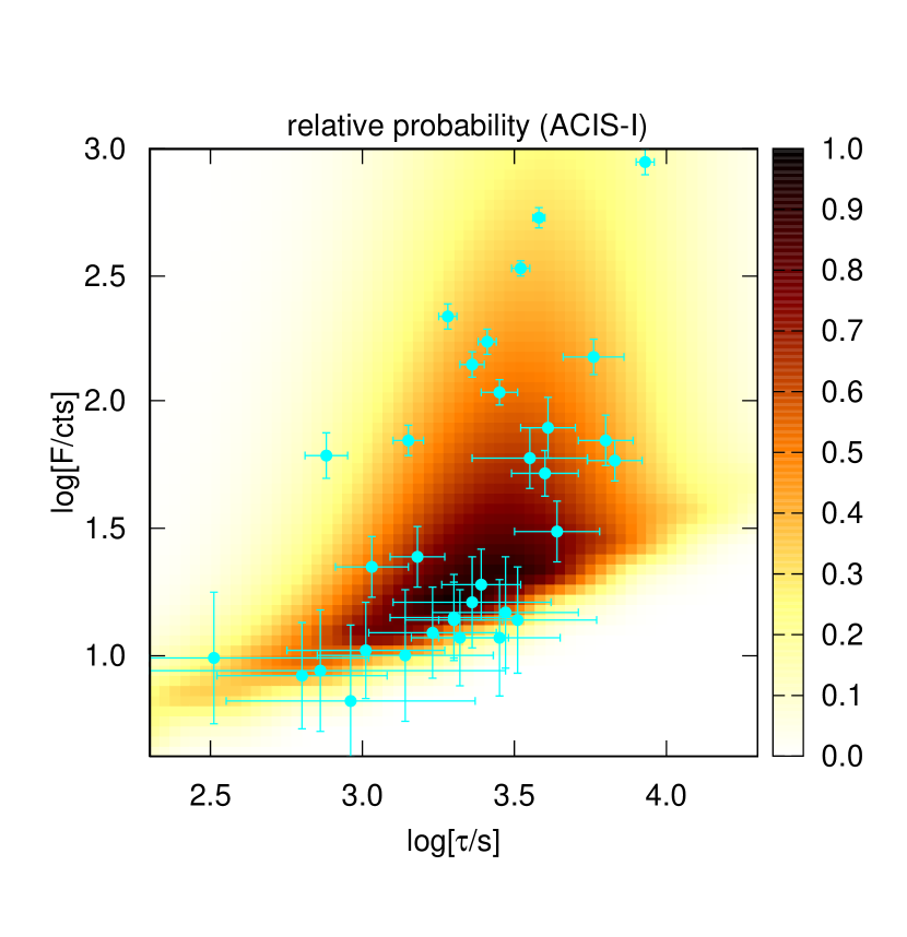
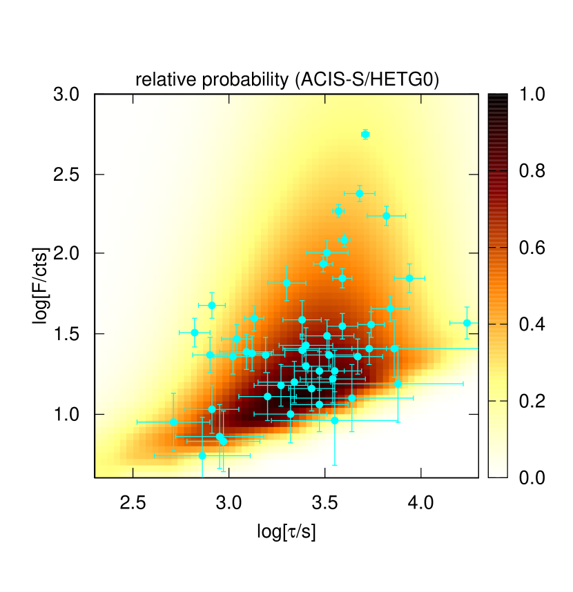
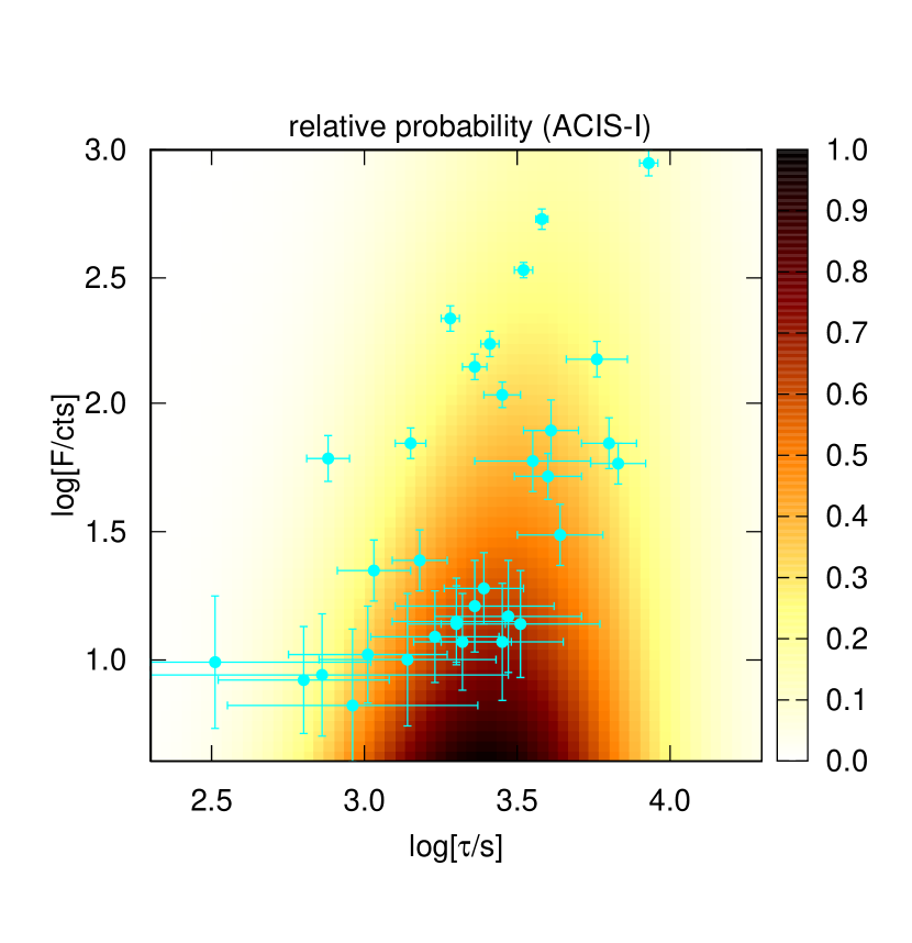
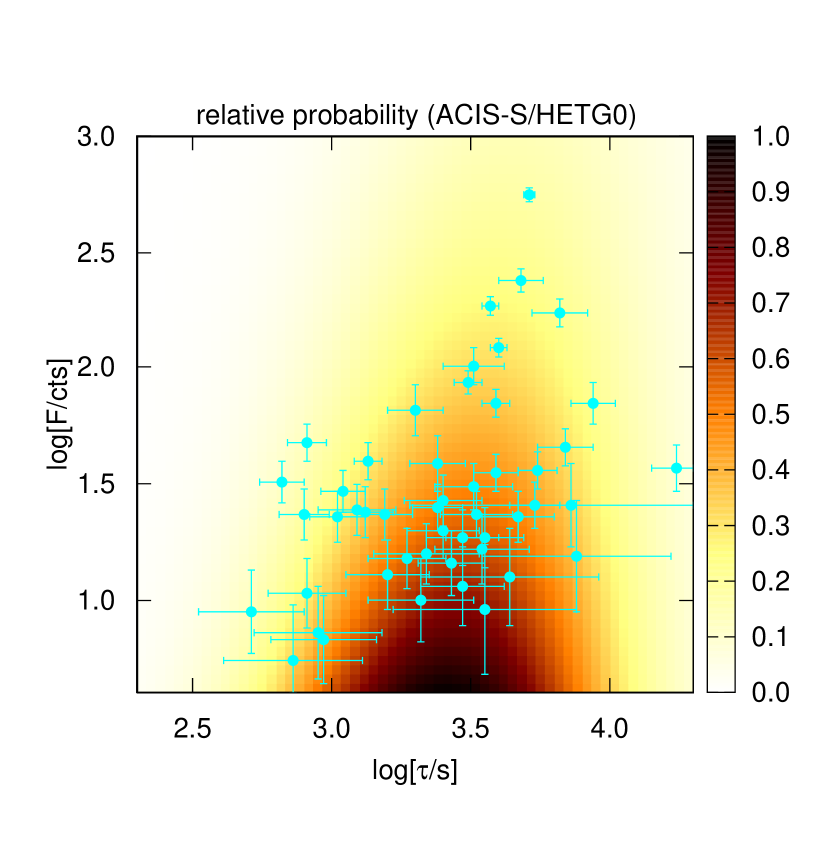
Figure 2: The images in the top two panels show the relative probability distributions of the flare detection as a function of the fluence and duration, for the ACIS-I (left) and -S/HETG0 (right) samples. The overlaid data points are from our detected flares in the respective samples (Paper I). For comparison, the images in the bottom two panels show the intrinsic probability distributions of flares without convolution with the redistribution matrices.

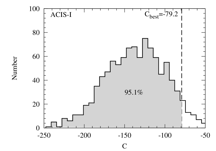
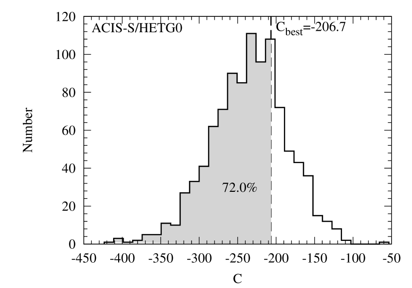
Figure 3: Distributions of the $C$-statistic values (defined as $-2\ln{\mathcal{L}}$) of the fits to the 1000 sets of statistically realized flares, following the best-fit fluence-duration distributions, for the ACIS-I (left) and -S/HETG0 (right) samples.

We assess the goodness of the fit to the detected flares from each of the two detected flare samples via bootstrapping sampling. Figure 3 present the distributions of $C\equiv-2\ln{\mathcal{L}}$ from the fits to the 1000 sets of bootstrapped flares, which are randomly realized from the best-fit model. The number fraction with $C$ smaller than that of the actual data ($C_{\rm best}=-206.7$) is $72\%$ for the ACIS-S/HETG0 flares, suggesting that the data are well described by the model. The corresponding fraction is $95.1\%$ for the ACIS-I data, which means a slightly worse fitting.

We further jointly fit the two flare samples to improve the constraints on the model parameters. Since the effective area (exposure time) of the ACIS-I observations is on average a factor of $\sim 2.6$ ($2.0$) larger (smaller) than that of the ACIS-S/HETG0 observations (Paper I), we expect to have $P(F_{I})=P(F_{S})\cdot{\rm d}F_{S}/{\rm d}F_{I}\cdot t_{I}/t_{S}$, and hence $A_{I}=A_{S}\cdot 2.6^{\alpha-1}/2$, where the subscription “_I” (“_S”) stands for the ACIS-I (-S/HETG0) flares. Similarly for the fluence-duration correlation we have $B_{I}=B_{S}/2.6^{\beta}$. The joint fit significantly tightens the constraints on the model parameters, which are included in Table 3.

The power-law index of the fluence distribution, $\alpha\sim 1.7$, is consistent with those found in Neilsen et al. (2013) and Li et al. (2015). But we find little intrinsic correlation between the fluence and duration ($\beta\sim 0$), although an apparent correlation is present for the detected flares (e.g., Figure 1; Paper I; Neilsen et al., 2013; Li et al., 2015). Such correlations are largely due to the detection bias and uncertainty, which were not fully accounted for previously.

2.2 Flare time profiles

We characterize the asymmetry properties of flare time profiles. In Paper I we used only the standard symmetric Gaussian profiles to approximate the flare lightcurves. Here we relax this approximation for those “strong” flares, each with fluence $F>50$ counts. We adopt a modified Gaussian function of varying width (Stancik & Brauns, 2008)

$$\sigma(t)=\frac{2\sigma_{0}}{1+\exp[-\xi(t-t_{0})]}.$$ (5)

This function recovers to the standard Gaussian function with a constant width $\sigma_{0}$ when $\xi=0$. When $\xi>0$, the profile will be broader for $t>t_{0}$ and narrower for $t<t_{0}$, and vise versa when $\xi<0$.

We refit the lightcurves of the strong flares, using the function to derive the shape asymmetry parameter $\xi$. For consistency, the single function is applied in all fits, including those with indications for subflares, because their effects are generally too subtle to be effectively distinguished from those arising from the overall profile asymmetry. The results are shown in Figure 4, suggesting that about half of the flares have positive $\xi$ values (hence fast rise and slow decay) and the other half show negative $\xi$ (slow rise and fast decay). The number of the flares with positive $\xi$ is only slightly larger that that with negative $\xi$. There is no obvious trend of $\xi$ with respect to the fluence. A general anti-correlation is present between $\xi$ and the flare durations for both samples, although each has one exception, which has the shortest duration among the flares.

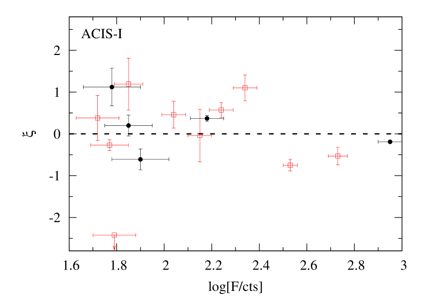
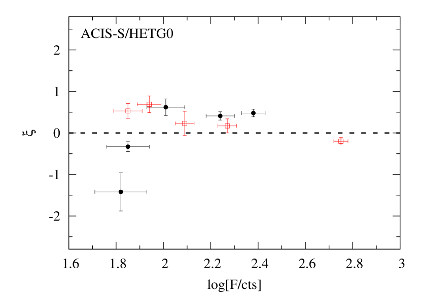
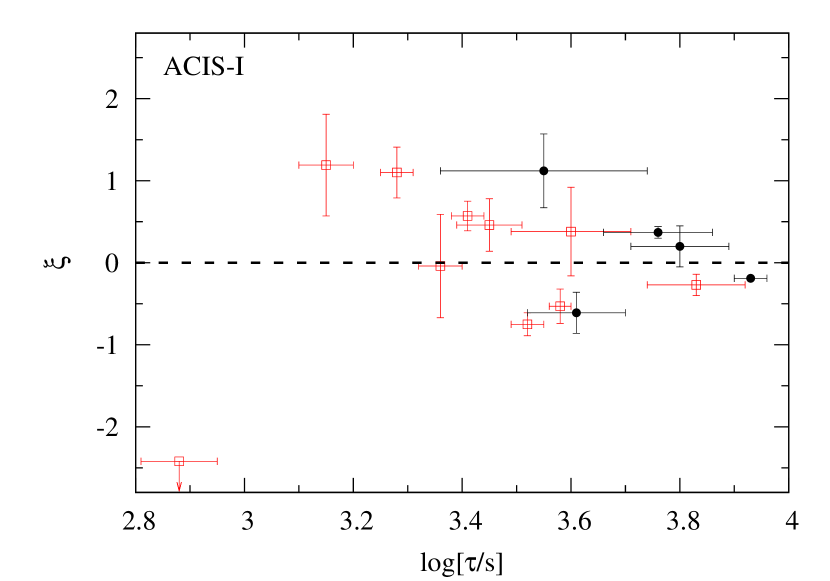
Figure 4: Top panels: the profile asymmetry parameter $\xi$ versus the fluence for our detected flares with $F>50$ cts in the ACIS-I (left) and -S/HETG0 (right) samples. Bottom panels: $\xi$ versus the duration of the same flares. Red squares are for isolate single flares, while black dots are for those with apparent multiple subflare signature (see Paper I).

2.3 Flare spectral propertiers

To characterize the spectral properties of a flare, we first define its spectral hardness ratio (HR) as

$${\rm HR}=\frac{N_{c}(4-8\,{\rm keV})}{N_{c}(2-4\,{\rm keV})},$$ (6)

where $N_{c}$ is the number of net (quiescent contribution-subtracted) counts accumulated within $\pm 3\sigma$ range of the Gaussian lightcurve. The event rate of the quiescent contribution below (above) 4 keV is calculated using the events detected over non-flaring time windows, which is 2.33 (2.55) cts/ks for the ACIS-I data and 0.73 (1.14) cts/ks for the -S/HETG0 data, respectively. Furthermore, to characterize the spectral evolution of a flare, we separate the counts into two parts, the rising phase before the best-fit Gaussian peak and the decaying phase after the peak. The results are given in Figure 5.

We adopt a linear function, ${\rm HR}=\lambda\cdot\log F+\eta$ (${\rm HR}=\mu\cdot\log P+\nu$), to characterize the correlation between the HR and logarithmic fluence $F$ (peak rate $P$) for the two flare samples. The fitting results are given in Tables 4 and 5. For the ACIS-I flares, a positive correlation is seen for both the rising (at a confidence level of $2\sim 3\sigma$) and decaying phases ($\sim 4\sigma$). For the ACIS-S/HETG0 flares, however, this correlation is less significant. Only for the rising phase we find a marginal correlation with a significnace of $\sim 2.4\sigma$ ($1.2\sigma$) for the HR-fluence (HR-peak-rate) correlation. The ACIS-I data suggest that brighter flares tend to have harder spectra than weaker ones, especially for the decaying phase. This trend is, however, not obvious for the ACIS-S/HETG0 flares.

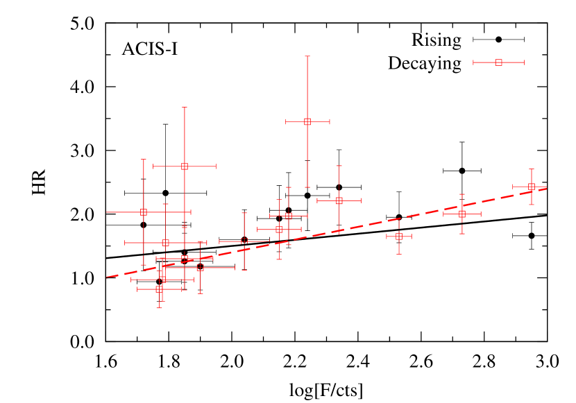
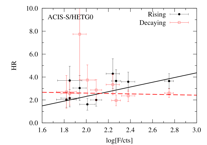
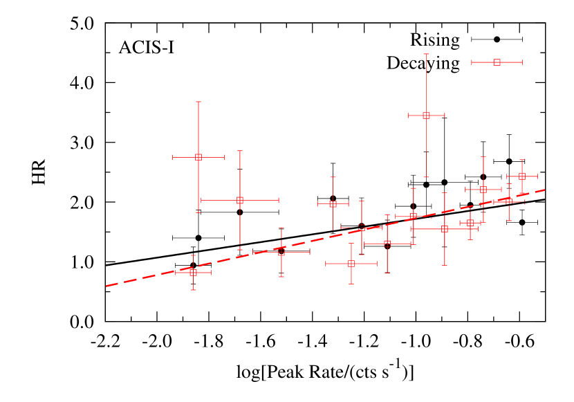
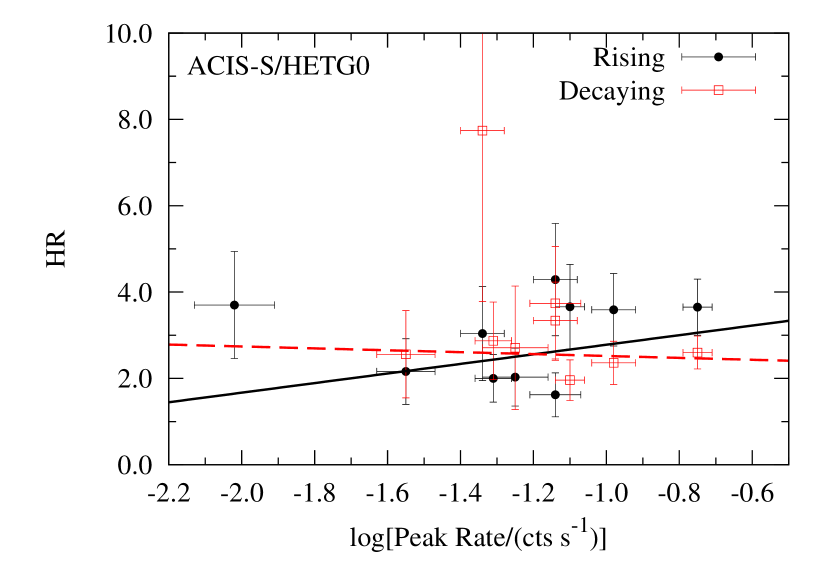
Figure 5: The HR versus the fluence (top panels) or peak rate (bottom panels) for the flares with $F>50$ cts in the ACIS-I (left) and -S/HETG0 (right) samples. Lines show the linear fits characterization of the correlation between the two parameters for the rising and decaying phases, separately.

Table 4: The best-fit values and $68\%$ uncertainties of the parameters characterizing the HR-fluence correlation ${\rm HR}=\lambda\cdot\log F+\eta$.

	Rising			Decaying
	$\lambda$	$\eta$		$\lambda$	$\eta$
ACIS-I	$0.48\pm 0.24$	$0.54\pm 0.56$		$1.00\pm 0.24$	$-0.60\pm 0.55$
ACIS-S/HETG0	$2.06\pm 0.83$	$-1.81\pm 1.77$		$-0.18\pm 0.79$	$2.96\pm 1.90$

Table 5: The best-fit values and $68\%$ uncertainties of the parameters characterizing the HR-peak-rate correlation ${\rm HR}=\mu\cdot\log P+\mu$.

	Rising			Decaying
	$\mu$	$\nu$		$\mu$	$\nu$
ACIS-I	$0.65\pm 0.24$	$2.37\pm 0.29$		$0.95\pm 0.25$	$2.68\pm 0.29$
ACIS-S/HETG0	$1.11\pm 0.94$	$3.89\pm 1.16$		$-0.22\pm 1.03$	$2.30\pm 1.05$

We next focus on the mean spectral properties of relative faint flares, based on the analysis of their accumulated spectra. We limit our spectral analysis to those flares with negligible pile-up effects, which are estimated from the analysis of the lightcurves of individual flares in a forward fitting procedure (Paper I). In principle, correction may also be made in spectral fits, using the pile-up model (Davis, 2001), as implemented in XSPEC. However, it is not clear how effective the correction may be for flares, which vary strongly. In any case, the correction, including at least one more fitting parameter, would introduce additional uncertainties in the spectral parameter estimation (Nowak et al., 2012). Therefore, we select those flares with the pile-up correction factor greater than 0.9 (i.e., the pile-up effect is $\lesssim 10\%$).

We use an aperture radius of $1^{\prime\prime}.5$ to extract spectral data of Sgr A^⋆. This extraction is made separately from the ACIS-I and -S/HETG0 observations. We extract on-flare spectral data from the time interval between the $\pm 3\sigma$ around the peak of each flare. If it contains subflares, then the interval is between their first $-3\sigma$ and last $+3\sigma$. We add the spectral data of individual flares together to form an accumulated spectrum. To examine potential flux dependent properties, we form two separate ACIS-S spectra from 7 strong and 37 weak flares, according to their individual fluences, greater or less than $10^{1.8}$ counts (Table 2). The corresponding ACIS-I fluence criterion is $10^{2.2}$ counts, due to the larger effective area. We find that all our 24 selected ACIS-I flares have fluences below this criterion (Table 1) and all have pile-up correction factors $<0.9$. We further construct two off-flare spectra of Sgr A^⋆, using the ACIS-I and -S/HETG0 data after excluding the time intervals of all the detected flares. These “quiescent” spectra are exposure-scaled and subtracted from the corresponding on-flare spectra in their analysis.

We fit the spectra with an absorbed power-law. Specifically, th XSPEC model tbabs is used to model the foreground absorption, which includes the contribution from dust grain (Wilms, Allen & McCray, 2000), while xscat to account for the grain scattering (Smith, Valencic & Corrales, 2016). The fitting is very insensitive to the location of the dust scattering. This parameter is thus fixed to 0.95 (i.e., close to Sgr A^⋆). A test inclusion of the pileup model shows that it has little effect on the best-fitting results, confirming our expectation.

The left panel of Figure 6 shows that the three spectra of the Sgr A^⋆ flares, i.e., the weak ACIS-I flares and the strong and weak ACIS-S ones, can be well fitted by a single absorbed power law ($\chi^{2}/n.d.f.=104/132$). The best fit photon index is $2.0\pm 0.4$, and the absorption column density is $N_{H}=13.5^{+3.1}_{-2.7}\times 10^{22}$ cm^-2. The uncertainties in these two parameters are largely due to their correlation, as shown in the right panel of Figure 6. To test any potential spectral dependence on the fluence of a flare. we first fix the column density to its best-fit value (i.e., removing the above mentioned uncertainties) and then fit the photon index for the strong flare spectrum independently, while keeping the indices of the other two spectra jointly fitted. This fit does show a marginal evidence that the weak flares have a slightly larger average index than that of the strong ones (Figure 7), which is consistent with the above HR analysis.

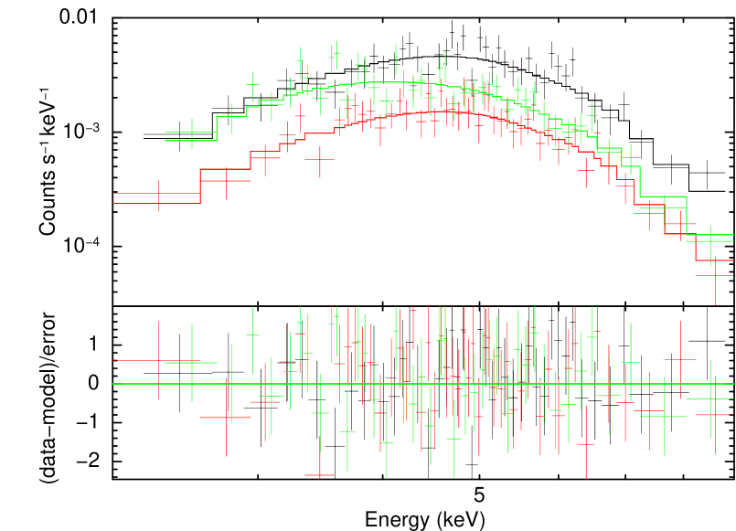
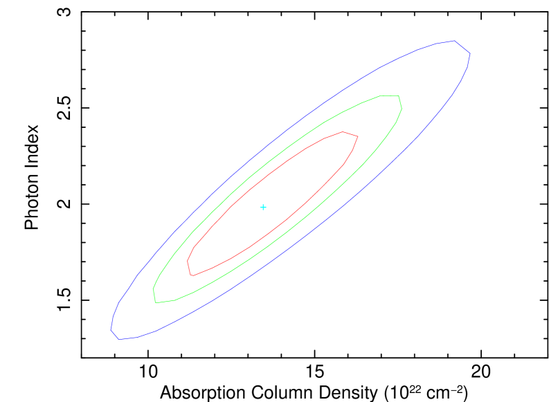
Figure 6: Left panel: joint power-law model fit to the Sgr A^⋆ flare spectra. They are accumulated for the strong (black) and weak (red) flares detected with the XVP ACIS-S/HETG0 data separately, as well as the flares detected with the ACIS-I data (green). The spectral contributions from the quiescent emission, estimated from the respective data, have been subtracted. Right panel: 68%, 90%, and 99% confidence contours of the power-law photon index versus the absorption column density of the fit.

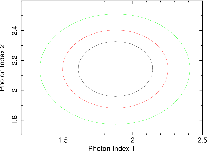
Figure 7: 68%, 90%, and 99% confidence contours of the two photon indiices for the strong flares (1) and the weak ones (2).

3 Discussion

The above results provide new insights on understanding the nature of the X-ray flare emission of Sgr A^⋆ and their origins, as well as indications for the possible relativistic and gravitational effects on the temporal and spectral properties of the flaring emission when propagating in the vicinity of the SMBH. We discuss these topics in the following.

3.1 Emission mechanism

We begin by a comparison of our spectral results with those obtained in previous studies, which are primarily focused on individual very bright flares. Ponti et al. (2017) showed that the average spectral index of three such flares observed by XMM-Newton is $\Gamma=2.20\pm 0.15$. Similar result was found for a sample of ten flares in a wider energy band of $1-79$ keV by NuSTAR (Zhang et al., 2017). These results are slightly steeper than, but still consistent within the 68% errors with that obtained here. There is an indication that strong flares tend to have harder spectra (Barrière et al., 2014; Zhang et al., 2017). See, however, Degenaar et al. (2013) for an opposite example. The result obtained in this work slightly favors the former one.

Starting from a generic point of view, we may consider that the X-rays from a flare are predominantly generated via a single radiative process. Collocated particles, presumably electrons, emit the polarised NIR/IR synchrotron radiation. As for the X-rays, bremsstrahlung (Liu & Melia, 2002), inverse Compton scattering (Yuan, Quataert & Narayan, 2003; Eckart et al., 2004; Liu et al., 2006; Marrone et al., 2008; Yusef-Zadeh et al., 2012) and synchrotron processes (Yuan, Quataert & Narayan, 2003, 2004; Dodds-Eden et al., 2009; Ponti et al., 2017), have been suggested as processes that give rise to the temporal and spectral behaviours observed in Sgr A^⋆.

The bremsstrahlung requires a large emission measure, and hence a high plasma density in the emission region. Although it is possible for a local pocket of high-density plasma (cf. plasmoids as in Yuan et al., 2009) to develop in an accretion inflow or outflow near the black hole through, for example, radiatively induced instabilities (see Liu & Melia, 2002), certain fine tuning is required in such bremsstrahlung models in order to explain the X-ray flares. The X-rays can also be produced when low-energy photons in the ambient field are Compton up-scattered by the energetic electrons that emit the polarised NIR/IR flare emission. During the flaring events the NIR/IR synchrotron photons dominate the radiation field in vicinity of Sgr A^⋆, thus the X-rays are a consequence of self-Comptonisation of the synchrotron radiation, i.e. an SSC process. As the X-rays and the NIR radiation are assumed to originate from the same region, combining the data obtained in the NIR and X-ray observations, one can constrain the effective source size and the particle density (Liu, Melia & Petrosian, 2006; Dodds-Eden et al., 2009). Analysis of a simultaneous NIR to X-ray flare by Dodds-Eden et al. (2009) showed that the SSC model yielded very extreme conditions for the emission region: an extremely small linear size (of $\sim 0.001-0.1$ Schwarzschild radius), a very strong magnetic field (of $\sim 10^{2}-10^{4}$ G) and a very high particle density (of $\sim 10^{8}-10^{12}\;\!{\rm cm}^{-3}$). The SSC model is therefore unlikely if NIR and X-ray flares are generated in the same location.

Simultaneous observations of a very bright flare from NIR to X-ray revealed a spectral break between the NIR and X-ray spectra with a difference of the slopes $\Delta\Gamma=0.57\pm 0.09$ (Ponti et al., 2017). One may argue that this points to synchrotron radiation in the presence of radiative cooling. However, the result must be interpreted with caution. If the NIR synchrotron flares are produced by the same population of electrons that are injected into the emission region as the X-ray ones and no efficient particle escape, we would expect a delay of NIR emission with respect to the X-ray one on the radiative cooling timescale. The observations do not support such a delay (Ponti et al., 2017).

For a homogeneous emission region with a single instantaneous particle injection, the effective cooling time can be estimated from the observed peak of the radiative spectrum $\nu_{\rm m}$, as $\tau_{\rm cool}=5\times 10^{11}(B\ \langle\sin\alpha\rangle)^{-3/2}\nu_{\rm m}^{-1/2}~{}{\rm sec}$ (see Tucker, 1975), where $B$ is the magnetic field threading the region and $\alpha$ is the pitch angle of the electrons with respect to the magnetic field. If we assume that $B\sim 10~{}{\rm G}$ (Dodds-Eden et al., 2009) and the electron momentum distribution is isotropic, for $\nu_{\rm m}\sim 10^{18}~{}{\rm Hz}$ we have $\tau_{\rm cool}\sim 0.75$ min. As the cooling time is much shorter than the duration of a flare, the acceleration (or injection) of electrons therefore cannot be due to an impulsive single event. The flare’s variability is therefore caused by the dynamical evolution of the system, with temporal variations in the injection process, if a single emission region dominates. Alternatively, spatial propagation of magnetic eruption fronts will lead to multiple injection/acceleration sites, giving rise to multiple emission regions.

Our analyses show no significant difference in the HRs between the rising and decaying phases (Figure 5), which does not support the shutdown of the flare being due to synchrotron cooling in a uniform plasma, because of the short cooling timescale and the anticipated dramatic spectral softening. Such persistence of the HR is however allowed, if the radiative particles escape from the region or the magnetic field dissipates. It is also allowed if the system is dynamical, with multiple particle injection/acceleration episodes and/or continuous particle injection/acceleration along a propagating magnetic reconnection front.

3.2 Origin of flares

We compare our improved statistical constraints on the fluence and duration distributions of the X-ray flares with the predictions of the various scenarios for the generation of Sgr A^⋆ X-ray flares. Among the broad class of magnetic reconnection scenarios for eruptive flares, SOC is a variant of the phenomenological models allowing a propagating front. The flare statistics in an SOC model depends on the effective geometric dimension of the system. For instance, a classical diffusion model predicts $\alpha_{\rm E}=3/2$ for the total energy (or the fluence) distribution, $\alpha_{\rm T}=2$ for the duration distribution, and $\beta=1/2$ for the duration-fluence correlation, for the spatial dimension of $S=3$ (Aschwanden et al., 2016). The observations of solar flares give on average $\alpha_{\rm E}=1.62\pm 0.12$ and $\alpha_{\rm T}=1.99\pm 0.35$, which are well consistent with the SOC predictions with $S=3$ (Aschwanden et al., 2016).

The (joint) statistical analysis of the X-ray flares in § 2.1 reveals that the fluence distribution slope is $\alpha\sim 1.7$, with the $95\%$ lower limit of $1.54$, which is considerably larger than the prediction of the simple SOC model for $S=3$. The duration versus fluence correlation is found to be very weak ($\beta\sim 0$). The $95\%$ upper limit of $\beta$ is about 0.23, which is substantially smaller than that (0.5) expected from the classical fractal diffusive SOC model. These results imply that the X-ray flares may not be self-similar, as predicted by the simple SOC model. It is possible that the non-uniform scenario of the SOC model with, e.g., finite boundary conditions, is responsible for such distributions of the flares. Alternatively, the X-ray fluence may not be a good measurement of the total energy of a flare.

A very different scenario for the production of Sgr A^⋆ flares is the tidal disruption of asteroids by the SMBH (e.g., Čadež, Calvani & Kostić, 2008; Kostić et al., 2009; Zubovas, Nayakshin & Markoff, 2012). Asteriods could be split into small pieces when passing close enough (e.g., within 1 AU) by the SMBH. They may then be vaporized by bodily friction with the accretion flow. A transient population of high-energy particles may be produced via the shock due to the bulk kinetic energy of an asteroid and/or plasma instabilities, leading to a flare of radiation (Zubovas, Nayakshin & Markoff, 2012). This asteroid disruption and evaporation model explains the luminosities, time scales and event rates of the flares, at least on the orders of magnitude. There is so far no clear prediction for the fluence distribution as well as the fluence-duration correlation of the model. However, in a very simple and rough analogy of the Galactic center environment to the Oort cloud of the solar system, one may assume that the size distribution of asteroids can be characterized by a power-law, $dn(r)/dr\propto r^{-q}$, with $q\sim 3-4$ (Zubovas, Nayakshin & Markoff, 2012). The fluence distribution of the flares simply follows the mass function of asteroids, which is $dn/dM\propto M^{(-q-2)/3}$. Therefore we have $\alpha\sim 1.7-2$, which is consistent with that obtained in our analysis (see Table 3). The typical duration of a flare is then determined by the flyby time of the asteroid, which is independent of the asteroid size (Zubovas, Nayakshin & Markoff, 2012). The predictions of the model are thus consistent with our observations. More detailed modeling of the asteroid distribution in the Galactic center environment, as well as the disruption and radiation processes of this scenario, is needed to further test its viability.

3.3 SMBH environment effect on the flare profile

Most of astronomical flaring events, such as the soft X-ray and lower-energy emission from $\gamma$-ray bursts (GRBs; Fishman & Meegan, 1995) and (low energy) solar flares (Fletcher et al., 2011), show “fast rise and slow decay” lightcurves (i.e., $\xi>0$), revealing the fast acceleration and slow depletion (via e.g., cooling or escape; Li, Yuan & Wang, 2017) of particles. Our analysis of the flare profiles of Sgr A^⋆ in § 2.2 shows that almost half of the flares have such common “fast rise and slow decay” lightcurves and the other half are opposite, which is analogous to the impulsive component of the hard X-rays and higher energy emission of solar flares and GRBs. This result may also indicate that the observed lightcurves are not intrinsic and may result from radiation propagation in the extreme environment of the SMBH. The general anti-correlation between $\xi$ and $\log\tau$ as shown in Figure 4 supports this picture. Intrinsically flares are most likely produced with shorter durations and “fast rise slow decay” profiles. The observed broader and diverse lightcurves may largely result from the gravitational lensing and Doppler effects due to the orbital motion and/or the general relativity frame dragging. These effects tend to smear the lightcurve of a flare, giving less distinct sub-structures of its profile (Younsi & Wu, 2015). The effects also depend on the flare starting position relative to the black hole and increase with the inclination angle of the accretion flow and with the spin of the SMBH. Furthermore, the effects are energy-dependent, which may be used to distinguish them from the intrinsic properties of flares. Therefore, with sufficient counting statistics and energy coverage of observations, Sgr A^⋆ X-ray flares can, in principle, be used to probe the spin and the space-time structure around the event horizon of the SMBH, as well as the inclination angle of the innermost accretion disk.

4 Summary

We have studied the statistical properties of a sample of 82 flares detected in the Chandra observations from 1999 to 2012 (Paper I). In the analysis of the flare fluences and their correlation with the durations, we use the MCMC technique to forward fit model parameters, accounting for both detection incompleteness and bias, which are found to be very important. We further systematically analyze the lightcurve asymmetry and spectral HR of individual bright flares with fluences $>50$ counts, as well as the accumulared spectra of relatively weak flares. We summarize our major findings as follows.

• The fluence distribution can be well modeled by a power-law with a slope of $1.73^{+0.20}_{-0.19}$, which is inconsistent with the prediction of $1.5$ from the simple classical fractal diffusive SOC model with geometric dimension $S\lesssim 3$.

• There is no statistically significant correlation between the flare fluence and duration, which is again inconsistent with the prediction of the simple SOC model. The intrinsic duration dispersion of the flare is about $0.3$ dex around the best-fit power-law relation.

• About half of the relatively bright flares show “fast rise and slow decay” profiles, whereas the other half are opposite. This is different from the commonly observed “fast rise and slow decay” profiles from astrophysical transients, such as GRBs and solar flares, indicating that the flare shape may not be intrinsic. The gravitational lensing and Doppler effects of the flare radiation around the SMBH may play a dominant role in regulating the shape.

• The accumulated spectra of the flares can be well characterized by a power-law of photon index $\Gamma=2.0\pm 0.4$. We find a marginal trend that the spectra of brighter flares are harder than those of relatively weak ones. No significant HR difference between the rising and decaying phases of the X-ray flares is found.

While these results provide new constraints on the origin of Sgr A^⋆ flares, as well as their X-ray emission mechanism, more detailed modeling of their production and evolution is clearly needed. In particular, dedicated simulations of photons traveling through the space and time, strongly affected by the presence of the SMBH and the resulting flare shapes will be useful for comparison with the observations. Such comparison will provide important tests on various scenarios for the production of the X-ray flares and a potential tool to measure the spin of the SMBH.

References

- Aschwanden (2011) Aschwanden M. J., 2011, Solar Physics, 274, 99
- Aschwanden (2012) Aschwanden M. J., 2012, A&A, 539, A2
- Aschwanden et al. (2016) Aschwanden M. J. et al., 2016, Space Science Reviews, 198, 47
- Baganoff et al. (2001) Baganoff F. K. et al., 2001, Nature, 413, 45
- Baganoff et al. (2003) Baganoff F. K. et al., 2003, ApJ, 591, 891
- Bak, Tang & Wiesenfeld (1987) Bak P., Tang C., Wiesenfeld K., 1987, Physical Review Letters, 59, 381
- Barrière et al. (2014) Barrière N. M. et al., 2014, ApJ, 786, 46
- Bélanger et al. (2005) Bélanger G., Goldwurm A., Melia F., Ferrando P., Grosso N., Porquet D., Warwick R., Yusef-Zadeh F., 2005, ApJ, 635, 1095
- Cash (1979) Cash W., 1979, ApJ, 228, 939
- Davis (2001) Davis J. E., 2001, ApJ, 562, 575
- Degenaar et al. (2013) Degenaar N., Miller J. M., Kennea J., Gehrels N., Reynolds M. T., Wijnands R., 2013, ApJ, 769, 155
- Dodds-Eden et al. (2009) Dodds-Eden K. et al., 2009, ApJ, 698, 676
- Eckart et al. (2004) Eckart A. et al., 2004, A&A, 427, 1
- Eckart et al. (2006) Eckart A. et al., 2006, A&A, 450, 535
- Fishman & Meegan (1995) Fishman G. J., Meegan C. A., 1995, ARA&A, 33, 415
- Fletcher et al. (2011) Fletcher L. et al., 2011, Space Science Reviews, 159, 19
- Genzel et al. (2003) Genzel R., Schödel R., Ott T., Eckart A., Alexander T., Lacombe F., Rouan D., Aschenbach B., 2003, Nature, 425, 934
- Katz (1986) Katz J. I., 1986, Journal of Geophysics Research, 91, 10412
- Kennea et al. (2013) Kennea J. A. et al., 2013, ApJ, 770, L24
- Kostić et al. (2009) Kostić U., Čadež A., Calvani M., Gomboc A., 2009, A&A, 496, 307
- Li, Yuan & Wang (2017) Li Y.-P., Yuan F., Wang Q. D., 2017, MNRAS, 468, 2552
- Li et al. (2015) Li Y.-P. et al., 2015, ApJ, 810, 19
- Liu & Melia (2002) Liu S., Melia F., 2002, ApJ, 566, L77
- Liu, Melia & Petrosian (2006) Liu S., Melia F., Petrosian V., 2006, ApJ, 636, 798
- Liu et al. (2006) Liu S., Petrosian V., Melia F., Fryer C. L., 2006, ApJ, 648, 1020
- Lu & Hamilton (1991) Lu E. T., Hamilton R. J., 1991, ApJ, 380, L89
- Marrone et al. (2008) Marrone D. P. et al., 2008, ApJ, 682, 373
- Mossoux & Grosso (2017) Mossoux E., Grosso N., 2017, ArXiv e-prints:1704.08102
- Narayan et al. (2012) Narayan R., SÄ dowski A., Penna R. F., Kulkarni A. K., 2012, MNRAS, 426, 3241
- Neilsen et al. (2013) Neilsen J. et al., 2013, ApJ, 774, 42
- Nowak et al. (2012) Nowak M. A. et al., 2012, ApJ, 759, 95
- Ponti et al. (2015) Ponti G. et al., 2015, MNRAS, 454, 1525
- Ponti et al. (2017) Ponti G. et al., 2017, MNRAS, 468, 2447
- Porquet et al. (2008) Porquet D. et al., 2008, A&A, 488, 549
- Porquet et al. (2003) Porquet D., Predehl P., Aschenbach B., Grosso N., Goldwurm A., Goldoni P., Warwick R. S., Decourchelle A., 2003, A&A, 407, L17
- Roberts et al. (2017) Roberts S. R., Jiang Y.-F., Wang Q. D., Ostriker J. P., 2017, MNRAS, 466, 1477
- Smith, Valencic & Corrales (2016) Smith R. K., Valencic L. A., Corrales L., 2016, ApJ, 818, 143
- Stancik & Brauns (2008) Stancik A., Brauns E., 2008, Vibrational Spectroscopy, 47, 66
- Tucker (1975) Tucker W., 1975, Radiation processes in astrophysics. MIT Press
- Čadež, Calvani & Kostić (2008) Čadež A., Calvani M., Kostić U., 2008, A&A, 487, 527
- Wang & Dai (2013) Wang F. Y., Dai Z. G., 2013, Nature Physics, 9, 465
- Wang et al. (2015) Wang F. Y., Dai Z. G., Yi S. X., Xi S. Q., 2015, ApJS, 216, 8
- Wang et al. (2013) Wang Q. D. et al., 2013, Science, 341, 981
- Wilms, Allen & McCray (2000) Wilms J., Allen A., McCray R., 2000, ApJ, 542, 914
- Younsi & Wu (2015) Younsi Z., Wu K., 2015, MNRAS, 454, 3283
- Yuan et al. (2015) Yuan F., Gan Z., Narayan R., Sadowski A., Bu D., Bai X.-N., 2015, ApJ, 804, 101
- Yuan et al. (2009) Yuan F., Lin J., Wu K., Ho L. C., 2009, MNRAS, 395, 2183
- Yuan, Quataert & Narayan (2003) Yuan F., Quataert E., Narayan R., 2003, ApJ, 598, 301
- Yuan, Quataert & Narayan (2004) Yuan F., Quataert E., Narayan R., 2004, ApJ, 606, 894
- Yuan & Wang (2016) Yuan Q., Wang Q. D., 2016, MNRAS, 456, 1438 (Paper I)
- Yusef-Zadeh et al. (2006) Yusef-Zadeh F. et al., 2006, ApJ, 644, 198
- Yusef-Zadeh et al. (2012) Yusef-Zadeh F. et al., 2012, AJ, 144, 1
- Zhang et al. (2017) Zhang S. et al., 2017, ArXiv e-prints:1705.08002
- Zubovas, Nayakshin & Markoff (2012) Zubovas K., Nayakshin S., Markoff S., 2012, MNRAS, 421, 1315