Energy Cascade and Intermittency in Helically Decomposed Navier-Stokes Equations

Abstract

We study the nature of the triadic interactions in Fourier space for three-dimensional Navier-Stokes equations based on the helicity content of the participating modes. Using the tool of helical Fourier decomposition we are able to access the effects of a group of triads on the energy cascade process and on the small-scale intermittency. We show that while triadic interactions involving modes with only one sign of helicity results to an inverse cascade of energy and to a complete depletion of the intermittency, absence of such triadic interactions has no visible effect on the energy cascade and on the inertial-range intermittency of the three-dimensional Navier-Stokes equations.

Keywords: Intermittency, Fluid dynamics, Turbulence, Helical decomposition

1 Introduction

Triadic interactions among Fourier modes are the fundamental building blocks of the Navier-Stokes equations and in homogeneous and isotropic turbulent flow, the energy transfer is empirically observed to be dominated by local interaction in Fourier space. Inviscid quadratic invariants of the Navier-Stokes equations are believed to be the key to drive the direction and the fluctuations of the energy transfer such that in three-dimensional (3D) turbulent flow there is a forward energy cascade [1, 2] from the injection scale down to the smallest dissipative scale. In two-dimensions, the energy cascades backward from small to the large scales because of the presence of two sign-definite conserved quantities, energy and enstrophy [3, 4]. Inverse energy cascades are also observed in anisotropic 3D setups, e.g., in systems under strong rotation, with high shear, under confinement along one direction and in conducting fluids [5, 6, 7, 8, 9, 10, 11] with reduced dynamical equations [12, 13] often used to highlight the underlying physical processes in geophysical phenomena.

It has also been argued that in three dimensions the second quadratic invariant helicity plays an important role in the dynamics of the energy transfer [14, 15, 16, 17, 18, 19, 20, 21, 22, 23, 24, 25, 26, 27, 28, 29, 30, 31] even though it is not sign definite. Linear stability analysis of individual triads (see Sec. 2 and [32]) shows that triads which couple Fourier modes with the same helical content (homochiral triads) are capable of transferring energy from small to large scale while all the other triads (heterochiral) lead to a forward cascade. Indeed, in a direct numerical simulation of a 3D homogeneous and isotropic turbulent flow an inverse energy transfer is observed when Fourier modes with only one sign of helicity are kept in the system [16, 17].

Earlier studies have shown that starting from an homochiral Navier-Stokes simulation and by adding modes with the opposite sign of helicity, leads to a transition from inverse to direct energy cascade [20, 33, 34]. The transition is different, depending on the protocol used to add heterochiral interactions [20, 10]. Unfortunately, the only way to study all potentially different triadic families is to recover to a fully spectral code [35] with the consequential limitations in the computational applications.

This paper studies the dynamics of the three dimensional Navier Stokes equations in the other limit: by restricting the evolution to heterochiral interactions only. The aim is to understand how much the forward energy transfer is affected by removing the homochiral triads, the ones that are leading to an inverse energy transfer if taken alone. The problem is important in connection with the presence of anomalous scaling and intermittency, i.e., the existence of strong non-Gaussian fluctuations in the inertial range of turbulence [1]. Indeed, it is not known how much intermittency depends on the structure of the Fourier interactions.

The paper is organized as follows. In Sec. 2 we introduce the helically decomposed Navier-Stokes equations, in Sec. 3 we discuss the numerical techniques used in our simulations, in Sec. 4 we show the results from our direct numerical simulations followed by a discussion and conclusions in Sec. 5.

2 Helically decomposed Navier-Stokes equations

In a 3D periodic domain the velocity field can be expressed in Fourier series as

$${\bm{u}}({\bm{x}})=\sum_{{\bm{k}}}{\hat{\bm{u}}}_{\bm{k}}e^{i{\bm{k}}\cdot{\bm{x}}}.$$ (1)

For low-Mach number flows the Fourier modes ${\hat{\bm{u}}}_{\bm{k}}$ satisfy the incompressibility condition

$${\bm{k}}\cdot{\hat{\bm{u}}}_{\bm{k}}=0$$ (2)

and therefore can be exactly decomposed in terms of the helically polarized waves as [18]:

$${\hat{\bm{u}}}_{\bm{k}}=u^{+}_{\bm{k}}{\bm{h}}^{+}_{\bm{k}}+u^{-}_{\bm{k}}{\bm{h}}^{-}_{\bm{k}}.$$ (3)

We write ${\bm{u}}^{+}_{\bm{k}}\equiv u^{+}_{\bm{k}}{\bm{h}}^{+}_{\bm{k}}$ and ${\bm{u}}^{-}_{\bm{k}}\equiv u^{-}_{\bm{k}}{\bm{h}}^{-}_{\bm{k}}$ so that ${\hat{\bm{u}}}_{\bm{k}}={\bm{u}}^{+}_{\bm{k}}+{\bm{u}}^{-}_{\bm{k}}$. Here ${\bm{h}}^{\pm}_{\bm{k}}$ are the eigenvectors of the curl operator such that

$$i{{\bm{k}}}\times{\bm{h}}^{\pm}_{\bm{k}}=\pm k{\bm{h}}^{\pm}_{\bm{k}};$$ (4)

and are given by

$${\bm{h}}^{\pm}_{\bm{k}}=\hat{\nu}_{\bm{k}}\times\hat{k}\pm i\hat{\nu}_{\bm{k}},$$ (5)

where $\hat{\nu}_{\bm{k}}$ is an unit vector orthogonal to ${{\bm{k}}}$ with the property $\hat{\nu}_{\bm{k}}=-\hat{\nu}_{-{\bm{k}}}$ and can be realized as

$$\hat{\nu}_{{\bm{k}}}=\frac{{{\bm{z}}}\times{{\bm{k}}}}{||{{\bm{z}}}\times{{\bm{k}}}||},$$ (6)

for any arbitrary vector ${\bm{z}}$. The orthogonality conditions for the eigenvectors ${\bm{h}}^{\pm}_{\bm{k}}$ are

$${\bf h}^{s}\cdot{\bf h}^{t\star}=2\delta_{st},$$ (7)

where $s$ and $t$ are signs of the helicity which can be either $+$ or $-$ and $\star$ denotes the complex conjugate. We can then define a projector

$${\mathcal{P}}^{\pm}_{{\bm{k}}}\equiv\frac{{\bm{h}}^{\pm}_{\bm{k}}\otimes{\bf h}^{\pm\star}_{\bm{k}}}{{\bf h}^{\pm\star}_{\bm{k}}\cdot{\bm{h}}^{\pm}_{\bm{k}}},$$ (8)

which projects the Fourier modes of the velocity on eigenvectors ${\bm{h}}^{\pm}_{\bm{k}}$ as

$${\mathcal{P}}^{\pm}_{{\bm{k}}}{\hat{\bm{u}}}_{\bm{k}}={\hat{\bm{u}}}^{\pm}_{\bm{k}}=u^{\pm}_{\bm{k}}{\bm{h}}^{\pm}_{\bm{k}},$$ (9)

We can then write the Navier-Stokes equations separately for velocities with positive or negative sign of helicity as:

$$\partial_{t}{\bm{u}}^{\pm}({\bm{x}})+{\cal D}^{\pm}{\bm{N}}[{\bm{u}}({\bm{x}}),{\bm{u}}({\bm{x}})]=-\nabla p({\bm{x}})+\nu\Delta{\bm{u}}^{\pm}({\bm{x}}),$$ (10)

where ${\cal D}^{\pm}$ is the projector on ${\bm{h}}^{\pm}_{\bm{k}}$, equivalent of ${\mathcal{P}}^{\pm}$, in real-space:

$${\cal D}^{\pm}{{\bm{u}}}({\bm{x}})\equiv\sum_{{\bm{k}}}e^{i{\bm{k}}{\bm{x}}}\,{\mathcal{P}}^{\pm}_{{\bm{k}}}{{\hat{\bm{u}}}_{\bm{k}}}={\bm{u}}^{\pm}({\bm{x}}).$$ (11)

${\bm{N}}[{\bm{u}}({\bm{x}}),{\bm{u}}({\bm{x}})]$ is the nonlinear term of the Navier-Stokes equations which in Fourier-space is given by

$$\hat{\bm{N}}_{\bm{k}}=-i\sum_{{\bm{k}}+{\bm{p}}+{\bm{q}}=0}({\bm{q}}\cdot{\hat{\bm{u}}}_{\bm{p}}){\hat{\bm{u}}}_{\bm{q}},$$ (12)

The inviscid invariants, the total energy and the total helicity, are sum of the contributions from positively and negatively helical Fourier modes:

$$E =\int d^{3}x\,|{\bm{u}}({\bm{x}})|^{2}=\sum_{{\bm{k}}}|u^{+}_{\bm{k}}|^{2}+|u^{-}_{\bm{k}}|^{2},$$ (13)

$$H =\int d^{3}x\,{\bm{u}}({\bm{x}})\cdot{\bm{\omega}}({\bm{x}})=\sum_{{\bm{k}}}k(|u^{+}_{\bm{k}}|^{2}-|u^{-}_{\bm{k}}|^{2}),$$ (14)

where ${\bm{\omega}}({\bm{x}})=\nabla\times{\bm{u}}({\bm{x}})$ is the vorticity.

It can be seen that the nonlinear term (12) consists of eight possible helical combinations of the generic modes ${\hat{\bm{u}}}_{\bm{k}}^{s_{\bm{k}}}$, ${\hat{\bm{u}}}_{\bm{p}}^{s_{\bm{p}}}$, ${\hat{\bm{u}}}_{\bm{q}}^{s_{\bm{q}}}$ forming a triad ${\bm{k}}+{\bm{p}}+{\bm{q}}=0$ for $s_{\bm{k}}=\pm$, $s_{\bm{p}}=\pm$, $s_{\bm{q}}=\pm$ [32]. Figure 1 shows schematic representation of the triads which fall into four independent classes because of the symmetry that allows simultaneous change of the sign of the helicity of each mode. For simplicity we assume that $k\leq p\leq q$. Each of these triads conserve energy and helicity individually.

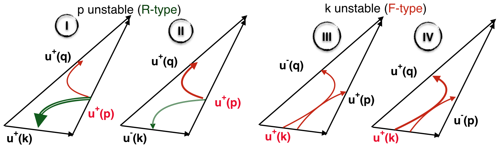
Figure 1: Schematic diagram of triadic interactions in Navier-Stokes equations. When Fourier-modes of velocity for two largest wavenumbers in a triad have the same sign of helicity, there is an inverse transfer of energy from small scales to large scales and such triads (Class-I and Class-II) are called R-type of triads. When Fourier-modes of velocity for two largest wavenumbers in a triad have the opposite sign of helicity, there is forward transfer of energy from large scales to small scales and such triads (Class-III and Class-IV) are called F-type of triads. In R-type and F-type of triads the velocity Fourier modes with medium sized wavenumber and smallest wavenumber are unstable, respectively, and transfer energy to other two Fourier modes. The arrows show direction (green double-lined for inverse and red for forward) of energy transfer.

The triads are classified as follows: Class-I contains the homochiral triads with velocity Fourier modes having same sign of helicity for all wavenumbers, i.e., $({\hat{\bm{u}}}_{\bm{k}}^{+},{\hat{\bm{u}}}_{\bm{p}}^{+},{\hat{\bm{u}}}_{\bm{q}}^{+})$; Class-II contains the triads with velocity Fourier modes having same sign of helicity for two large wavenumbers but opposite sign of helicity for two smaller wavenumbers, i.e., $({\hat{\bm{u}}}_{\bm{k}}^{+},{\hat{\bm{u}}}_{\bm{p}}^{-},{\hat{\bm{u}}}_{\bm{q}}^{-})$; Class-III contains the triads with velocity Fourier modes having same sign of helicity for the largest and the smallest wavenumbers, i.e., $({\hat{\bm{u}}}_{\bm{k}}^{+},{\hat{\bm{u}}}_{\bm{p}}^{-},{\hat{\bm{u}}}_{\bm{q}}^{+})$; and Class-IV contains triads with velocity Fourier modes having opposite sign of helicity for two larger wavenumbers but same sign of helicity for two smaller wavenumbers, i.e., $({\hat{\bm{u}}}_{\bm{k}}^{-},{\hat{\bm{u}}}_{\bm{p}}^{-},{\hat{\bm{u}}}_{\bm{q}}^{+})$.

Using linear stability analysis for energy exchange among the modes of each single triad it was argued that [32] the triads of classes I do transfer energy backward, while those of Class II, where largest wavenumbers have same sign of helicity, are capable of transferring energy from the unstable velocity Fourier mode with intermediate wavenumber to the other two modes, leading to a forward or to a backward cascade depending on the geometry of the triad [36, 37]. The triads in classes III and IV, where largest wavenumbers have opposite sign of helicity, transfer energy from the unstable velocity Fourier mode with smallest wavenumber to the other two modes with larger wavenumbers and are responsible for forward cascade of energy. However, in presence of more than one triads, competing triadic interactions do not allow simple prediction for direction of the energy transfer mechanism. Moreover depending on the actual realization of the flow based on the forcing scheme, the boundary conditions, etc., different directions of the energy transfer could be observed.

In a turbulent flow sustained by a homogeneous and isotropic forcing mechanism where all possible triadic interactions are present energy is observed to be transferred forward from large to small scales[1]. However when the dynamics is restricted to only velocity Fourier modes with one sign of helicity, i.e., interacting triads of Class-I ($s_{\bm{k}}=s_{\bm{p}}=s_{\bm{q}}$), energy cascades from small scales to the large scales [16]. This is attributed to the fact that the second quadratic invariant, Helicity, becomes sign-definite for such subset of interactions. It was also observed  [20] that presence of few percent of modes with opposite sign of helicity at all scales changes the direction of energy transfer in a singular manner; even though triads of classes II, III and IV are a small fraction of Class-I, they efficiently transfer energy to the small scales. It would therefore be important to study a system without the triads of Class-I in order to highlight their role in the dynamics of full Navier-Stokes equations.

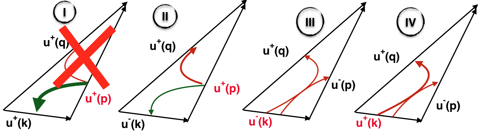
Figure 2: Schematic diagram of triadic interactions (in R2), with no triads of Class-I, i.e., all triadic interactions involving velocity Fourier modes of same sign of helicity were suppressed.

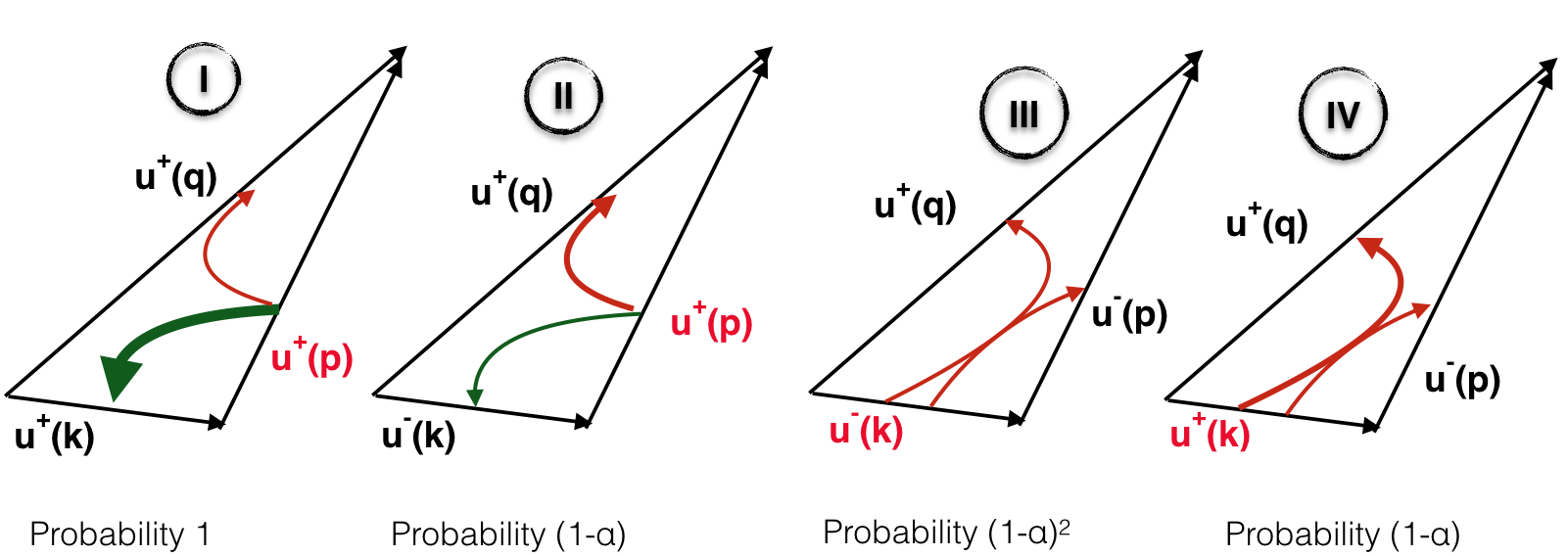
Figure 3: Schematic diagram of triadic interactions (in R3), with negative Fourier-helical modes reduced with probability of $\alpha=0.1$.

3 Direct Numerical Simulations

We have performed direct numerical simulations with a fully-dealiased, pseudo-spectral code at resolution of $512^{3}$ collocation points on a triply periodic cubic domain of size $L=2\pi$. We used a random Gaussian forcing to maintain a steady flow with

$$\langle f_{i}({\bm{k}},t)f_{j}({\bm{q}},t^{\prime})\rangle=F(k)\delta({\bm{k}}-{\bm{q}})\delta(t-t^{\prime})Q_{i,j}({\bm{k}}),$$ (15)

where $Q_{ij}({\bm{k}})$ is a projector that insures incompressibility. The amplitude $F(k)$ is nonzero only for $|k|\in[k_{\rm min}:k_{\rm max}]$. This is the standard way energy is injected at large scale in simulations of turbulent flows in order to keep homogeneity and isotropy, i.e., to keep the maximum symmetry in the system [38, 16, 20, 10, 39, 40]. Table. 1 lists the parameters of the simulations. We have used a fully helical forcing with projection on ${\bm{h}}^{+}_{\bm{k}}$ in order to ensure a maximal injection of helicity. We do not expect any dependency of small-scale statistics on the forcing adopted here because Navier-Stokes turbulence is known to have universal fluctuations in the inertial and viscous ranges [41, 42] irrespective of large-scale driving mechanism.

Table 1: Details of the Simulations. $N$: number of collocation points along each axis; $L$: size of the periodic box; $\nu$: kinematic viscosity; $k_{f}$: range of forced wavenumbers; $u_{\rm rms}$: rms velocity; $Re_{\lambda}=u_{\rm rms}\lambda/\nu$: Taylor-microscale Reynolds number, where $\lambda=\frac{2\pi}{L}\sqrt{\frac{\langle u^{2}({\bm{x}})\rangle}{\langle\left[\partial_{x}u({\bm{x}})\right]^{2}\rangle}}$ is the Taylor microscale; $\left<\varepsilon\right>$: mean energy dissipation rate; $\eta$: Kolmogorov length-scale; $T_{0}$: large-eddy-turnover time.

RUN	$N$	$L$	$\nu$	$k_{f}$	$u_{\rm rms}$	$Re_{\lambda}$	$\left<\varepsilon\right>$	$\eta$	$T_{0}$
R1	$512$	$2\pi$	$0.002$	$[1,2]$	$3.5$	$220$	$3.2$	$0.005$	$0.3$
R2	$512$	$2\pi$	$0.002$	$[1,2]$	$3.7$	$240$	$2.5$	$0.007$	$0.3$
R3	$512$	$2\pi$	$0.002$	$[1,2]$	$3.5$	$210$	$2.8$	$0.007$	$0.3$

First we carried out a simulation (R1) of standard Navier-Stokes equations with energy injected at the large scales $k_{f}\in[1,2]$. In second simulation (R2) we removed all the triads belonging to Class-I from the dynamics of the Navier-Stokes equations: we solved the following modified Navier-Stokes equations

$$\partial_{t}{\bm{u}}({\bm{x}}) +N[{\bm{u}}({\bm{x}}),{\bm{u}}({\bm{x}})]-{\cal D}^{+}N[{\bm{u}}^{+}({\bm{x}}),{\bm{u}}^{+}({\bm{x}})]$$

$$-{\cal D}^{-}N[{\bm{u}}^{-}({\bm{x}}),{\bm{u}}^{-}({\bm{x}})]=-{\bm{\nabla}}p+\nu\Delta{\bm{u}}({\bm{x}})+f^{+},$$

where $\nu$ is the viscosity and $p$ is the pressure. Such a reduction of triads preserve the conservation of energy and helicity of the system. The triads in this simulation are shown in Fig. 2. In third simulation (R3) we removed randomly $10\%$ of negatively helical velocity Fourier modes from the system using the method described in [20]. We define an operator ${D}^{\alpha}$ that projects each wavenumber with a probability $0\leq\alpha\leq 1$:

$${{\bm{u}}}^{\alpha}({\bm{x}})\equiv D^{\alpha}{{\bm{u}}}({\bm{x}})\equiv\sum_{{\bm{k}}}e^{i{\bm{k}}{\bm{x}}}\,{\mathcal{D}}^{\alpha}_{{\bm{k}}}{{\hat{\bm{u}}}_{\bm{k}}},$$ (17)

where ${\mathcal{D}}^{\alpha}_{{\bm{k}}}\equiv(1-\gamma^{\alpha}_{{\bm{k}}}){\mathbb{I}}+\gamma^{\alpha}_{{\bm{k}}}{\mathcal{P}}^{+}_{{\bm{k}}}$ and $\gamma^{\alpha}_{{\bm{k}}}=1$ with probability $\alpha$ or $\gamma^{\alpha}_{{\bm{k}}}=0$ with probability $1-\alpha$. The $\alpha$-reduced Navier-Stokes equations ($\alpha$-NSE) are

$$\partial_{t}{\bm{u}}^{\alpha}=D^{\alpha}[-{\bm{u}}^{\alpha}\cdot{\bm{\nabla}}{\bm{u}}^{\alpha}-{\bm{\nabla}}p^{\alpha}]+\nu\Delta{\bm{u}}^{\alpha},$$ (18)

Notice that the nonlinear terms on the rhs of (18) are further projected by ${D}^{\alpha}$ in order to enforce the dynamics on the selected set of modes for all times. These methods of reduction of degrees of freedom results in a loss of Lagrangian properties of the system [43]. We chose $\alpha=0.1$ for R3. The triads present in this simulation are shown in Fig. 3.

4 Results

We measured the energy flux due to the nonlinear terms, given in Eq. (12),

$${\rm\Pi}_{E}(k)=\sum_{|{\bm{k}}^{\prime}|<k}{\hat{\bm{u}}}_{\bm{k}^{\prime}}^{*}\cdot\hat{\bm{N}}_{{\bm{k}}^{\prime}},$$ (19)

across a wavenumber $k$, for all three cases. We show the total energy flux and the energy flux due to only homochiral triads (Class-I), by using either of the projected velocity modes ${\bm{u}}^{\pm}_{\bm{k}}$ in Eqs. (12) and (19) in the full Navier-Stokes equations (no mode reduction) in Fig. 4. The flux due to triads of Class-I has opposite sign to that of total flux indicating that those interactions contribute with an inverse transfer of energy already in the full equations as observed in Ref. [44]. Also in Fig. 4 we compare the total energy flux in full Navier-Stokes (from simulation R1), in $\alpha$-reduced Navier-Stokes (R3) and in Navier-Stokes without the triads of Class-I (from simulation R2); there is no significant difference in the total flux. This is due to the fact that the net total flux has strictly zero backward energy transfer for all the three cases.

Figure 4: Semi-log plots of energy fluxes. Flux of energy due to triads formed by three Fourier modes with same sign of helicity (Class-I) in full Navier-Stokes equations (R1) are shown by filled squares whereas the total flux of energy is shown by empty squares. Total energy flux from simulation (R3) with $\alpha=0.1$ are shown by circles whereas triangles show the same from simulation (R2) of Navier-Stokes equations without triads of Class-I.

In Fig. 5 we compare the energy spectra for the same three cases (R1, R2 and R3) which are indistinguishable from each other. Energy spectra are not sensitive to reduction of triads as long as triads facilitating forward energy cascade are present in the system. This is in agreement with earlier observation  [20].

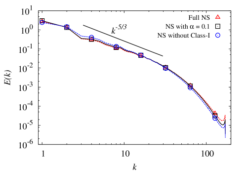
Figure 5: Log-log plots of energy spectra. Triangles, squares and circles show the spectra of energy from simulations of full Navier-Stokes equations (R1), $\alpha$-reduced Navier-Stokes equations (R3) and Navier-Stokes equations without Class-I triads (R2), respectively. The black line shows $k^{-5/3}$ scaling for reference.

One goal of this paper is to study the effects of removing Class-I triads on the intermittency of the system. We measured the flatness, defined as

$$F(r)=\frac{S_{4}(r)}{[S_{2}(r)]^{2}},$$ (20)

and hyperflatness, defined as

$$H(r)=\frac{S_{6}(r)}{[S_{2}(r)]^{3}},$$ (21)

of longitudinal velocity increments

$$\delta_{r}u_{L}=[{\bm{u}}({\bm{x}}+{\bm{r}})-{\bm{u}}({\bm{x}})]\cdot\frac{{\bm{r}}}{r},$$ (22)

and transverse velocity increments

$$\delta_{r}u_{T}=[{\bm{u}}({\bm{x}}+{\bm{r}})-{\bm{u}}({\bm{x}})]\cdot\frac{\bf r^{\prime}}{r^{\prime}},$$ (23)

where ${\bf r^{\prime}}$ is perpendicular to the direction of ${\bm{r}}$, shown in Fig. 6 for three cases R1-R3. Structure functions, longitudinal and transverse, of order $p$ are defined as

$$S_{p}^{L,T}(r)=\left<(\delta_{r}u_{L,T})^{p}\right>,$$ (24)

where angular brackets denote spatial average.

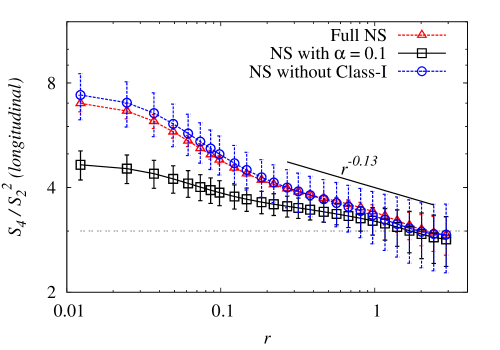
(a) (b)

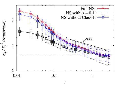
Figure 6: (a) Flatness of longitudinal velocity increments from simulations of full Navier-Stokes equations (R1), $\alpha$-reduced Navier-Stokes equations (R3) and Navier-Stokes equations without Class-I triads (R2) are shown by triangles, squares and circles, respectively. (b) Flatness of transverse velocity increments. Error-bars show the fluctuations in the steady-state.

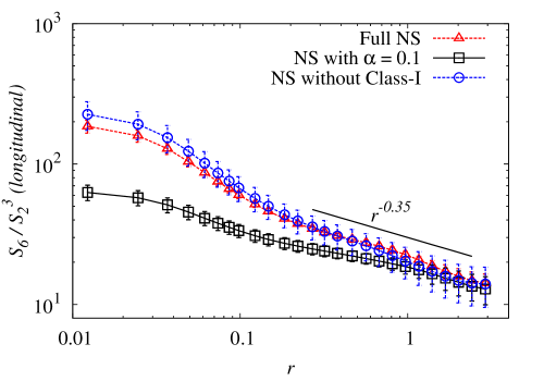
(a) (b)

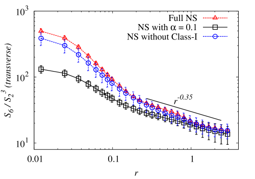
Figure 7: (a) Hyperflatness of longitudinal velocity increments from simulations of full Navier-Stokes equations (R1), $\alpha$-reduced Navier-Stokes equations (R3) and Navier-Stokes equations without Class-I triads (R2) are shown by triangles, squares and circles, respectively. (b) Hyperflatness of transverse velocity increments. Error-bars show the fluctuations in the steady-state.

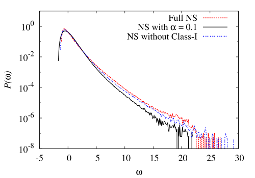
(a) (b)

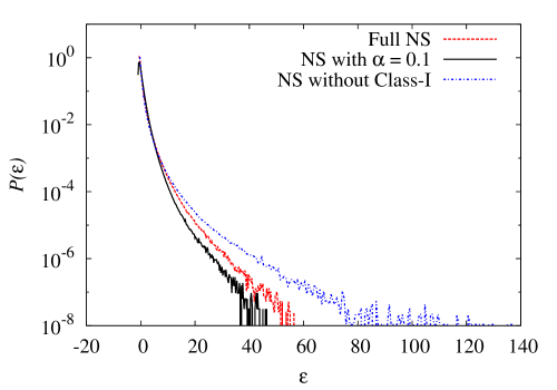
Figure 8: (a) Plots of probability distribution function (pdf) of $\omega$, where $\omega^{2}=|\nabla\times{\bm{u}}|^{2}$ is the enstrophy, from simulations of full Navier-Stokes equations (R1), $\alpha$-reduced Navier-Stokes equations (R3) and Navier-Stokes equations without Class-I triads (R2) are shown by triangles, squares and circles, respectively. (b) Plots of pdf of local energy dissipation rates $\varepsilon=2\nu(\sum_{i,j}\partial_{i}u_{j}-\partial_{j}u_{i})^{2}$.

The Flatness of both longitudinal and transverse velocity increments in the inertial range, for the full Navier-Stokes (R1) and the Navier-Stokes with only heterochiral triads (R2) are comparable within the error-bars (See Fig. 6a). This indicates that homochiral (Class-I) triads, which are responsible for inverse energy transfer, have no significant role in intermittency in the inertial range of scales. However the flatness for the $\alpha$-reduced Navier-Stokes equations (R3) is much lower than the full Navier-Stokes equations (R1). A similar behaviour is also observed for the longitudinal and transverse hyper-flatness which are shown in Fig. 7. It is also observed that in absence of homochiral triads (R2) the intensity of the longitudinal flatness at the gradient scale is marginally higher than the full Navier-Stokes case (R1) and the opposite is measured for the transverse increments, which could be an indication that the presence/absence of homochiral triads slightly modifies the small-scale vortical structure of the flow.

To further investigate this aspect, we measured the probability distribution function (pdf) of local energy dissipation rate and of local enstrophy (see Fig. 8). As inferred from the measurement of the flatness we observed that the pdf of energy dissipation has a longer tail for the case of only heterochiral triads and the opposite happens for the enstrophy distribution, confirming that the absence of homochiral triads might have a different impact in regions of high strain or high rotation.

Visualisation of the flow field with plots of isovorticity surfaces are shown in Fig. 9. In both cases where we have removed the Class-I triads or a fraction of triads of classes other than Class-I the filament-like structures are reduced. In absence of Class-I triads we observe more sheet-like structures. The visible change in the ‘coherency’ of the flow together with the intermittency robustness as a function of the removal of Class-I triads suggest that the main signature of anomalous scaling in the inertial range of the full Navier-Stokes equations is not strongly connected to any clearly detectable ‘coherent structure’.

Figure 9: Isovorticity surfaces for (a) Full Navier-Stokes (R1), (b) $\alpha$-reduced Navier-Stokes with $\alpha=0.1$ (R3) and (c) Navier-Stokes without the Class-I triads (R2). The isovalues of the vorticity is three standard deviations above the mean value. The color code correspond to the value of helicity: from high positive values (red) to high negative values (blue).

5 Conclusions

We carried out direct numerical simulations of 3D Navier-Stokes equations and of the Navier-Stokes equations without the triads formed by homochiral velocity Fourier modes (here taken the positive ones). We observed that inertial range intermittency remains almost unaffected confirming that the forward energy cascade is mainly dominated by heterochiral triads. On the other hand, by removing negative helical modes also on the heterochiral triads, intermittency strongly reduces, suggesting that the formation of small-scale intense events needs almost all triads that transfer energy forward. A small change at the scale crossing between viscous and inertial terms is observed when homochiral triads are removed from the dynamics in agreement with the presence of more sheet-like structures in the flow. It would be interesting to extend this kind of studies to less symmetric flow configuration. In particular it might be key to apply it for the case of turbulence under rotation, where previous works have shown that helicity plays a role in enhancing the inverse energy cascade regime [45]. On the other hand, rotating turbulence tends to become quasi-2D in the limit of very intense rotation rate [11, 46] , and therefore there must exists a trade-off between the role played by helicity (exactly vanishing in 2D) and rotation [47]. Similarly, it is not known the role played by homochiral and heterochiral triads in strongly anisotropic flows as for the case of homogeneous shear and for decaying turbulence. Work in this direction is ongoing and it will be reported elsewhere.

6 Acknowledgement

We acknowledge funding from the European Research Council under the European Union’s Seventh Framework Programme, ERC Grant Agreement No 339032 and support from COST Action MP1305. GS acknowledges support from Atmospheric Mathematics (AtMath) collaboration at University of Helsinki.

References

References

- [1] U. Frisch, Turbulence: the legacy of A.N. Kolmogorov (Cambridge University Press, Cambridge, UK,1995).
- [2] A. N. Kolmogorov Dokl. Akad. Nauk. SSSR 32, 19 (1941).
- [3] G. Boffetta and S. Musacchio, Phys. Rev. E 82, 016307 (2010).
- [4] R. H. Kraichnan, Phys. Fluids 10, 1417 (1967).
- [5] P. D. Mininni, A. Alexakis, and A. Pouquet, Phys. Fluids 21, 015108 (2009).
- [6] E. Deusebio and E. Lindborg, J. Fluid Mech. 755, 654 (2014).
- [7] A. Celani, S. Musacchio, and D. Vincenzi, Phys. Rev. Lett. 104, 184506 (2010).
- [8] A. Brandenburg, Astrophysical J. 550, 824 (2001).
- [9] D. Lohse and K. Q. Xia, Annu. Rev. Fluid Mech. 42, 335 (2010).
- [10] G. Sahoo, A. Alexakis, and L. Biferale, Phys. Rev. Lett. 118, 164501 (2017).
- [11] L. Biferale, F. Bonaccorso, I.M. Mazzitelli, M.A.T. van Hinsberg, A.S. Lanotte, S. Musacchio, P. Perlekar, and F. Toschi, Phys. Rev. X 6, 041036 (2016).
- [12] P. F. Embid and A. J. Majda, Geophys. Astrophys. Fluid Dynamics 87, 1-50 (1998).
- [13] J. Sukhatme and L. M. Smith, Geophys. Astrophys. Fluid Dynamics 102, 437-455 (2008).
- [14] H. K. Moffatt, J. Fluid Mech. 35, 117 (1969).
- [15] H. K. Moffatt and A. Tsinober, Annu. Rev. Fluid Mech. 24, 281 (1992).
- [16] L. Biferale, S. Musacchio, and F. Toschi, Phys. Rev. Lett. 108, 164501 (2012).
- [17] L. Biferale, S. Musacchio, and F. Toschi, J. Fluid Mech. 730, 309 (2013).
- [18] P. Constantin, A. Majda, Commun. Math. Phys. 115, 435 (1988).
- [19] L. Biferale and E. S. Titi, J. Stat. Phys. 151, 1089 (2013).
- [20] G. Sahoo, F. Bonaccorsso, and L. Biferale, Phys. Rev. E 92, 051002 (2015).
- [21] G. Sahoo and L. Biferale, Eur. Phys. J. E 38, 114 (2015).
- [22] A. Brissaud, U. Frisch, J. Leorat, M. Lesieur, and M. Mazure, Phys. Fluids 16, 1366 (1973).
- [23] C.E. Laing, R. L. Ricca, and D. W. L. Summers, Scientific Reports 5, 9224 (2015). nonlocal.
- [24] P. D. Ditlevsen, Phys. Fluids 9, 1482 (1997).
- [25] R. Stepanov, E. Golbraikh, P. Frick, and A. Shestakov, Phys. Rev. Lett. 115, 234501 (2015).
- [26] D. Biskamp, Magnetohydrodynamic Turbulence (Cambridge University Press, Cambridge, UK, 2003).
- [27] D.D. Holm, R.M. Kerr, Phys. Fluids 19, 025101 (2007).
- [28] J. Baerenzung, H. Politano, Y. Ponty, A. Pouquet, Phys. Rev. E 77, 046303 (2008)
- [29] R. Benzi, L. Biferale, R. M. Kerr, and E. Trovatore, Phys. Rev. E 53, 3541 (1996).
- [30] Q. Chen, S. Chen, and G. L. Eyink, Phys. Fluids 15, 361 (2003);
- [31] Q. Chen, S. Chen, G. L. Eyink, and D. D. Holm, Phys. Rev. Lett. 90, 214503 (2003).
- [32] F. Waleffe, Phys Fluids A 4, 350 (1992).
- [33] C. Herbert, Phys. Rev. E 89, 013010 (2014).
- [34] R. H. Kraichnan, J. Fluid Mech. 47, 525 (1971).
- [35] L. M. Smith and Y. Lee, J. Fluid Mech. 535, 111 (2005).
- [36] M. De Pietro, L. Biferale, and A. A. Mailybaev, Phys. Rev. E 92, 043021 (2015).
- [37] N. M. Rathmann and P. D. Ditlevsen, Phys. Rev. E 94, 033115 (2016).
- [38] L. M. Smith, F. Waleffe, Phys. Fluids 11, 1608 (1999).
- [39] V. Borue and S. A. Orszag, Europhys. Lett. 29, 687 (1995).
- [40] K. Alvelius, Phys. Fluids 11, 1880 (1999).
- [41] J. Schumacher, J. D. Scheel, D. Krasnov, D. A. Donzis, V. Yakhot, and K. R. Sreenivasan, Proc. Natl. Acad. Sci. 111, 10961 (2014).
- [42] R. Benzi, L. Biferale, R. Fisher, D.Q. Lamb and F. Toschi, J. Fluid Mech. 653, 221 (2010).
- [43] H. K. Moffatt, J. Fluid Mech. 741, R3 (2014).
- [44] A Alexakis, J. Fluid Mech 812, 752 (2017).
- [45] A. Pouquet and P. D. Mininni, Phil. Trans. R. Soc. A 368, 1635–1662 (2010).
- [46] S. Chakraborty, Europhys. Lett.79, 14002 (2007).
- [47] L. Biferale, M. Buzzicotti and M. Linkmann, Phys. Fluids 29, 111101 (2017).