Study of spin models with polyhedral symmetry on square lattice

Abstract

Anisotropy is important for the existence of true long range order in two dimensional (2D) systems. This is firmly exemplified by the $q$-state clock models in which discreteness drives the quasi-long range order into a true long range order at low temperature for $q>4$. Previously we studied 2D edge-cubic spin model, which is one of the discrete counterpart of the continuous Heisenberg model, and observed two finite temperature phase transitions, each corresponds to the breakdown of octahedral ($O_{h}$) symmetry and $C_{3h}$ symmetry, which finally freezes into ground state configuration. The present study investigates discret models with polyhedral symmetry, obtained by e equally partioning the $4\pi$ of the solid angle of a sphere. There are five types of models if spins are only allowed to point to the vertices of the polyhedral structures such as Tetrahedron, Octahedron, Hexahedron, Icosahedron and Dodecahedron. By using Monte Carlo simulation with cluster algorithm we calculate order parameters and estimate the critical temperatures exponents of each model. We found a systematic decrease in critical temperatures as the number of spin states increases (from the Tetrahedral to Dodecahedral spin model).

I Introduction

Phase transitions are ubiquitious phenomena in nature, firmly exemplified by the melting of ice, spontaneous magnetization of ferromagnetic material and transformation from normal conductor of metal into a superconductivity at very low temperatures. In general, a phase transition is related to the breakdown of symmetry of a systemLandau . For a thermal-driven phase transition, systems are in high degree of symmetry at high temperature because all configurational spaces are accessible. The decrease in temperature will reduce thermal fluctuation and the system stays in some favorable states. If the phase transition occurs with no latent heat, the system experiences continuous transition, also known as second order phase transition, which is a transition between the ordered and the disordered state.

According to Mermin-Wagner-Hohenberg theorem, spin models with continuous symmetry and short-range interaction can not have a true long range order (TLRO) for two dimensional (2D) lattices, thus no finite temperature transitionMermin . However, a unique type transition called Kosterlitz-Thouless (KT) transition can exist in the XY model (O(2) symmetry)kosterlitz . It is a transition between a high temperature paramagnetic phase and a low-temperature quasi-long range order (QLRO), known as KT phase. If the $2\pi$ planar angle of the XY model is discretized into $q$ equal angles, we obtain a $q$-state Clock model. This model, apart from inheriting the KT phase, possesses a lower-temperature TLRO driven by the discretnessjose ; ts04 .

It is of interest to systematically study the role played by the discrete symmetry for 3D case. In analogy with the Clock models for 2D symmetry, we discretize the continuous orientation of Heisenberg spin (O(3) symmetry) for obtaining spin models with polyhedral symmetry. This is done by equally partioning the $4\pi$ solid angle of a sphere, resulting in five regular polyhedrons, also known as Platonic solids, i.e., Tetrahedron, Octahedron, Cube, Icosahedron and DodecahedronMacLean . Table 1 tabulates the characteristics of each structure, to which we define a model with spin orientations restricted to point to the vertices of the corresponding structure. Previously we study the edge-cubic spin model with underlying symmetry, the Octahedral symmetry ($O_{h}$), similar to that of Hexahedron and Octahedron (cubic) modelts06. However, spin orientation of the model is only allowed to point to the middle point of cubic’s edges, therefore there are 12 possible states. We observed two finite temperature phase transitions which comes from the fact that this model partitions the solid angle unequally.

The present paper studies models with polyhedral symmetry. We expect to observe finite temperature second order phase transitions due to the discreteness.

Table 1: Characteristics of regular polyhedrons.

Name	Vertices	Faces	Edges	Group Symmetry
	($q$-state)
Tetrahedron	4	4	6	$S_{4}$
Octahedron	6	8	12	$O_{h}=S_{4}\times C_{2}$
Hexahedron (cube)	8	6	12	$O_{h}$
icosahedron	12	20	30	$A_{5}\times C_{2}$
dodecahedron	20	12	30	$A_{5}\times C_{2}$

The remaining part of the paper is organized as follows: Section II describe the model and the method. The result is discussed in Section III. Section IV is devoted to the summary and concluding remark.

II Model and Simulation Method

The polyhedral spin models are the discrete version of the Heisenberg model with spins are only allowed to point to the vertices of the structures listed in Table 1. The Hamiltonian of the model is written as follows

$$H=-J\sum_{\langle ij\rangle}\vec{s}_{i}\cdot\vec{s}_{j}$$ (1)

where $\vec{s}_{i}$ is the spin on site $i$-th. Summation is performed over all the nearest-neighbor pairs of spins on a square lattice with ferromagnetic interaction ($J>0$) and with periodic boundary condition. The energy of the ground state configuration, i.e., when all spins having a common orientation, is $-2NJ$ with $N$ is the number of spins.

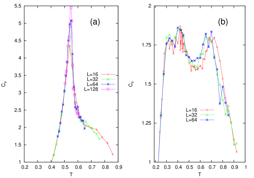
Figure 1: The temperature dependence of the specific heat for various system sizes of (a) Dodecahedron and Icosahedron models. As shown, there exists a clear peak for Icosahedron while two peaks for dodecahedron. The peaks may signify the existence of phase transitions. The error bar, in average, is in the order of symbol size.

We use the canonical Monte Carlo (MC) method with single cluster spin updates introduced by Wolff wolff and adopt Wolff’s idea of embedded scheme in constructing a cluster for the 3D vector spins. Spins are projected into a randomly generated plane so that they are divided into two Ising-like spin groups. This scheme is essential for carrying out cluster algorithm applied to such spins as 2D and 3D continuous spins.

After the projection, the usual steps of the cluster algorithm is performed kasteleyn , i.e., by connecting bonds from the randomly chosen spin to its nearest neighbors of similar group, with suitable probability. This procedure is repeated for neighboring spins connected to a chosen spin until no more spins to include. One Monte Carlo step (MCS) is defined as visiting once the whole spins randomly and perform cluster spin update in each visit. It is to be noticed that for each step a spin may be updated many times, in average, in particular near the critical point.

Measurement is performed after enough equilibration MCS’s ($10^{4}$ MCS’s). Each data point is obtained from the average over several parallel runs, each run is of $4\times 10^{4}$ MCS’s. To evaluate the statistical error each run is treated as a single measurement. For the accuracy in the estimate of critical exponents and temperatures, data are collected upto more than 100 measurements for each system size.

III Results and Discussion

III.1 Specific heat and magnetization

The first step in the search for any possible phase transition is to measure the specific heat defined as follows

$$C_{v}(T)=\frac{1}{Nk_{B}T^{2}}(\langle E^{2}\rangle-\langle E\rangle^{2})$$ (2)

where $E$ is the energy in unit of $J$ while $\langle\cdots\rangle$ represents the ensemble average of the corresponding quantity. All temperatures are expressed in unit of $J/k_{B}$ where $k_{B}$ is the Boltzmann constant.

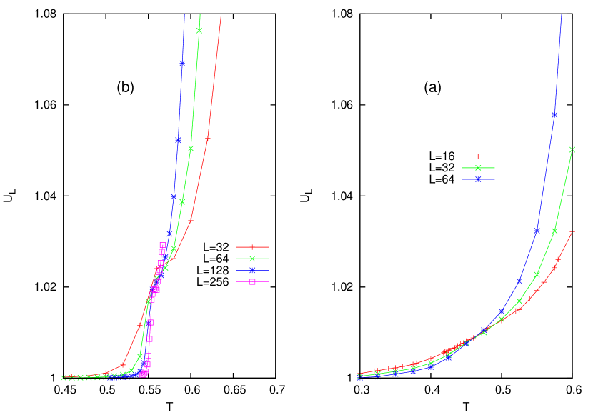
Figure 2: Temperature dependence of moment ratios for several system sizes of (a) Icosahedron and (b) Dodecahedron models. The crossing points indicates a phase transition between the disordered and the intermediate phase. Error bar is in the order smaller than the symbol size.

The specific heats of Dodecahedron and Icosahedron models are ploted in Fig. 1. Although peaks in a specific heat are more directly related to energy fluctuation, they may signify the existence of phase transitions. More quantitative analysis in searching for phase transition is performed through the evaluation of the order parameters from which critical temperatures and exponents may be extracted using finite size scaling (FSS) procedure. In this paper we present the analysis of obtaining exponents only for Dodecahedron and Icosahedron models as other models are equivalent to the commonly known models. The Tetrahedron model is equivalent to the 4-state Potts model while the Hexahedron (corner-cubic model) is equivalent to the Ising model. The Octahedron model which is face-cubic model has been studied by Yasuda and Okabeyasuda .

As the probed system is ferromagnetic we consider magnetization $M=|\sum\vec{s}_{i}|$ as the order parameter. By defining $M^{k}$ as the $k$-th order moment of magnetization and $g(R)=\sum\vec{s}(r)\cdot\vec{s}(r+R)$ as correlation function, the moment and correlation ratios are respectively written as follows

$$U_{L} = \frac{\langle M^{4}\rangle}{\langle M^{2}\rangle^{2}}$$ (3)

$$Q_{L} = \frac{\langle g(L/2)\rangle}{\langle g(L/4)\rangle}$$ (4)

Precisely, the distance $R$ for the correlation function $g(R)$ is a vector quantity. Here we take the simple and more convenient distances, i.e., $L/2$ and $L/4$, both in $x$- and $y$-directions.

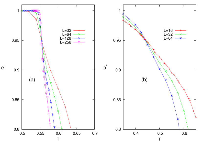
Figure 3: Temperature dependence of correlation ratios for several system sizes of (a) Icosahedron and (b) Dodecahedron models. The absis of the crossing points are the critical temperatures of the corresponding models, comparable to the numerical values given by the moment ratio of Fig. 2. Error bar is in the order smaller than the symbol size.

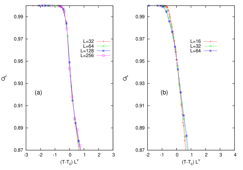
Figure 4: The FSS plot of correlation ratio for (a) Icosahedorn and (b) Dodecahedron models. The estimates of critical temperature and the exponent of correlation length $\nu$ are obtained.

The existence of a phase transition can be observed from the temperature dependence of $U_{L}$ and $Q_{L}$. At very low temperature where system is approaching the ground state, both moment and correlation ratio are trivial. Due to the absence of fluctuation, the distribution of $M$ is a delta-like function, giving moment ratio equals to unity. Correlation ratio also goes to unity as correlation function for small and large distance is the same due to highly correlated state. In excited states, the moment and the correlation ratios are not trivial, they depend on temperature. The plot of moment ratio for various system sizes of Icosahedron and Dodecahedron models shown in Fig. 2, exhibits crossing points indicating phase transitions. The crossing point for the Icosahedron model is slightly mild compared to the that of Dodecahedron which is related to the performance of moment ratio. Crossing points for both models are strongly indicated by the plot of correlation ratio shown in Fig. 3. The procedure for estimating critical temperatures using FSS will be presented in the next subsection.

III.2 Finite Size Scaling

FSS analysis for obtaining critical temperature and exponents are shown in Fig. 4, where we plot correlation ratio of the models. In general, moment ratio has larger correction to scaling than the correlation ratio tomita02a ; tasrief05 , which happens to be the case here, shown for example by the mild crossing point of moment ratio for Icosahedron models (Fig. 2a), while sharp crossing for correlation ratio (Fig. 2b). However, if the variables of the two correlation functions are not local quantity, the correlation ratio may have larger correction to scaling. Our estimate of $T_{c}$ is based on result obtained from the correlation ratio. For Icosahedron model, the estimated values of $T_{c}$ and $\nu$ are respectively 0.555(1) and 1.30(1), while for Dedecahedron, $T_{c}=0.438(1)$ and $\nu=2.01(1)$. The number in bracket is the uncertainty in the last digit.

Using the correlation ratio we can also extract the decay exponent $\eta$ of the correlation function. This is done by looking at the constant value of correlation ratio $Q$ for different sizes and then find the corresponding correlation function $g(L/2)$. The correlation function is in power-law dependence on the system size, $g(L/2)\sim L^{-\eta}$ tomita02a . Therefore, if we plot $g(L/2)$ versus $L$ for various $Q$’s in logarithmic scale, as in Fig. 5, the value of $\eta$ will correspond to the gradient of the best-fitted line for each constant of correlation ratio. There are several lines plotted in Fig. 5. Since the critical temperature is associated with the value of $Q\sim 0.95$ for Icosahedron model (Fig. 3(a)), we assign $\eta=0.199(1)$ as the best estimate. For the Dodecahedron model (Fig. 5b) the estimate in $\eta=0.149(1)$.

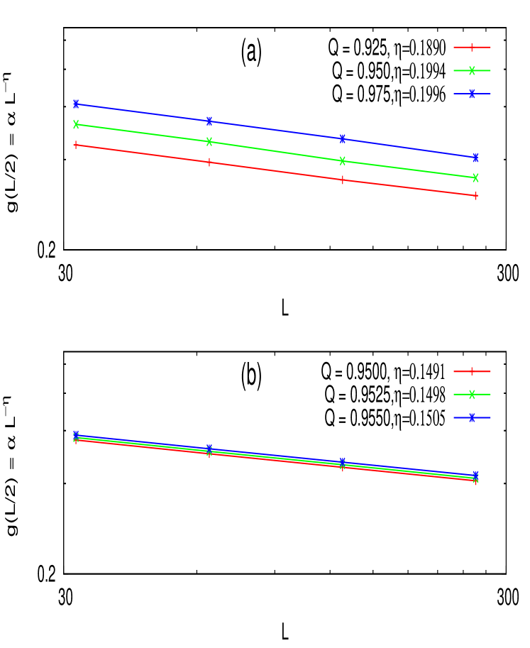
Figure 5: Double logarithmic plot of $\bar{g}(L/2)$ vs $L$. The gradient of the fitted line associated with $Q=0.82$ for Icosahedron and $Q=0.92$ for Dodecahedron model. The best estimate for $\eta$ are respectively $0.149(1)$ and $0.199(1)$.

After obtaining the critical exponents, we can now discuss the universality classes of the existing phase transitions. The expectation that models with the same underlying symmetry has to belong to the same universality class seems to be too good to apply. As indicated, although the underlying symmetry of the Icosahedorn and the Dodecahedron is the same, both models have different universality class. It is of interest to investigata whether this finding also holds for 3D systems.

IV Summary and Concluding Remarks

In summary, we have studied critical properties of spin models with polyhedral symmetry on a square lattice. They are the discrete version of the Heisenberg model. If the $4\pi$ solid angle is equally partitioned, then there exist five regular octahedrons, as listed in Table 2. We only consider the Icosahedron and the Dodecahedron models as the Tetrahdron and the octahedron are equivalent to the common models, i.e., the Ising and the 4-state Potts model, respectively while the Hexahedron model has been studied by Yasuda and Okabe. We observed a second order phase transition for each correspoding model studied and estimated the critical temperature and exponents by using FSS of correlation ratio. Our results are tabulated in Table 2, including results from previous studies. We found a systematic decrease in critical temperatures as the number of spin states increases ($q\to\infty$ as $T_{c}\to 0$). This implies that $T_{c}=0$ for the model with continuous symmetry, which emphasizes the importance of discretness in 2D systems.

Table 2: Critical temperatures and exponents of phase transitions of 2D Polyhedral spin models.

Model	$T_{c}$	$\nu$	$\eta$
($q$-state)
4	$(4/3)*(1/\ln(3))=0.214$	2/3	1/4
6	$0.9085(2)$	0.685(2)	0.23(1)
8	$(1/3)*(2/\ln(2.42))=0.756$	1	1/4
12	$T_{c}=0.555(2)$	$\nu=1.31(1)$	0.199(1)
20	$T_{c}=0.438(1)$	$\nu=2.0(1)$	0.149(1)
12∗ts08	$0.602(1)$	1.50(1)	0.260(1)

References

- (1) L. D. Landau, On the theory of phase transition, in Collected Paper of L. D. Landau, edited by D. T. Haar (Pergamon Press, 1965).
- (2) N. D. Mermin and H. Wagner, Phys. Rev. Lett. 17 1133, (1966) ; P. C. Hohenberg, Phys. Rev. 158, 383 (1967).
- (3) J. M. Kosterlitz and D. Thouless, J. Phys. C 6, 1181 (1973); J. M. Kosterlitz, J. Phys. C 7, 1046 (1974).
- (4) K. J. M. MacLean, A Geometric Analysis of the Platonic Solids and Other Semi-Regular Polyhedra , (The Big Pictures. Press, Oxford, 2002).
- (5) J. V. José, L. P. Kadanoff, S. Kirkpatrick, and D. R. Nelson, Phys. Rev. B 16, 1217 (1977).
- (6) T. Surungan, Y. Okabe, and Y. Tomita, J. Phys. A 37, 4219 (2004).
- (7) Tasrief Surungan, Naoki Kawashima and Yutaka Okabe, Phys. Rev. B77, 214401 (2008).
- (8) A. Aharony, Phys. Rev. B 10, 3006 (1974).
- (9) D. Kim, P. M. Levy and L. F. Uffer, Phys. Rev. B 12, 989 (1975).
- (10) J. Sznajd and M. Dudziński, Phys. Rev. B 59, 4176 (1999).
- (11) P. Calabrese and A. Celi, Phys. Rev. B 66, 184410 (2002).
- (12) J. M. Carmona, A. Pelissetto, and E. Vicari, Phys. Rev. B 61, 15136 (2000).
- (13) P. Calabrese, E. V. Orlov, D. V. Pakhnin and A. I. Sokolov, Phys. Rev. B 70, 094425 (2004).
- (14) T. Yasuda and Y. Okabe, in preparation.
- (15) J. Ashkin and E. Teller, Phys. Rev. 64, 178 (1943).
- (16) U. Wolff, Phys. Rev. Lett. 62, 361 (1989).
- (17) P. W. Kasteleyn and C. M. Fortuin, J. Phys. Soc. Jpn, Suppl. 26, 11 (1969); C. M. Fortuin and P. W. Kasteleyn, Physica (Amsterdam) 57, 536, (1972).
- (18) Y. Tomita and Y. Okabe, Phys. Rev. B 66, 180401(R) (2002).
- (19) T. Surungan and Y. Okabe, Phys. Rev. B71, 188428 (2005).
- (20) F. Y. Wu, Rev. Mod. Phys. 54, 235, (1982).