On the emergence of the ${\bf\Lambda}$CDM model from self-interacting Brans-Dicke theory in ${\bf d=5}$

Abstract

We investigate whether a self-interacting Brans-Dicke theory in $d=5$ without matter and with a time-dependent metric can describe, after dimensional reduction to $d=4$, the FLRW model with accelerated expansion and non-relativistic matter. By rewriting the effective 4-dimensional theory as an autonomous three-dimensional dynamical system and studying its critical points, we show that the $\Lambda$CDM cosmology cannot emerge from such a model. This result suggests that a richer structure in $d=5$ may be needed to obtain the accelerated expansion as well as the matter content of the 4-dimensional universe.

1 Introduction

Several observations (such as SNe Ia, baryon acoustic oscillations, and the cosmic microwave background, see for instance Alves2016 ) indicate that the universe is currently undergoing an accelerated expansion. In the framework of the Standard Cosmological Model, such an expansion is only possible if matter with unusual properties is added as a source of Einstein’s Equations (EE) Frieman2008 . The simplest candidate is the cosmological constant, but there is a huge discrepancy between its theoretical value and the one that follows from observations Carroll2003 . Models with scalar or vector fields (see Li2011 for a review of these and other candidates) have also been considered to describe what is known as dark energy. Since none of these proposals is free of problems, several alternatives that avoid the introduction of dark energy have been investigated. Among them we can mention theories of gravity that go beyond General Relativity Clifton2011 and inhomogeneous cosmological models Bolejko2016 . Yet another interesting proposal is based on the hypothesis that the dimensionality of the universe is actually greater than four. The common theme in the many realizations of this idea is that an effective energy-momentum tensor of purely geometrical origin, generated by the reduction of some theory of gravitation defined in $d>4$ to $d=4$, is used to generate the accelerated expansion and/or ordinary matter.

In particular, the reduction of gravitational theories from $d=5$ to $d=4$ has been repeatedly explored in the literature Wesson2006 . An appealing example of this type was presented in Wesson1992 , where the energy-momentum of ordinary matter in $d=4$ arises from the extra-dimensional sector of the theory defined by $G_{AB}=0$.

More generally, theories in which the matter content in $d=4$ is induced by dimensional reduction of the vacuum equations of a gravitational theory defined in $d=5$ are generically known today as Induced Matter Theories (IMT) Wesson2006 . They have been extended in several directions, such as Brans-Dicke (BD) theory PoncedeLeon2009 ; Reyes2009 ; PoncedeLeon2010 ; Bahrehbakhsh2010 ; Rasouli2011 ; Rasouli2016 , $f(R)$ theories Borzou2009 ; Troisi2017 , and $f(R,T)$ theories Moraes2015 . Here we shall investigate the possibility of describing the accelerated expansion of the 4-dimensional universe as well as ordinary matter starting from BD theory in the presence of a potential in $d=5$. Cosmological evolution in self-interacting BD theory has been studied both in $d=4$ (see for instance Santos1997 ; Sen2003 ; Chakra2009 ) and in $d=5$ Periv2003 . We shall show that in an appropriate cosmological setting, the $d=5$ self-interacting BD theory is equivalent to a self-interacting BD theory in $d=4$ plus an extra scalar field (associated to the time-dependence of the metric coefficient of the fifth dimension), which is suitable for the application of dynamical analysis methods. In particular, by imposing that the critical points of the dynamical system are deSitter-like, it is possible to determine whether the effective model in $d=4$ can describe the accelerated expansion as well as the matter content of the 4-dimensional universe.

The paper is organized as follows. In Sec. 2, we obtain the effective theory in $d=4$ starting from a BD theory in vacuum in $d=5$ and in the presence of a potential. In Sec. 3, we write the field equations in $d=4$ as an autonomous three-dimensional dynamical system, and obtain its critical points, under the assumption that $\dot{H}=0$. We pay special attention to the eigenvalues of the linearization matrix associated to each critical point, and search for ranges of the parameters of the model such that the critical point is a stable one. We close with some comments in Sec. 4.

2 Brans-Dicke Theory in ${\bf d=5}$ and its reduction to ${\bf d=4}$

Our starting point is BD theory of gravity in five dimensions, with the action in the Jordan frame given by

$$^{(5)}\!{\cal S}=\frac{1}{2\kappa_{5}}\int{d^{5}y\sqrt{{}^{(5)}\gamma}\left[\phi\,^{(5)}\!R-\frac{\omega}{\phi}\gamma^{AB}\nabla_{\!A}\phi\nabla_{\!B}\phi-2V(\phi)\right]},$$ (1)

where ${}^{(5)}\!\gamma$, is the determinant of the 5-dimensional metric $\gamma_{AB}$, $\phi$ is the BD scalar field directly coupled to the 5-dimensional Ricci scalar ${}^{(5)}\!R$, $\nabla_{\!A}$ is the covariant derivative in $d=5$, $\omega$ is the BD parameter and $V(\phi)$ is the scalar field potential. The variation of the action wrt $\gamma_{AB}$ yields

$${}^{(5)\>}\!G_{AB} =\kappa_{5}\,^{(5)}T_{AB}+\frac{\omega}{\phi^{2}}\left[\nabla\!_{A}\,\phi\nabla\!_{B}\,\phi-\frac{\gamma_{AB}}{2}\nabla^{C}\phi\nabla\!_{C}\,\phi\right]+$$ (2)

$$+\frac{1}{\phi}\left[\nabla_{A}\nabla_{B}\phi-\gamma_{AB}\,^{(5)}\Box\phi\right]-\frac{V(\phi)}{\phi}\gamma_{AB},$$

where

${}^{(5)}\Box=\nabla^{A}\nabla\!_{A}$, and ${}^{(5)\>}\!G_{AB}$ is the Einstein tensor in $d=5$, given by ${}^{(5)\>}\!G_{AB}=\,^{(5)}\!R_{AB}-\frac{1}{2}\gamma_{AB}\,^{(5)}\!R$.

Variation of the action given in Eqn.(1) wrt $\phi$ results in

$$\frac{2\omega}{\phi}\,^{(5)}\Box\phi-\frac{\omega}{\phi^{2}}\nabla^{C}\phi\nabla\!_{C}\,\phi+\,^{(5)}\!R-2{V^{\prime}(\phi)}=0,$$ (3)

where the prime $(\prime)$ denotes derivative with respect to $\phi$. Taking the trace of Eqn.(2) we find

$$^{(5)}\!R=\frac{\omega}{\phi^{2}}\nabla^{C}\phi\nabla\!_{C}\,\phi+\frac{8}{3}\frac{{}^{(5)}\Box\phi}{\phi}+\frac{10}{3}\frac{V(\phi)}{\phi},$$ (4)

which, when substituted in (3) yields

$$^{(5)}\Box\phi=-\frac{5V(\phi)}{3\omega+4}+\frac{3V^{\prime}(\phi)}{3\omega+4}.$$ (5)

We shall show next how Eqns.(2) and (5) are reduced to $d=4$ in a particular cosmological setting, giving as a result the usual BD theory with the addition of an extra scalar field, whose dynamics and coupling to $\phi$ are determined by the reduction.

In the coordinate chart $\left\{y^{A}\right\}=\left\{x^{\mu},z\right\}$ we consider the 5D line element

$$ds_{{}_{5}}^{2}=\gamma_{AB}dy^{A}dy^{B}=dt^{2}-a^{2}(t)(dr^{2}+r^{2}d\Omega^{2})-\xi^{2}(t)dz^{2},$$ (6)

where $t$ is the time, $(r,\theta,\phi)$ are spherical coordinates on the hypersurfaces $t=$ constant, $z=$ constant, and $z$ is the coordinate along the extra dimension, which we assume to be spacelike. The metric describing the standard cosmological model in $d=4$ is recovered by restricting this line element to a hypersurface $\Sigma_{0}$ defined by $z=z_{0}$=constant.
In order to obtain the effective field equations in $d=4$ from the dimensional reduction of Eqns.(2) and (5), the following expressions were employed:

$$\nabla_{\mu}\nabla_{\nu}\phi= {\cal D}_{\mu}{\cal D}_{\nu}\phi,$$ (7a)

$$\nabla_{z}\nabla_{z}\phi= -\xi\left({\cal D}_{\alpha}\xi\right)\left({\cal D}^{\alpha}\phi\right),$$ (7b)

$${}^{(5)}\Box\phi= \Box\phi+\frac{\left({\cal D}_{\alpha}\xi\right)\left({\cal D}^{\alpha}\phi\right)}{\xi},$$ (7c)

$${}^{(5)}\!R_{\mu\nu}= R_{\mu\nu}-\frac{{\cal D}_{\mu}{\cal D}_{\nu}\xi}{\xi},$$ (7d)

$${}^{(5)}\!R_{zz}= \xi\,\Box\xi,$$ (7e)

where ${\cal D}_{\alpha}$ denotes the 4D covariant derivative and $\Box={\cal D}^{\alpha}{\cal D}\!_{\alpha}$. A long but straightforward calculation using all these expressions leads to the equations of the effective theory in $d=4$ . The equation for the BD field that follows from Eqn.(5) is

$$\ddot{\phi}+3H\dot{\phi}+\frac{\dot{\xi}}{\xi}\dot{\phi}=-\frac{5V(\phi)}{3\omega+4}+\frac{3V^{\prime}(\phi)}{3\omega+4}.$$ (8)

From Eqn.(2), with $A=B=0$, it follows that

$$3H^{2}+3H\frac{\dot{\xi}}{\xi}=\frac{\omega}{2}\left(\frac{\dot{\phi}}{\phi}\right)^{2}-3H\frac{\dot{\phi}}{\phi}-\frac{\dot{\xi}}{\xi}\frac{\dot{\phi}}{\phi}-\frac{V(\phi)}{\phi}.$$ (9)

The spatial components of Eqn.(2), corresponding to $A=i$ and $B=j$, can be written as

$$2\dot{H}+3H^{2}+\frac{\ddot{\xi}}{\xi}+2H\frac{\dot{\xi}}{\xi}=$$

$$=-\frac{\omega}{2}\left(\frac{\dot{\phi}}{\phi}\right)^{2}+H\frac{\dot{\phi}}{\phi}-\frac{V(\phi)(3\omega-1)+3\phi V^{\prime}(\phi)}{\phi(3\omega+4)}.$$ (10)

Finally, setting with $A=B=z$ in Eqn.(2), we obtain

$$3\dot{H}+6H^{2}=-\frac{\omega}{2}\left(\frac{\dot{\phi}}{\phi}\right)^{2}+\frac{\dot{\phi}}{\phi}\frac{\dot{\xi}}{\xi}-\frac{V(\phi)(3\omega-1)+3\phi V^{\prime}(\phi)}{\phi(3\omega+4)}.$$ (11)

These equations reduce to those presented in PoncedeLeon2010 , when the vacuum and homogeneous case is considered in the latter. We shall show next that Eqns.(8)-(11) can be written as an autonomous 3-dimensional dynamical system.

3 Dynamical system

In terms of the variables (see for instance Hrycyna2013hl )

$$x =\dfrac{\dot{\phi}}{H\phi},$$ (12a)

$$y =\dfrac{1}{H}\sqrt{\dfrac{V(\phi)}{3\phi}},$$ (12b)

$$z =\dfrac{\dot{\xi}}{H\xi},$$ (12c)

$$\lambda =-\phi\dfrac{V^{\prime}(\phi)}{V(\phi)},$$ (12d)

Eqn.(9) is written as

$$y^{2}=-1+\frac{1}{6}\omega x^{2}-\frac{1}{3}xz-z-x,$$ (13)

and acts as a constraint. From Eqn.(11) it follows that

$$\frac{\dot{H}}{H^{2}}=2x+2z-\frac{1}{2}\omega x^{2}+xz+\frac{3\,y^{2}}{3\omega+4}(\omega+\lambda+3).$$ (14)

The actual dynamical system follows from Eqns.(8)-(2), and it is given by

$$\frac{dx}{d\tau}= -x\frac{\dot{H}}{H^{2}}-x^{2}-3x-xz-\frac{3(5+3\lambda)}{3\omega+4}y^{2},$$ (15a)

$$\frac{dz}{d\tau}= -(z+2)\frac{\dot{H}}{H^{2}}-z^{2}+4x+z-\omega x^{2}+xz+$$

$$+\frac{3(5+3\lambda)}{3\omega+4}y^{2},$$ (15b)

$$\frac{d\lambda}{d\tau}= x\lambda\left[1-\lambda(\Gamma-1)\right],$$ (15c)

where $\dfrac{d}{d\tau}=\dfrac{d}{d\ln a}$ and $\Gamma=\dfrac{V^{\prime\prime}(\phi)V(\phi)}{V^{\prime}(\phi)^{2}}$ is assumed to be a function of $\lambda$.
Table 1 shows the critical points of the system given by Eqns.(14)-(15), under the assumption that $\dot{H}=0$, which corresponds to a deSitter expansion compatible with the latest observations, as mentioned in the Introduction. We shall discard the critical point $P_{1}$ since it leads to $y^{2}<0$. Points $P_{3}$ and $P_{4}$ shall also be discarded because each of them is associated to a single value of $\omega$. Hence we shall focus the analysis on $P_{2\pm}$, $P_{5\pm}$, and $P_{6}$.

Critical point	$~{}~{}~{}\lambda~{}~{}~{}$	$~{}~{}~{}x~{}~{}~{}$	$~{}~{}~{}z~{}~{}~{}$	$~{}~{}~{}y^{2}~{}~{}~{}$	Restriction on $\omega$
$P_{1}$	$-\frac{5}{3}$	0	1	-2	-
$P_{2\pm}$	$0$	$\frac{-3\pm\sqrt{-15-12\omega}}{\omega+2}$	$-x-3$	$0$	$\omega\leq-\frac{15}{12}$
$P_{3}$	$0$	$-4$	$1$	$0$	$\omega=-\frac{5}{4}$
$P_{4}$	$0$	$-\frac{8}{3}$	$-\frac{1}{3}$	$0$	$\omega=-\frac{23}{16}$.
$P_{5\pm}$	$\beta$	$\frac{-3\pm\sqrt{-15-12\omega}}{\omega+2}$	$\frac{-6x(\omega+1)-9\omega-6}{(3+x)(\omega+2)}$	$0$	$\omega\leq-\frac{15}{12}$
$P_{6}$	$-1$	$\frac{1}{\omega+1}$	$1$	$-\frac{1}{6}\frac{12\omega^{2}+31\omega+20}{(\omega+1)^{2}}$	$-1.33\leq\omega\leq-1.25$

Table 1: Critical points of the system given by Eqns.(14)-(15) with $\dot{H}=0$. As explained in the text, only $P_{2\pm},P_{5\pm}$, and $P_{6}$ will be considered in the subsequent analysis. The parameter $\beta$ is given by $\beta=\frac{1}{\Gamma-1}$.

We shall study next the dynamical system given above by applying standard techniques, which include the introduction of new variables centered at the critical point, and the linearization of the system, from which it is possible to calculate the dependence of the Hubble parameter with powers of the expansion factor. Such powers will depend of the eigenvalues of the linearization matrix at each critical point (for details, see Hrycyna2010 and references therein). Hence we shall begin with the analysis of the behaviour of the eigenvalues of the linearization matrix with $\omega$. The aim will be to obtain ranges for $\omega$ such that a given critical point is a stable node (for which all the eigenvalues must be real and negative), or a stable focus (characterized by one real and negative eigenvalue, and two complex eigenvalues with negative real part). Hence, only if the eigenvalues are such that their real part is negative for some range of values of $\omega$, we shall proceed with the calculation of $H(a)$.

The linearization matrix of the system in Eqns. (14)-(15) at a given critical point is given by

$$A\,=\left[\begin{array}[]{ccc}\left.A_{11}\right|_{c}&-{\frac{(\lambda_{c}-2\omega-1){x_{c}}^{2}+2(3\lambda_{c}-3\omega+1)x_{c}+3(3\lambda_{c}+5)}{(3\,\omega+4)}}&-{\frac{\omega{x_{c}}^{3}+(z_{c}-3(\omega-2)){x_{c}}^{2}+6(z_{c}+2)x_{c}+9(z_{c}+1)}{2(3\,\omega+4)}}\\ \vskip 6.0pt plus 2.0pt minus 2.0pt\cr\left.A_{21}\right|_{c}&-{\frac{(\lambda_{c}-2\omega-1)(\omega{x_{c}}^{2}-2({z_{c}}-1)x_{c}-12z_{c})}{2(3\,\omega+4)}}&{-\frac{(1-z_{c})\omega{x_{c}}^{2}+2({z_{c}}-1)(z_{c}+3)x_{c}+6({z_{c}}^{2}-1)}{2(3\,\omega+4)}}\\ \vskip 6.0pt plus 2.0pt minus 2.0pt\cr{\lambda_{c}}\left(1-{\lambda_{c}}\,\left(\Gamma\left({\lambda_{c}}\right)-1\right)\right)&0&-\ \left.\frac{d\Gamma(\lambda)}{d\lambda}\right|_{\lambda_{c}}{\lambda_{c}}^{2}{x_{c}}-2\Gamma({\lambda_{c}}){\it\lambda_{c}}{x_{c}}+2{x_{c}}\,{\lambda_{c}}+{x_{c}}\end{array}\right]$$ (16)

where

$$\left.A_{11}\right|_{c}= -\frac{1}{2(3\,\omega+4)}\left[4(3\omega-3\lambda_{c}-1)z_{c}+3({\lambda_{c}}-2{\omega}-1)\omega{x_{c}}^{2}+\right.$$

$$\left.+(6(\omega-2)\lambda_{c}+34\omega+12+(-4{\lambda_{c}}+8\omega+4)z_{c})x_{c}\right],$$

$$\left.A_{21}\right|_{c}=-\frac{2}{3\omega+4} \left[(\lambda_{c}-2\omega-1)(z_{c}-1)\omega x_{c}+\right]$$

$$\left.(-\lambda_{c}+\omega+1)({z_{c}}^{2}+2z_{c}-3).\right.$$

We shall analyze next the behaviour of the eigenvalues of this matrix at each critical point.

3.1 ${\bf P_{2\pm}}$

Since $\lambda=0$ for these critical points, it follows from the expression of the matrix $A$, given in Eqn.(16), that the eigenvalues do not depend of the explicit expression of $\Gamma$. Hence, the results that follow will be valid for $\phi=\phi_{c}=0$ and $\left.(V^{\prime}/V)\right|_{\phi_{c}}$ finite, or $V^{\prime}(\phi_{c})=0$.

3.1.1 $P_{2+}$

The eigenvalues of the matrix $A$ for this critical point are given by

$${a}_{1}(\omega) = -\frac{1}{2(3\omega+4)(\omega+2)^{2}}\left[-30\omega-24-9\omega^{2}+\sqrt{-15-12\omega}\>(10\omega+3\omega^{2}+8)-(-2304\omega^{6}+4116\omega^{5}+\right.$$

$$\left.48906\omega^{4}+105600\omega^{3}+99600\omega^{2}+43776\omega+7296+\sqrt{-15-12\omega}\>(-2976\omega^{5}-10134\omega^{4}\right.$$

$$\left.-11424\omega^{3}-3888\omega^{2}+768\omega+384))^{1/2}\right],$$

$${a}_{2}(\omega)=\frac{3-\sqrt{-15-12\omega}}{\omega+2}-{a}_{1}(\omega),$$ (18)

$${a}_{3}(\omega)=\frac{-3+\sqrt{-15-12\omega}}{\omega+2}.$$ (19)

Fig. 1 shows the behaviour with $\omega$ of the real part of each eigenvalue associated to $P_{2+}$.

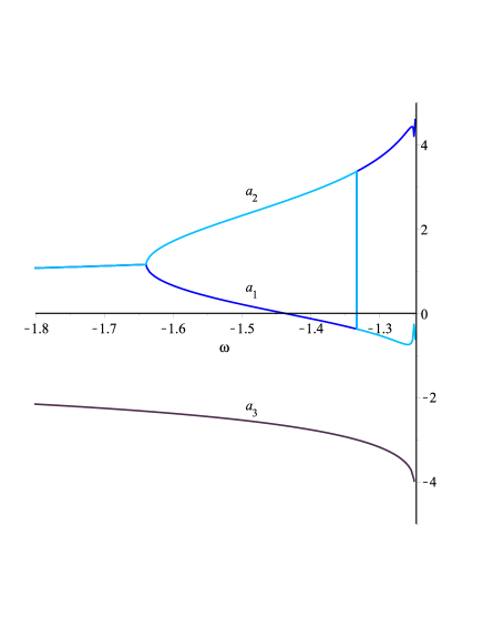
(a)

Figure 1: Real part of the eigenvalues corresponding to $P_{2+}$. The curves corresponding to $a_{1}$ and $a_{2}$ are superposed to the left of approx. $\omega=-1.64$, and show a discontinuity at $\omega=-4/3$.

The plots show that there are no values of $\omega$ such that the real part of the three eigenvalues is real and negative. Consequently, $P_{2+}$ cannot be a stable point, and the behaviour of the system close to $P_{2+}$ cannot approach the one currently displayed by the $\Lambda$CDM model.

3.1.2 $P_{2-}$

The eigenvalues in this case are given by the following expressions:

$${a}_{1}(\omega) = \frac{1}{2(3\omega+4)(\omega+2)^{2}}\left[\sqrt{6}(1216+7296\omega+16600\omega^{2}+17600\omega^{3}+8151\omega^{4}+686\omega^{5}\right.$$

$$\left.-384\omega^{6}+\sqrt{-15-12\omega}\>(-64-128\omega+648\omega^{2}+1904\omega^{3}+1689\omega^{4}+496\omega^{5}))^{1/2}\right.$$

$$\left.+9\omega^{2}+30\omega+24+(3\omega^{2}+10\omega+8)\sqrt{-15-12\omega}\>\right],$$

$${a}_{2}(\omega)=\frac{3+\sqrt{-15-12\omega}}{\omega+2}-{a}_{1}(\omega),$$ (21)

$${a}_{3}(\omega)=-\frac{3+\sqrt{-15-12\omega}}{\omega+2}.$$ (22)

Fig. 2 shows the plots of the real part of each eigenvalue associated to $P_{2-}$.

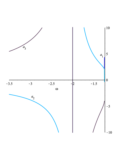
(a)

Figure 2: Real part of the eigenvalues corresponding to $P_{2-}$. The curves corresponding to $a_{1}$ and $a_{2}$ are not superposed only near $\omega=-1.25$, and show a divergence for $\omega=-2$.

The plots show that there is no interval of values of $\omega$ such that the real part of the three eigenvalues is negative.

3.2 ${\bf P_{5\pm}}$

The critical points $P_{5\pm}$ depend of the potential through the condition $\lambda=\beta$. Since the eigenvalues for arbitrary values of $\omega$ and $\beta$ are given by long algebraic expressions, we restrict here to the potential $V(\phi)=V_{0}\phi^{n}$, such that $\beta=\lambda=-n$ for every value of $V_{0}$ and $n$. This choice is justified by the fact that several effective quantum field theories can be related to his kind of self–interacting potential Fujii2003 . In particular, we shall examine the cases $n=2$ and $n=4$, frequently considered in cosmological scenarios (see for instance Sen2003 ; Boisseau2016 ; Carloni2008 ).

3.2.1 $P_{5+}$

The real part of the eigenvalues corresponding to the critical point $P_{5+}$ are plotted in Fig. 3 for $n=2$ and $n=4$. None of the cases is associated to a stable critical point with $\dot{H}=0$.

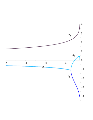
(a)

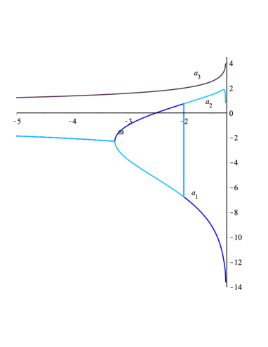
(b)

Figure 3: Real part of the eigenvalues corresponding to $P_{5+}$, for $n=2$ (left), and $n=4$ (right). The latter shows a discontinuity for $\omega=-2$. The plots for $a_{1}$ and $a_{2}$ are superposed for $\omega\lessapprox-1.7$ (left) and $\omega\lessapprox-3.2$ (right)

3.2.2 $P_{5-}$

The eigenvalues are plotted in Fig. 4 for $n=2$ and $n=4$, and they fail to comply with the condition that their real part be negative.

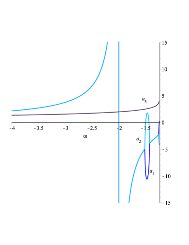
(a)

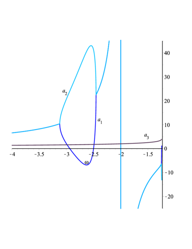
(b)

Figure 4: Real part of the eigenvalues corresponding to $P_{5-}$ and $n=2$ (left) and $n=4$ (right). $a_{1}$ and $a_{2}$ are singular at $\omega=-2$.

3.3 ${\bf P_{6}}$

The expression for the eigenvalues is in this case the following:

$$a_{1}(\omega)=-\frac{\left.\frac{d\Gamma(\lambda)}{d\lambda}\right|_{\lambda_{c}}+1}{\omega-1},$$ (23)

$$a_{2}(\omega)=a_{3}(\omega)=-\frac{4\omega+5}{\omega-1},$$ (24)

with $\Gamma(-1)=0$. The eigenvalues are shown in Fig. 5 for $\left.\frac{d\Gamma(\lambda)}{d\lambda}\right|_{\lambda_{c}}=-1.8$ . We see that, in spite of the fact that the real part of the three eigenvalues is negative, the eigenvalue $a_{1}$ could be associated to non-relativistic matter (i.e. is such that $Re(a_{1})=-3$) only for a unique value of $\omega$. Note that, although this conclusion follows from a particular value of $\left.\frac{d\Gamma(\lambda)}{d\lambda}\right|_{\lambda_{c}}$, the same will happen for any other value of the derivative compatible with the restrictions, due to the specific form of the dependence of $a_{1}$ with the derivative. Hence, $P_{6}$ should also be discarded.

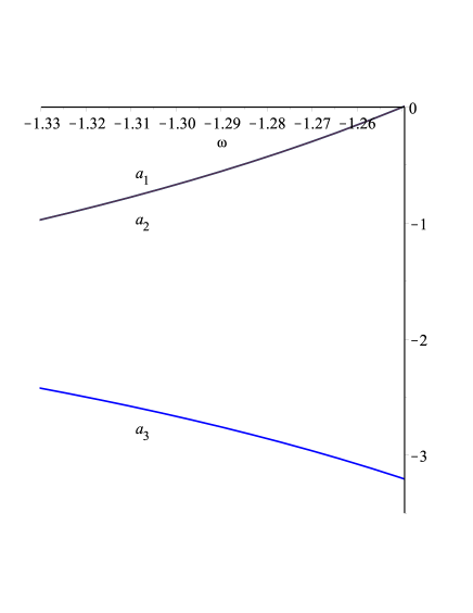
(a)

Figure 5: Plot of the real part of the eigenvalues corresponding to $P_{6}$, for $\left.\frac{d\Gamma(\lambda)}{d\lambda}\right|_{\lambda_{c}}=-1.8$ .

4 Discussion

We have examined whether a 4-dimensional universe in accelerated expansion and containing non-relativistic matter can be obtained by dimensional reduction of a self-interacting BD theory defined in $d=5$. The study required rewriting the equations of the system as an autonomous 3-dimensional dynamical system. The analysis of the eigenvalues of the linearized system shows that it has no stable equilibrium points subject to the condition $\dot{H}=0$, except for the critical point $P_{6}$, which is a stable critical point, but can describe non-relativistic matter only for a unique value of $\omega$ (given a value of $\left.\frac{d\Gamma(\lambda)}{d\lambda}\right|_{\lambda_{c}}$ compatible with the restrictions) . Hence, the model cannot mimic the $\Lambda$CDM dynamics. This conclusion was obtained in full generality for $P_{2\pm}$ and $P_{6}$, and for $V(\phi)=V_{0}\phi^{n}$ and $n=2,4$ in the case of $P_{5\pm}$. The failure of the model presented here in describing both the accelerated expansion and the matter content of the 4-dimensional universe should perhaps be taken as an indication that more complex models are needed, such as those in presented in PoncedeLeon2010 , where the metric coefficient of the extra dimension is a function of both time and the extra coordinate. We hope to go back to these ideas in a future publication.

References

- [1] Alves Joao, Combes Françoise, Ferrara Andrea, Forveille Thierry, and Shore Steve. Planck 2015 results. A&A, 594:E1, 2016.
- [2] Joshua Frieman, Michael Turner, and Dragan Huterer. Dark Energy and the Accelerating Universe. Ann. Rev. Astron. Astrophys., 46:385–432, 2008.
- [3] Sean M. Carroll. Why is the universe accelerating? eConf, C0307282:TTH09, 2003. [AIP Conf. Proc.743,16(2005)].
- [4] Li Miao, Li Xiao-Dong, Wang Shuang, and Wang Yi. Dark energy. Communications in Theoretical Physics, 56(3):525, 2011.
- [5] Timothy Clifton, Pedro G. Ferreira, Antonio Padilla, and Constantinos Skordis. Modified Gravity and Cosmology. Phys. Rept., 513:1–189, 2012.
- [6] Krzysztof Bolejko and Mikołaj Korzyński. Inhomogeneous cosmology and backreaction: current status and future prospects. 2016.
- [7] P. S. Wesson. Five-dimensional physics: Classical and quantum consequences of Kaluza-Klein cosmology. 2006.
- [8] Paul S. Wesson and J. Ponce de Leon. Kaluza–klein equations, einstein’s equations, and an effective energy-momentum tensor. Journal of Mathematical Physics, 33(11):3883–3887, 1992.
- [9] J. Ponce de Leon. Late time cosmic acceleration from vacuum Brans-Dicke theory in 5D. Class. Quant. Grav., 27:095002, 2010.
- [10] L. M. Reyes and J. E. Madriz Aguilar. Embedding General Relativity with varying cosmological constant term in five-dimensional Brans-Dicke theory of gravity in vacuum. ArXiv e-prints, February 2009.
- [11] J. Ponce de Leon. Brans-Dicke Cosmology in 4D from scalar-vacuum in 5D. JCAP, 1003:030, 2010.
- [12] Amir F. Bahrehbakhsh, Mehrdad Farhoudi, and Hossein Shojaie. FRW Cosmology From Five Dimensional Vacuum Brans-Dicke Theory. Gen. Rel. Grav., 43:847–869, 2011.
- [13] S. M. M. Rasouli, M. Farhoudi, and H. R. Sepangi. An anisotropic cosmological model in a modified Brans-Dicke theory. Classical and Quantum Gravity, 28(15):155004, August 2011.
- [14] S. M. M. Rasouli and Paulo Vargas Moniz. Exact Cosmological Solutions in Modified Brans-Dicke Theory. Class. Quant. Grav., 33(3):035006, 2016.
- [15] Li-e Qiang, Yong-ge Ma, Mu-xin Han, and Dan Yu. 5-dimensional Brans-Dicke theory and cosmic acceleration. Phys. Rev., D71:061501, 2005.
- [16] Amir F. Bahrehbakhsh, Mehrdad Farhoudi, and Hajar Vakili. Dark Energy From Fifth Dimensional Brans-Dicke Theory. Int. J. Mod. Phys., D22:1350070, 2013.
- [17] Ahmad Borzou, Hamid Reza Sepangi, Shahab Shahidi, and Razieh Yousefi. Brane f(R) gravity. Europhys. Lett., 88(2):29001, 2009.
- [18] Antonio Troisi. Higher-order gravity in higher dimensions: Geometrical origins of four-dimensional cosmology? Eur. Phys. J., C77(3):171, 2017.
- [19] Pedro H. R. S. Moraes. Cosmological solutions from Induced Matter Model applied to 5D gravity and the shrinking of the extra coordinate. Eur. Phys. J., C75(4):168, 2015.
- [20] C. Santos and R. Gregory. Cosmology in Brans-Dicke Theory with a Scalar Potential. Annals of Physics, 258:111–134, July 1997.
- [21] S. Sen and T. R. Seshadri. Self Interacting Brans-Dicke Cosmology and Quintessence. International Journal of Modern Physics D, 12:445–460, 2003.
- [22] W. Chakraborty and U. Debnath. Role of Brans-Dicke Theory with or without Self-Interacting Potential in Cosmic Acceleration. International Journal of Theoretical Physics, 48:232–247, January 2009.
- [23] L. Perivolaropoulos. Equation of state of the oscillating brans-dicke scalar and extra dimensions. Phys. Rev. D, 67:123516, Jun 2003.
- [24] S. M. M. Rasouli, Mehrdad Farhoudi, and Paulo Vargas Moniz. Modified Brans–Dicke theory in arbitrary dimensions. Classical and Quantum Gravity, 31:115002, 2014.
- [25] Orest Hrycyna and Marek Szydlowski. Brans-Dicke theory and the emergence of CDM model. Phys. Rev., D88(6):064018, 2013.
- [26] Orest Hrycyna and Marek Szydlowski. Uniting cosmological epochs through the twister solution in cosmology with non-minimal coupling. JCAP, 1012:016, 2010.
- [27] Y. Fujii and K.-I. Maeda. The Scalar-Tensor Theory of Gravitation. March 2003.
- [28] B. Boisseau, H. Giacomini, and D. Polarski. Bouncing universes in scalar-tensor gravity around conformal invariance. Journal of Cosmology and Astroparticle Physics, 5:048, May 2016.
- [29] S. Carloni, J. A. Leach, S. Capozziello, and P. K. S. Dunsby. Cosmological dynamics of scalar tensor gravity. Classical and Quantum Gravity, 25(3):035008, February 2008.