ProSLAM: Graph SLAM from a Programmer’s Perspective

Abstract

In this paper we present ProSLAM, a lightweight stereo visual SLAM system designed with simplicity in mind. Our work stems from the experience gathered by the authors while teaching SLAM to students and aims at providing a highly modular system that can be easily implemented and understood. Rather than focusing on the well known mathematical aspects of Stereo Visual SLAM, in this work we highlight the data structures and the algorithmic aspects that one needs to tackle during the design of such a system. We implemented ProSLAM using the C++ programming language in combination with a minimal set of well known used external libraries. In addition to an open source implementation, we provide several code snippets that address the core aspects of our approach directly in this paper. The results of a thorough validation performed on standard benchmark datasets show that our approach achieves accuracy comparable to state of the art methods, while requiring substantially less computational resources.

I Introduction

Simultaneous Localization and Mapping (SLAM) systems manage to deliver incredible results and after years of extensive investigation, this topic still captures the imagination of many young students and prospective researchers. Among others ORB-SLAM2 [1] and LSD-SLAM [2] are the two main approaches that are regarded as the state of the art in the robotic community. The increasing sophistication of these systems generally comes at a price of higher complexity. This fact renders those systems hard to understand and extend for people new to the field.

In this paper we present ProSLAM (Programmers SLAM), a complete stereo visual SLAM system that combines well known techniques, encapsulating them in separated components with clear interfaces. We further provide code snippets that can be copied and pasted to realize core functionalities of the system. ProSLAM is implemented in C++ and makes minimal use of the basic functionalities of well known libraries such as Eigen, for matrix calculation, OpenCV for input output operation and feature extraction, and g2o [3] for pose graph optimization.

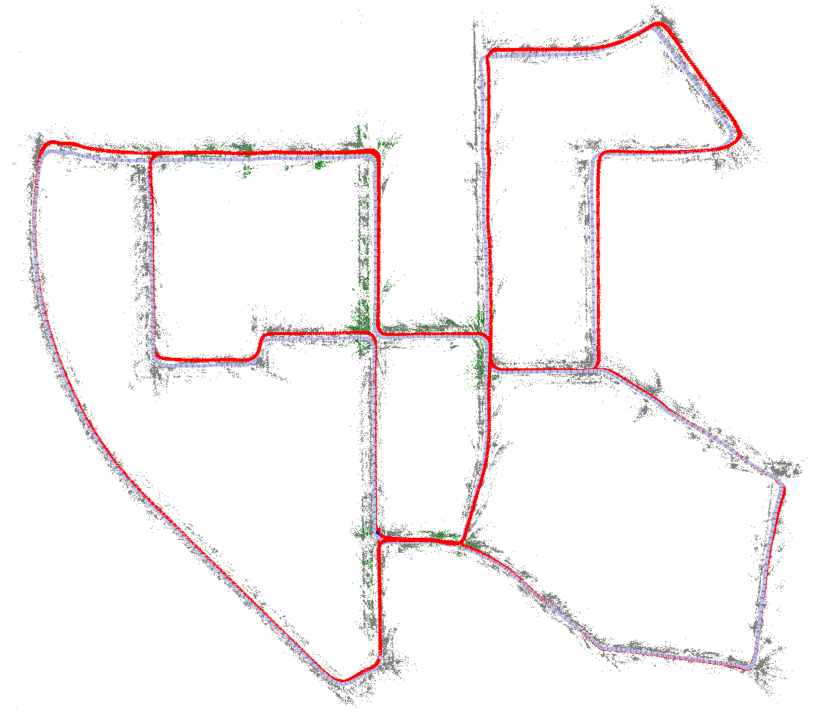
(a) KITTI Sequence 00, Blue trajectory: ours, Red: ground truth

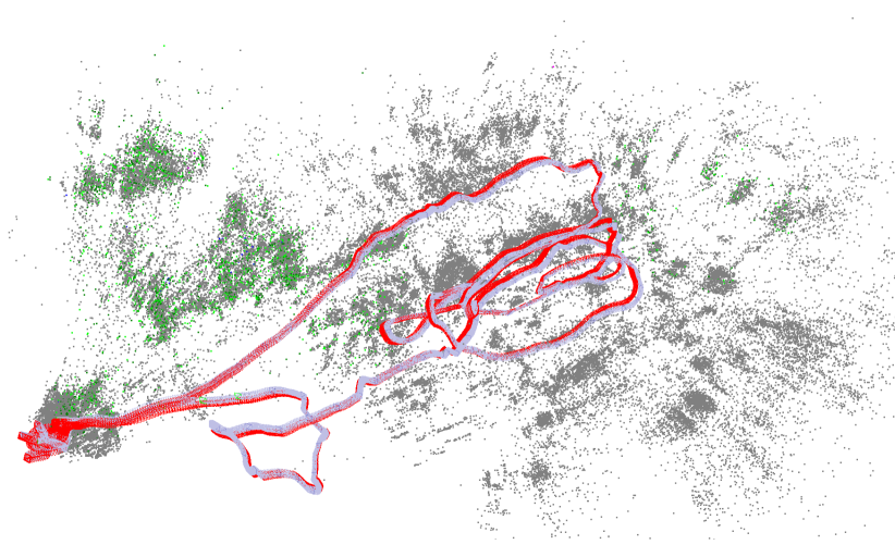
(b) EuRoC MH_01_easy, Blue trajectory: ours, Red: ground truth

Figure 1: Final map output of ProSLAM for two different datasets using identical parameters. The robot trajectory is illustrated by the light blue rectangular frame trail. Loop closed point clouds are highlighted in green.

We choose to operate on a stereo setting since the monocular case is substantially more complex as it requires to deal with proper initialization of the features and has to handle scale drift. Coping with these two aspects would add additional complexity that requires more advanced computer vision skills. Yet a stereo visual SLAM system is sufficiently usable to engage the students to continue learning in this field. Our system processes rectified and undistorted stereoscopic images, thus preventing the programmer from the need of handling the lens distortion and having to handle the stereo camera geometry. This comes at the cost of a slightly lower accuracy, but our experiments show that despite this simplification one can still achieve a high performance.

Similar to ORB-SLAM, our approach is feature based: it tracks a few features in the scene and thanks to the known geometry of the stereo cameras it determines the 3D position of the corresponding points. The image points tracked along multiple subsequent frames are grouped to form landmarks, that are salient points in the 3D spaces characterized by an appearance. The landmarks observed along a small portion of the trajectory are grouped in small point clouds (local maps) and the local maps themselves are arranged in a pose graph. This pose-graph [4] offers a deformable spatial backbone for the local maps that can be altered whenever the robot revisits a known location and identifies the current local map similar to an old one. Albeit the different modules of our system could be easily parallelized, we suggest a single threaded implementation, thus avoiding the complexity induced by synchronizing multiple threads and preserving the integrity of the memory.

Yet with this straightforward non parallel pipeline and with other further simplifications, such as the absence of any bundle adjustment stage in the system, our approach achieves accuracy comparable to the one of state of the art algorithms. Furthermore ProSLAM has substantially lower computational requirements. We performed comparative experiments on standard benchmarking datasets acquired from heterogeneous platforms, namely cars and quadrotors. Figure 1 shows the outcome of our approach while processing standard KITTI and EuRoC datasets acquired with different platforms Finally, we contribute to the community by providing an overseeable yet complete open-source SLAM system which can compete with the state of the art.

II Related Work

In the remainder of this section we discuss a selection of large-scale stereo visual SLAM systems and highlight their similarities and differences with respect to our approach. One of the first online large-scale stereo visual SLAM that appeared in literature is FrameSLAM. Konolige and Agrawal [5] introduced a complete feature based SLAM system with bundle adjustment running in real-time. For their approach they use CenSure features and integrate IMU information into the odometry computation. FrameSLAM proposed similar notions of system components like the ones of our system.

Pire et al. [6] presented a compact, appearance based stereo visual method S-PTAM. S-PTAM runs on 2 threads in real-time using the same BRIEF features as we do for tracking. Where g2o [3] is used for full bundle adjustment. In contrast to the other presented algorithms S-PTAM is not performing explicit relocalization and relies on full bundle adjustment for preserving the map consistency thus resulting in growing complexity as the size of the mapping environment increases.

Mur-Artal and Tardos [1] recently introduced an excellent, open source stereo visual SLAM system they named ORB-SLAM2. The system originated from the prominent, monocular ORB-SLAM published by the same authors. ORB-SLAM2 achieves extraordinary performance on standard datasets thanks to a highly reliable tracking front end and frequent relocalization using ORB features. Mur-Artal defines compact objects some of which directly correspond to objects in ProSLAM (e.g. landmarks). The system manages to close loops in real-time by utilizing a bag of words approach first proposed by Galvez-Lopez and Tardos [7]. ORB-SLAM2 employs g2o [3] for local bundle adjustment. The ORB-SLAM2 pipeline is designed to run on 3 parallel threads, increasing the complexity of the system layout.

Stereo LSD-SLAM proposed by Engel et al. [2] is a direct, featureless SLAM approach operating in large-scale at high processing speeds faster than real-time on a single thread. Engel exploits static and temporal stereo image changes at pixel level while also considering lightning changes.

In contrast to these approaches, that aim at advancing the state of the art at the cost of increasing complexity, ProSLAM is designed to be easy to understand and implement. Yet our system achieves comparable accuracy and has equal or lower computational requirements.

III Our Approach

The goal of ProSLAM is to process sequences of stereo image pairs to generate a 3D map. This map should represent the environment perceived by the robot and support crucial functionalities required in a SLAM system. The basic geometric entity that constitutes a map is a landmark. A landmark is a salient 3D point in the world characterized by its appearance in all images that display the landmark. The appearance is captured by a descriptor so that landmarks that appear similar will also have a similar descriptor.

Landmarks acquired in a nearby region form a local map, which can be seen as a point cloud where each point (landmark) has multiple descriptors. The local maps are arranged spatially in a pose graph. Each node of a pose graph thus encodes a 3D isometry (rotation and translation), representing the pose of the corresponding local map in the world. Edges between local maps represent spatial constraints correlating local maps close in space. These constraints are generated either by tracking the camera motion between temporally subsequent local maps or by aligning local maps acquired at distant times as a consequence of relocalization events.

The core functionalities of a SLAM map are:

• Relocalization

• Adjustment

Relocalization is achieved by comparing descriptors of local maps. Arranging the local maps in a pose graph allows us to utilize existing factor graph optimization engines for adjustment. Furthermore they enable us to limit the size of the adjustment problem, compared to a full bundle adjustment approach, substantially reducing computational cost. This comes at the price of a loss in accuracy, however our experiments show that the approach presented in this paper still reaches state of the art performance.

The process of generating these local maps can be split in 4 self-contained modules illustrated in Fig. 2. Their main tasks executed in sequence are:

• Triangulation (III-B) - The Triangulation module takes a stereo pair of images as input and produces 3D points plus corresponding feature descriptors for the left and right image respectively. The collection of this output is stored in a structure which we name frame.

• Incremental Motion Estimation (III-C) - In the Incremental Motion Estimation module we process a pair of subsequent frames to subsequently obtain the pose of the current frame.

• Map Management (III-D) - The Map Management module consumes frames with known camera motion and generates local maps extending the pose graph and refining landmark positions.

• Relocalization (III-E) - Relocalization is done by seeking if the current local map appears similar to some other local map generated in the past. Upon a successful search we derive the spatial relations between them and update our entire world map.

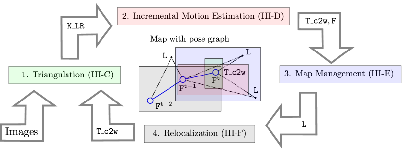
Figure 2: ProSLAM system overview with the 4 core modules. The only external input to the system are stereo images. Differently shaded areas of the central map show the components accessed by the respective modules.

In the following section we present an integrated overview over all major data structures of our system. We make use of C++ like pseudocode notation for introducing our data structures and code snippets to encourage direct re-usability.

III-A Data Structures

The sole inputs to our system are rectified, undistorted stereoscopic intensity images. Such Images are represented by a pair of 2D arrays containing intensity values and will be referred to as:

$$\mathtt{Image~{}I\_L},~{}\mathtt{I\_R}~{}\text{with}~{}\mathtt{I[r][c]}\in[0,1].$$

Where the subscripts $\mathtt{\_L}$ and $\mathtt{\_R}$ refer to the left respectively right camera of the stereo configuration. The integers $\mathtt{r/c}$ are equivalent to the pixel row/column indices of an image, also referred to as image coordinates.

We further introduce a more complex structure holding a feature’s keypoint and descriptor information:

⬇

KeypointWD {

int r; //image row of keypoint location

int c; //image column of keypoint location

float response; //keypoint response

Descriptor d; //corresponding descriptor

};

A KeypointWD (WD for WithDescriptor) $\mathtt{K}$ is created upon Feature Detection (III-B-1). The corresponding descriptor value $\mathtt{K.d}$ is set after Descriptor Extraction (III-B-3). The value $\mathtt{K.response}$ represents the ’goodness’ of a feature, a higher value indicating a more reliable redetection.

For these keypoints $\mathtt{K}$ we can retrieve epipolar correspondences to recover geometric information. The collection of data obtained during this process is stored in a so-called framepoint $\mathtt{P}$:

⬇

Framepoint {

KeypointWD k_L, k_R; //stereo keypoint+descriptor

Vector3 p_c; //3D coordinates in camera

Vector3 p_w; //3D coordinates in world

Framepoint *prev, *next; //track information

Landmark *landmark; //linked landmark

bool inlier; //pose opt. inlier status

};

By matching framepoints from the current image $\{\mathtt{P_{t}}\}$ against the ones from the previous image $\{\mathtt{P_{t-1}}\}$ we can determine which framepoints potentially originate from the same location in the real world. Once we found two such framepoints we link them by setting $\mathtt{P_{t}.prev}=\mathtt{P_{t-1}}$. These chains of framepoints are also called tracks and are derived inside the Incremental Motion Estimation module (III-C).

The Triangulation module usually manages to detect hundreds to thousands of good stereo point candidates in an Image pair, resulting in an approachingly high number of framepoints. The produced framepoints are accumulated in a frame $\mathtt{F}$:

⬇

Frame {

Image I_L, I_R; //raw image data

Transform T_c2w, T_w2c; //pose in world

Framepoint points[]; //present framepoints (owned)

Camera *cam_L, *cam_R; //cameras (stereo configuration)

};

In addition to the framepoints $\mathtt{F.points}$, a frame also holds the orientation and position estimate of the camera to the world $\mathtt{T\_c2w}$ for the given images $\mathtt{I\_L,R}$ at the time of its creation. The pose $\mathtt{T\_c2w}$ is also referred to as the frame pose and is always expressed respective to the world coordinate frame. Additionally a frame references a left and a right camera object, both capable of projecting framepoints Eq. (4) into an Image $\mathtt{I}$.

We further introduce the landmark structure $\mathtt{L}$:

⬇

Landmark {

Vector3 p_w; //landmark position in world

Framepoint *origin; //first sight of this landmark

Matrix3 omega; //information matrix

Vector3 nu; //information vector

};

Landmarks combine the information of a track of framepoints into a single entity. A landmark has one timeless position $\mathtt{L.p\_w}$, describing its currently estimated coordinates in the world frame. Using the $\mathtt{L.origin}$ field one has access to the first linked framepoint. The framepoint fields $\mathtt{P.next}$ and $\mathtt{P.prev}$ allow for easy navigation through the complete track history. In essence, landmarks can seen as framepoints with temporal information and are the closest property to a real world point. We favor landmarks over framepoints in two modules of our pipeline (III-C, III-E). Since landmarks exist over a sequence of images they are less affected by motion drift than framepoints and thus provide a more stable anchor for position estimation. The properties $\mathtt{omega}$ and $\mathtt{nu}$ are storing measurement information which is used in the information filter of the Landmark optimization phase.

For ProSLAM, we chose to bundle a set of subsequent frames together to perform reliable and fast relocalization (III-E). This bundling results in a local map object $\mathtt{M}$:

⬇

LocalMap {

Transform T_c2w, T_w2c; //pose of the local map in world

Frame frames[]; //enclosed frames (owned)

Landmark landmarks[]; //enclosed landmarks (shared)

};

A local map object $\mathtt{M}$ carries a transform information $\mathtt{M.T\_c2w}$, defined by the last frame in the collection of $\mathtt{M.frames}$. Additionally $\mathtt{M}$ holds a collection of direct references to the contained landmarks $\mathtt{L}$. Subsequently we define our global map object to be:

⬇

WorldMap {

Transform T_c2w, T_w2c; //world map origin

LocalMap maps[]; //enclosed local maps (owned)

Landmark landmarks[]; //enclosed landmarks (owned)

OptimizableGraph graph; //pose graph (g2o)

};

The world map defines the world coordinate frame for landmarks and local maps. The contained pose graph is used by the relocalization module to obtain optimized local map poses after adding a loop closure.

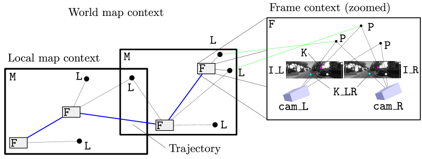
Figure 3: Schematic overview of our data structures. The trajectory is highlighted in blue, frames $\mathtt{F}$ and local maps $\mathtt{M}$ as rectangles and landmarks $\mathtt{L}$ as black dots. A stereo keypoint pair $\mathtt{K\_LR}$ (colored dots in images $\mathtt{I\_L}$, $\mathtt{I\_R}$) is visualized in the zoomed frame. The green lines connect framepoints $\mathtt{P}$ with their set landmark ($\mathtt{P.landmark}$).

III-B Triangulation

The goal of the Triangulation module is to process raw image data into a frame containing a cloud of framepoints. We assume the standard pinhole camera model [8] for all projection related operations. In a first stage we perform Feature Detection, returning keypoints $\mathtt{K\_L}$, $\mathtt{K\_R}$. To this extent we make use of the standard FAST keypoint detector [9]. In order to maintain a steady number of returned keypoints the FAST threshold is adjusted automatically at runtime (e.g. to obtain less points the value is raised and vice versa).

In a next phase we ensure that the keypoints are evenly distributed among the left image. The Regularization unit achieves this by first dividing all keypoints $\mathtt{K\_L}$ into bins arranged as a fine grid on the image. Subsequently only the keypoint with the highest $\mathtt{K.response}$ value in each bin is kept while discarding all the other keypoints. This operation heavily reduces the number of keypoints in the left image. On the right image we do not perform regularization in order to preserve the maximum number of potential candidates for the stereo point triangulation.

During the Descriptor Extraction the feature descriptors $\mathtt{K.d}$ are computed and set to $\mathtt{K\_L}$, $\mathtt{K\_R}$. For this purpose we use standard BRIEF descriptors [10], being a decent choice for real-time applications thanks to their robust and lightweight architecture.

Having $\mathtt{K\_L}$, $\mathtt{K\_R}$ with set descriptors allows us to perform an epipolar search for stereo keypoint pairs $\mathtt{K\_LR}$. This process is significantly simplified since we are working with undistorted and rectified images. In Lst. 1 we depict the implementation of the exact search procedure.

Listing 1: Stereo keypoint search

⬇

//Require: input arrays from left and right image

KeypointWD K_L[] = .., K_R[] = ..;

//Ensure: output array of stereo keypoint pairs

pair<KeypointWD, KeypointWD> K_LR[];

//sort all input vectors in the order of the expression

sort(K_L, ((K_L[i].r < K_L[j].r) ||

(K_L[i].r == K_L[j].r && K_L[i].c < K_L[j].c)));

sort(K_R, ((K_R[i].r < K_R[j].r) ||

(K_L[i].r == K_L[j].r && K_R[i].c < K_R[j].c)));

//configuration

const float maximum_matching_distance = ..;

int idx_R = 0;

//loop over all left keypoints

for (int idx_L = 0; idx_L < K_L.size(); idx_L++) {

//stop condition

if (idx_R == K_R.size()) {break;}

//the right keypoints are on an lower row - skip left

while (K_L[idx_L].r < K_R[idx_R].r) {

idx_L++; if (idx_L == K_L.size()) {break;}

}

//the right keypoints are on an upper row - skip right

while (K_L[idx_L].r > K_R[idx_R].r) {

idx_R++; if (idx_R == K_R.size()) {break;}

}

//search bookkeeping

int idx_RS = idx_R;

float dist_best = maximum_matching_distance;

int idx_best_R = 0;

//scan epipolar line for current keypoint at idx_L

while (K_L[idx_L].r == K_R[idx_RS].r) {

//zero disparity stop condition

if (K_R[idx_RS].c >= K_L[idx_L].c) {break;}

//compute descriptor distance

const float dist = hnorm(K_L[idx_L].d, K_R[idx_RS].d)

if(dist < dist_best) {

dist_best = dist;

idx_best_R = idx_RS;

}

idx_RS++;

}

//check if something was found

if (dist_best < maximum_matching_distance) {

K_LR += pair(K_L[idx_L], K_R[idx_best_R]);

idx_R = idx_best_R+1;

}

}

For an image point in the left frame ($\mathtt{r\_L,c\_L}$) the corresponding image point in the right frame ($\mathtt{r\_R,c\_R}$) must lie on a pixel column index ($\mathtt{c\_R}$) equal or less than the one from the left ($\mathtt{c\_L}$). This allows us to devise an efficient search strategy by ordering the keypoint vectors according to the lexicographical order of rows and columns (see Lst. 1). Once the vectors are sorted the search can be done in linear time. The $\mathtt{hnorm}$ function returns the Hamming distance between two descriptors. Upon completion, the Stereo keypoint search returns a set of stereo keypoint pairs $\mathtt{K\_LR}$.

Ultimately the keypoint pairs $\mathtt{K\_LR}$ are triangulated in order to obtain 3D points $\mathtt{p\_c}$. The computation of the depth $\mathtt{p\_c.z}$ based on a epipolar keypoint pair $(\mathtt{k\_L},\mathtt{k\_R})\in\mathtt{K\_LR}$ goes as follows:

$$\mathtt{p\_c.z}=\mathtt{B}/(\mathtt{k\_R.c}-\mathtt{k\_L.c})$$ (1)

Where $\mathtt{B}$ is the stereo camera baseline (pixels$\times$meters) and $\mathtt{k\_L.c}$ the left horizontal image coordinate of a keypoint pair $(\mathtt{k\_L},\mathtt{k\_R})$. Having the depth one can compute the $\mathtt{p\_c.x}$ and $\mathtt{p\_c.y}$ camera coordinates according to:

$$\mathtt{p\_c.x}=\mathtt{p\_c.z}/\mathtt{F\_x}*(\mathtt{k\_L.c}-\mathtt{C\_x})$$ (2)

$$\mathtt{p\_c.y}=\mathtt{p\_c.z}/\mathtt{F\_y}*(\mathtt{k\_L.r}-\mathtt{C\_y})$$ (3)

Where $\mathtt{F\_x,y}$ are the focal lengths and $\mathtt{C\_x}$, $\mathtt{C\_y}$ the principal points (pixels) of the left cameras projection matrix.

Once all keypoint pairs have been processed, the module packages each pair $(\mathtt{k\_L},\mathtt{k\_R})$ with its point $\mathtt{p\_c}$ into a framepoint $\mathtt{P}$. Fig. 4 shows the entire Triangulation module with inputs, outputs and its processing units.

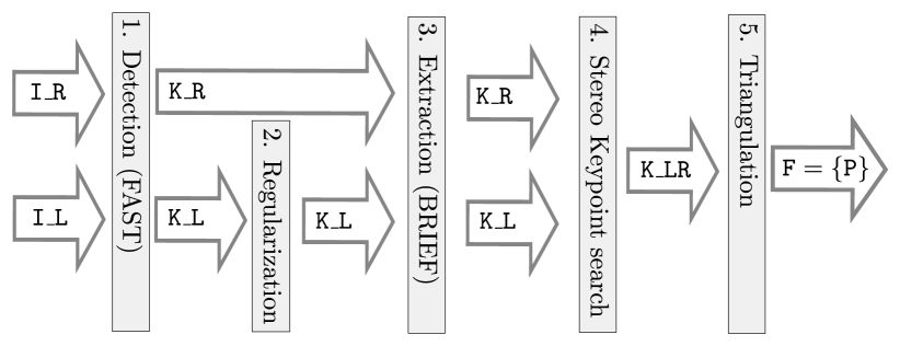
Figure 4: Triangulation (III-B) module. From left to to right, raw image data is transformed into an augmented 3D point cloud $\{\mathtt{P}\}$ contained in a frame object $\mathtt{F}$. Note that the keypoints from the right image are not filtered by the Regularization process.

III-C Incremental Motion Estimation

The goal of the Motion Estimation module is to determine the relative motion the left camera underwent, to get from a previous frame $\mathtt{F_{t-1}}$ to the current frame $\mathtt{F_{t}}$ in order to locate the current frame. That motion $\mathtt{T\_m}$ can be inferred as the same motion framepoints from the previous frame took, to appear in the current. Meaning that if we manage to connect framepoints in $\mathtt{F_{t}}$ with framepoints in $\mathtt{F_{t-1}}$ which stem from the same world point, we can compute the relative transform between them and subsequently find the pose $\mathtt{T\_c2w}$ of our current frame.

The task of finding these framepoint correspondences (tracks) is handled by the Tracking unit. We seek to find tracks based on projected image coordinates on the left camera only (monocular tracking). For this endeavor we first have to get the previous framepoints into the current image. A framepoint $\mathtt{P_{t-1}}$ from the previous frame is projected into the current left image $\mathtt{I\_L}$ as:

$$\mathtt{k\_P}=\pi(\mathtt{P\_L}*\mathtt{T\_w2c}*\mathtt{P_{t-1}.p\_w})$$ (4)

Where $\pi(\mathtt{p\_w})$ is the camera projection function [8] and $\mathtt{P\_L}$ the projection matrix of the left camera. The object $\mathtt{k\_P}$ can be interpret as a new keypoint, carrying the descriptor of the framepoint $\mathtt{P.k\_L.d}$. To obtain the initial pose estimate $\mathtt{T\_w2c}$ we use the constant velocity motion model:

$$\mathtt{T\_m} = \mathtt{F_{t-1}.T\_w2c}*\mathtt{F_{t-2}.{(T\_w2c)}^{-1}}$$ (5)

$$\mathtt{T\_w2c} = \mathtt{T\_m}*\mathtt{F_{t-1}.T\_w2c}$$

If the frame $\mathtt{F_{t-2}}$ is not available we assume no motion and the prior becomes: $\mathtt{T\_w2c}=\mathtt{F_{t-1}.T\_w2c}$. This simple motion prediction model is sufficiently robust for systems with smooth motion and decent frame rates.

For each predicted keypoint $\mathtt{k\_P}$ from the previous frame we search for the keypoint $\mathtt{k\_L}$ in the current image that is closest to $\mathtt{k\_P}$. We restrict the search to a rectangular region around $\mathtt{k\_P}$ and we consider only those keypoint whose descriptors $\mathtt{k\_L.d}$ appear similar enough to $\mathtt{k\_P.d}$. The search is completed once each projection $\mathtt{k\_P}$ is matched to a keypoint $\mathtt{k\_L}$ or terminated if there are no more keypoints $\{\mathtt{k\_L}\}$ available to match to.

Given this set of matches we are able to determine the current camera pose. The Pose optimization utilizes the pose prior $\mathtt{T\_w2c}$, used to determine the keypoint matches, as initial guess and computes a refined estimate by minimizing the resulting projection errors in the image plane. Our complete Pose optimization algorithm is presented in Lst. 2.

Listing 2: Pose optimization

⬇

//Require: current frame (carrying framepoints)

Frame* frame = ..;

//Require|Ensure: transform estimate camera to/from world

Transform T_c2w = .., T_w2c = ..;

//ds configuration

const bool ignore_outliers = ..;

const float kernel_maximum_error = ..;

const float close_depth = ..;

const float maximum_depth = ..;

const int number_of_iterations = ..;

for (int i = 0; i < number_of_iterations; i++) {

//initialize least squares components

Matrix6 H = 0, Vector6 b = 0, Matrix4 omega = I;

//loop over all framepoints

for (Framepoint* fp: frame->points()) {

if (!fp->prev()) {continue;}

CameraCoordinates p_c = T_w2c*fp->prev()->p_w;

//preferably use landmark position estimate

if (fp->landmark()) {

p_c = T_w2c*fp->landmark()->p_w;

//increase weight for landmarks

omega = ..;

}

//project point into left and right image

const Keypoint k_L = frame->cam_L->project(p_c);

const Keypoint k_R = frame->cam_R->project(p_c);

//ds compute current reprojection error

const Vector4 error(k_L.u-fp->k_L.u, k_L.v-fp->k_L.v,

k_R.u-fp->k_R.u, k_R.v-fp->k_R.v);

//compute squared error

const float error_squared = error.transpose()*error;

//robust kernel

if (error_squared > kernel_maximum_error) {

if (ignore_outliers) {continue;}

omega *= kernel_maximum_error/error_squared;

} else {

fp->inlier = true;

}

//compute stereouv jacobian see Eq. (11)

Matrix4_6 J = getJacobian(T_w2c, p_c, frame);

//adjust omega: if the point is considered close

if(p_c.z() < close_depth) {

omega *= (close_depth-p_c.z())/close_depth;

} else {

omega *= (maximum_depth-p_c.z())/maximum_depth;

//disable contribution to translational error

J.block<3,3>(0,0) = 0;

}

//update H and b

H += J.transpose()*omega*J;

b += J.transpose()*omega*error;

}

//compute (Identity-damped) solution

const Vector6 dx = solve((H+I)\(-b));

T_w2c = v2t(dx)*T_w2c;

T_c2w = T_w2c.inverse();

}

Note that the Pose optimization algorithm checks if framepoints are connected to landmarks and if so, uses the landmark position $\mathtt{L.p\_w}$ instead of the framepoint position $\mathtt{P.p\_w}$ to compute the reprojections $\mathtt{k\_L},\mathtt{k\_L}$. After each iteration the current pose estimate $\mathtt{T\_c2w}$ is updated. The function $\mathtt{v2t}$ transforms the pose matrix from the smooth manifold representation [11] back to an isometry. For completeness we provide the complete stereo image point Jacobian:

$$\mathtt{J\_L} = \left[\begin{array}[]{ccc}\mathtt{1/c\_L}&\mathtt{0}&-\mathtt{a\_{L}/c\_{L}^{2}}\\ \mathtt{0}&\mathtt{1/c\_{L}}&-\mathtt{b\_{L}/c\_{L}^{2}}\end{array}\right]$$ (8)

$$\mathtt{J\_R} = \left[\begin{array}[]{ccc}\mathtt{1/c\_R}&\mathtt{0}&-\mathtt{a\_{R}/c\_{R}^{2}}\\ \mathtt{0}&\mathtt{1/c\_{R}}&-\mathtt{b\_{R}/c\_{R}^{2}}\end{array}\right]$$ (11)

$$\mathtt{J\_T} = \left[\begin{array}[]{cc}\mathtt{I}&\mathtt{-2\mathtt{*}skew(p\_c)}\\ \mathtt{0}~{}\mathtt{0}~{}\mathtt{0}&\mathtt{0}~{}\mathtt{0}~{}\mathtt{0}\end{array}\right]$$ (14)

$$\mathtt{J} = \left[\begin{array}[]{c}\mathtt{J\_L}*\mathtt{P\_L}\\ \mathtt{J\_R}*\mathtt{P\_R}\end{array}\right]*\mathtt{J\_T}$$ (17)

The coefficients $\mathtt{a\_L,R}$, $\mathtt{b\_L,R}$ and $\mathtt{c\_L,R}$ are the coordinates of $\mathtt{p\_c}$ in the left respective right image before the homogenous division. $\mathtt{P\_L}$ and $\mathtt{P\_R}$ stand for the left and right camera projection matrix. In this particular case $\mathtt{I}$ stands for the $3\times 3$ identity matrix. Fig. 5 shows an overview of the whole Incremental Motion Estimation module. The final pose estimate $\mathtt{T\_c2w}$ and framepoints having field $\mathtt{P.inlier}$ set to $\mathtt{true}$ are passed to the next module.

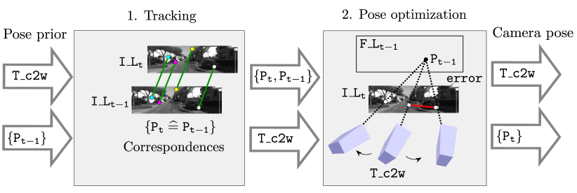
Figure 5: Incremental Motion Estimation (III-C) module. Overview of the incremental motion estimation for one timestep from previous Image $\mathtt{I\_L_{t-1}}$ to current Image $\mathtt{I\_L_{t}}$. The output framepoints $\{\mathtt{P_{t}}\}$ with corresponding previous framepoints $\{\mathtt{P_{t-1}}\}$ are connected by the $\mathtt{P.prev}$ field.

III-D Map Management

The Map Management module governs 3 main tasks in the following order:

1. Correspondence recovery

2. Landmark optimization

3. Local map generation

Correspondence recovery is an approach to locate previous framepoints in the current image by using the precise motion estimate resulting from the previous module (III-C). The set of candidates for Correspondence recovery is generated by bookkeeping of unmatched framepoints in the Tracking unit (III-C-1) of the Motion Estimation module. First we obtain the projection $\mathtt{k\_P}$ of the framepoint in the current image according to Eq. (4). Then the descriptor at $\mathtt{k\_P}$ is compared against $\mathtt{P.d\_L}$. If the matching distance is acceptable we confirm the correspondence and create a new framepoint linked to the previous one. Each time a landmark is observed, its estimate is refined by using a running information filter. A new local map is generated if one or both of the following properties exceed a certain threshold:

• Translation relative to previous local map

• Rotation relative to previous local map

For the generation of a local map the current frame pose $\mathtt{F.T\_c2w}$ is used also for the local map pose $\mathtt{M.T\_c2w}$. All other frames collected since the last Local map generation are scanned for landmarks and stored together in the new local map. The complete Map Management module can be inspected in Fig. 6.

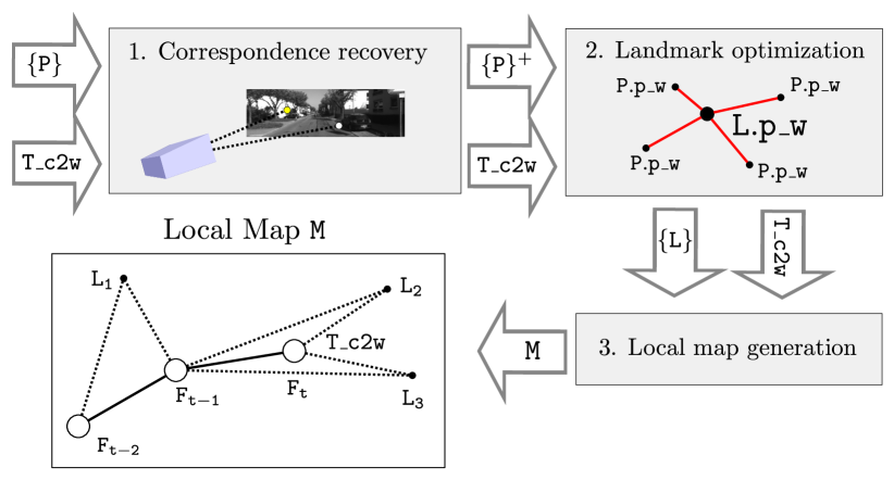
Figure 6: Map Management (III-D) module. Example sequence for the generation of a mocal map after 3 time steps (spanning over 3 frames).

III-E Relocalization

We want our system to recognize a previously traversed place and use this information to improve the position estimate of the current frame. A straightforward solution to this problem would be to compare each new frame against all past frames and attempt to retrieve a spatial constraint.

We chose to relocalize a current local map $\mathtt{M_{i}}$ only in past local maps $\mathtt{M_{j}}$, and not in single frames $\mathtt{F}$ to use the richness of the local map structure (e.g landmarks). Relocalization candidates are retrieved by comparing entire descriptor clouds from landmarks of local maps. With the goal of obtaining landmark to landmark correspondences. Searching correspondences with a similarity search is an expensive operation. Hence we do not directly look for correspondences but rather want to have a matching estimate of how much two local maps $\mathtt{M_{i}}$, $\mathtt{M_{j}}$ overlap first. And if this estimate is sufficiently high we perform the Similarity search. For both of these task we utilize the Hamming binary search tree library HBST [12].

The HBST library performs similarity search directly on descriptor to descriptor correspondences for two sets of descriptors. The search is performed efficiently by arranging the descriptor sets in a binary search tree, which is constructed after performing a probabilistic analysis on the descriptor bits. We use HBST’s descriptor to descriptor correspondences to retrieve landmark to landmark correspondences ($\mathtt{L_{M_{i}}}\mathrel{\widehat{=}}\mathtt{L_{M_{j}}}$). On $\mathtt{L_{M_{i}}}\mathrel{\widehat{=}}\mathtt{L_{M_{j}}}$ we run classic ICP [13] to achieve an Alignment. Giving us the relative transform $\mathtt{T\_i2j}$ between the local map poses $\mathtt{M_{i}}$, $\mathtt{M_{j}}$. The quality of the solution is defined by the final number of ICP inliers and the resulting average error. We discard transforms with a low inlier count and high average error in the Validation phase.

Validated relocalization constraints are introduced to the pose graph with a relaxed translational information value. The pose graph is optimized using g2o [3]. The optimized local map poses $\mathtt{M.T\_c2w}$ are broadcast to adjust the inner frame poses $\mathtt{F.T\_c2w}$. Landmark positions $\mathtt{L.p\_w}$ are moved rigidly according to their last relative location in the respective local map. Fig. 7 shows the entire Relocalization module and its interaction with the HBST library.

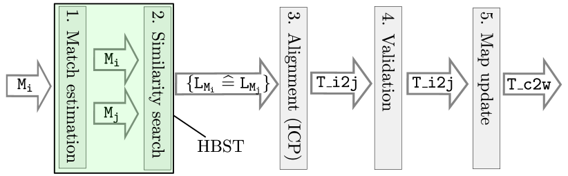
Figure 7: Relocalization (III-E) module. The sequence can be prematurely escaped at any unit, resulting in the loss of a global map update. In that case the transform $\mathtt{T\_c2w}$ does not change its value. If the module achieves a successful relocalization the global map as well as $\mathtt{T\_c2w}$ gets refined. The highlighted section area the use of HBST functionality.

IV Experimental Evaluation

The main focus of this work is to give the reader a clear insight into a complete, yet lightweight SLAM system while providing directly applicable code snippets accompanied by a solid performance confirmation.

All of our experiments are designed to show the capabilities of our system and to support our key proposals, such as having a functional, straightforward SLAM system running in a single thread. Which is capable of competing with state of the art algorithms in achieved precision while excelling at processing speed on ground vehicles and also works on airborne platforms.

We perform our evaluations on publicly available standard benchmark datasets. The KITTI SLAM evaluation presented by Geiger et al. [14] features challenging ground vehicle sequences in urban environments. We also tested ProSLAM on airborne vehicles in the recently published EuRoC MAV dataset collection of Burri et al. [15]. Our system runs with identical parameters throughout all of these experiments.

IV-A Trajectory Precision

The first experiment is designed to measure the precision of our approach. We report a quantitative as well as qualitative insights into the full KITTI evaluation, featuring 11 diverse mapping scenarios.

Figure 8: KITTI benchmark result comparison. Less is better.

From the translation error we can tell that our approach stands in the comparable range with the competing methods, outperforming LSD-SLAM in 7/11 and ORB-SLAM2 in 3/11 cases. Note that all tested methods achieve a relative error of less than 1% on average. As for the rotation error, we see that our system performs weaker than any of the compared methods, overcoming LSD-SLAM only in 2/11 and ORB-SLAM in 1/11 cases. We will address this issue in the Performance Analysis in Sec. IV-B.

Additionally we tested our approach on data recorded from an airborne vehicle. In Tab. I we report the accuracy of our system in the EuRoC MAV Dataset using only the stereo stream. We chose to display the absolute translation RMSE, being a clear indicator whether a SLAM system manages to produce an accurate trajectory or not.

TABLE I: EuRoC benchmark result comparison (RMSE)

Dataset	LSD-SLAM	ORB-SLAM2	ProSLAM
MH_01_easy	-	0.035	0.087
MH_02_easy	-	0.018	0.146
MH_03_medium	-	0.028	0.272
MH_04_difficult	-	0.119	-
MH_05_difficult	-	0.060	-
V1_01_easy	0.066	0.035	0.140
V1_02_medium	0.074	0.020	0.211
V1_03_difficult	0.089	0.048	-
V2_01_easy	-	0.037	-
V2_02_medium	-	0.035	-
V2_03_difficult	-	-	-

The values for LSD-SLAM and ORB-SLAM2 correspond to the values reported in the publications [2, 1]. For many challenging datasets our rudimentary motion model running on BRIEF features cannot adapt fast enough to the drones movement in the dark or blurred areas and the track breaks. The - sign indicates that the respective method was not able to finish the dataset.

IV-B Performance Analysis

The experimental evaluation confirms that our system provides competitive results in trajectory precision. ProSLAM shows a weakness in rotation estimation compared to state of the art approaches. This is a common odometry problem which is generally compensated by bundle adjustment. We tolerate this issue since our system does not feature bundle adjustment and the rotation error is still very low. On the other hand, we do not experience drift in pure translation due to the reliable depth values we obtain from the stereo camera setup. The overall system precision could have been further improved by the integration of error propagation models in loop closing, however to preserve clarity ProSLAM does not use any error kind of error modeling.

IV-C Processing Speed

The next experiment was chosen to support the claim that our approach can be executed fast enough to enable online processing on a single core CPU in real time. We ran all 11 KITTI benchmark sequences 10 times for each method, capturing start and end time. The benchmark computer setup consisted of a portable computer equipped with:

• Ubuntu 16.04 and OpenCV 3.1.1

• Intel i7-4700MQ CPU (4 cores, 3.4GHz, 6MB cache)

In the case of LSD-SLAM we report the values of the authors. Considering that Engel used a more powerful Intel i7-4900MQ CPU (4 cores, 3.8GHz, 8MB cache) for conducting the LSD-SLAM experiments [2].

TABLE II: KITTI: Average image processing speed

Approach	Threads	Mean duration (s)	Std. Dev (s)
LSD-SLAM	1	0.067	0.013
ORB-SLAM2	3	0.090	0.009
ProSLAM	1	0.059	0.010

By inspection of Tab. II one can see the speed advantage of ProSLAM. It is important to mention that LSD-SLAM and our system only use a single thread while ORB-SLAM2 occupies a total of 3 threads. All methods are able to process the KITTI datasets in real-time as the stereo camera images are provided at 10Hz.

V Conclusion

In this paper, we presented ProSLAM, a complete stereo visual SLAM system designed to be easily understood and implemented. We showed that a proper encapsulation of well known techniques in separated components with clear interfaces can lead to a very concise SLAM system. ProSLAM validates its efficient design by requiring only little computation resources while maintaining competitive precision and accuracy. We evaluated our approach on different datasets and provided comparisons to other existing techniques.

References

- [1] R. Mur-Artal and J. D. Tardos, “ORB-SLAM2: an Open-Source SLAM System for Monocular, Stereo and RGB-D Cameras,” arXiv preprint arXiv:1610.06475, 2016.
- [2] J. Engel, J. Stückler, and D. Cremers, “Large-scale direct SLAM with stereo cameras,” in Intelligent Robots and Systems (IROS), 2015 IEEE/RSJ International Conference on, pp. 1935–1942, IEEE, 2015.
- [3] R. Kümmerle, G. Grisetti, H. Strasdat, K. Konolige, and W. Burgard, “g2o: A general framework for graph optimization,” in Robotics and Automation (ICRA), 2011 IEEE International Conference on, pp. 3607–3613, IEEE, 2011.
- [4] G. Grisetti, R. Kümmerle, C. Stachniss, and W. Burgard, “A tutorial on graph-based SLAM,” Intelligent Transportation Systems Magazine, IEEE, vol. 2, no. 4, pp. 31–43, 2010.
- [5] K. Konolige and M. Agrawal, “FrameSLAM: From bundle adjustment to real-time visual mapping,” IEEE Transactions on Robotics, vol. 24, no. 5, pp. 1066–1077, 2008.
- [6] T. Pire, T. Fischer, J. Civera, P. De Cristóforis, and J. J. Berlles, “Stereo parallel tracking and mapping for robot localization,” in Intelligent Robots and Systems (IROS), 2015 IEEE/RSJ International Conference on, pp. 1373–1378, IEEE, 2015.
- [7] D. Gálvez-López and J. D. Tardos, “Bags of binary words for fast place recognition in image sequences,” IEEE Transactions on Robotics, vol. 28, no. 5, pp. 1188–1197, 2012.
- [8] R. Hartley and A. Zisserman, Multiple view geometry in computer vision. Cambridge university press, 2003.
- [9] E. Rosten and T. Drummond, “Machine learning for high-speed corner detection,” in European conference on computer vision, pp. 430–443, Springer, 2006.
- [10] M. Calonder, V. Lepetit, C. Strecha, and P. Fua, “Brief: Binary robust independent elementary features,” in European conference on computer vision, pp. 778–792, Springer, 2010.
- [11] R. C. Smith and P. Cheeseman, “On the representation and estimation of spatial uncertainty,” The international journal of Robotics Research, vol. 5, no. 4, pp. 56–68, 1986.
- [12] D. Schlegel and G. Grisetti, “Visual localization and loop closing using decision trees and binary features,” in Intelligent Robots and Systems (IROS), 2016 IEEE/RSJ International Conference on, pp. 4616–4623, IEEE, 2016.
- [13] P. J. Besl and N. D. McKay, “Method for registration of 3-D shapes,” in Robotics-DL tentative, pp. 586–606, International Society for Optics and Photonics, 1992.
- [14] A. Geiger, P. Lenz, and R. Urtasun, “Are we ready for autonomous driving? the kitti vision benchmark suite,” in Computer Vision and Pattern Recognition (CVPR), 2012 IEEE Conference on, pp. 3354–3361, IEEE, 2012.
- [15] M. Burri, J. Nikolic, P. Gohl, T. Schneider, J. Rehder, S. Omari, M. W. Achtelik, and R. Siegwart, “The EuRoC micro aerial vehicle datasets,” The International Journal of Robotics Research, vol. 35, no. 10, pp. 1157–1163, 2016.