Abstract

Weighted finite automata (WFA) can expressively model functions defined over strings but are inherently linear models. Given the recent successes of nonlinear models in machine learning, it is natural to wonder whether extending WFA to the nonlinear setting would be beneficial. In this paper, we propose a novel model of neural network based nonlinear WFA model (NL-WFA) along with a learning algorithm. Our learning algorithm is inspired by the spectral learning algorithm for WFA and relies on a nonlinear decomposition of the so-called Hankel matrix, by means of an auto-encoder network. The expressive power of NL-WFA and the proposed learning algorithm are assessed on both synthetic and real world data, showing that NL-WFA can lead to smaller model sizes and infer complex grammatical structures from data.

1 Introduction

Many tasks in natural language processing, computational biology or reinforcement learning, rely on estimating functions mapping sequences of observations to real numbers. Weighted finite automata (WFA) are finite state machines that allow one to succinctly represent such functions. WFA have been widely used in many fields such as grammatical parsing (Mohri and Pereira, 1998), sequence modeling and prediction (Cortes et al., 2004) and bioinfomatics (Allauzen et al., 2008). A probabilistic WFA (PFA) is a WFA satisfying some constraints that computes a probability distribution over strings; PFA are expressively equivalent to Hidden Markov Models (HMM) (Dupont et al., 2005), which have been successfully applied in many tasks such as speech recognition (Gales and Young, 2008) and human activity recognition (Nazábal and Artés-Rodríguez, 2015). Recently, the so-called spectral method has been proposed as an alternative to EM based algorithms to learn HMM (Hsu et al., 2009), WFA (Bailly et al., 2009), predictive state representations (Boots et al., 2011), and related models. Compared to EM based methods, the spectral method has the benefits of providing consistent estimators and reducing computational complexity.

Although WFA have been successfully applied in various areas of machine learning, they are inherently linear models: their computation boils down to the composition of linear maps. Recent positive results in machine learning have shown that models based on composing nonlinear functions are both very expressive and able to capture complex structure in data. For example, by leveraging the expressive power of deep convolutional neural networks in the context of reinforcement learning, agents can be trained to outperform humans in Atari games (Mnih et al., 2013) or to defeat world-class go players (Silver et al., 2016). Deep convolutional networks have also recently led to considerable breakthroughs in computer vision (Krizhevsky et al., 2012), where they showed their ability to disentangle the complex structure of the data by learning a representation which unfold the original complex feature space (where the data lies on a low-dimensional manifold) into a representation space where the structure has been linearized. It is thus natural to wonder to which extent introducing non-linearity in WFA could be beneficial. We will show that both these advantages of nonlinear models, namely their expressiveness and their ability to learn rich representations, can be brought to the classical WFA computational model.

In this paper, we propose a nonlinear WFA model (NL-WFA) based on neural networks, along with a learning algorithm. In contrast with WFA, the computation of a NL-WFA relies on successive compositions of nonlinear mappings. This model can be seen as an extension of dynamical recognizers (Moore, 1997) — which are in some sense a nonlinear extension of deterministic finite automata — to the quantitative setting. In contrast with the training of recurrent neural networks (RNN), our learning algorithm does not rely on back-propagation through time. It is inspired by the spectral learning algorithm for WFA, which can be seen as a two-step process: first find a low-rank factorization of the so called Hankel matrix leading to a natural embedding of the set of words into a low-dimensional vector space, and then perform regression in this representation space to recover the transition matrices. Similarly, our learning algorithm first finds a nonlinear factorization of the Hankel matrix using an auto-encoder network, thus learning a rich nonlinear representation of the set of strings, and then performs nonlinear regression using a feed-forward network to recover the transition operators in the representation space.

Related works. NL-WFA and RNN are closely related: their computation relies on the composition of nonlinear mappings directed by a sequence of observations. In this paper, we explore a somehow orthogonal direction to the recent RNN literature by trying to connect such models back with classical computational models from formal language theory. Such connections have been explored in the past in the non-quantitative setting with dynamical recognizers (Moore, 1997), whose inference has been studied in e.g. (Pollack, 1991). The ability of RNN to learn classes of formal languages has also been investigated, see e.g. (Avcu et al., 2017) and references therein. It is well know that predictive state representations (PSR) (Littman and Sutton, 2002) are strongly related with WFA (Thon and Jaeger, 2015). A nonlinear extension of PSR has been proposed for deterministic controlled dynamical systems in (Rudary and Singh, 2004). More recently, building upon reproducing kernel Hilbert space embedding of PSR (Boots et al., 2013), non-linearity is introduced into PSR using recurrent neural networks (Downey et al., 2017; Venkatraman et al., 2017). One of the main differences with these approaches is that our learning algorithm does not rely on back-propagation through time and we instead investigate how the spectral learning method for WFA can be beneficially extended to the nonlinear setting.

2 Preliminaries

We first introduce notions on weighted automata and the spectral learning method.

2.1 Weighted finite automaton

Let $\Sigma^{*}$ denote the set of strings over a finite alphabet $\Sigma$ and let $\lambda$ be the empty word. A weighted finite automaton (WFA) with $k$ states is a tuple $A=\langle\bm{\alpha}_{0},\bm{\alpha}_{\infty},\{\textbf{A}_{\sigma}\}\rangle$ where $\bm{\alpha}_{0},\bm{\alpha}_{\infty}\in\mathbb{R}^{k}$ are the initial and final weight vector respectively, and $\mathbf{A}_{\sigma}\in\mathbb{R}^{k\times k}$ is the transition matrix for each symbol $\sigma\in\Sigma$. A WFA computes a function $f_{A}:\Sigma^{*}\to\mathbb{R}$ defined for each word $x=x_{1}x_{2}\cdots x_{n}\in\Sigma^{*}$ by

$$f_{A}(x)=\bm{\alpha}_{0}^{\top}\mathbf{A}_{x_{1}}\mathbf{A}_{x_{2}}\cdots\mathbf{A}_{x_{n}}\bm{\alpha}_{\infty}.$$

By letting $\mathbf{A}_{x}=\mathbf{A}_{x_{1}}\mathbf{A}_{x_{2}}\cdots\mathbf{A}_{x_{n}}$ for any word $x=x_{1}x_{2}\cdots x_{n}\in\Sigma^{*}$ we will often use the shorter notation $f_{A}(x)=\mathbf{\bm{\alpha}}_{0}^{\top}\mathbf{A}_{x}\mathbf{\bm{\alpha}}_{\infty}.$ A WFA $A$ with $k$ states is minimal if its number of states is minimal, i.e., any WFA $B$ such that $f_{A}=f_{B}$ has at least $k$ states. A function $f:\Sigma^{*}\to\mathbb{R}$ is recognizable if it can be computed by a WFA. In this case the rank of $f$ is the number of states of a minimal WFA computing $f$. If $f$ is not recognizable we let $\operatorname*{rank}(f)=\infty$.

2.2 Hankel matrix

The Hankel matrix $\mathbf{H}_{f}\in\mathbb{R}^{\Sigma^{*}\times\Sigma^{*}}$ associated with a function $f:\Sigma^{*}\to\mathbb{R}$ is the bi-infinite matrix with entries $(\mathbf{H}_{f})_{u,v}=f(uv)$ for all words $u,v\in\Sigma^{*}$. The spectral learning algorithm for WFA relies on the following fundamental relation between the rank of $f$ and the rank of the Hankel matrix $\mathbf{H}_{f}$ (Carlyle and Paz, 1971; Fliess, 1974):

Theorem 1.

For any $f:\Sigma^{*}\to\mathbb{R}$, $\operatorname*{rank}(f)=\operatorname*{rank}(\mathbf{H}_{f})$.

In practice, one deals with finite sub-blocks of the Hankel matrix. Given a basis $\mathcal{B}=(\mathcal{P},\mathcal{S})\subset\Sigma^{*}\times\Sigma^{*}$, where $\mathcal{P}$ is a set of prefixes and $\mathcal{S}$ is a set of suffixes, we denote the corresponding sub-block of the Hankel matrix by $\mathbf{H}_{\mathcal{B}}\in\mathbb{R}^{\mathcal{P}\times\mathcal{S}}$. Among all possible basis, we are particularly interested in the ones with the same rank as $f$. We say that a basis is complete if $rank(\textbf{H}_{\mathcal{B}})=rank(f)=rank(\textbf{H}_{f})$.

For an arbitrary basis $\mathcal{B}=(\mathcal{P},\mathcal{S})$, we define its p-closure by $\mathcal{B}^{\prime}=(\mathcal{P^{\prime}},\mathcal{S})$, where $\mathcal{P^{\prime}}={\mathcal{P}}\cup\mathcal{P}\Sigma$. It turns out that a Hankel matrix over a p-closed basis can be partitioned into $|\Sigma|+1$ blocks of the same size (Balle et al., 2014):

$$\textbf{H}_{\mathcal{B}^{\prime}}^{\top}=[\textbf{H}_{\lambda}^{\top}|\textbf{H}_{\sigma_{1}}^{\top}|\cdots|\textbf{H}_{\sigma_{|\Sigma|}}^{\top}]$$

where for each $\sigma\in\Sigma\cup\{\lambda\}$ the matrix $\mathbf{H}_{\sigma}\in\mathbb{R}^{\mathcal{P}\times\mathcal{S}}$ is defined by $(\mathbf{H}_{\sigma})_{u,v}=f(u\sigma v)$.

2.3 Spectral learning

It is easy to see that the rank of the Hankel matrix $\mathbf{H}_{f}$ is upper bounded by the rank of $f$: if $A=\langle\bm{\alpha}_{0}^{\top},\bm{\alpha}_{\infty},\{\textbf{A}_{\sigma}\}\rangle$ is a WFA with $k$ states computing $f$, then $\mathbf{H}_{f}$ admits the rank $k$ factorization $\mathbf{H}_{f}=\mathbf{PS}$ where the matrices $\mathbf{P}\in\mathbb{R}^{\Sigma^{*}\times k}$ and $\mathbf{S}\in\mathbb{R}^{k\times\Sigma^{*}}$ are defined by $\mathbf{P}_{u,:}=\bm{\alpha}_{0}^{\top}\mathbf{A}_{u}$ and $\mathbf{S}_{:,v}=\mathbf{A}_{v}\bm{\alpha}_{\infty}$ for all $u,v\in\Sigma^{*}$. Moreover, one can check that $\mathbf{H}_{\sigma}=\mathbf{P}\mathbf{A}_{\sigma}\mathbf{S}$ for each $\sigma\in\Sigma$. The spectral learning algorithm relies on the non-trivial observation that this construction can be reversed: given any rank $k$ factorization $\mathbf{H}_{\lambda}=\mathbf{PS}$, the WFA $A=\langle\bm{\alpha}_{0}^{\top},\bm{\alpha}_{\infty},\{\textbf{A}_{\sigma}\}\rangle$ defined by

$$\bm{\alpha}_{0}^{\top}=\mathbf{P}_{\lambda,:},\ \ \bm{\alpha}_{\infty}=\mathbf{S}_{:,\lambda},\ \text{ and }\textbf{A}_{\sigma}=\textbf{P}^{+}\textbf{H}_{\sigma}\textbf{S}^{+},$$

is a minimal WFA computing $f$ (Balle et al., 2014, Lemma 4.1), where $\mathbf{H}_{\sigma}$ for $\sigma\in\Sigma\cup{\lambda}$ denote the finite matrices defined above for a prefix closed complete basis $\mathcal{B}$.

3 Nonlinear Weighted Finite Automata

The WFA model assumes that the transition operators $\mathbf{A}_{\sigma}$ are linear. It is natural to wonder whether this linear assumption sometimes induces a too strong model bias (e.g. if one tries to learn a function that is not recognizable by a WFA). Moreover, even for recognizable functions, introducing non-linearity could potentially reduce the number of states needed to represent the function. Consider the following example: given a WFA $A=\langle\bm{\alpha}_{0},\bm{\alpha}_{\infty},\{\textbf{A}_{\sigma}\}\rangle$, the function $(f_{A})^{2}:u\mapsto f_{A}(u)^{2}$ is recognizable and can be computed by the WFA $A^{\prime}=\langle\bm{\alpha}_{0}^{\prime},\bm{\alpha}_{\infty}^{\prime},\{\textbf{A}_{\sigma}^{\prime}\}\rangle$ with $\bm{\alpha}_{0}^{\prime}=\bm{\alpha}_{0}\otimes\bm{\alpha}_{0}$, $\bm{\alpha}_{\infty}^{\prime}=\bm{\alpha}_{\infty}\otimes\bm{\alpha}_{\infty}$ and $\textbf{A}_{\sigma}^{\prime}=\textbf{A}_{\sigma}\otimes\textbf{A}_{\sigma}$, where $\otimes$ denotes Kronecker product. One can check that if $\operatorname*{rank}(f_{A})=k$, then $\operatorname*{rank}(f_{A^{\prime}})$ can be as large as $k^{2}$, but intuitively the true dimension of the model is $k$ using non-linearity. These two observations motivate us to introduce nonlinear WFA (NL-WFA).

3.1 Definition of NL-WFA

We will use the notation $\tilde{g}$ to stress that a function $g$ may be nonlinear. We define a NL-WFA $\tilde{A}$ of with k states as a tuple $\langle\bm{\alpha}_{0},\tilde{G}_{\lambda},\{\tilde{{G}}_{\sigma}\}_{\sigma\in\Sigma}\rangle$, where $\bm{\alpha}_{0}\in\mathbb{R}^{k}$ is a vector of initial weights, $\tilde{{G}}_{\sigma}:\mathbb{R}^{k}\to\mathbb{R}^{k}$ is a transition function for each $\sigma\in\Sigma$ and $\tilde{G}_{\lambda}:\mathbb{R}^{k}\to\mathbb{R}$ is a termination function. A NL-WFA $\tilde{A}$ computes a function $f_{\tilde{A}}:\Sigma^{*}\to\mathbb{R}$ defined by

$$f_{\tilde{A}}(x)=\tilde{G}_{\lambda}(\tilde{G}_{x_{t}}(\cdots\tilde{G}_{x_{2}}(\tilde{G}_{x_{1}}(\mathbf{\bm{\alpha}}_{0}))\cdots))$$

for any word $x=x_{1}x_{2}\cdots x_{t}\in\Sigma^{*}$. Similarly to the linear case, we will sometimes use the shorthand notation $\tilde{G}_{x}=\tilde{G}_{x_{t}}\circ\tilde{G}_{x_{t-1}}\circ\cdots\circ\tilde{G}_{x_{1}}$. This nonlinear model can be seen as a generalization of dynamical recognizers (Moore, 1997) to the quantitative setting. It is easy to see that one recovers the classical WFA model by restricting the functions $\tilde{{G}}_{\sigma}$ and $\tilde{G}_{\lambda}$ to be linear. Of course some restrictions on these nonlinear functions have to be imposed in order to control the expressiveness of the model. In this paper, we consider nonlinear functions computed by neural networks.

3.2 A Representation learning perspective on the spectral algorithm

Our learning algorithm is inspired by the spectral learning method for WFA. In order to give some insights and further motivate our approach, we will first show how the spectral method can be interpreted as a representation learning scheme.

The spectral method can be summarized as a two-stages process consisting of a factorization step and a regression step: first find a low rank factorization of the Hankel matrix and then perform regression to estimate the transition operators $\{\mathbf{A}_{\sigma}\}_{\sigma\in\Sigma}$.

First focusing on the factorization step, let us observe that one can naturally embed the set of prefixes into the vector space $\mathbb{R}^{\mathcal{S}}$ by mapping each prefix $u$ to the corresponding row of the Hankel matrix $\mathbf{H}_{u,:}$. However, it is easy to check that this representation is highly redundant when the Hankel matrix is of low rank. In the factorization step of the spectral learning algorithm, the rank $k$ factorization $\mathbf{H}=\mathbf{PS}$ can be seen as finding a low dimensional representation $\mathbf{P}_{u,:}\in\mathbb{R}^{k}$ for each prefix $u$, from which the original Hankel representation $\mathbf{H}_{u,:}$ can be recovered using the linear map $\mathbf{S}$ (indeed $\mathbf{H}_{u,:}=\mathbf{P}_{u,:}\mathbf{S}$). We can formalize this encoder-decoder perspective by defining two maps $\Psi_{p}:\mathcal{P}\mapsto\mathbb{R}^{k}$ and $\Psi_{s}:\mathbb{R}^{k}\mapsto\mathbb{R}^{\mathcal{S}}$ by $\Psi_{p}(u)^{\top}=\mathbf{P}_{u,:}$ and $\Psi_{s}(\mathbf{x})^{\top}=\mathbf{x}^{\top}\mathbf{S}$. One can easily check that $\Psi_{s}(\Psi_{p}(u))^{\top}=\mathbf{H}_{u,:}$, which implies that $\Psi_{p}(u)$ encodes all the information sufficient to predict the value $f(uv)$ for any suffix $v\in\mathcal{S}$ (indeed $f(uv)=\Psi_{p}(u)^{\top}\mathbf{S}_{:,v}$).

The regression step of the spectral algorithms consists in recovering the matrices $\mathbf{A}_{\sigma}$ satisfying $\mathbf{H}_{\sigma}=\mathbf{P}\mathbf{A}_{\sigma}\mathbf{S}$. From our encoder-decoder perspective, this can be seen as recovering the compositional mappings $\mathbf{A}_{\sigma}$ satisfying $\Psi_{p}(u\sigma)^{\top}=\Psi_{p}(u)^{\top}\mathbf{A}_{\sigma}$ for each $\sigma\in\Sigma$.

It follows from the previous discussion that non-linearity could be beneficially brought to WFA and into the spectral learning algorithm in two ways: first by using nonlinear methods to perform the factorization of the Hankel matrix, thus discovering a potentially nonlinear embedding of the Hankel representation, and second by allowing the compositional feature maps associated to each symbol to be nonlinear.

4 Learning NL-WFA

Introducing non-linearity can be achieved in several ways. In this paper, we will use neural networks due to their ability to discover relevant nonlinear low-dimensional representation spaces and their expressive power as function approximators.

4.1 Nonlinear factorization

Introducing non-linearity in the factorization step boils down to finding two mappings $\Psi_{p}$ and $\Psi_{s}$ such that $\Psi_{s}(\Psi_{p}(u))=\mathbf{H}_{u,:}$ for any prefix $u\in\mathcal{P}$. Briefly going back to the linear case, one can check that if $\mathbf{H}=\mathbf{PS}$, then we have $\mathbf{H}_{u,:}=\mathbf{H}_{u,:}\mathbf{S}^{+}\mathbf{S}$ for each prefix $u$, implying that the encoder-decoder maps satisfy $\Psi_{p}(u)^{\top}=\mathbf{H}_{u,:}\mathbf{S}^{+}$ and $\Psi_{s}(\mathbf{x})^{\top}=\mathbf{x}^{\top}\mathbf{S}$. Thus the factorization step can essentially be interpreted as finding an auto-encoder able to project down the Hankel representation $\mathbf{H}_{u,:}$ to a low dimensional space while preserving the relevant information captured by $\mathbf{H}_{u,:}$.

How to extend the factorization step to the nonlinear setting should now appear clearly: by training an auto-encoder to learn a low-dimensional representation of the Hankel representations $\mathbf{H}_{u,:}$, one will potentially unravel a rich representation of the set of prefixes from which a NL-WFA can be recovered.

Let $\tilde{\phi}:\mathbb{R}^{\mathcal{S}}\mapsto\mathbb{R}^{k}$ and $\tilde{\phi}^{\prime}:\mathbb{R}^{k}\to\mathbb{R}^{\mathcal{S}}$ be the encoder and decoder maps respectively. We will train the auto-encoder shown in Figure 1 (left) to achieve

$$\tilde{\phi}^{\prime}(\tilde{\phi}(\mathbf{H}_{u,:}))\simeq\mathbf{H}_{u,:}.$$

More precisely, if $\textbf{H}\in\mathbb{R}^{m\times n}$, the model is trained to map the original Hankel representation $\mathbf{H}_{u,:}\in\mathbb{R}^{n}$ of each prefix $u$ to a latent representation vector in $\mathbb{R}^{k}$, where $k\ll n$, and then map this vector back to the original representation $\mathbf{H}_{u,:}$. This is achieved by minimizing the reconstruction error (i.e. the $\ell_{2}$ distance between the original representation and its reconstruction). Instead of linearly factorizing the Hankel matrix, we use an auto-encoder framework consisting of two networks, whose hidden layer activation functions are nonlinear.

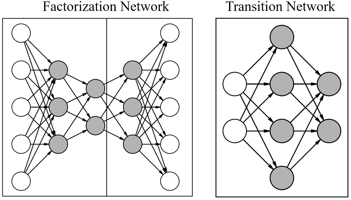
Figure 1: Factorization network and transition network: grey units are nonlinear while white ones are linear.

More precisely, if we denote the nonlinear activation function by $\theta$, and we let A, B, C, D be the weights matrices from the left to the right of the neural net shown in Figure 1 (left), the function $\hat{f}:\mathbb{R}^{n}\to\mathbb{R}^{n}$ computed by the auto-encoder can be written as

$$\hat{f}=\tilde{\phi^{\prime}}\circ\tilde{\phi}:\mathbf{(}\mathbf{H})_{u,:}^{\top}\mapsto\theta(\theta(\theta(\textbf{H}_{u,:}^{\top}\mathbf{A})^{\top}\textbf{B})^{\top}\mathbf{C})^{\top}\textbf{D}$$

where the encoder-decoder functions $\tilde{\phi}:\mathbb{R}^{n}\to\mathbb{R}^{k}$ and $\tilde{\phi^{\prime}}:\mathbb{R}^{k}\to\mathbb{R}^{n}$ are defined by $\tilde{\phi}(\mathbf{x})^{\top}=\theta(\theta(\mathbf{x}^{\top}\textbf{A})^{\top}\textbf{B})$ and $\tilde{\phi^{\prime}}(\mathbf{h})^{\top}=\theta({\mathbf{h}^{\top}}\textbf{C})^{\top}\textbf{D}$ for vectors $\mathbf{x}\in\mathbb{R}^{n},\mathbf{h}\in\mathbb{R}^{k}$.

It is easy to check that if the activation function $\theta$ is the identity, one will exactly recover a rank $k$ factorization of the Hankel matrix, thus falling back onto the classical factorization step of the spectral learning algorithm.

4.2 Nonlinear regression

Given the encoder-decoder maps $\tilde{\phi}$ and $\tilde{\phi^{\prime}}$, we then move on to recovering the transition functions. Recall that we wish to find the compositional feature maps $\tilde{G}_{\sigma}:\mathbb{R}^{k}\to\mathbb{R}^{k}$ for each $\sigma$ satisfying $\Psi_{p}(u\sigma)=\tilde{G}_{\sigma}(\Psi_{p}(u))$ for all $u\in{\mathcal{P}}$. Using the encoder map $\tilde{\phi}$ obtained in the factorization step, the mapping $\Psi_{p}$ can be written as $\Psi_{p}(u)=\tilde{\phi}(\mathbf{H}_{u,:})$.

In order to learn these transition maps, we will thus train one neural network for each symbol $\sigma$ to minimize the following squared error loss function

$$\sum_{u\in{\mathcal{P}}}\lVert\tilde{G}_{\sigma}(\tilde{\phi}(\mathbf{H}_{u,:}))-\tilde{\phi}(\mathbf{H}_{u\sigma,:})\rVert^{2}.$$

The structure of the simple feed-forward network used to learn the transition maps is shown in Figure 1 (right). Let $\mathbf{E},\mathbf{F}$ be the two weights matrices, the function $\hat{g}:\mathbb{R}^{k}\to\mathbb{R}^{k}$ computed by this network can be written as

$$\hat{g}:\mathbf{h}^{\top}\mapsto\theta(\theta(\mathbf{h}^{\top}\mathbf{E})^{\top}\mathbf{F})$$

We want to point out that both hidden units and output units of this network are nonlinear. Since this network will be trained to map between latent representations computed by the factorization network, the output units of the transition network and the units corresponding to the latent representation in the factorization network should be of the same nature to facilitate the optimization process.

4.3 Overall learning algorithm

Let $({\mathcal{P}},{\mathcal{S}})\subset\Sigma^{*}\times\Sigma^{*}$ be a basis of suffixes and prefixes such that $\lambda\in{\mathcal{P}}\cap{\mathcal{S}}$. Let $({\mathcal{P}}^{\prime},{\mathcal{S}})$ be its $p$-closure (i.e. ${\mathcal{P}}^{\prime}={\mathcal{P}}\cup{\mathcal{P}}\Sigma$) and let $m=|{\mathcal{P}}^{\prime}|,\ n=|{\mathcal{S}}|$. For reasons that will be clarified in the next section, we assume that ${\mathcal{P}}$ is prefix-closed (i.e. for any $x\in{\mathcal{P}}$, all prefixes of $x$ also belong to ${\mathcal{P}}$). The first step consists in building the estimate $\mathbf{H}\in\mathbb{R}^{m\times n}$ of the Hankel matrix from the training data (by using e.g. the empirical frequencies in the train set), where the rows of $\mathbf{H}$ are indexed by prefixes in ${\mathcal{P}}^{\prime}={\mathcal{P}}\cup{\mathcal{P}}\Sigma$ and its columns by suffixes in ${\mathcal{S}}$. The learning algorithm for NL-WFA then consists of two steps:

1. Train the factorization network to obtain a nonlinear decomposition of the Hankel matrix $\mathbf{H}$ through the mappings $\tilde{\phi}:\mathbb{R}^{n}\to\mathbb{R}^{k}$ and $\tilde{\phi}^{\prime}:\mathbb{R}^{k}\to\mathbb{R}^{n}$ satisfying

   $$\tilde{\phi}^{\prime}(\tilde{\phi}(\mathbf{H}_{u,:}))\simeq\mathbf{H}_{u,:}\ \ \text{for all }u\in{\mathcal{P}}\cup{\mathcal{P}}\Sigma.$$ (1)

2. Train the transition networks for each symbol $\sigma\in\Sigma$ to learn the transition maps $\tilde{G}_{\sigma}:\mathbb{R}^{k}\to\mathbb{R}^{k}$ satisfying

   $$\tilde{G}_{\sigma}(\tilde{\phi}(\mathbf{H}_{u,:}))\simeq\tilde{\phi}(\mathbf{H}_{u\sigma,:})\ \text{for all }u\in{\mathcal{P}}.$$ (2)

The resulting NL-WFA is then given by $\tilde{A}=\langle\mathbf{\bm{\alpha}}_{0},\tilde{G}_{\lambda},\{\tilde{G}_{\sigma}\}_{\sigma\in\Sigma}\rangle$ where $\bm{\alpha}_{0}=\tilde{\phi}(\mathbf{H}_{\lambda,:})$ and $\tilde{G}_{\lambda}$ is defined by

$$\tilde{G}_{\lambda}(\mathbf{x})=\bm{\lambda}^{\top}\tilde{\phi}^{\prime}(\mathbf{x})\ \text{for all }\mathbf{x}\in\mathbb{R}^{k}$$

where $\bm{\lambda}$ is the one-hot encoding of the empty suffix $\lambda$.

4.4 Theoretical analysis

While the definitions of the initial vector $\mathbf{\bm{\alpha}}_{0}$ and termination function $G_{\lambda}$ given above may seem ad-hoc, we will now show that the learning algorithm we derived corresponds to minimizing an error loss function between $f_{\tilde{A}}(u)$ and the estimated value $\mathbf{H}_{u,\lambda}$ over all prefixes in ${\mathcal{P}}$. Intuitively, this means that our learning algorithm aims at minimizing the empirical squared error loss over the training set ${\mathcal{P}}\subset\Sigma^{*}$. More formally, we show in the following theorem that if both the factorization network and the transition networks are trained to optimality (i.e. they both achieve $0$ training error), then the resulting NL-WFA exactly recovers the values given in the first column of the estimate of the Hankel matrix.

Theorem 2.

If the prefix set ${\mathcal{P}}$ is prefix-closed and if equality holds in Eq. (1) and Eq. (2), then the NL-WFA $\tilde{A}=\langle\mathbf{\bm{\alpha}}_{0},\tilde{G}_{\lambda},\{\tilde{G}_{\sigma}\}_{\sigma\in\Sigma}\rangle$, where $\bm{\alpha}_{0}=\tilde{\phi}(\mathbf{H}_{\lambda,:})$ and $\tilde{G}_{\lambda}:\mathbf{x}\mapsto\bm{\lambda}^{\top}\tilde{\phi}^{\prime}(\mathbf{x})$, is such that $f_{\tilde{A}}(u)=\mathbf{H}_{u,\lambda}$ for all $u\in{\mathcal{P}}$.

Proof.

We first show by induction on the length of a word $u=u_{1}u_{2}\cdots u_{t}\in{\mathcal{P}}$ that

$$\tilde{G}_{u}(\mathbf{\bm{\alpha}}_{0})=\tilde{G}_{u_{t}}(\tilde{G}_{u_{t-1}}(\cdots\tilde{G}_{1}(\mathbf{\bm{\alpha}}_{0})\cdots))=\tilde{\phi}(\mathbf{H}_{u,:}).$$

If $u=\sigma\in\Sigma$, using the fact that $\lambda\in{\mathcal{P}}$ we have $\tilde{G}_{\sigma}(\mathbf{\bm{\alpha}}_{0})=\tilde{G}_{\sigma}(\tilde{\phi}(\mathbf{H}_{\lambda,:}))=\tilde{\phi}(\mathbf{H}_{\sigma,:})$ by Eq. (2). Now if $u=u_{1}u_{2}\cdots u_{t}\in{\mathcal{P}}$, we can apply the induction hypothesis on $u_{1}u_{2}\cdots u_{t-1}$ (since ${\mathcal{P}}$ is prefix-closed) to obtain $\tilde{G}_{u}(\mathbf{\bm{\alpha}}_{0})=\tilde{G}_{u_{t}}(\tilde{G}_{u_{1}\cdots u_{t-1}}(\mathbf{\bm{\alpha}}_{0}))=\tilde{G}_{u_{t}}(\tilde{\phi}(\mathbf{H}_{u_{1}\cdots u_{t-1},:}))=\tilde{\phi}(\mathbf{H}_{u,:})$ by Eq. (2).

To conclude, for any $u\in{\mathcal{P}}$ we have $f_{\tilde{A}}(u)=\tilde{G}_{\lambda}(\tilde{G}_{u}(\mathbf{\bm{\alpha}}_{0}))=\tilde{G}_{\lambda}(\tilde{\phi}(\mathbf{H}_{u,:}))=\bm{\lambda}^{\top}\tilde{\phi}^{\prime}(\tilde{\phi}(\mathbf{H}_{u,:}))=\mathbf{H}_{u,:}\bm{\lambda}=\mathbf{H}_{u,\lambda}$ by Eq. (1).

∎

Intuitively, it follows that the learning algorithm described in Section 4.3 aims at minimizing the following loss function

$$J(\tilde{\phi},\tilde{\phi^{\prime}},\{\tilde{G}_{\sigma}\}_{\sigma\in\Sigma}) =\sum_{u\in{\mathcal{P}}}(\mathbf{\bm{\lambda}}^{\top}\tilde{\phi}^{\prime}(\tilde{G}_{u}(\tilde{\phi}(\mathbf{H}_{\lambda,:}))-\mathbf{H}_{u,\lambda})^{2}$$

$$=\sum_{u\in{\mathcal{P}}}(f_{\tilde{A}}(u)-\hat{f}(u))^{2}$$

where $\hat{f}(u)$ is the estimated value of the target function on the word $u$, and where the NL-WFA $\tilde{A}$ is a function of the encoder-decoder maps $\tilde{\phi},\tilde{\phi}^{\prime}$ and of the transition maps $\tilde{G}_{\sigma}$ as described in Section 4.3.

Even though Theorem 2 seems to suggest that our learning algorithm is prone to over-fitting, this is not the case. Indeed, akin to the linear spectral learning algorithm, the restriction on the number of states of the NL-WFA (which corresponds to the size of the latent representation layer in the factorization network) induces regularization and enforces the learning process to discriminate between signal and noise (i.e. in practice, the networks will not achieve $0$ error due to the bottleneck structure of the factorization network).

4.5 Applying non-linearity independently in the factorization and transition networks

We have shown that non-linearity can be introduced into the two steps of our learning algorithm. We can thus consider three variants of this algorithm where we either apply non-linearity in the factorization step only, in the regression step only, or in both steps. It is easy to check that these three different settings correspond to three different NL-WFA models depending on whether the termination function only is nonlinear, the transition functions only are nonlinear, or both the termination and transition functions are nonlinear. Indeed, recall that that a NL-WFA $\tilde{A}$ is defined as a tuple $\tilde{A}=\langle\bm{\alpha}_{0},\tilde{G}_{\lambda},\{\tilde{{G}}_{\sigma}\}_{\sigma\in\Sigma}\rangle$. If no non-linearity are introduced in the factorization network, the termination function will have the form

$$\tilde{G}_{\lambda}:\mathbf{x}\mapsto\mathbf{\bm{\lambda}}^{\top}\tilde{\phi}^{\prime}(\mathbf{x})=\mathbf{\bm{\lambda}}^{\top}\mathbf{D}^{\top}\mathbf{C}^{\top}\mathbf{x}$$

(using the notations from the previous sections), which is linear. Similarly, if no non-linearity are used in the transition networks, the resulting maps $\tilde{G}_{\sigma}$ will be linear.

One may argue that only applying non-linearity in the termination function $\tilde{G}_{\lambda}$ would not lead to an expressive enough model. However, it is worth noting that in this case, after the nonlinear factorization step, even though the transition functions are linear they are operating on a nonlinear feature space. This is similar in spirit to the kernel trick, where a linear model is learned in a feature space resulting from a nonlinear transformation of the initial input space. Moreover, if we go back to the example of the squared function $(f_{A})^{2}$ for some WFA $A$ with $k$ states (see beginning of Section 3), even though $(f_{A})^{2}$ may have rank up to $k^{2}$, one can easily build a NL-WFA with $k$ states computing $(f_{A})^{2}$ where only the termination function is nonlinear.

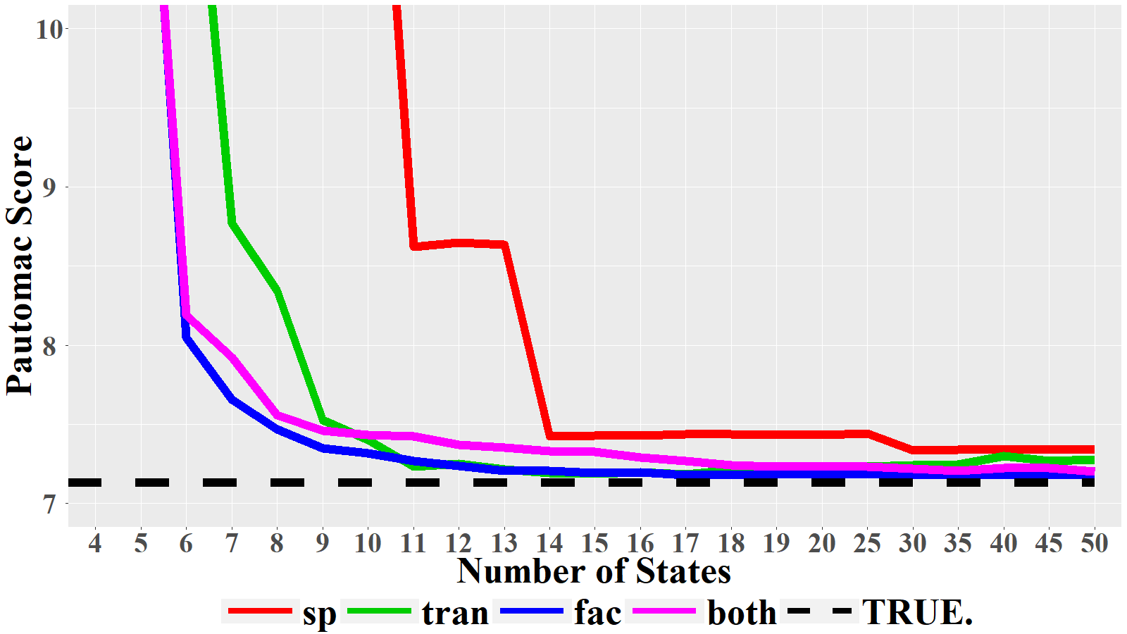
Figure 2: Pautomac score for the Dyck language experiment for different model sizes (trained on a sample size of 20,000).

5 Experiments

We compare the classical spectral learning algorithm with the three configurations of our neural-net based NL-WFA learning algorithms: applying non-linearity only in the factorization step (denoted by fac.non), only in the regression step (denoted by tran.non), and in both phases (denoted by both.non). We will perform experiments on a grammatical inference task (i.e. learn a distribution over $\Sigma^{*}$ from samples drawn from this distribution) with both synthetic and real data

5.1 Metrics

We use two metrics to evaluate the trained models on a test set: Pautomac score and word error rate.

• The Pautomac score was first proposed for the Pautomac challenge (Verwer et al., 2014) and is defined by

  $$\textit{Pauto}(M)=-2^{\sum_{x\in T}P_{\ast}(x)\log(P_{M}(x))}$$

  where $P_{M}(x)$ is the normalized probability assigned to $x$ by the learned model and $P_{\ast}(x)$ is the normalized true probability (both $P_{M}$ and $P_{\ast}$ are normalized to sum to $1$ over the test set $T$). Since the models returned by both our method and the spectral learning algorithm are not ensured to outputs positive values, while the logarithm of a negative value is not defined, we take the absolute values of all the negative outputs.

• The word error rate (WER) measures the percentage of incorrectly predicted symbols when, given each prefix of strings in the test set, the most likely next symbol is predicted.

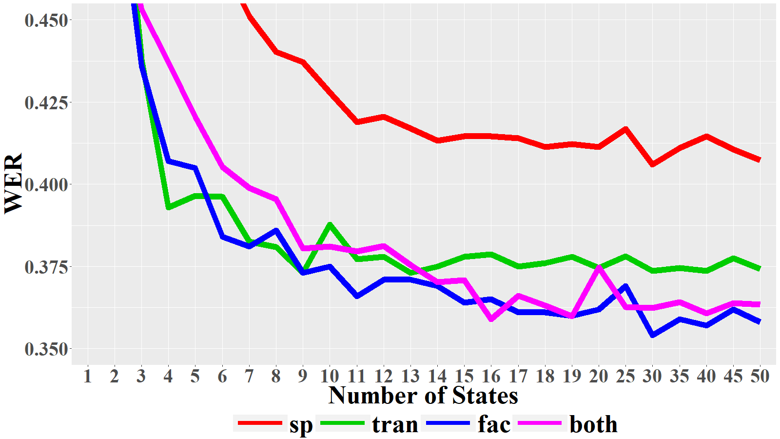
Figure 3: Word error rate for the Dyck language experiment for different model sizes (trained on a sample size of 20,000).

5.2 Synthetic data: probabilistic Dyck language

For the synthetic data experiment, we generate data from a probabilistic Dyck language. Let $\Sigma=\{[,]\}$, we consider the language generated by the following probabilistic context free grammar

$$S \to SS \text{ with probability }0.2$$

$$S \to[S] \text{ with probability }0.4$$

$$S \to[\ ] \text{ with probability }0.4$$

i.e. starting from the symbol $S$, we draw one of the rules according to their probability and apply it to transform $S$ into the corresponding right hand side; this process is repeated until no $S$ symbol are left. One can check that this distribution will generate balanced strings of brackets. It is well known that this distribution cannot be computed by a WFA (since its support is a context free grammar). However, as a WFA can compute any distribution with finite support, it can model the restriction of this distribution to word of length less than some threshold $N$. By using this distribution for our synthetic experiments, we want to showcase the fact that NL-WFA can lead to models with better predictive accuracy when the number of states is limited and that they can better capture the complex structure of this distribution.

In our experiments, we use empirical frequencies in a training data set to estimate the Hankel matrix $\mathbf{H}_{\mathcal{B}}\in\mathbb{R}^{1000\times 1000}$, where the p-closed basis $\mathcal{B}$ is obtained by selecting the $1,000$ most frequent prefixes and suffixes in the training data. We first assess the ability of NL-WFA to better capture the structure in the data when the number of states is limited. We compared the models for different model sizes $k$ ranging from $1$ to $50$, where $k$ is the number of states of the learned WFA and NL-WFA. For the latter, we used a three hidden layers structure for the factorization network where the number of hidden units are set to $2k$, $k$ and $2k$. For the transition networks, we use a neural network with $2k$ hidden units. We used Adamax (Kingma and Ba, 2014) with learning rate 0.015 and 0.001 respectively to train these two networks.

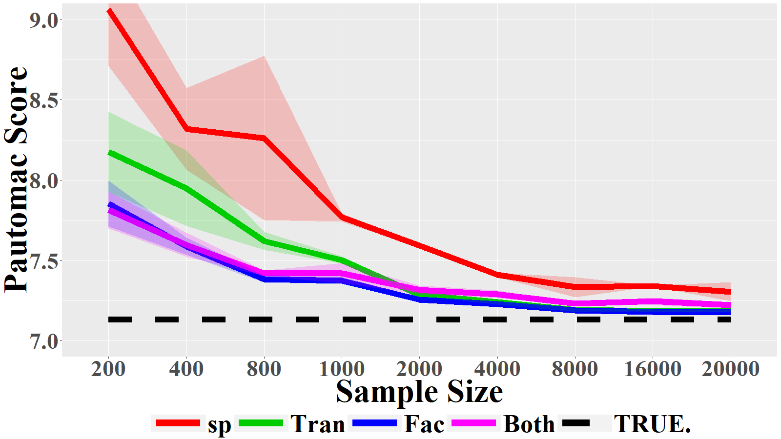
Figure 4: Average Pautomac score for learning the Dyck language with different sample sizes.

All models are trained on a training set of size $20,000$ and the Pautomac score and WER on a test set of size $250$ are reported in Figure 2 and 3 respectively. For both metrics, we see that NL-WFA gives better results for small model sizes. While NL-WFA and WFA tend to perform similarly for the Pautomac score for larger model sizes, NL-WFA clearly outperforms WFA in terms of WER in this case. This shows that including non-linearity can increase the prediction power of WFA by discovering the underlying nonlinear structure and can be beneficial when dealing with a small number of states.

We then compared the sample complexity of learning NL-WFA and WFA by training the different models on training set of sizes ranging from $200$ to $20,000$. For all models the rank is chosen by cross-validation. In Figure 4 and Figure 5, we show the performances for the four models on a test set of size $250$ by reporting the average and standard deviation over $10$ runs of this experiment. We can see that NL-WFA achieve better results on small sample sizes for the Pautomac score and consistently outperforms the linear model for all sample sizes for WER. This shows that NL-WFA can use the training data more efficiently and again that the expressiveness of NL-WFA is beneficial to this learning task.

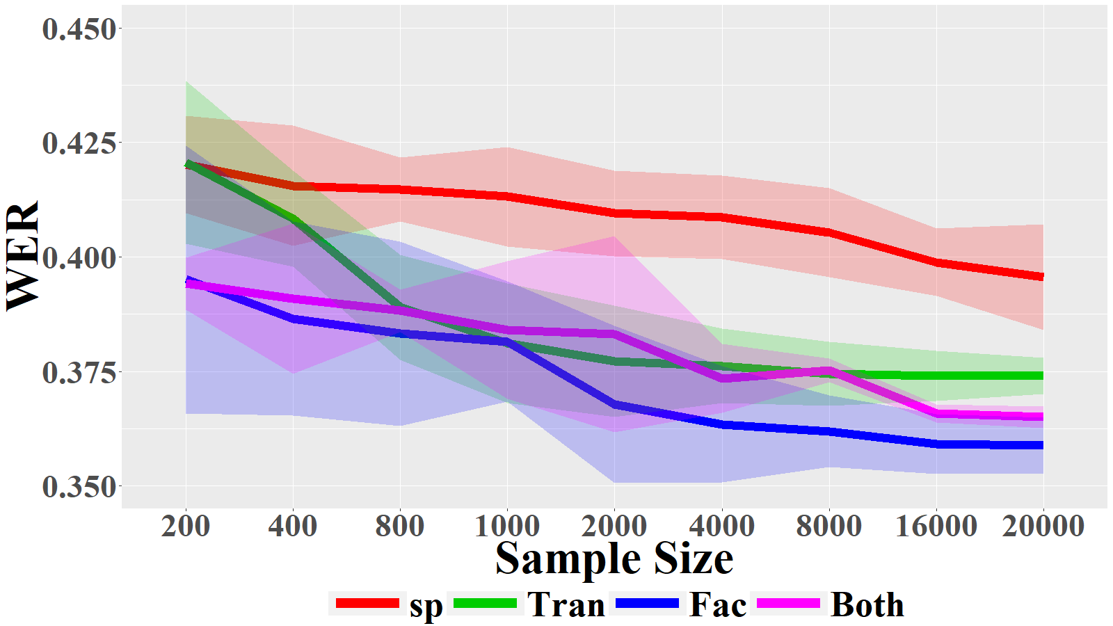
Figure 5: Average word error rate for learning the Dyck language with different sample sizes.

5.3 Real data: Penn treebank

The Penn Treebank (Taylor et al., 2003) is a well known benchmark dataset for natural language processing. It consists of approximately 7 million words of part-of-speech tagged text, 3 million words of skeletally parsed text, over 2 million words of text parsed for predicate argument structure, and 1.6 million words of transcribed spoken text annotated for speech disfluencies. In this experiment, we use a small portion of the Treebank dataset: the character level of English verbs which was used in the SPICE challenge (Balle et al., 2017). This dataset contains 5,987 sentences over an alphabet of 33 symbols as the training set. It also provides two test sets of size 750. We used one of the test sets as a validation set and then tested our models on the other.

For this experiment, the Hankel matrix $\mathbf{H}_{\cal B}$ is of size $3000\times 300$ where the prefixes and suffixes have been selected again by taking the most frequents in the training data. We used a five layers factorization network where the layers are of size $4k$, $2k$, $k$, $2k$ and $4k$ respectively, where $k$ is the number of states of the NL-WFA. The structure of the transition networks is the same as in the previous experiment. For all models, the rank is selected using the validation set.

In Table 1, we report the results for the two metrics on the test set. We can see that for both metrics, one of the NL-WFA models outperforms linear spectral learning. Individually speaking, for modeling the distribution (i.e. the perplexity metric) tran.non gives the best performances, while for the prediction task fac.non shows a significant advantage.

	SP	Tran.non	Fac.non	Both.non
log(Pauto)	21.3807	12.2571	13.8311	13.6604
WER	0.8033	0.8841	0.7061	0.8334

Table 1: Log perplexity and WER for real data

6 Discussion

We believe that trying to combine models from formal languages theory (such as weighted automata) and models that have recently led to several successes in machine learning (e.g. neural networks) is an exciting and promising line of research, both from the theoretical and practical sides. This work is a first step in this direction: we proposed a novel nonlinear weighted automata model along with a learning algorithm inspired by the spectral learning method for classical WFA. We showed that non-linearity can be introduced in two ways in WFA, in the termination function or in the transition maps, which directly translates into the two steps of our learning algorithm.

In our experiment, we showed on both synthetic and real data that (i) NL-WFA can lead to models with better predictive accuracy than WFA when the number of states is limited, (ii) NL-WFA are able to capture the complex underlying structure of challenging languages (such as the Dyck language used in our experiments) and (iii) NL-WFA exhibit better sample complexity when learning on data with a complex grammatical structure.

In the future, we intend to investigate further the properties of NL-WFA from both the theoretical and experimental perspectives. For the former, one natural question is whether we could obtain learning guarantees for some specific classes of nonlinear functions. Indeed, one of the main advantages of the spectral learning algorithm is that it provides consistent estimators. While it may be difficult to obtain such guarantees when considering functions computed by neural networks, we believe that studying the case of more tractable nonlinear functions (e.g. polynomials) could be very insightful. We also plan on thoroughly investigating connections between NL-WFA and RNN. From the practical perspective, we want to first tune the hyper-parameters for NL-WFA more extensively on the current datasets to potentially improve the results. In addition, we intend to run further experiments on real data and on different kinds of tasks beside language modeling (e.g. classification, regression). Moreover, due to the strong connection between WFA and PSR, it will be very interesting to use NL-WFA in the context of reinforcement learning.

It is worth mentioning that the spectral learning algorithm cannot straightforwardly be used to learn functions that are not probability distributions. Indeed, while it makes sense in the probabilistic setting to fill the entries corresponding to words that are not in the training data to $0$ in the Hankel matrix, it is not clear how to fill these entries when one wants to learn a function that is not a probability distribution, e.g. in a regression task. One way to circumvent this issue is to first use matrix completion techniques to fill these missing entries before performing the low rank decomposition of the Hankel matrix (Balle and Mohri, 2012). In contrast, our learning algorithm can directly be applied to this setting by simply adapting the loss function of the factorization network (i.e. simply ignore the missing entries in the loss function).

References

- Allauzen et al. [2008] Cyril Allauzen, Mehryar Mohri, and Ameet Talwalkar. Sequence kernels for predicting protein essentiality. In Proceedings of the 25th International Conference on Machine learning, pages 9–16. ACM, 2008.
- Avcu et al. [2017] Enes Avcu, Chihiro Shibata, and Jeffrey Heinz. Subregular complexity and deep learning. arXiv preprint arXiv:1705.05940, 2017.
- Bailly et al. [2009] Raphaël Bailly, François Denis, and Liva Ralaivola. Grammatical inference as a principal component analysis problem. In Proceedings of the 26th Annual International Conference on Machine Learning, pages 33–40. ACM, 2009.
- Balle and Mohri [2012] Borja Balle and Mehryar Mohri. Spectral learning of general weighted automata via constrained matrix completion. In Advances in Neural Information Processing Systems, pages 2159–2167, 2012.
- Balle et al. [2014] Borja Balle, Xavier Carreras, Franco M Luque, and Ariadna Quattoni. Spectral learning of weighted automata. Machine learning, 96(1-2):33–63, 2014.
- Balle et al. [2017] Borja Balle, Rémi Eyraud, Franco M Luque, Ariadna Quattoni, and Sicco Verwer. Results of the sequence prediction challenge (spice): a competition on learning the next symbol in a sequence. In International Conference on Grammatical Inference, pages 132–136, 2017.
- Boots et al. [2011] Byron Boots, Sajid M Siddiqi, and Geoffrey J Gordon. Closing the learning-planning loop with predictive state representations. The International Journal of Robotics Research, 30(7):954–966, 2011.
- Boots et al. [2013] Byron Boots, Arthur Gretton, and Geoffrey J Gordon. Hilbert space embeddings of predictive state representations. In Proceedings of the Twenty-Ninth Conference on Uncertainty in Artificial Intelligence, pages 92–101. AUAI Press, 2013.
- Carlyle and Paz [1971] Jack W. Carlyle and Azaria Paz. Realizations by stochastic finite automata. Journal of Computer and System Sciences, 5(1):26–40, 1971.
- Cortes et al. [2004] Corinna Cortes, Patrick Haffner, and Mehryar Mohri. Rational kernels: Theory and algorithms. Journal of Machine Learning Research, 5(Aug):1035–1062, 2004.
- Downey et al. [2017] Carlton Downey, Ahmed Hefny, Boyue Li, Byron Boots, and Geoffrey Gordon. Predictive state recurrent neural networks. arXiv preprint arXiv:1705.09353, 2017.
- Dupont et al. [2005] Pierre Dupont, François Denis, and Yann Esposito. Links between probabilistic automata and hidden markov models: probability distributions, learning models and induction algorithms. Pattern Recognition, 38(9):1349–1371, 2005.
- Fliess [1974] Michel Fliess. Matrices de hankel. Journal de Mathématiques Pures et Appliquées, 53(9):197–222, 1974.
- Gales and Young [2008] Mark Gales and Steve Young. The application of hidden markov models in speech recognition. Foundations and Trends in Signal Processing, 1(3):195–304, 2008.
- Hsu et al. [2009] Daniel Hsu, Sham M Kakade, and Tong Zhang. A spectral algorithm for learning hidden markov models. In Proceedings of the 22nd Conference on Learning Theory, 2009.
- Kingma and Ba [2014] Diederik Kingma and Jimmy Ba. Adam: A method for stochastic optimization. arXiv preprint arXiv:1412.6980, 2014.
- Krizhevsky et al. [2012] Alex Krizhevsky, Ilya Sutskever, and Geoffrey E Hinton. Imagenet classification with deep convolutional neural networks. In Advances in Neural Information Processing Systems, pages 1097–1105, 2012.
- Littman and Sutton [2002] Michael L Littman and Richard S Sutton. Predictive representations of state. In Advances in Neural Information Processing Systems, pages 1555–1561, 2002.
- Mnih et al. [2013] Volodymyr Mnih, Koray Kavukcuoglu, David Silver, Alex Graves, Ioannis Antonoglou, Daan Wierstra, and Martin Riedmiller. Playing atari with deep reinforcement learning. arXiv preprint arXiv:1312.5602, 2013.
- Mohri and Pereira [1998] Mehryar Mohri and Fernando CN Pereira. Dynamic compilation of weighted context-free grammars. In Proceedings of the 36th Annual Meeting of the Association for Computational Linguistics and 17th International Conference on Computational Linguistics-Volume 2, pages 891–897. Association for Computational Linguistics, 1998.
- Moore [1997] Cristopher Moore. Dynamical recognizers: Real-time language recognition by analog computers. In Foundations of Computational Mathematics, pages 278–286. Springer, 1997.
- Nazábal and Artés-Rodríguez [2015] Alfredo Nazábal and Antonio Artés-Rodríguez. Discriminative spectral learning of hidden markov models for human activity recognition. In Acoustics, Speech and Signal Processing (ICASSP), 2015 IEEE International Conference on, pages 1966–1970. IEEE, 2015.
- Pollack [1991] Jordan B Pollack. The induction of dynamical recognizers. Machine learning, 7(2):227–252, 1991.
- Rudary and Singh [2004] Matthew R Rudary and Satinder P Singh. A nonlinear predictive state representation. In Advances in Neural Information Processing Systems, pages 855–862, 2004.
- Silver et al. [2016] David Silver, Aja Huang, Chris J Maddison, Arthur Guez, Laurent Sifre, George Van Den Driessche, Julian Schrittwieser, Ioannis Antonoglou, Veda Panneershelvam, Marc Lanctot, et al. Mastering the game of go with deep neural networks and tree search. Nature, 529(7587):484–489, 2016.
- Taylor et al. [2003] Ann Taylor, Mitchell Marcus, and Beatrice Santorini. The penn treebank: an overview. In Treebanks, pages 5–22. Springer, 2003.
- Thon and Jaeger [2015] Michael Thon and Herbert Jaeger. Links between multiplicity automata, observable operator models and predictive state representations: a unified learning framework. The Journal of Machine Learning Research, 16(1):103–147, 2015.
- Venkatraman et al. [2017] Arun Venkatraman, Nicholas Rhinehart, Wen Sun, Lerrel Pinto, Martial Hebert, Byron Boots, Kris M Kitani, and J Andrew Bagnell. Predictive-state decoders: Encoding the future into recurrent networks. arXiv preprint arXiv:1709.08520, 2017.
- Verwer et al. [2014] Sicco Verwer, Rémi Eyraud, and Colin De La Higuera. Pautomac: a probabilistic automata and hidden markov models learning competition. Machine learning, 96(1-2):129–154, 2014.