Star cluster formation history along the minor axis of the Large Magellanic Cloud

Abstract

We analysed Washington $CMT_{1}$ photometry of star clusters located along the minor axis of the LMC, from the LMC optical centre up to $\sim$ 39 degrees outwards to the North-West. The data base was exploited in order to search for new star cluster candidates, to produce cluster CMDs cleaned from field star contamination and to derive age estimates for a statistically complete cluster sample. We confirmed that 146 star cluster candidates are genuine physical systems, and concluded that an overall $\sim$ 30 per cent of catalogued clusters in the surveyed regions are unlikely to be true physical systems. We did not find any new cluster candidates in the outskirts of the LMC (deprojected distance $\ga$ 8 degrees). The derived ages of the studied clusters are in the range 7.2 < log($t$ yr^-1) $\leq$ 9.4, with the sole exception of the globular cluster NGC 1786 (log($t$ yr^-1) = 10.10). We also calculated the cluster frequency for each region, from which we confirmed previously proposed outside-in formation scenarios. In addition, we found that the outer LMC fields show a sudden episode of cluster formation (log($t$ yr^-1) $\sim$ 7.8-7.9) that continued until log($t$ yr^-1) $\sim$ 7.3 only in the outermost LMC region. We link these features to the first pericentre passage of the LMC to the MW, which could have triggered cluster formation due to ram pressure interaction between the LMC and MW halo.

1 Introduction

Star clusters are invaluable probes of the structure and evolution of nearby galaxies. Ever since the pioneering work of Hodge (1960, 1961), it has been recognised that the rich star clusters of the Large Magellanic Cloud (LMC) have the potential to reveal a wealth of information about the star-formation, chemical evolution, and interaction history of the largest nearby neighbour of the Milky Way. Rather early on it was already apparent that the history of the LMC, as traced by its clusters, is dramatically different from the history of the Milky Way (e.g., Searle et al., 1980; Frogel et al., 1990); the importance of a several billion year-long hiatus in cluster formation was emphasised by Da Costa (1991).

Due to the proximity of the LMC to the Milky Way, and of the Small Magellanic Cloud (SMC) to the LMC, the known LMC cluster age gap (Rich et al., 2001; Bekki et al., 2004) and the spatial and kinematic distributions of LMC clusters on its older and younger sides (Schommer, 1991; Efremov & Elmegreen, 1998) have been the subject of much attention in studies of the tidal and hydrodynamical interactions between the three galaxies (e.g., Frogel et al., 1990; Bekki & Chiba, 2005). Because of evidence of tidal interactions between the Magellanic Clouds (Besla et al., 2016), the LMC could have experienced a much more complicated star-formation history than would be inferred simply by assuming a constant ratio of stars in clusters to those in the field (e.g., Geha et al., 1998), and that significant spatial variations exist, particular when comparing the central bar to the disc (Smecker-Hane et al., 2002; Harris & Zaritsky, 2009).

In recent years, numerous deep colour-magnitude diagrams of the LMC field have been published, giving a dramatically improved view of its long-term star-formation history (e.g., Weisz et al., 2013, and references therein). Concurrently, there has been a revolution in our view of the orbital motion and interaction history of both Magellanic Clouds, driven by new measurements of their proper motions (Kallivayalil et al., 2013). This new precision promises the ability to reliably trace the correlations between tidal and hydrodynamical interactions, global and local enhancements in star formation rate, and the production and destruction of star clusters.

In this context, it is crucial to have a highly reliable catalogue of clusters, with accurate and precise age and metallicity information. Because the luminosity function of clusters increases steeply toward the faint end, it is inevitable that there will be many more poorly-measured clusters than well-measured ones, and every opportunity to revisit cluster parameters is potentially valuable (e.g. Piatti & Cole, 2017; Piatti, 2017a). In this paper, we examine the LMC cluster population using deep imaging along the bar and minor axis of the disc. The original data set was obtained to search for extremely metal-poor field stars (Emptage et al., in preparation), but is also well-suited to cluster studies. Here, we 1) statistically test the existence of suggested very low-mass clusters; 2) search for previously unknown clusters; 3) refine the measured ages and metallicities of understudied clusters; and 4) examine the spatial-temporal properties of the cluster population in this long and narrow strip of sky.

The paper is organized as follows: in Section 2 we describe the data processing and the standardization of the obtained stellar photometry. Section 3 deals with the compilation of a statistically complete cluster sample from this data set, which comprises the search for new star clusters and the cleaning of the cluster CMDs from field star contamination. In Sections 4 and 5 we estimate the cluster ages and studied the cluster formation history along the minor axis of the LMC, respectively. Finally, Section 5 summarizes the main conclusions of our work.

2 Data processing and standardization

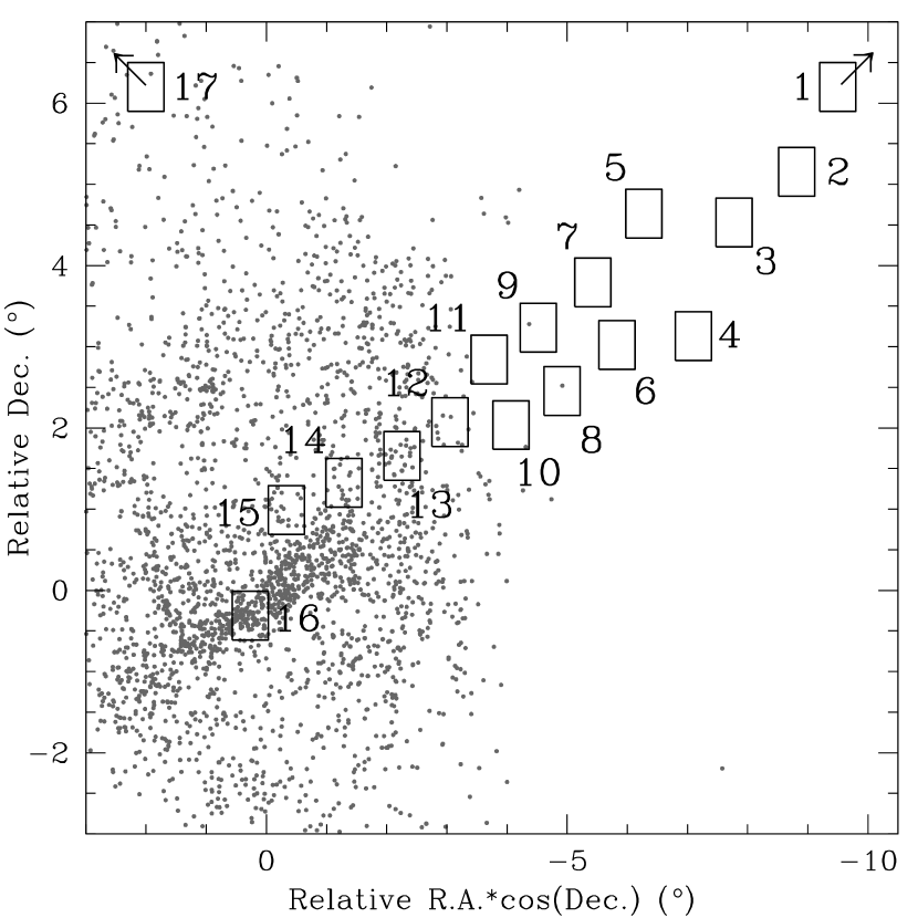
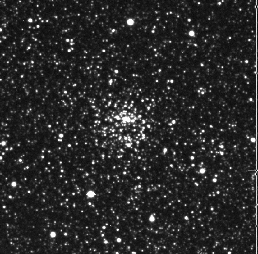
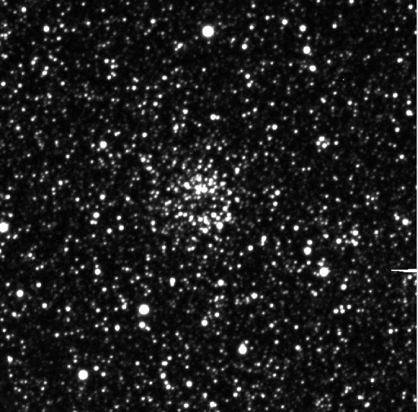
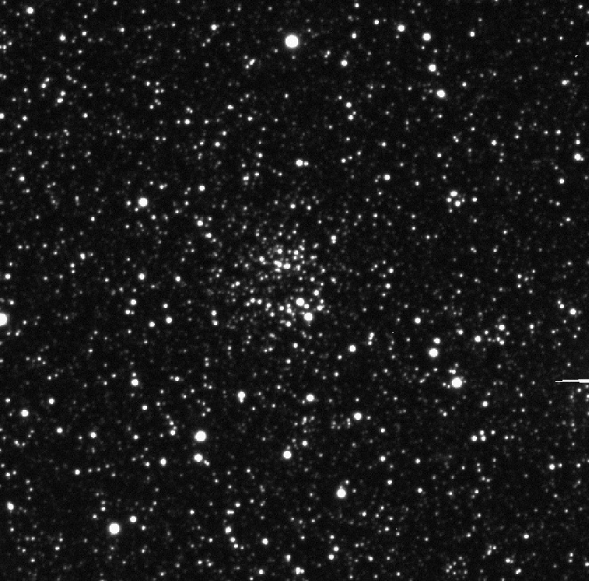
Figure 1: Top-left: Spatial distribution of the presently studied LMC star fields (thick black boxes). Star clusters catalogued by Bica et al. (2008) are also drawn (dots) for comparison purposes. To illustrate the data quality we include 4$\times$4 arcmin subsections of our $CMR$ images of Field 15, centred on field BRHT 34a,b in the bottom-left, top-right and bottom-right panels, respectively. North is up and East to the left. The full $CMR$ images of Field 15 (the most densely populated one, regardless Field 16 (Piatti, 2017a)), and those for Field 1 (the least populated one) are provided as supplementary material in the online version of the journal.

The data used in this work come from the Cerro-Tololo Inter-American Observatory (CTIO) programme 2008B-0296 (PI: Cole) focused on surveying the most metal-poor stars outside the Milky Way. We downloaded from the National Optical Astronomy Observatory (NOAO) Science Data Management (SDM) Archives Washington $CM$ and Kron-Cousins $R$ images obtained with the Mosaic II imager, an array of 8K$\times$8K CCDs covering a 36$\arcmin$$\times$36$\arcmin$ field, attached to the 4 m Blanco telescope. Table 1 presents the log of the observations, where the main astrometric and observational information is summarized. The whole survey comprises 17 different LMC fields as illustrated in Fig. 1.

As previously performed for similar data sets (e.g. Piatti et al., 2012; Piatti, 2012a, 2015, and references therein), we carried out the data processing and obtained the standardized photometry following the procedures documented by the NOAO Deep Wide Field Survey team (Jannuzi et al., 2003), and utilizing the mscred package in IRAF and the daophot/allstar suite of programs (Stetson et al., 1990). The raw images were first customized by performing overscan, trimming, bias subtraction and flat-field corrections. The applied zero and sky- and dome- flats come from properly combined individual ones. We also took advantage of $\sim$ 500 stars catalogued by the USNO to obtain an updated world coordinate system (WCS) with an rms error smaller than 0.4 arcsec in RA and DEC.

We measured nearly 270 independent magnitudes in the standard fields PG0321+051, SA 98 and SA 101 (Landolt, 1992; Geisler, 1996) – observed three times per night (Dec. 27 – 30, 2008) – using the apphot task within IRAF. These magnitudes were used to derive the coefficients to transform the instrumental $cmr$ system to the Washington $CMT_{1}$ system. We fitted the following expressions:

$$c=c_{1}+T_{1}+(C-T_{1})+c_{2}\times X_{C}+c_{3}\times(C-T_{1}),$$ (1)

$$m=m_{1}+T_{1}+(M-T_{1})+m_{2}\times X_{M}+m_{3}\times(M-T_{1}),$$ (2)

$$r={t_{1}}_{1}+T_{1}+{t_{1}}_{2}\times X_{T_{1}}+{t_{1}}_{3}\times(C-T_{1}),$$ (3)

where $c_{i}$, $m_{i}$ and ${t_{1}}_{i}$ ($i$ = 1, 2 and 3) are the fitted coefficients, and $X$ represents the effective airmass. Instrumental and standard magnitudes are distinguished by lowercase and capital letters, respectively. Note that eq. (3) involves $r$ magnitudes to derive $T_{1}$ magnitudes because the $R$ filter is the recommended substitute of the Washington $T_{1}$ filter (Geisler, 1996). The resultant transformation coefficients for each night, obtained with the fitparams task in IRAF, are shown in Table 2.

The stellar photometry for each single mosaic – produced by gathering all together the 8 CCDs using the updated WCS – was obtained after deriving the respective quadratically varying point-spread-function (PSF). Such a PSF was created by using two lists of stars, one with $\sim$ 1000 and another with the brightest $\sim$ 250 stars, both selected interactively. A preliminary PSF is obtained from the smallest sample, which is used to clean the largest PSF star sample. The procedure to derive PSF magnitudes of the stars identified in each field consisted in applying the resultant PSF to the single mosaic; then identifying new fainter stars in the output subtracted frame, and running again the allstar program for the enlarged sample of stars. We iterated this loop three times. Only objects with $\chi$ $<$ 2, photometric error less than 2$\sigma$ above the mean error at a given magnitude, roundness values between -0.5 and 0.5 and sharpness values between 0.2 and 1.0 were kept. Finally, we used eqs. (1) to (3) to standardize the PSF instrumental magnitudes and the daomatch and daomaster programs to put the stellar $CMT_{1}$ magnitudes of each field into a single file.

We estimated the errors of our photometry from artificial star tests carried out using the stand-alone addstar program in the daophot package Stetson et al. (1990) to add synthetic stars with Poisson noise, generated bearing in mind the colour and magnitude distributions of the stars in the cluster colour-magnitude diagrams (CMDs), as well as their radial stellar density profiles. We added $\sim$ 5$\%$ of the measured stars in order to produce a thousand synthetic images with similar stellar densities as observed. The synthetic images were used to obtain stellar PSF magnitudes as described above. Then, by comparing the output and the input magnitudes of the added stars we estimated the respective photometric errors. Fig. 2 illustrates the typical photometric errors with errorbars at the left margin the CMDs.

Table 1: Observations log of selected LMC star fields.

ID	R.A.(J2000.0)	Dec.(J2000.0)	filtersa			exposures			airmass			mean seeing
	(h m s)	($\degr$ $\arcmin$ $\arcsec$)				(sec)						($\arcsec$)
Field 1	01 09 34.28	-52 23 10.3	C	M	R	1$\times$150	1$\times$20	1$\times$15	1.22	1.22	1.23	1.2	1.1	1.1
Field 2	03 59 33.04	-64 19 29.3	C	M	R	1$\times$300	1$\times$60	1$\times$30	1.22	1-22	1.23	1.3	1.2	1.2
Field 3	04 07 30.02	-64 56 48.8	C	M	R	1$\times$420	1$\times$60	1$\times$30	1.22	1.22	1.23	1.0	1.0	1.0
Field 4	04 10 09.88	-66 20 58.6	C	M	R	1$\times$300	1$\times$60	1$\times$30	1.24	1.24	1.24	1.1	1.0	1.0
			C	M	R	1$\times$300	1$\times$45	1$\times$30	1.30	1.30	1.31	1.2	1.2	1.1
Field 5	04 21 53.04	-64 50 26.2	C	M	R	1$\times$300	1$\times$30	1$\times$20	1.29	1.30	1.29	1.3	1.2	1.2
Field 6	04 22 35.71	-66 27 25.9	–	M	R	–	1$\times$120	1$\times$30	–	1.24	1.24	–	1.0	1.0
Field 7	04 28 13.14	-65 41 13.6	–	M	R	–	1$\times$60	1$\times$30	–	1.24	1.24	–	1.1	1.1
Field 8	04 30 36.03	-67 01 26.0	C	–	R	1$\times$420	–	1$\times$30	1.25	–	1.25	1.2	–	1.1
Field 9	04 36 03.74	-66 14 30.8	–	M	R	–	1$\times$60	1$\times$30	–	1.34	1.34	–	1.0	1.0
Field 10	04 38 30.77	-67 26 30.8	–	M	R	–	1$\times$45	1$\times$20	–	1.55	1.51	–	1.2	1.2
Field 11	04 43 36.55	-66 38 12.1	–	M	R	–	1$\times$60	1$\times$30	–	1.27	1.28	–	1.2	1.2
Field 12	04 49 11.12	-67 24 22.0	–	M	R	–	1$\times$60	1$\times$30	–	1.29	1.29	–	1.1	1.1
Field 13	04 57 04.68	-67 49 17.4	–	M	R	–	1$\times$60	1$\times$30	–	1.63	1.64	–	1.1	1.1
Field 14	05 07 03.50	-68 09 19.1	–	M	R	–	1$\times$60	1$\times$30	–	1.45	1.44	–	1.1	1.0
Field 15	05 17 18.89	-68 29 14.6	C	M	R	1$\times$420	1$\times$60	1$\times$30	1.58	1.57	1.61	1.3	1.2	1.2
Field 16	05 24 04.21	-69 47 23.8	C	M	R	1$\times$420	1$\times$60	1$\times$30	1.34	1.34	1.31	1.2	1.2	1.2
Field 17	05 58 31.97	-48 38 32.5	C	M	R	1$\times$80	1$\times$20	1$\times$10	1.39	1.38	1.41	1.1	1.1	1.1

^a Note that the Kron-Counsins $R$ filter is the recommended substitute of the Washington $T_{1}$ filter (Geisler, 1996).

Table 2: Washington $CMT_{1}$ transformation ero point (1), extinction (2) and colour term (3) coefficients.

Date (UT)	$c_{1}$	$c_{2}$	$c_{3}$	rms
Dec. 27	0.149$\pm$0.013	0.280$\pm$0.010	-0.099$\pm$0.007	0.037
Dec. 28	0.033$\pm$0.017	0.292$\pm$0.011	-0.083$\pm$0.004	0.030
Dec. 29	0.030$\pm$0.019	0.283$\pm$0.130	-0.086$\pm$0.005	0.029
Dec. 30	0.016$\pm$0.015	0.289$\pm$0.009	-0.094$\pm$0.003	0.023
Date (UT)	$m_{1}$	$m_{2}$	$m_{3}$	rms
Dec. 27	-0.926$\pm$0.009	0.140$\pm$0.010	-0.246$\pm$0.012	0.016
Dec. 28	-0.999$\pm$0.014	0.132$\pm$0.009	-0.230$\pm$0.008	0.024
Dec. 29	-1.028$\pm$0.015	0.145$\pm$0.009	-0.240$\pm$0.008	0.022
Dec. 30	-1.034$\pm$0.013	0.139$\pm$0.008	-0.234$\pm$0.007	0.020
Date (UT)	${t_{1}}_{1}$	${t_{1}}_{2}$	${t_{1}}_{3}$	rms
Dec. 27	-0.605$\pm$0.010	0.080$\pm$0.010	-0.030$\pm$0.006	0.031
Dec. 28	-0.679$\pm$0.015	0.080$\pm$0.011	-0.018$\pm$0.003	0.021
Dec. 29	-0.665$\pm$0.019	0.071$\pm$0.013	-0.026$\pm$0.004	0.029
Dec. 30	-0.723$\pm$0.008	0.101$\pm$0.005	-0.025$\pm$0.002	0.013

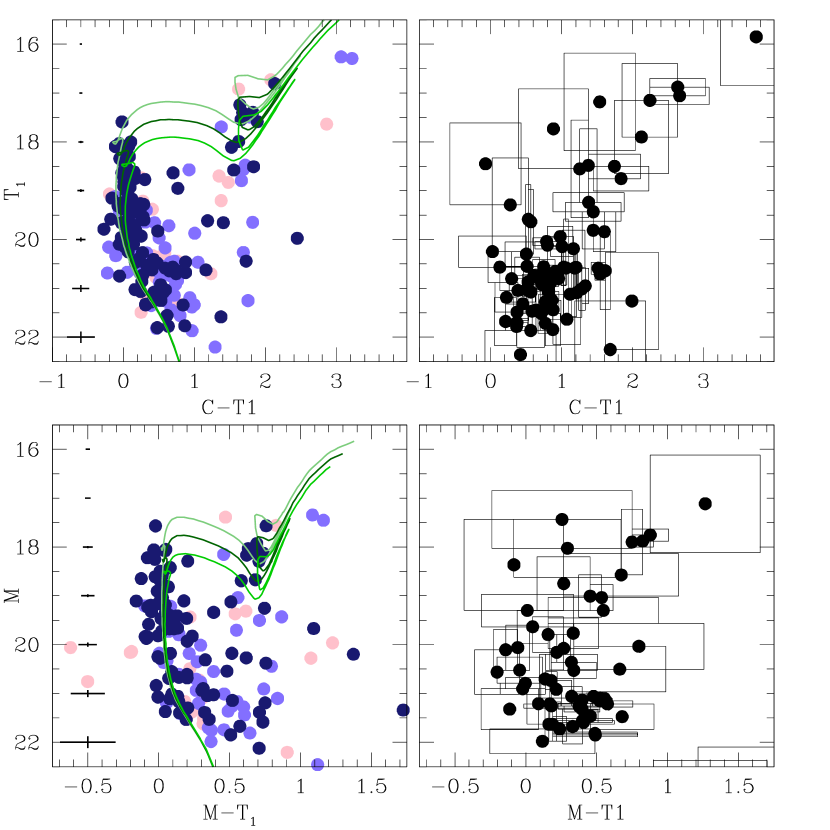
Figure 2: CMDs for stars in the field of KMHK 691 with typical photometric errors represented with errorbars at the left margin Colour-scaled symbols represent stars that statistically belong to the field ($P\leq$ 25%, pink), stars that might belong to either the field or the cluster ($P=$ 50%, light blue), and stars that predominantly populate the cluster region ($P\geq$ 75%, dark blue). Three isochrones from Bressan et al. (2012) for log($t$ yr^-1) = 8.5 (pale green), 8.6 (dark green), and 8.7 (medium green) and $Z$ = 0.006 are also superimposed. Right panels illustrate the definition of boxes in the field-star CMD.

3 The star cluster sample

Instead of using the up-to-date list of catalogued clusters, we decided to perform an homogeneous search over all observed LMC fields using the procedure developed in Piatti et al. (2016) and also successfully used elsewhere (e.g. Piatti, 2016, 2017b). Thus, we could not only recover the known clusters but also search for new ones, particularly extending to the fields beyond the LMC main body. For the sake of the reader we describe the steps followed: we started by using the daofind task within daophot to detect every stellar source in the deepest images. Then, we built continuous density distributions using two different Kernel Density Estimators (KDEs), namely, Gaussian and tophat, and a KDE bandwidth of 0.4 arcmin, that allowed us to extract the finest structures of them (e.g., smallest and/or less dense resolved clusters). Piatti et al. (2016) showed that the mean stellar cluster density as a function of cluster radius is a suitable diagnostic diagram to infer the appropriate bandwidth; the only free parameter while using KDE. Such a diagram shows the range of cluster sizes and their stellar densities, so that in order to detect the smallest clusters, a KDE bandwidth of the order of the diameter of the smallest clusters should be used. They showed that such a criterion allowed them to recover 100 per cent of the known clusters (see also, Piatti, 2017b, a). By using larger bandwidths, some small clusters could be missed.

To this purpose, we used the Python KDE routing within AstroML (Vanderplas et al., 2012, and reference therein for a detail description of the complete AstroML package and user’s manual), a machine learning and data mining for Astronomy package. AstroML is a Python module for machine learning and data mining built on numpy, scipy, scikit-learn, matplotlib, and astropy, and distributed under the 3-clause BSD license. It contains a growing library of statistical and machine learning routines for analysing astronomical data in Python, loaders for several open astronomical data sets, and a large suite of examples of analysing and visualizing astronomical datasets. The goal of AstroML is to provide a community repository for fast Python implementations of common tools and routines used for statistical data analysis in astronomy and astrophysics, to provide a uniform and easy-to-use interface to freely available astronomical data sets.

The second step consisted in deciding which of the total number of overdensities detected above are star cluster candidates. Here, we considered the height (i.e., the peak in stellar density of an overdensity) relative to the local background and a cut-off density of 1.5 times the local background dispersion above the mean background value, to increase the chance of identifying star cluster candidates (Piatti et al., 2016). As far as we are aware, we used the most suitable values in order to identify star cluster candidates, since we chose a bandwidth value of the order of the diameter of the smallest known clusters. Indeed, we identified all the previously known star clusters and detected some new ones. By using smallest bandwidths, the same number of true clusters is recovered. The appropriate height relative to the local background was adopted by looking at the stellar density versus local background plot for a grid of points distributed throughout the field. Piatti et al. (2016) assumed similar conditions while searching for new star clusters in the densest and highest reddened region ($\sim$ 0.4 deg²) of the Small Magellanic Cloud (SMC) bar, and identified the 68 catalogued star clusters in Bica et al. (2008, hereafter B08) and 38 new ones. Our resulting numbers of star cluster candidates are listed in Table 3.

In order to decontaminate the star cluster candidate CMDs from field stars we applied a procedure developed by Piatti & Bica (2012), and successfully used elsewhere (e.g. Piatti, 2014; Piatti et al., 2015a; Piatti et al., 2015b; Piatti & Bastian, 2016, and references therein). Briefly, the field star cleaning relies on the subtraction of different previously defined field-star CMDs to the cluster CMD. We used a total of four different field-star CMDs of regions located to the north, east, south and west from the cluster centre, respectively. The field regions have the same area as that used for the cluster, i.e., of a circle of radius three times as big as the cluster radii given by B08. For each field-star CMD we produced a number of boxes – as many as stars in the field-star CMD – that are centred at the magnitudes and colours of the stars and that have sizes as large as their corners coincide with the position of their closest star; magnitude and colour sides are adjusted independently. Right panels of Fig. 2 illustrate the definition of the boxes in the field-star CMD. We then placed those boxes on the cluster CMD and eliminated one star per box, choosing the closest one to its centre that lies inside it. We repeated the procedure for all the four field-star CMDs. The method has proved to be powerful to effectively reproduce the local field star signature in terms of stellar density, luminosity function and colour distribution. Here we used four field star CMDs constructed from stars located around the clusters and with areas equal to the circular area used for the cluster region.

Photometric membership probabilities were then assigned on the basis of the number of times a star in the cluster CMD was kept unsubtracted, once the four independent cleanings were executed. If a star appeared once in the four cleaned CMDs (the same cluster CMD cleaned from four different field-star CMDs), we gave it a membership probability $P\leq$ 25 per cent. If a star appeared twice, then it was given a probability $P=$ 50 per cent; and for more than twice, $P\geq$ 75 per cent. Because of the statistical subtraction process, a small amount of residuals can be arise, depending on the particular features of the considered star field (stellar density variability, etc). We finally discarded two objects known in the literature as [HS66] 197 and KMHK309n, whose cleaned CMDs do not show any detectable trace of star cluster sequences. Table 3 presents the statistics of confirmed star cluster per field, while Figure 2 illustrates the performance of the cleaning procedure for KMHK 691. The individual photometric catalogues for the confirmed clusters are provided in the online version of the journal. The columns of each catalogue successively lists the star ID, the R.A. and Dec., the X and Y coordinates (in pixels), the magnitude and error in $C$, $M$ and $T_{1}$, respectively, $\chi$ and sharpness, and the photometric membership probability ($P$). The latter is encoded with numbers 1, 2, 3 and 4 to represent probabilities of 25, 50, 75 and 100 per cent, respectively. A portion of the photometric catalogue of KMHK 685 is shown in the Appendix for guidance regarding their form and content.

As far as we are aware, the final cluster sample is statistically complete, if we bear in mind the depth of our photometry and the distance of the LMC. Indeed, young star clusters are distinguished in the CMDs by their bright MSs, while intermediate-age clusters have main-sequence turnoffs (MSTOs) that decrease in brightness as they become older. The oldest intermediate-age clusters are $\sim$ 2.5 Gyr old (Piatti & Geisler, 2013), which in turn implies a MSTO at $T_{1}$ $\sim$ (20.5 $\pm$ 0.15) mag, assuming an average depth of 3.44$\pm$1.16 kpc (Subramanian & Subramaniam, 2009). This magnitude is brighter than our limiting magnitude, so that we were able to detect any star cluster based on counts of its brightest stars all the way down to its MSTO. The exception to this would be genuinely old globular clusters (log($t$ yr^-1) $\sim$ 10), which have fainter MSTOs.

Nevertheless, we performed a matching between the catalogued clusters by B08 and Glatt et al. (2010) and our final cluster sample. We confirmed that every object in our sample is in B08/Glatt et al. (2010), except two new cluster candidates, one reported by Piatti (2017a) and another one with coordinates R.A.= 72$\degr$.579697, DEC.= -67$\degr$.703239 (J2000.0). The latter was not resolved by the SIMBAD astronomical data base either. The very few new star cluster candidates detected would not appear to support some recent outcomes that have shown that there are still a substantial number of extreme low luminosity stellar clusters undetected in the wider Magellanic System periphery and the Milky Way halo (Kim et al., 2015; Pieres et al., 2016; Martin et al., 2016). These latter results are based on deep images obtained with the Dark Energy Camera (DECam) at the CTIO 4 m Blanco telescope (see Valdes et al., 2014), and the discovery of some few faint extended stellar objects led to speculate on the possible existence of larger amounts of star clusters. Furthermore, streams of gas and stars that might harbour stellar clusters have also been detected (Mackey et al., 2016; Belokurov et al., 2017; Deason et al., 2017), but a complete search for new clusters in the DECam fields is still pending. Conversely, our findings agrees well with other recent results obtained by Piatti (2017b), who also concluded on low chances of detecting a significant number of stellar clusters there from DECam deep images.

We also found that several B08’s clusters were not identified by our procedure; one of them (H88 34) because it falls on a Mosaic II image gap. The remaining objects could not be recognised when visually inspecting the $C$, $M$ and $T_{1}$ images either, because the distribution of stars in their respective fields do not resemble that of a stellar aggregate. We consider them as probable non-genuine star clusters. They are: KMHK 125 in Field 12; BSDL 616, 631, 661, 677, [GKK2003] O219, O222, KMHK  609 and OGLE-CL LMC 122 in Field 14; BSDL  962, 1157, 1294, [HS66] 231 and KMHK759 in Field 15. For Field 16, we refer the reader to Piatti (2017a), who also discusses the origin of those asterisms, namely, the lower spatial resolution and magnitude limit (see also, Piatti & Bica, 2012; Piatti, 2014).

Table 3: Statistics of star clusters in the presently studied LMC star fields.

ID	detected star	confirmed	B08 unlikely
	cluster candidates	star clusters	star clusters
Field 1	–	–	–
Field 2	–	–	–
Field 3	–	–	–
Field 4	–	–	–
Field 5	–	–	–
Field 6	–	–	–
Field 7	–	–	–
Field 8	1	1	–
Field 9	1	1	–
Field 10	1	1	–
Field 11	1	1	–
Field 12	11	11	1
Field 13	24a	23	–
Field 14	17	17	8
Field 15	22	21	5
Field 16b	73	70	38
Field 17	–	–	–

^a H88 34 was not detected, because it falls on an image gap.

^b values taken from Piatti (2017a).

4 Star cluster age estimates

In order to estimate the ages of the studied clusters, we used the theoretical isochrones of Bressan et al. (2012) to match their CMDs built from stars with membership probabilities higher than 50 per cent. Hence we assigned to a cluster an age equal to the isochrone’s age which best resembles the cluster CMD features. Because of the LMC distance (49.90${}^{-2.04}_{+2.10}$ kpc, de Grijs et al., 2014) and its depth (3.44$\pm$1.16 kpc, Subramanian & Subramaniam, 2009), the difference in the cluster distance moduli could be as large as $\Delta$$(m-M)_{o}$ $\sim$ 0.3 mag. This difference is similar to that we would get at the MSTO $T_{1}$ mag when matching theoretical isochrones to the cluster CMDs, aiming at reproducing the observed dispersion (see Fig. 2). The inclination of the LMC disc to the line of sight could also contribute to distance differences, but the position angle of the observed fields is near to the line of nodes (e.g. van der Marel, 2001), so the distance change is unlikely to be large compared to its uncertainty. For this reason, we adopted a mean distance modulus of $(m-M)_{o}$ = 18.49 mag for all the clusters.

We also used isochrones for Z = 0.006 ([Fe/H] = $-$0.4 dex), which corresponds to the mean LMC metal content during the last $\sim$ 2-3 Gyr. Note that the age-metallicity relationship for LMC clusters derived by Piatti & Geisler (2013) shows that the LMC chemical evolution has mostly taken place within a constrained metallicity range during this period ([Fe/H] $\approx$ -0.7 dex to -0.2 dex) and differences in theoretical isochrones, particularly along the main sequence (MS), are negligible compared to the observed dispersion. We made one exception in the employment of the isochrones for the old globular cluster NGC 1786, that lies in Field 13, and for which we adopted [Fe/H] = $-$2 dex (Brocato et al., 1996; Carretta et al., 2000).

Since the reddening is expected to vary across the surveyed regions, we estimated $E(V-I)$ colour excesses from the Magellanic Clouds (MCs) extinction values based on the red clump (RC) and RR Lyrae stellar photometry provided by the Optical Gravitational Lens Experiment (Udalski, 2003, OGLE III) collaboration, as described in Haschke et al. (2011). In matching the isochrones, we started by adopting those $E(V-I)$ values, combined with the equations $E(V-I)$/$E(B-V)$ = 1.25, $A_{V}$/$E(B-V)$ = 3.1 (Cardelli et al., 1989), $E(C-T_{1})$/$E(B-V)$ = 1.97 and $A_{T_{1}}$/$E(B-V)$ = 2.62 (Geisler, 1996), and the adopted mean LMC distance modulus, to properly shift the theoretical isochrones in $T_{1}$ and $M$ magnitudes and $C-T_{1}$ and $M-T_{1}$ colours. When overplotting the theoretical isochrones, we used the shape of the MS, its curvature, the relative distance between the RC and the MSTO in magnitude and colour, separately, among others, as reddening- and distance-free features to choose the isochrone which best reproduce them. We estimated the overall age uncertainty associated to the observed dispersion in magnitude in the cluster CMDs to be $\Delta$log($t$ yr^-1) = $\pm$0.10. Notice that the magnitude of the MSTO is age-dependent and that the position of the red clump also constrains the age range. Fig. 2 illustrates the performance of the isochrone matching for two different CMDs, while Table 4 lists the derived $E(V-I)$ colour excesses and ages.

We previously studied many of these clusters from different Washington photometry data sets, while some others were analysed by Glatt et al. (2010) as part of the Magellanic Cloud Photometric Surveys Zaritsky et al. (MCPS 2002). The result of the comparison between them is depicted in Fig. 3, while Table 3 lists the values and references taken from the literature. As can be seen, the agreement is fairly good, except in the case of some clusters studied by Glatt et al. (blue filled squares). We recall that they did not perform any decontamination of field stars from the cluster CMDs and that the MCPS reaches MSTOs of clusters younger than $\sim$ 1 Gyr. It is possible that the lack of cleaned CMDs and their shallower photometry did not allow them to achieve more reliable age estimates. The very good agreement with previous Washington photometry studies provides additional support to the nearly 30 per cent of the clusters studied here for which, as far as we are aware, their ages are estimated for the first time.

Table 4: Fundamental properties of the star cluster sample.

	Cluster name	$E(V-I)$	log($t$ yr-1)		Ref.
			this work	literature
Field 8	KMHK 5	0.05	9.10$\pm$0.10	9.20$\pm$0.10	1
Field 9	NGC 1644	0.05	9.10$\pm$0.10	9.15$\pm$0.15	1
Field 10	KMHK 11	0.05	9.30$\pm$0.10
Field 11	KMHK 72	0.05	8.90$\pm$0.10	8.60$\pm$0.10	4
Field 12	BSDL 21	0.09	9.10$\pm$0.10
	BSDL 38	0.06	8.60$\pm$0.10	8.70$\pm$0.20	2
	BSDL 75	0.09	8.90$\pm$0.10
	BSDL 77	0.06	8.90$\pm$0.10	8.90$\pm$0.10	4
	BSDL 87	0.05	7.80$\pm$0.10	7.90$\pm$0.10	5
	KMHK 84	0.08	9.10$\pm$0.10	9.15$\pm$0.05	1
	KMHK 95	0.07	8.60$\pm$0.10	8.55$\pm$0.10	4
	KMHK 112	0.06	9.20$\pm$0.10	9.10$\pm$0.05	1
	KMHK 148	0.05	9.10$\pm$0.10	8.60$\pm$0.10	3
	KMHK 158	0.06	7.30$\pm$0.10	7.80$\pm$0.10	5
	new cluster	0.06	7.30$\pm$0.10
Field 13	BRHT 45a	0.09	8.20$\pm$0.10	8.10$\pm$0.10	4
	BRHT 45b	0.09	7.90$\pm$0.10	7.90$\pm$0.10	5
	BRHT 62a	0.05	8.40$\pm$0.10	8.60$\pm$0.10	5
	BRHT 62b	0.05	8.20$\pm$0.10
	BSDL 341	0.07	8.60$\pm$0.10	8.45$\pm$0.10	4
	H88 25	0.07	9.10$\pm$0.10	9.20$\pm$0.05	1
	H88 26	0.06	8.90$\pm$0.10	8.90$\pm$0.10	3
	H88 32	0.07	8.60$\pm$0.10	8.40$\pm$0.10	5
	H88 40	0.08	9.00$\pm$0.10	8.85$\pm$0.10	3
	H88 52	0.09	9.00$\pm$0.10	9.05$\pm$0.10	4
	H88 53	0.09	8.40$\pm$0.10	8.20$\pm$0.40	2
	H88 66	0.07	8.80$\pm$0.10
	H88 67	0.07	9.00$\pm$0.10	9.15$\pm$0.10	1
	H88 78	0.09	8.80$\pm$0.10
	H88 79	0.08	9.25$\pm$0.10	9.20$\pm$0.05	1
	KMHK 286	0.09	8.50$\pm$0.10	8.35$\pm$0.20	4
	KMHK 309s	0.09	7.80$\pm$0.10	7.90$\pm$0.10	5
	KMHK 333	0.09	8.80$\pm$0.10	8.40$\pm$0.40	2
	KMHK 348	0.08	9.00$\pm$0.10	9.15$\pm$0.05	1
	KMHK 367	0.08	8.80$\pm$0.10	8.70$\pm$0.10	3
	KMHK 390	0.07	8.80$\pm$0.10	8.70$\pm$0.10	3
	NGC 1764	0.08	8.00$\pm$0.10	7.90$\pm$0.10	5
	NGC 1786	0.06	10.10$\pm$0.10	10.10	6,7
Field 14	BSDL 527	0.04	9.25$\pm$0.10	9.15$\pm$0.05	1
	BSDL 716	0.06	8.70$\pm$0.10	8.60$\pm$0.10	3
	BRHT 29a	0.07	8.60$\pm$0.10	8.50$\pm$0.10	4
	BRHT 29b	0.07	7.80$\pm$0.10	7.90$\pm$0.10	4
	[HS66] 131	0.09	9.00$\pm$0.10	9.15$\pm$0.10	4
	KMHK 505	0.06	8.70$\pm$0.10	8.75$\pm$0.10	4
	KMHK 506	0.04	8.90$\pm$0.10	8.75$\pm$0.05	3
	KMHK 531	0.05	8.40$\pm$0.10	8.30$\pm$0.10	5
	KMHK 533	0.04	9.20$\pm$0.10	9.10$\pm$0.05	1
	KMHK 536	0.06	8.50$\pm$0.10	8.55$\pm$0.10	4
	KMHK 549	0.06	8.70$\pm$0.10
	KMHK 554	0.06	8.00$\pm$0.10
	KMHK 560	0.04	9.00$\pm$0.10	9.15$\pm$0.05	1
	KMHK 586	0.05	9.10$\pm$0.10	9.25$\pm$0.05	1
	NGC 1829	0.04	7.90$\pm$0.10
	NGC 1838	0.06	8.50$\pm$0.10	8.00$\pm$0.20	2
	ZHT AN 8	0.07	9.10$\pm$0.10
Field 15	BRHT 34a	0.11	8.65$\pm$0.10	8.30$\pm$0.20	2
	BRHT 34b	0.11	8.50$\pm$0.10	8.45$\pm$0.20	2
	BSDL 1035	0.10	8.50$\pm$0.10	8.70$\pm$0.10	3
	BSDL 1046	0.08	9.20$\pm$0.10	8.60$\pm$0.40	2
	BSDL 1139	0.10	8.55$\pm$0.10
	BSDL 1141	0.11	8.30$\pm$0.10
	BSDL 1152	0.10	9.10$\pm$0.10	8.40$\pm$0.20	2
	BSDL 1161	0.10	9.00$\pm$0.10
	[HS66] 221	0.08	8.40$\pm$0.10	8.20$\pm$0.20	2

Table 4: continued.

	Cluster name	$E(V-I)$	log($t$ yr-1)		Ref.
			this work	literature
Field 15	ESO 56-SC 91	0.10	8.50$\pm$0.10
	KMHK 685	0.11	9.30$\pm$0.10	8.70$\pm$0.40	2
	KMHK 691	0.13	8.60$\pm$0.10	8.40$\pm$0.20	2
	KMHK 727	0.10	9.20$\pm$0.10	9.20$\pm$0.10	8
	KMHK 753	0.08	8.80$\pm$0.10
	KMHK 775	0.11	8.00$\pm$0.10	7.90$\pm$0.20	2
	KMHK 784	0.14	8.80$\pm$0.10
	KMHK 794	0.09	7.80$\pm$0.10
	[SL63] 327	0.07	8.40$\pm$0.10
	[SL63] 332	0.08	7.90$\pm$0.10	8.00$\pm$0.40	2
	[SL63] 351	0.13	8.70$\pm$0.10	8.65$\pm$0.05	3
	[SL63] 370	0.10	9.00$\pm$0.10

Ref.: (1) Piatti (2011); (2) Glatt et al. (2010); (3) Piatti (2012b); (4) Choudhury et al. (2015); (5) Piatti (2014); (6) Brocato et al. (1996); (7) Carretta et al. (2000); (8) Piatti et al. (2009).

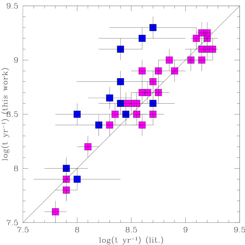
Figure 3: Comparison between ages taken from the literature and those estimated in this work. Blue filled squares refer to clusters with age estimated by Glatt et al. (2010).

5 analysis

In order to study the cluster formation history along the minor axis of the LMC, we constructed star cluster frequencies (CFs), defined as the number of clusters per age unit as a function of age. CFs have the advantage that they do not depend on the age interval, so that number of clusters at different ages can be compared. We built CFs for Fields 12 to 16, which are those that contain more than one cluster. Each CF was normalized to the respective total number of clusters for comparison purposes. From these CFs we compared the cluster formation activity in different epochs of the galaxy lifetime for a particular field, and between different LMC fields as well.

CFs were built assigning to each cluster age a Gaussian distribution centred on the mean cluster age and with FWHM twice as big as the age uncertainty. Thus we dodge constructing age histograms that depend on the bin size and the end points of bins. Moreover, since the age uncertainties can be larger than the size of the age bins, a cluster can actually reside in one of a few adjacent age bins. We considered this effect while building an intrinsic CF. We added all the Gaussian distributions and then computed the fraction of them that fall in different age intervals ($\Delta$(log($t$ yr^-1)) = 0.1). The result of summing the contribution of all Gaussian distributions for each observed field is depicted in Fig. 4.

At first glance, the oldest clusters turned out to be as old as log($t$ yr^-1) $\sim$ 9.3, in good agreement with the age range of most of the LMC clusters (log($t$ yr^-1) $\la$ 9.40, Piatti & Geisler, 2013, see their figure 6), with the exception of ESO 121-SC-03 (log($t$ yr^-1) $\sim$ 9.92) and 15 old globular clusters (log($t$ yr^-1) $\sim$ 10.1). From log($t$ yr^-1) $\sim$ 9.3 until $\sim$ 8.5 each region has undergone a relatively similar increasing, nearly smooth, cluster formation activity, with two exceptions: Field 12 (located near the edge of the LMC main body), which shows a slightly more interrupted cluster formation, and Field 16 (located nearly at the LMC centre), for which clusters have later started to be formed (log($t$ yr^-1) $\sim$ 8.9). Both pictures tell us about a particular spatial-age dependent scenario, in which clusters started to be formed mostly throughout the LMC main body, except in the very innermost bar, and that the gas out of which they formed was exhausted outside-in. The outside-in formation scenario has been proposed previously by Gallart et al. (2008); Piatti et al. (2009); Meschin et al. (2014), among others.

The uncertain process of cluster disruption in the LMC tidal field may complicate the simplest interpretation of the spatial patterns of cluster frequency versus age. As noted by Lamers et al. (2005), the characteristic cluster destruction timescale t_d is a strong function of the ambient field density, with t${}_{d}\propto\rho^{-1/2}$ in a typical model of the tidal disruption process. Since the field density varies dramatically across Fields 16 to 12, one might expect the age distribution to be steeper in the inner fields. However, all five fields have roughly similar CF vs. age slopes (to within significant scatter). It is suggestive that Field 16 shows a steep decline of the CF at younger ages than the other four fields, but not conclusive based on these data. In this context, it is worth noting that the cluster destruction timescale in the LMC as a whole has been constrained to be longer than $\approx$1 Gyr (e.g., Parmentier & de Grijs, 2008).

The process of cluster formation apparently entered a quiescent stage during the period log($t$ yr^-1) $\sim$ 8.0 – 8.3 for most of the studied fields, while in the innermost bar region (Field 16) it reached its highest formation activity, ended at log($t$ yr^-1) $\sim$ 8.0. Soon after (log($t$ yr^-1) $\sim$ 7.8–7.9), the regions where cluster formation had ceased or gone to a quiescent stage, experienced a sudden episode of cluster formation activity that notably continues until log($t$ yr^-1) $\sim$ 7.3 in the outermost one (Field 12), although with interrupted short periods, and has been mirrored in the innermost one, Field 16.

Besla et al. (2007) and Kallivayalil et al. (2013) suggested that the first infall of the LMC to the Milky Way (MW) took place at log($t$ yr^-1) $\sim$ 7.8, just close to the observed bursting cluster formation of Fig. 4. If such a burst were associated with this close passage of the LMC, then we should expect that some amount of gas to form young clusters reached the outermost western regions of the galaxy. Note that only Field 12 shows a roughly continuous cluster formation activity since log($t$ yr^-1) $\sim$ 7.9. Recently, Salem et al. (2015) and Indu & Subramaniam (2015) have suggested from observations and modelling of H I spatial and velocity distributions, that the outer regions of the LMC were disturbed by ram pressure effects due to the motion of the LMC in the MW halo. Particularly, Salem et al. (2015) found evidence that the LMC’s gaseous disc has recently experienced ram pressure stripping, with a truncated gas profile along the windward leading edge of the LMC disc. This means that some amount of gas could travel in the opposite direction to the LMC motion, and thus could contribute with material for the cluster formation in the western-outermost part of the galaxy (see their figure 17). Similarly, Indu & Subramaniam (2015) suggested possible outflows from the western LMC disc which could be due to ram pressure. From these results, we speculate here with the possibility that the recent star formation activity observed in the studied field could have triggered by tidal interaction of the LMC during its first passage close to the MW.

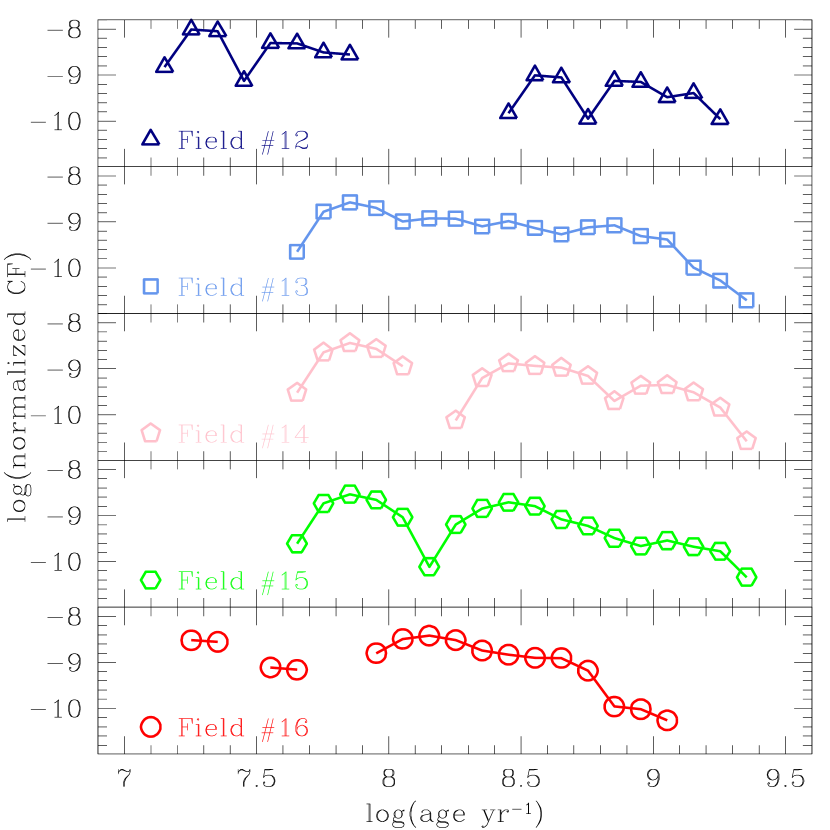
Figure 4: Normalized CFs of the observed LMC fields (see Fig. 1) plotted with different symbols as indicated in the bottom-left margin. The age intervals without clusters are distinguished as disconnected pair of points. Every CF has been divided (normalized) by the total number of clusters of the corresponding field, for comparison purposes.

6 Conclusions

In this work we analysed Washington $CMT_{1}$ photometry of star clusters located along the minor axis of the LMC. We covered a wide baseline in deprojected distances, from the very optical LMC centre up to $\sim$ 39 degrees outwards to the North-West.

We first performed an homogeneous search for star clusters in the 17 36$\arcmin$$\times$36$\arcmin$ studied fields using Gaussian and tophat KDEs with a bandwidth of 0.4 arcmin to produce continuous stellar density distributions, from which we identified stellar overdensities. For each of the detected cluster candidates we built CMDs statistically cleaned from field star contamination. The employed cleaning technique makes use of variable cells that allows us to reproduce the field star CMD as closely as possible. As a result, we confirmed the physical reality of 146 star clusters located in the LMC main body – two of them identified for the first time –, and concluded that an overall $\sim$ 30 per cent of catalogued clusters in the surveyed regions are non-possible physical systems. We did not find any new cluster candidate in the outskirts of the LMC (deprojected distance $\ga$ 8 degrees), in very good agreement with a recent search for new clusters performed on the SMASH survey data base across the Magellanic System Piatti (2017b).

The confirmed clusters comprise a complete sample, since we were able to detect any star cluster with stars from its brightest limit down to its MSTO. From matching theoretical isochrones to the cleaned cluster CMDs we estimated ages taking into account the LMC mean distance modulus, the present day metallicity and the individual star cluster colour excesses. As far as we are aware, these are the first age estimates based on resolved stellar photometry for nearly 30 per cent of the cluster sample. For the remaining clusters we found an excellent agreement between ages estimated previously, most of them from Washington $CT_{1}$ photometry, and our derived values. The derived ages are in the age range 7.2 < log($t$ yr^-1) $\leq$ 9.4, in addition to the old globular cluster NGC 1786.

Finally, we constructed CFs for each region with the aim of studying the cluster formation history along the minor axis of the LMC. We confirmed that there exists a age-spatial dependence of the cluster formation activity, in the sense that clusters in the innermost bar region started to be formed later (log($t$ yr^-1) $\sim$ 8.9) than those in more outlying regions (log($t$ yr^-1) $\sim$ 9.3), which reinforces previously proposed outside-in formation scenarios. Furthermore, when the cluster formation apparently entered a quiescent regime in most of the studied regions (log($t$ yr^-1) $\sim$ 8.0 –8.3), the innermost bar experienced its highest cluster formation activity. Later on, the outer studied fields show a sudden episode of cluster formation (log($t$ yr^-1) $\sim$ 7.8-7.9), that continued until log($t$ yr^-1) $\sim$ 7.3 only in the outermost LMC region, and had its mirrored event in the innermost bar region. These outcomes could be the first evidence from the study of star clusters that the first passage of the LMC by the Milky Way has triggered cluster formation due to the ram pressure of MW halo gas.

Appendix A Supplementary material provided online.

Table 5: Photometric catalogue of stars measured in the field of KMHK 685. Only a portion is shown here for guidance regarding its form and content. The whole content is available online. Photometric catalogues for all clusters in Table 4 are also available online.

ID	R.A.	Dec.	X	Y	$C$	$\sigma C$	$M$	$\sigma M$	$T_{1}$	$\sigma T_{1}$	$\chi$	sharpness	membership
	(hh:mm:ss)	($\degr$:$\arcmin$:$\arcsec$)	(pixels)	(pixels)	(mag)	(mag)	(mag)	(mag)	(mag)	(mag)
-	-	-	-	-	-	-	-	-	-	-	-	-	-
145713	05:14:46.694	-68:20:50.40	6090.440	973.777	20.4462	0.0290	20.1651	0.0410	19.9675	0.0420	0.7520	0.2670	2
145718	05:14:50.961	-68:20:50.26	6090.743	1063.417	20.3552	0.0160	19.4249	0.0190	18.8257	0.0150	1.1603	0.3897	2
145730	05:14:56.604	-68:20:50.04	6091.319	1181.795	20.3062	0.0320	19.3921	0.0120	18.8368	0.0200	0.9477	0.0187	1
-	-	-	-	-	-	-	-	-	-	-	-	-	-

References

- Bekki & Chiba (2005) Bekki K., Chiba M., 2005, MNRAS, 356, 680
- Bekki et al. (2004) Bekki K., Couch W. J., Beasley M. A., Forbes D. A., Chiba M., Da Costa G. S., 2004, ApJ, 610, L93
- Belokurov et al. (2017) Belokurov V., Erkal D., Deason A. J., Koposov S. E., De Angeli F., Evans D. W., Fraternali F., Mackey D., 2017, MNRAS, 466, 4711
- Besla et al. (2007) Besla G., Kallivayalil N., Hernquist L., Robertson B., Cox T. J., van der Marel R. P., Alcock C., 2007, ApJ, 668, 949
- Besla et al. (2016) Besla G., Martínez-Delgado D., van der Marel R. P., Beletsky Y., Seibert M., Schlafly E. F., Grebel E. K., Neyer F., 2016, ApJ, 825, 20
- Bica et al. (2008) Bica E., Bonatto C., Dutra C. M., Santos J. F. C., 2008, MNRAS, 389, 678
- Bressan et al. (2012) Bressan A., Marigo P., Girardi L., Salasnich B., Dal Cero C., Rubele S., Nanni A., 2012, MNRAS, 427, 127
- Brocato et al. (1996) Brocato E., Castellani V., Ferraro F. R., Piersimoni A. M., Testa V., 1996, MNRAS, 282, 614
- Cardelli et al. (1989) Cardelli J. A., Clayton G. C., Mathis J. S., 1989, ApJ, 345, 245
- Carretta et al. (2000) Carretta E., Gratton R. G., Clementini G., Fusi Pecci F., 2000, ApJ, 533, 215
- Choudhury et al. (2015) Choudhury S., Subramaniam A., Piatti A. E., 2015, AJ, 149, 52
- Da Costa (1991) Da Costa G. S., 1991, in Haynes R., Milne D., eds, IAU Symposium Vol. 148, The Magellanic Clouds. p. 183
- Deason et al. (2017) Deason A. J., Belokurov V., Erkal D., Koposov S. E., Mackey D., 2017, MNRAS, 467, 2636
- Efremov & Elmegreen (1998) Efremov Y. N., Elmegreen B. G., 1998, MNRAS, 299, 588
- Frogel et al. (1990) Frogel J. A., Mould J., Blanco V. M., 1990, ApJ, 352, 96
- Gallart et al. (2008) Gallart C., Stetson P. B., Meschin I. P., Pont F., Hardy E., 2008, ApJ, 682, L89
- Geha et al. (1998) Geha M. C., et al., 1998, AJ, 115, 1045
- Geisler (1996) Geisler D., 1996, AJ, 111, 480
- Glatt et al. (2010) Glatt K., Grebel E. K., Koch A., 2010, A&A, 517, A50
- Harris & Zaritsky (2009) Harris J., Zaritsky D., 2009, AJ, 138, 1243
- Haschke et al. (2011) Haschke R., Grebel E. K., Duffau S., 2011, AJ, 141, 158
- Hodge (1960) Hodge P. W., 1960, ApJ, 132, 351
- Hodge (1961) Hodge P. W., 1961, ApJ, 133, 413
- Indu & Subramaniam (2015) Indu G., Subramaniam A., 2015, A&A, 573, A136
- Jannuzi et al. (2003) Jannuzi B. T., Claver J., Valdes F., 2003, The NOAO Deep Wide Field Survey MOSAIC Data Reductions, http://www.noao.edu/noao/noaodeep/ReductionOpt/frames.html
- Kallivayalil et al. (2013) Kallivayalil N., van der Marel R. P., Besla G., Anderson J., Alcock C., 2013, ApJ, 764, 161
- Kim et al. (2015) Kim D., Jerjen H., Mackey D., Da Costa G. S., Milone A. P., 2015, ApJ, 804, L44
- Lamers et al. (2005) Lamers H. J. G. L. M., Gieles M., Portegies Zwart S. F., 2005, A&A, 429, 173
- Landolt (1992) Landolt A. U., 1992, AJ, 104, 340
- Mackey et al. (2016) Mackey A. D., Koposov S. E., Erkal D., Belokurov V., Da Costa G. S., Gómez F. A., 2016, MNRAS, 459, 239
- Martin et al. (2016) Martin N. F., et al., 2016, ApJ, 830, L10
- Meschin et al. (2014) Meschin I., Gallart C., Aparicio A., Hidalgo S. L., Monelli M., Stetson P. B., Carrera R., 2014, MNRAS, 438, 1067
- Parmentier & de Grijs (2008) Parmentier G., de Grijs R., 2008, MNRAS, 383, 1103
- Piatti (2011) Piatti A. E., 2011, MNRAS, 418, L40
- Piatti (2012a) Piatti A. E., 2012a, MNRAS, 422, 1109
- Piatti (2012b) Piatti A. E., 2012b, A&A, 540, A58
- Piatti (2014) Piatti A. E., 2014, MNRAS, 440, 3091
- Piatti (2015) Piatti A. E., 2015, MNRAS, 451, 3219
- Piatti (2016) Piatti A. E., 2016, MNRAS,
- Piatti (2017a) Piatti A. E., 2017a, preprint, (arXiv:1707.07032)
- Piatti (2017b) Piatti A. E., 2017b, ApJ, 834, L14
- Piatti & Bastian (2016) Piatti A. E., Bastian N., 2016, A&A, 590, A50
- Piatti & Bica (2012) Piatti A. E., Bica E., 2012, MNRAS, 425, 3085
- Piatti & Cole (2017) Piatti A. E., Cole A., 2017, MNRAS, 470, L77
- Piatti & Geisler (2013) Piatti A. E., Geisler D., 2013, AJ, 145, 17
- Piatti et al. (2009) Piatti A. E., Geisler D., Sarajedini A., Gallart C., 2009, A&A, 501, 585
- Piatti et al. (2012) Piatti A. E., Geisler D., Mateluna R., 2012, AJ, 144, 100
- Piatti et al. (2015a) Piatti A. E., de Grijs R., Rubele S., Cioni M.-R. L., Ripepi V., Kerber L., 2015a, MNRAS, 450, 552
- Piatti et al. (2015b) Piatti A. E., et al., 2015b, MNRAS, 454, 839
- Piatti et al. (2016) Piatti A. E., Ivanov V. D., Rubele S., Marconi M., Ripepi V., Cioni M.-R. L., Oliveira J. M., Bekki K., 2016, MNRAS, 460, 383
- Pieres et al. (2016) Pieres A., et al., 2016, MNRAS, 461, 519
- Rich et al. (2001) Rich R. M., Shara M. M., Zurek D., 2001, AJ, 122, 842
- Salem et al. (2015) Salem M., Besla G., Bryan G., Putman M., van der Marel R. P., Tonnesen S., 2015, ApJ, 815, 77
- Schommer (1991) Schommer R. A., 1991, in Haynes R., Milne D., eds, IAU Symposium Vol. 148, The Magellanic Clouds. p. 171
- Searle et al. (1980) Searle L., Wilkinson A., Bagnuolo W. G., 1980, ApJ, 239, 803
- Smecker-Hane et al. (2002) Smecker-Hane T. A., Cole A. A., Gallagher III J. S., Stetson P. B., 2002, ApJ, 572, 1083
- Stetson et al. (1990) Stetson P. B., Davis L. E., Crabtree D. R., 1990, in Jacoby G. H., ed., Astronomical Society of the Pacific Conference Series Vol. 8, CCDs in astronomy. pp 289–304
- Subramanian & Subramaniam (2009) Subramanian S., Subramaniam A., 2009, A&A, 496, 399
- Udalski (2003) Udalski A., 2003, Acta Astron., 53, 291
- Valdes et al. (2014) Valdes F., Gruendl R., DES Project 2014, in Manset N., Forshay P., eds, Astronomical Society of the Pacific Conference Series Vol. 485, Astronomical Data Analysis Software and Systems XXIII. p. 379
- Vanderplas et al. (2012) Vanderplas J., Connolly A., Ivezić Ž., Gray A., 2012, in Conference on Intelligent Data Understanding (CIDU). pp 47 –54, doi:10.1109/CIDU.2012.6382200
- Weisz et al. (2013) Weisz D. R., Dolphin A. E., Skillman E. D., Holtzman J., Dalcanton J. J., Cole A. A., Neary K., 2013, MNRAS, 431, 364
- Zaritsky et al. (2002) Zaritsky D., Harris J., Thompson I. B., Grebel E. K., Massey P., 2002, AJ, 123, 855
- de Grijs et al. (2014) de Grijs R., Wicker J. E., Bono G., 2014, AJ, 147, 122
- van der Marel (2001) van der Marel R. P., 2001, AJ, 122, 1827