Isogeometric Analysis and Harmonic Stator-Rotor Coupling for Simulating Electric Machines

Abstract

This work proposes Isogeometric Analysis as an alternative to classical finite elements for simulating electric machines. Through the spline-based Isogeometric discretization it is possible to parametrize the circular arcs exactly, thereby avoiding any geometrical error in the representation of the air gap where a high accuracy is mandatory. To increase the generality of the method, and to allow rotation, the rotor and the stator computational domains are constructed independently as multipatch entities. The two subdomains are then coupled using harmonic basis functions at the interface which gives rise to a saddle-point problem. The properties of Isogeometric Analysis combined with harmonic stator-rotor coupling are presented. The results and performance of the new approach are compared to the ones for a classical finite element method using a permanent magnet synchronous machine as an example.

1 Introduction

Isogeometric Analysis (IGA) was first introduced in [1, 2] and can be understood as a Finite Element Method (FEM) using a discrete function space that generalizes the classical polynomial one. IGA has already been applied in different fields such as, e.g., mechanical engineering [3] and fluid dynamics [4]. A more elaborated overview of relevant application fields can be found in  [5]. In this paper, we propose the application of the concepts of IGA to electric machine simulation. According to IGA, the basis functions commonly used in Computer Aided Design (CAD) for geometry construction, i.e. B-Splines and Non-Uniform Rational B-splines (NURBS), are used as the basis for the solution spaces in combination with the classical FEM framework. IGA uses a global mapping from a reference domain to the computational domain and does not introduce a triangulation thereof. As a consequence, it is possible to represent CAD geometries exactly, even on the coarsest level of mesh refinement.

The possibility to parametrize circular arcs (and other conic sections) without introducing geometrical errors is of particular interest for electric machine simulation since it guarantees an exact representation of the air gap, independently of the mesh resolution. Furthermore, thanks to the properties of Isogeometric basis functions, IGA solutions have a higher global regularity with respect to their FEM counterparts. The inter-element smoothness of the latter is typically restricted to $C^{0}$. Moreover, IGA features a better accuracy with respect to the number of degrees of freedom compared to FEM [2, 6, 7]. Both advantages are of great importance for an accurate simulation of electric machines. For example, torques and forces are often calculated by the Maxwell’s stress tensor evaluated in the air gap, in which case the obtained results are very sensitive to the representation and discretization of the air gap [8]. This paper also tackles the problem of stator-rotor coupling which arises by our choice of IGA.

The application of IGA for electric machine simulation is illustrated using a 2D magnetostatic formulation including the treatment of an angular displacement between stator and rotor. A further extension of the formulation to non-linear models [9], to time-harmonic [10] and transient formulations [11] and to the 3D case is straightforward.

The structure of the paper is as follows. We first introduce the 2D model commonly used to describe electric machines. We discuss how IGA is used to discretize the model. Section 3 first presents a naive domain decomposition approach for stator-rotor coupling and then develops a Mortar coupling strategy based on harmonic functions that is in focus of this work. A simplified example is used to analyze the convergence and stability properties of the harmonic stator-rotor coupling. Finally, we apply the proposed method for simulating a permanent magnet synchronous machine (PMSM). The results are compared to a lowest order FEM.

2 IGA Electric Machine Model

Electromagnetic fields are described by Maxwell’s equations. For electric machines, valuable results can already be obtained using a magnetostatic formulation, i.e., a subset of Maxwell’s equations where the eddy currents and displacement currents are neglected [12, 13]. The discretization of the resulting set of partial differential equations by FEM requires the use of Nédélec elements where the degrees of freedom are allocated on the edges of the mesh [14]. Proper B-Spline approximation spaces as a counterpart to Nédélec elements in an IGA context were introduced by Buffa et al. [15]. However, for electric machine simulation, it is often sufficient to model a 2D cross section of the geometry. Under these assumptions, Maxwell’s equations reduce and combine into a Poisson equation on the computational domain $\overline{\Omega}=\overline{\Omega}_{\text{rt}}\bigcup\overline{\Omega}_{\text{st}}$ (Fig. 1)

$$-\nabla\cdot\left(\nu\nabla A_{z}\right)=\underbrace{J_{\mathrm{src}}+J_{\mathrm{pm}}}_{J_{z}},$$ (1a)

where $$\nu=\nu(x,y) A_{z}=A_{z}(x,y) z \vec{A} J_{\mathrm{src}}=J_{\mathrm{src}}(x,y) J_{\mathrm{pm}}=J_{\mathrm{pm}}(x,y) \Gamma_{\mathrm{d}} \Gamma_{\mathrm{l}} \Gamma_{\mathrm{r}}$$ is the reluctivity (the inverse of the permeability), assumed to be linear and isotropic, and is the -component of the magnetic vector potential . The current densities exciting the coils of the machine and the magnetization current densities related to the permanent magnet (PM) in the rotor are depicted by and , respectively. Eq. (1) is accompanied by Dirichlet boundary conditions at the outer stator and inner rotor boundary (see Fig. 1) and anti-periodic boundary conditions at the boundary parts and (see Fig. 1), i.e.,

$$A_{z}|_{\Gamma_{\mathrm{d}}} =0,$$ (1b)

$$A_{z}|_{\Gamma_{\mathrm{l}}} =-A_{z}|_{\Gamma_{\mathrm{r}}}.$$ (1c)

Figure 1: Cross-sectional view of one pole of the machine. In red the interface between the rotor and the stator is depicted.

The solution field is discretized by a linear combination of scalar basis functions $w_{j}(x,y)$, i.e.,

$$A_{z}(x,y)\approx\sum_{j=1}^{N_{\text{DoF}}}u_{j}w_{j}(x,y),$$ (2)

where

$$\mathbf{u}^{\top}=[u_{1},\ldots,u_{N_{\text{DoF}}}],$$

is the vector of degrees of freedom. Applying the Galerkin approach results in the system of equations

$$\mathbf{K}\bm{\mathbf{u}}=\bm{\mathbf{j}},$$ (3)

with

$$k_{ij}=\int_{\Omega}\left(\nu\frac{\partial w_{i}}{\partial x}\frac{\partial w_{j}}{\partial x}+\nu\frac{\partial w_{i}}{\partial y}\frac{\partial w_{j}}{\partial y}\right)\;\text{d}\Omega,$$ (4a)

and writing $$\mathbf{j}=\mathbf{j}_{\mathrm{src}}+\mathbf{j}_{\mathrm{pm}}$$,

$$j_{\text{src},i}=\int_{\Omega}J_{z}w_{i}\;\text{d}\Omega,$$ (4b)

$$j_{\text{pm},i}=\int_{\Omega}\vec{H}_{\mathrm{pm}}\cdot\begin{bmatrix}\frac{\partial w_{i}}{\partial y}&-\frac{\partial w_{i}}{\partial x}\end{bmatrix}^{\top}\;\text{d}\Omega.$$ (4c)

Here, $\vec{H}_{\mathrm{pm}}$ is the permanent magnet’s source magnetic field strength.

There are different choices for basis functions. In this paper, two methods are considered. Firstly, there is the well established FEM where, in the simplest case, linear hat functions are chosen [12]. The other approach is IGA for which we choose NURBS. As the low-order FEM can be regarded as a special case, we only discuss IGA in the following.

2.1 Isogeometric Analysis

First, we define the 1D IGA basis functions. We choose a degree $p$ and a vector

$$\Xi=\begin{bmatrix}\xi_{1}&\dots&\xi_{n+p+1}\end{bmatrix},$$ (5)

with $\xi_{i}\in\hat{\Omega}=[0,1]$, that subdivides the unit interval into elements. Here, $n$ is the dimension of the B-Spline basis which is given by the Cox-de Boor’s recursion formula (see [16]). Let $\{B_{i}^{p}\}$ be the set of B-Spline basis functions (Fig. 2). We can construct the NURBS functions of degree $p$ as

$$N_{i}^{p}=\frac{\omega_{i}B_{i}^{p}}{\sum_{j}\omega_{j}B_{j}^{p}},$$ (6)

where $\omega_{i}$ is a weighting factor associated to the $i$-th basis function. A general NURBS three-dimensional curve is obtained through the mapping

$$\mathbf{F}=\sum_{i=1}^{n}\mathbf{P}_{i}N_{i}^{p},$$ (7)

with $\mathbf{P}_{i}$ a set of control points in $\mathbb{R}^{3}$ and $\mathbf{F}:\hat{\Omega}\rightarrow\Omega\in\mathbb{R}^{3}$. Surfaces are built using tensor products starting from the reference square $[0,1]^{2}$ [16]. The knot subdivision in the reference domain $\hat{\Omega}$ is transformed by the NURBS mapping into a physical mesh for the computational domain $\Omega$.

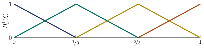
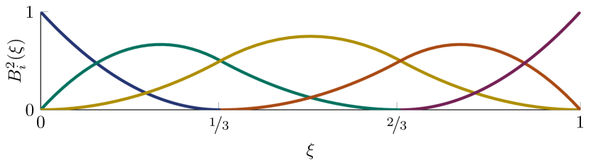
Figure 2: B-Spline basis functions of degree 1 and 2 on open, uniform knot vectors ($\Xi=\left[0,0,\nicefrac{{1}}{{3}},\nicefrac{{2}}{{3}},1,1\right]$ on top and $\Xi=\left[0,0,0,\nicefrac{{1}}{{3}},\nicefrac{{2}}{{3}},1,1,1\right]$ at the bottom).

Definitions (6) and (7) allow for an exact parametrization of conic sections such as circles and ellipses, which is of direct interest for the construction of the electric machine geometry, in particular of the air gap.

IGA utilizes the same Galerkin framework as FEM, but approximates the solution of a Partial Differential Equation (PDE) by a series expansion of NURBS (6). With respect to classical FEM spaces, the IGA spaces bring up several advantages, e.g., the inter-element smoothness of the basis functions which allows for a higher regularity of the solution across the elements. This property also leads to a significant reduction of the number of degrees of freedom required to achieve a certain accuracy [2, 6, 7]. The IGA system matrices are typically smaller than their FEM counterparts. This comes, however, at the expense of a larger bandwidth.

3 Stator-Rotor Coupling

Due to the topology and due to the presence of different materials, it is advantageous to construct the rotor and stator model parts of the PMSM independently. Each part is treated by a multipatch approach, i.e., by splitting the domain into several patches, each of them being the transformation of the unit square through a NURBS mapping. The degrees of freedom at the interfaces between the patches are glued together through static condensation in order to obtain global $C^{0}$ continuity [17]. It is worth mentioning that it would be possible to represent the entire computational domain as a single multipatch entity. Then, however, the total number of patches would increase significantly and the introduction of a relative angular displacement between stator and rotor would require a complicated mesh adaptation procedure or a complete reparametrization.

3.1 Domain decomposition

In this work, we propose to subdivide the full computational domain along a circular arc $\Gamma_{\text{ag}}=\overline{\Omega}_{\mathrm{rt}}\bigcap\overline{\Omega}_{\mathrm{st}}$ in the air gap, separating the two subdomains $\Omega_{\mathrm{rt}}$ and $\Omega_{\mathrm{st}}$ (Fig. 1). The rotor and stator patches are not required to be conforming on $\Gamma_{\text{ag}}$. The domain-decomposition approach reads

$$\left\{\begin{array}[]{rll}-\nabla\cdot\left(\nu\nabla A_{z,q}\right)&=J_{z}&\quad\text{in }\Omega_{q},\\ A_{z,q}|_{\Gamma_{\mathrm{d}}}&=0,&\\ A_{z,q}|_{\Gamma_{\mathrm{l}}}&=-A_{z,q}|_{\Gamma_{\mathrm{r}}},&\\ A_{z,\mathrm{rt}}|_{\Gamma_{\text{ag}}}&=A_{z,\mathrm{st}}|_{\Gamma_{\text{ag}}},&\\ \nu\nabla A_{z,\mathrm{rt}}|_{\Gamma_{\text{ag}}}\cdot\vec{n}_{\mathrm{st}}&=\nu\nabla A_{z,\mathrm{st}}|_{\Gamma_{\text{ag}}}\cdot\vec{n}_{\mathrm{st}},&\end{array}\right.$$ (8)

where $q\in\{\text{rt},\text{st}\}$ and $\vec{n}_{\mathrm{st}}$ is a unit vector perpendicular to the air gap interface directed from stator to rotor. The last two equations express the continuity of the magnetic vector potential and the continuity of the azimuthal component $H_{\theta}=\nu\nabla A_{z,\mathrm{rt}}|_{\Gamma_{\text{ag}}}\cdot\vec{n}_{\mathrm{st}}$ of the magnetic field strength. The two coupling approaches described below are distinct in the way they treat these interface conditions and set up the stator-rotor coupling.

3.2 Iterative substructuring

An iterative substructuring method invoking a Dirichlet-to-Neumann map for the first domain (here the rotor) followed by a Neumann-to-Dirichlet map for the second domain (here the stator) works as follows (see e.g. [18]). Let $\lambda^{0}$ be the initial solution for the magnetic vector potential at the air-gap interface $\Gamma_{\text{ag}}$ and let $k$ count the iteration steps. The domain-decomposion scheme (8) is carried out iteratively. First, a Poisson problem is solved for the rotor taking $\gamma^{k}$ as Dirichlet boundary condition at $\Gamma_{\text{ag}}$, i.e.,

$$\left\{\begin{array}[]{rll}-\nabla\cdot\left(\nu\nabla A_{z,\mathrm{rt}}^{k+1}\right)&=J_{z}&\text{in }\Omega_{\mathrm{rt}},\\ A_{z,\mathrm{rt}}^{k+1}|_{\Gamma_{\mathrm{d}}}&=0,&\\ A_{z,\mathrm{rt}}^{k+1}|_{\Gamma_{\mathrm{l}}}&=-A_{z,\mathrm{rt}}^{k+1}|_{\Gamma_{\mathrm{r}}},&\\ A_{z,\mathrm{rt}}^{k+1}|_{\Gamma_{\text{ag}}}&=\gamma^{k},&\end{array}\right.$$ (9)

from which the Neumann data $\nu\nabla A_{z,\mathrm{rt}}^{k+1}|_{\Gamma_{\text{ag}}}\cdot\vec{n}_{\mathrm{st}}$ is derived. Then, a Poisson problem is solved for the stator enforcing this Neumann data at $\Gamma_{\text{ag}}$, i.e.,

$$\left\{\begin{array}[]{rll}-\nabla\cdot\left(\nu\nabla A_{z,\mathrm{st}}^{k+1}\right)&=J_{z}&\text{in }\Omega_{\mathrm{st}},\\ A_{z,\mathrm{st}}^{k+1}|_{\Gamma_{\mathrm{d}}}&=0,&\\ A_{z,\mathrm{st}}^{k+1}|_{\Gamma_{\mathrm{l}}}&=-A_{z,\mathrm{st}}^{k+1}|_{\Gamma_{\mathrm{r}}},&\\ \nu\nabla A_{z,\mathrm{st}}^{k+1}|_{\Gamma_{\text{ag}}}\cdot\vec{n}_{\mathrm{st}}&=\nu\nabla A_{z,\mathrm{rt}}^{k+1}|_{\Gamma_{\text{ag}}}\cdot\vec{n}_{\mathrm{st}},&\end{array}\right.$$ (10)

from which updated Dirichlet data

$$\lambda^{k+1}=\alpha A_{z,\mathrm{st}}^{k+1}+(1-\alpha)\gamma^{k},$$ (11)

with $\alpha\in[0,1]$ a relaxation parameter, is obtained. A relaxation factor $\alpha<1$ is required to guarantee the convergence of the iterative substructuring approach [18]. As a stopping criterion for the method, the $L^{2}$ errors for the stator and rotor models between two successive iterations should be below a user-definied tolerance, both in the rotor and the stator, i.e.,

$$\varepsilon_{\text{rt}}=\left\|A_{z,\mathrm{rt}}^{k+1}-A_{z,\mathrm{rt}}^{k}\right\|_{L^{2}(\Omega_{\mathrm{rt}})}/\left\|A_{z,\mathrm{rt}}^{k+1}\right\|_{L^{2}(\Omega_{\mathrm{rt}})} <\texttt{tol},\quad\text{and}$$

$$\varepsilon_{\text{st}}=\left\|A_{z,\mathrm{st}}^{k+1}-A_{z,\mathrm{st}}^{k}\right\|_{L^{2}(\Omega_{\mathrm{st}})}/\left\|A_{z,\mathrm{st}}^{k+1}\right\|_{L^{2}(\Omega_{\mathrm{st}})} <\texttt{tol}.$$

The discretization of problems (9)-(10) is carried out in the IGA framework presented above. More details on this particular coupling approach can be found in [19]. In the following, a more sophisticated method is proposed.

3.3 Harmonic stator-rotor coupling

Let the polar coordinate system $(r,\theta)$ be connected to the stator and the polar coordinate system $(r,\theta^{\prime})$ be connected to the rotor. We denote by $\alpha$ the angular displacement between the two domains, i.e. $\theta^{\prime}=\theta-\alpha$. The interface conditions at $\Gamma_{\text{ag}}$ read

$$\left\{\begin{array}[]{rl}A_{z,\mathrm{st}}|_{\Gamma_{\text{ag}}}(\theta)&=A_{z,\mathrm{rt}}|_{\Gamma_{\text{ag}}}(\theta-\alpha),\\ H_{\theta,\mathrm{st}}(\theta)&=H_{\theta,\mathrm{rt}}(\theta-\alpha),\end{array}\right.$$ (12)

where $H_{\theta,\mathrm{st}}=\nu\nabla A_{z,\mathrm{st}}|_{\Gamma_{\text{ag}}}\cdot\vec{n}_{\mathrm{st}}$ and $H_{\theta,\mathrm{rt}}=\nu\nabla A_{z,\mathrm{rt}}|_{\Gamma_{\text{ag}}}\cdot\vec{n}_{\mathrm{st}}$.

The idea of harmonic stator-rotor coupling [20] is to express $H_{\theta,\mathrm{st}}(\theta)$ and $H_{\theta,\mathrm{rt}}(\theta^{\prime})$ in terms of a particular choice of basis functions. This approach can be interpreted in the context of Mortaring methods, with a particular choice of the space of Lagrange multipliers. A superposition of harmonic functions yields

$$H_{\theta,\mathrm{st}}(\theta) =\sum_{\ell\in L}\lambda_{\mathrm{st},\ell}e^{-\imath\ell\theta},$$ (13)

$$H_{\theta,\mathrm{rt}}(\theta^{\prime}) =\sum_{\ell\in L}\lambda_{\mathrm{rt},\ell}e^{-\imath\ell\theta^{\prime}},$$ (14)

where $\lambda_{\mathrm{st},\ell}$ and $\lambda_{\mathrm{rt},\ell}$ are the Fourier coefficients acting as degrees of freedom at the interface and $L$ is a given set of $N_{\Gamma}$ harmonics. The set $L$ only contains harmonic orders $\ell$ for which the corresponding harmonic functions $e^{-\imath\ell\theta}$ and $e^{-\imath\ell\theta^{\prime}}$ fulfill the same anti-periodic boundary conditions as applied to $\Gamma_{\mathrm{l}}$ and $\Gamma_{\mathrm{r}}$, e.g., $e^{-\imath\ell\theta}=e^{-\imath\ell(\theta+\tau_{\text{pole}})}$, where $\tau_{\text{pole}}$ is the angular extend of one pole (Fig. 1). The choice of harmonic trial functions enables us to construct a conforming discretization for $H_{\theta,\mathrm{st}}$ and $H_{\theta,\mathrm{rt}}$ at $\Gamma_{\text{ag}}$ and facilitates the application of the tangential continuity of the magnetic field strength in a strong way, leading to

$$\lambda_{\mathrm{st},\ell}=r_{\ell\ell}(\alpha)\lambda_{\mathrm{rt},\ell},$$ (15)

where the phase shifts $r_{\ell\ell}(\alpha)$ are gathered in the rotation matrix $\mathbf{R}(\alpha)$ such that (15) is in short $\bm{\lambda}_{\mathrm{st}}=\mathbf{R}(\alpha)\bm{\lambda}_{\mathrm{rt}}$.

The discretization of the Poisson equation in $\Omega_{\mathrm{st}}$ and $\Omega_{\mathrm{rt}}$ along the IGA framework leads to

$$\mathbf{K}_{\mathrm{st}}\mathbf{u}_{\mathrm{st}}+\mathbf{g}_{\mathrm{st}} =\mathbf{j}_{\mathrm{st}},$$ (16)

$$\mathbf{K}_{\mathrm{rt}}\mathbf{u}_{\mathrm{rt}}+\mathbf{g}_{\mathrm{rt}} =\mathbf{j}_{\mathrm{rt}},$$ (17)

where the additional term $\mathbf{g}_{\mathrm{st}}$ and $\mathbf{g}_{\mathrm{rt}}$ follow from integration by parts and are given by

$$g_{\mathrm{st},i} =-\int_{\Gamma_{\text{ag}}}H_{\theta,\mathrm{st}}(\theta)w_{i}(\theta)\;\text{d}\theta,$$ (18)

$$g_{\mathrm{rt},i} =\int_{\Gamma_{\text{ag}}}H_{\theta,\mathrm{rt}}(\theta^{\prime})w_{i}(\theta^{\prime})\;\text{d}\theta^{\prime}.$$ (19)

The introduction of the discretization of $H_{\theta,\mathrm{st}}$ and $H_{\theta,\mathrm{rt}}$ by harmonic functions leads to

$$\mathbf{g}_{\mathrm{st}} =\mathbf{G}_{\mathrm{st}}\mathbf{R}(\alpha)\bm{\lambda}_{\mathrm{rt}},$$ (20)

$$\mathbf{g}_{\mathrm{rt}} =\mathbf{G}_{\mathrm{rt}}\bm{\lambda}_{\mathrm{rt}},$$ (21)

where $\mathbf{G}_{\mathrm{st}}$ and $\mathbf{G}_{\mathrm{rt}}\in\mathbb{R}^{N_{\Gamma}\times N_{\text{DoF}}}$ are coupling matrices containing the integrals

$$g_{\mathrm{st},i\ell} =-\int_{\Gamma_{\text{ag}}}e^{-\imath\ell\theta}w_{i}(\theta)\;\text{d}\theta,$$ (22)

$$g_{\mathrm{rt},i\ell} =\int_{\Gamma_{\text{ag}}}e^{-\imath\ell\theta^{\prime}}w_{i}(\theta^{\prime})\;\text{d}\theta^{\prime},$$ (23)

combining IGA basis functions and harmonic functions (in the spirit of mortaring).

The continuity of the magnetic vector potential at the air-gap interface is imposed in a weak way, i.e., using the complex conjugate of the harmonic functions as test functions. This results in

$$-\mathbf{R}(\alpha)\mathbf{G}_{\mathrm{st}}^{H}\mathbf{u}_{\mathrm{st}}+\mathbf{G}_{\mathrm{rt}}^{H}\mathbf{u}_{\mathrm{rt}}=0,$$ (24)

where this expression turns out to include the hermitian transposes of the already calculated matrices.

Combining (16), (17) and (24) leads to the saddle-point problem

$$\left[\begin{array}[]{cc}\mathbf{K}&\mathbf{G}^{H}(\alpha)\\ \mathbf{G}(\alpha)&0\end{array}\right]\left[\begin{array}[]{c}\mathbf{U}\\ \bm{\lambda}_{\text{rt}}\end{array}\right]=\left[\begin{array}[]{c}\mathbf{J}\\ 0\end{array}\right],$$ (25)

with the blocks

$$\mathbf{K}=\begin{bmatrix}\mathbf{K}_{\mathrm{st}}&0\\ 0&\mathbf{K}_{\mathrm{rt}}\end{bmatrix},\;\mathbf{G}(\alpha)=\begin{bmatrix}-\mathbf{R}(\alpha)\mathbf{G}_{\mathrm{st}}&\mathbf{G}_{\mathrm{rt}}\end{bmatrix},\;\mathbf{U}=\begin{bmatrix}\mathbf{u}_{\mathrm{rt}}\\ \mathbf{u}_{\mathrm{st}}\end{bmatrix},\;\mathbf{J}=\begin{bmatrix}\mathbf{j}_{\mathrm{rt}}\\ \mathbf{j}_{\mathrm{st}}\end{bmatrix}.$$

The strategy proposed in this paper can be interpreted in the context of mortar methods [21], where the space of Lagrange multipliers is chosen as the space spanned by harmonic functions. We refer the interested reader to [22], for the application of mortaring to non-conforming FEM discretization of electrical machines, and to [23] for an overview of Isogeometric mortar methods.

3.4 Inf-sup condition

Problem (25) is a saddle-point problem and may give rise to instabilities when the number of harmonics in consideration $N_{\Gamma}$ is too big with respect to $N_{\mathrm{DoF}}$ [24]. The nature of these problems has been studied thoroughly in for example [25]. In order to guarantee stability the system should satisfy the inf-sup condition (see e.g. [26]). Here, the set $L$ only contains a few harmonic orders such that we are confident that the inf-sup condition is fulfilled in practice.

The stability of the saddle-point formulation (25) can be investigated numerically. To that purpose, we calculate the inf-sup constant $\beta$ using the method proposed in [27]. Given the stiffness matrix $\mathbf{K}$ and the coupling matrix $\mathbf{G}$, $\beta$ can be estimated by solving the eigenvalue problem

$$\mathbf{G}^{H}\mathbf{K}^{-1}\mathbf{G}\bm{\mathbf{x}}=\sigma^{2}\mathbf{M}\bm{\mathbf{x}},$$ (26)

with

$$m_{\ell k}=\int_{\Gamma_{\text{ag}}}e^{-jk\theta}e^{j\ell\theta}\;\text{d}\Gamma.$$ (27)

Given the sequence of eigenvalues $\sigma_{i}$ found by solving (26), the inf-sup constant can be obtained as

$$\beta=\min_{i}\sigma_{i}.$$ (28)

The stability of the saddle-point problem is guaranteed if $\beta$ is bounded away from zero.

3.5 Verification

To verify the proposed harmonic stator-rotor coupling in combination with IGA, we construct a simplified example for which a closed form solution exists. The geometry chosen for this test is a quarter of a ring with an inner radius of 1 m and an outer radius of 2 m (see Fig. 3). It is split in two annular domains to mimic the machine. Each domain is constructed as a multipatch geometry in such a way that the patch faces do not match at the connecting interface $\Gamma_{\text{ag}}$. To keep the analogy with the machine case, we will denote by $\Omega_{\mathrm{rt}}$ and $\Omega_{\mathrm{st}}$ the inner and outer domain respectively and $\overline{\Omega}=\overline{\Omega}_{\text{rt}}\bigcup\overline{\Omega}_{\text{st}}$. As a final simplification, we consider the Poisson’s equation with homogeneous Dirichlet boundary conditions

$$\left\{\begin{array}[]{rllrl}-\nabla\cdot\left(\nabla u\right)&=f&&\text{in }\Omega,\\ u&=0&&\text{on }\partial\Omega,\end{array}\right.$$ (29)

where

$$f=2x\left(22x^{2}y^{2}+21y^{4}-45y^{2}+x^{4}-5x^{2}+4\right).$$

This source term is chosen such that a closed form solution can be calculated [17].

The coupling presented in section 3.3 is tested for different choices of discretization degrees and number of coupling harmonics $N_{\Gamma}$. In Fig. 4 the $L^{2}$ error with respect to the exact solution is depicted for degree $p=1,2,3$ and $N_{\Gamma}=7$, with $L=\{-3,-2,\dots 3\}$. We recall that the $L^{2}$ error is defined as

$$\varepsilon_{L^{2}}:=\left\|u-u^{*}\right\|_{L^{2}}=\sqrt{\int_{\Omega}\left(u-u^{*}\right)^{2}\;\text{d}\Omega}.$$ (30)

As seen in Fig. 4, the coupling does not hinder the expected order of convergence, i.e. $O(h^{p+1})$.

Figure 3: Simplified geometry for verifying the harmonic stator-rotor coupling. The thick lines identify the two domains mimicking the rotor and the stator, while the thin lines show the non-conforming multipatch subdivisions. The color map shows the fabricated solution $u^{*}$.

Figure 4: Convergence of the computed solution to the exact solution for different choices of the discretization degree and for increasing mesh refinement. $N_{\Gamma}=7$ harmonics are used for the coupling ($\ell=-3,\dots,3$). The dashed lines show the expected order of convergence.

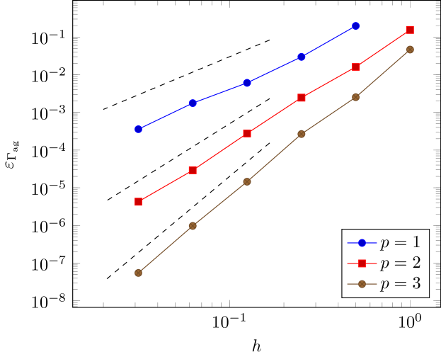
Figure 5: Convergence of the jump of the computed solution across the interface $\Gamma_{\text{ag}}$ in $L^{2}$ norm for different choices of the discretization degree and for increasing mesh refinement. $N_{\Gamma}=7$ harmonics are used for the coupling ($\ell=-3,\dots,3$). The dashed lines show the expected order of convergence.

The proposed coupling imposes weak continuity of $u$ across $\Gamma_{\text{ag}}$. As a further verification, we compute the jump of the computed solution across $\Gamma_{\text{ag}}$ and evaluate its $L^{2}$ norm, i.e.,

$$\varepsilon_{\Gamma_{\mathrm{ag}}}:=\left\|u_{\text{rt}|\Gamma_{\text{ag}}}-u_{\text{st}|\Gamma_{\text{ag}}}\right\|_{L^{2}}.$$ (31)

The results, depicted in Fig. 5, show the convergence of the method.

Finally, we consider the convergence of the Lagrange multipliers themselves. In particular, in Fig. 6, we show the convergence of the Neumann data to the exact solution, which can be evaluated as

$$\varepsilon_{\lambda,\mathrm{rt}}:=\left\|\nabla u^{*}\cdot\vec{n}_{\text{rt}}-\sum_{\ell\in L}\lambda_{\text{rt},\ell}e^{-i\ell\theta}\right\|_{L^{2}}.$$ (32)

The figure shows the good behavior of the Lagrange multipliers which converge with order $O(h^{2p})$.

Figure 6: Convergence of the Neumann data on $\Gamma_{\text{ag}}$ computed from the Lagrange multipliers to the exact solution in $L^{2}$ norm for different choices of the discretization degree and increasing mesh refinement. $N_{\Gamma}=7$ harmonics are used for the coupling ($\ell=-3,\dots,3$) The dashed lines show the order of convergence $O(h^{2p})$.

The inf-sup constant for an Isogeometric discretization of degree $2$ and increasing number of harmonics $N_{\Gamma}$ is presented in Fig. 7. It is apparent that when the spatial discretization is not fine enough (or, roughly said, the number of degrees of freedom is too low compared to the number of coupling harmonics), the saddle-point problem becomes unstable. For the considered applications, only a small number of harmonics with low orders is relevant. Expert knowledge can be used to choose the set $L$ appropriately.

Figure 7: Numerically evaluated inf-sup constant $\beta$ for a discretization of order 2 and different choices of the harmonics. When the spatial discretization is not fine enough, and when the number of harmonics increases, $\beta$ goes to zero.

4 Application: Permanent magnet synchronous machine

IGA with harmonic stator-rotor coupling is illustrated for a $6$-pole PMSM. Its design is described in [28]. The longitudinal length of the machine is 10 cm. The machine is constructed of laminated steel, which is modeled as iron with a vanishing conductivity. The PMSM is equipped with a $3$-phase, $6$-pole distributed double-layer winding with $12$ turns per half slot. The rotor contains $6$ buried NdFeB-magnets. The description of the geometric parameters and the material properties can be found in A.

FEMM [29] and the in-house code Niobe are used to solve (1) on $\Omega$ with classical FEM. The IGA framework is handled by the GeoPDEs package [17]. In post-processing, the spectrum of the electromotive force (EMF), i.e., the voltage induced in the open-circuit stator windings due to rotating the rotor at nominal speed, is calculated from the solution of (1). This is done under no-load conditions by applying the method proposed in [30]. One of the quality features of a PMSM is the total harmonic distortion (THD) defined by

$$\text{THD}=\frac{\sqrt{\sum_{p=2}^{\infty}|E_{p}|^{2}}}{|E_{1}|},$$ (33)

where $p$ represents the order and $E_{p}$ the Fourier coefficients of the EMF.

4.1 Comparison Between IGA and FEM

The rotor and stator domain are built using 12 and 78 patches respectively (see Fig. 1). On each subdomain, an IGA discretization is applied and the two coupling methods introduced in section 3 are used.

For the iterative substructuring approach, the implementation is straightforward and care must only be taken in the portion of $\Gamma_{\text{ag}}$ that require anti-symmetric boundary conditions (see problem 1). For harmonic stator-rotor coupling, as for the test case presented in section 3.5, the anti-periodic boundary conditions have an impact on the composition of the set $L$ of harmonic orders. To ensure the correct behavior at the boundaries, the harmonic orders cannot be chosen arbitrarily, i.e., they need to fulfil the anti-periodic boundary condition. The chosen set is $L_{\text{ap}}=\pm 3,\pm 9,\pm 15,\dots$, i.e., because of the $6$-pole symmetry, only multiple of $3$ need to be considered and because of the mirror symmetry within a single pole, all multiples of $6$ vanish. Furthermore, since we are looking for a real valued solution we always consider double sided spectrum, i.e. if $\ell$ is chosen, then $-\ell$ is also added to the set of coupling modes.

Table 1 reports the total computational effort of matrix assembly and solving for the two straightforward implementations. In the case of the iterative substructuring approach, the two matrices to be solved are obviously smaller than in the fully coupled system 25, but the iterative procedure leads to a slow overall procedure. In particular, the main bottleneck for the iterative substructuring approach is the evaluation of the Dirichlet and Neumann data on the common boundary $\Gamma_{\text{ag}}$ since, in the IGA context, the evaluation of the solution at given points in the physical domain is very expensive. This is due to the fact that this requires computing the inverse of the NURBS mapping in order to obtain the corresponding points in the reference domain. Given the non-linearity of the mapping, a Newton-Raphson scheme is typically used to perform this step, which considerably slows down the algorithm.

A second advantage of the proposed harmonic stator-rotor coupling is the straightforward handling of the relative rotation: for each relative angular displacement $\alpha$ only the rotation matrix has to be re-computed, which can happen at negligible cost. With iterative substructuring, instead, the right hand sides for both problems need to be re-assembled for each $\alpha$.

Table 1: Comparison of the computational efficiency between IGA with iterative substructuring and IGA with harmonic stator-rotor coupling. $t$ refers to the sum of assembly and solving time.

		DN (tol$=10^{-3}$)				Harmonic
Ref. Level	$p$	$N_{\text{DoF,rt}}$	$N_{\text{DoF,st}}$	$N_{\text{it}}$	Time (s)	$N_{\text{DoF}}$	Time (s)
1	1	32	193	9	67.021	241	3.335
2	1	137	746	9	123.462	908	6.610
4	1	563	2932	9	248.232	3538	13.675
8	1	2279	11624	9	528.551	13982	30.437
16	1	9167	46288	9	1200.739	55606	73.414
1	2	100	650	9	75.401	771	3.356
2	2	256	1515	10	161.381	1801	6.813
4	2	784	4325	10	330.292	5157	15.004
8	2	2704	14265	10	710.511	15053	33.953
16	2	10000	51425	9	1490.251	61581	85.595

We then consider IGA with harmonic stator-rotor coupling and compare it to a finite element model with a conforming discretisation in the air gap. The results for discretization degree $p=1,2$ are compared to a reference solution obtained using classical first order FEM on triangles [12] in Fig. 8. The simulation points shown in the plot correspond to the data given in Table 1.

Figure 8: Convergence of IGA with harmonic stator-rotor coupling ($\ell=\pm 3,\pm 9,\pm 15$) towards a first order FEM solution on a very fine mesh ($N_{\text{DoF}}=225667$).

In Fig. 9, parts of the spectra for the EMF calculated by FEM and by IGA are computed. The results for the EMF and the THD are listed in Table 2. The results for the EMF have a maximal relative difference below $3\%$. The relative difference for THD is higher, namely $6\%$, which might imply that the iterative substructuring introduces higher harmonics.

Figure 9: Spectrum with the first 32 modes of the EMF of the PMSM.

Table 2: Numerical results for the EMF and the THD.

	$E_{1}$	THD	$N_{\text{DoF}}$	Time (s)
FEM	29.8 V	5.72$\cdot$10-2 $\%$	225667	103.45
IGA-HC	30.4 V	5.87$\cdot$10-2 $\%$	5157	15.00
IGA-DN	30.6 V	6.06$\cdot$10-2 $\%$	5109	330.29

5 Conclusion

In this work IGA has been applied to model a PMSM. Since it is possible to parametrize circular arcs exactly, geometric approximations, from which the classical FEMs suffer, are avoided. A multipatch approach is used to model the rotor and the stator separately. The coupling between the two parts has been carried out by iterative substructuring or by using harmonic basis functions. To test the latter so-called harmonic stator-rotor coupling, a test case has been constructed for which the convergence of the spatial discretization has been shown. The harmonic stator-rotor coupling leads to a saddle-point problem for which our setting attains stability. As illustrated by the example, IGA with harmonic stator-rotor coupling is a new and promising alternative to standard finite element procedures for electric machine simulation.

Appendix A Machine parameters

The parameters of the machine are listed in Tab. 1 and in Tab. 2. The geometrical parameters are depicted in Fig. 1.

Figure 1: Geometry of the PMSM

Table 1: Parameters describing the geometry of the machine

Rotor
Inner radius rotor	$R_{\mathrm{rt,i}}$	16 mm
Outer radius rotor	$R_{\mathrm{rt,o}}$	44 mm
Magnet width	$d_{1}$	19 mm
Magnet height	$d_{2}$	7 mm
Depth of the magnet in rotor	$d_{3}$	7 mm
	$\delta_{1}$	8.5 °
	$\delta_{2}$	42 °
Stator
Inner radius stator	$R_{\mathrm{st,i}}$	45 mm
Outer radius stator	$R_{\mathrm{st,o}}$	67.5 mm
Number of turns	$N_{w}$	12
	$\delta_{3}$	7 °
	$\delta_{4}$	5.7 °
	$\delta_{5}$	4 °
	$l_{1}$	0.6 mm
	$l_{2}$	5.4 mm
	$l_{3}$	5 mm
	$l_{4}$	8.2 mm
Skew angle	$\varphi$	0.52 °
Air gap
Radius of $\Gamma_{\text{ag}}$	$R_{\mathrm{ag}}$	44.7 mm

Table 2: Parameters describing the material properties

Material properties
Conductivity of iron	$\sigma_{\mathrm{Fe}}$	0 S/m
Conductivity of copper	$\sigma_{\mathrm{Cu}}$	4.3$\cdot 10^{7}$ S/m
Conductivity of PM	$\sigma_{\mathrm{PM}}$	6667 S/m
Relative permeability of iron	$\mu_{\mathrm{r,Fe}}$	500
Relative permeability of copper	$\mu_{\mathrm{r,Cu}}$	1
Relative permeability of PM	$\mu_{\mathrm{r,PM}}$	1.5
Remanent magnetic field of PM	$B_{\mathrm{r}}$	0.94 T

References

References

- [1] T.J.R. Hughes, J.A. Cottrell and Y. Bazilevs, Isogeometric analysis: CAD, finite elements, NURBS, exact geometry and mesh refinement, Comput. Meth. Appl. Mech. Eng., 194 (2005) 4135–4195.
- [2] J.A. Cottrell, T.J.R. Hughes and Y. Bazilevs, Isogeometric Analysis: Toward Integration of CAD and FEA, John Wiley & Sons, Ltd, 2009.
- [3] I. Temizer, P. Wriggers and T.J.R. Hughes, Contact treatment in isogeometric analysis with NURBS, Comput. Meth. Appl. Mech. Eng., 200(9) (2011) 1100–1112.
- [4] H. Gomez, T.J.R. Hughes, X. Nogueira and V.M. Calo, Isogeometric analysis of the isothermal Navier–Stokes–Korteweg equations, Comput. Meth. Appl. Mech. Eng. 199(25) (2010) 1828 – 1840.
- [5] V.P. Nguyen, C. Anitescu, S.P.A. Bordas and T. Rabczuk, Isogeometric analysis: An overview and computer implementation aspects, Math. Comput. Simulation 117 (2015) 89–116.
- [6] T.J.R. Hughes, J.A. Evans, A. Reali, “Finite element and NURBS approximations of eigenvalue, boundary-value, and initial-value problems”, Computer Methods in Applied Mechanics and Engineering, 272, 290-320, 2014.
- [7] J. Corno, C. de Falco, H. De Gersem and S. Schöps, “Isogeometric simulation of Lorentz detuning in superconducting accelerator cavities” Computer Physics Communications, 201, 1-7, 2016.
- [8] D. Howe and Z.Q. Zhu, The influence of finite element discretisation on the prediction of cogging torque in permanent magnet excited motors, IEEE Trans. Magn. 28(2) (1992) 1080–1083.
- [9] A. Pels, Z. Bontinck, J. Corno, H. De Gersem and S. Schöps, Optimization of a Stern-Gerlach Magnet by Magnetic Field-Circuit Coupling and Isogeometric Analysis, IEEE Trans. Magn. 51(12) (2015) 1–7.
- [10] E. Vassent, G. Meunier and J.C. Sabonnadière, Simulation of induction machine operation using complex magnetodynamic finite elements, IEEE Trans. Magn. 25(4) (1989) 3064–3066.
- [11] N. Sadowski, B. Carly, Y. Lefevre, M. Lajoie-Mazenc, S. Astier, Finite element simulation of electrical motors fed by current inverters, IEEE Trans. Magn. 29(2) (1993) 1683–1688.
- [12] S.J. Salon, Finite element analysis of electrical machines, Boston USA: Kluwer academic publishers, 1995.
- [13] N. Bianchi, Electrical machine analysis using finite elements, CRC press, 2005.
- [14] P. Monk, Finite Element Methods for Maxwell’s Equations, Oxford: Oxford University Press, 2003
- [15] A. Buffa, G. Sangalli, and R. Vázquez, Isogeometric analysis in electromagnetics: B-splines approximation, Computer Methods in Applied Mechanics and Engineering, 199(17), 1143-1152, 2010.
- [16] L. Piegl and W. Tiller. “The NURBS book”, Monographs in Visual Communication, 1997.
- [17] R. Vázquez, A new design for the implementation of isogeometric analysis in Octave and Matlab: GeoPDEs 3.0, Computers & Mathematics with Applications 72(3) (2016) 523–554.
- [18] A. Quarteroni and A. Valli, “Domain decomposition methods for partial differential equations”, Oxford University Press, 1999.
- [19] P. Bhat, Z. Bontinck, J. Corno, H. De Gersem, S. Schöps, “Modelling of a Permanent Magnet Synchronous Machine Using Isogeometric Analysis”, to appear In: 18th International Symposium on Electromagnetic Fields in Mechatronics, Electrical and Electronic Engineering, Łódź, Poland, 2017.
- [20] H. De Gersem and T. Weiland, Harmonic weighting functions at the sliding interface of a finite-element machine model incorporating angular displacement, IEEE Trans. Magn. 40(2) (2004) 545–548.
- [21] F.B. Belgacem, The mortar finite element method with Lagrange multipliers, Numerische Mathematik, 84(2), 173-197, 1999.
- [22] A. Buffa, Y. Maday, and F. Rapetti, A Slideing Mesh-Mortar Method for a two Dimensional Currents Model of Electric Engines, ESAIM: Mathematical Modelling and Numerical Analysis, 35(2), 191-228, 2001.
- [23] E. Brivadis, A. Buffa, B. Wohlmuth, and L. Wunderlich, Isogeometric mortar methods, Computer Methods in Applied Mechanics and Engineering, 284, 292-319, 2015.
- [24] F. Brezzi and M. Fortin, Mixed and hybrid finite element methods, Springer Science & Business Media 15 (2012).
- [25] F. Brezzi, On the existence, uniqueness and approximation of saddle-point problems arising from Lagrangian multipliers, Rev. française Automat., informat., recherche opérationnelle Sér. Rouge 8(R2) (1974) 129–151.
- [26] K.-J. Bathe, The inf–sup condition and its evaluation for mixed finite element methods, Computers & structures 79(2) (2001) 243–252.
- [27] D. Chapelle and K.-J. Bathe, The inf-sup test, Computers & structures 47(4-5) (1993) 537–545.
- [28] S. Henneberger, U. Pahner, K. Hameyer and R. Belmans, Computation of a highly saturated permanent magnet synchronous motor for a hybrid electric vehicle, IEEE Trans. Magn., 33(5) (1997) 4086–4088.
- [29] D. Meeker, Finite Element Method Magnetics User’s Manual, http://www.femm.info/, Version 4.2 (09Nov2010 Build), 2010.
- [30] M.A. Rahman and P. Zhou, Determination of saturated parameters of PM motors using loading magnetic fields, IEEE Trans. Magn., 27(5) (1991) 3947–3950.