An Approximate Solver for Multi-medium Riemann Problem with Mie-Grüneisen Equations of State

Abstract

We propose an approximate solver for multi-medium Riemann problems with materials described by a family of general Mie-Grüneisen equations of state, which are widely used in practical applications. The solver provides the interface pressure and normal velocity by an iterative method. The well-posedness and convergence of the solver is verified with mild assumptions on the equations of state. To validate the solver, it is employed in computing the numerical flux on phase interfaces of a numerical scheme on Eulerian grids that was developed recently for compressible multi-medium flows. Numerical examples are presented for Riemann problems, air blast and underwater explosion applications.

1 Introduction

Numerical simulations of compressible multi-medium flow are of great interest in practical applications, such as mechanical engineering, chemical industry, and so on. Many conservative Eulerian algorithms perform very well in single-medium compressible flows. However, when such an algorithm is employed to compute multi-medium flows, numerical inaccuracies may occur at the material interfaces [1, 2, 3], due to the great discrepancy of densities and equations of state across the interface. The simulation of compressible multi-medium flow in an Eulerian framework requires special attention in describing the interface connecting distinct fluids, especially for the problems that involve highly nonlinear equations of state. Several techniques have been taken to treat the multi-medium flow interactions. See [3, 4, 5, 6, 7, 8, 9] for instance.

A typical procedure of multi-medium compressible flows in Eulerian grids mainly consists of two steps, the interface capture and the interaction between different fluids. There are mainly two different approaches in literatures, the diffuse interface method (DIM) and the sharp interface method (SIM). The former [1, 4, 8, 10, 11, 12] assumes the interface as a diffuse zone, and smears out the interface over a certain number of grid cells to avoid pressure oscillations. Diffuse interfaces correspond to artificial mixtures created by numerical diffusion, and the key issue is to fulfill interface conditions within this artificial mixture. The latter assumes the interface to be a sharp contact discontinuity, and different fluids are immiscible. Several approaches such as the volume of fluid (VOF) method [13, 14], level set method [15, 16], moment of fluid (MOF) method [17, 18, 19] and front-tracking method [20, 21] are used extensively to capture the interface. A key element for both diffuse and sharp interface methods, is to determine the interface states. The accurate prediction of the interface states can be used to stabilize the numerical diffusion in diffuse interface methods, and to compute the numerical flux and interface motion in sharp interface methods. One common approach is to solve a multi-medium Riemann problem which contains the fundamentally physical and mathematical properties of the governing equations. Indeed, the Riemann problem plays a key role in understanding the wave structures, since a general fluid flow may be interpreted as a nonlinear superpositions of the Riemann solutions.

The solution of a multi-medium Riemann problem depends not only on the initial states at each side of the interface, but also on the forms of equations of state. For some simple equations of state, such as ideal gas, covolume gas or stiffened gas, the solution of the Riemann problem can be achieved to any desired accuracy with an exact solver. While the Riemann problems for the above equations of state have been fully investigated in [22, 23, 24, 25] for instance, there exist some difficulties in the cases of general nonlinear equations of state due to their high nonlinearity. A variety of methods to solve the corresponding Riemann problems have then been proposed. For example, Larini et al. [26] developed an exact Riemann solver and applied their methods to a fifth-order virial equation of state (EOS), which is particularly suited to the gaseous detonation products of high explosive compounds. Shyue [7] developed a Roe’s approximate Riemann solver for the Mie-Grüneisen EOS with variable Grüneisen coefficient. Quartapelle et al. [27] proposed an exact Riemann solver by applying the Newton-Raphson iteration to the system of two nonlinear equations imposing the equality of pressure and of velocity, assuming as unknowns the two values of the specific volume at each side of the interface, and implemented it for the van der Waals gas. Arienti et al. [6] applied a Roe-Glaster solver to compute the equations combining the Euler equations involving chemical reaction with the Mie-Grüneisen EOS. More recently, Rallu [28] and Farhat et al. [29] utilized a sparse grid technique to tabulate the solutions of exact multi-medium Riemann problems. Lee et al. [30] developed an exact Riemann solver for the Mie-Grüneisen EOS with constant Grüneisen coefficient, where the integral terms are evaluated using an iterative Romberg algorithm. Banks [31] and Kamm [32] developed a Riemann solver for the convex Mie-Grüneisen EOS by solving a nonlinear equation for the density increment involved in the numerical integration of rarefaction curves, and chose the JWL (Jones-Wilkins-Lee) EOS as a representative case.

In this paper, we propose an approximate multi-medium Riemann solver for a family of general Mie-Grüneisen equations of state in an iterative manner, which provides a strategy to reproduce the physics of interaction between two mediums across the interface. Several mild conditions on the coefficients of Mie-Grüneisen EOS are assumed to ensure the convexity of equations of state and the well-posedness of our Riemann solver. The algebraic equation of the Riemann problem is solved by an inexact Newton method [33], where the function and its derivative are evaluated approximately depending on the wave configuration. And the convergence of our Riemann solver is analyzed. To validate the proposed solver, we employed it in the computation of two-medium compressible flows with Mie-Grüneisen EOS, as an extension of the numerical scheme that was developed recently for two-medium compressible flows with ideal gases [34].

The rest of this paper is arranged as follows. In Section 2, a solution strategy for the multi-medium Riemann problem with arbitrary Mie-Grüneisen equations of state is presented. In Section 3, the procedures of our approximate Riemann solver are outlined, and the well-posedness and convergence are analyzed. In Section 4, the application of our Riemann solver in two-medium compressible flow calculations [34] is briefly introduced. In Section 5, several classical Riemann problems and applications for air blast and underwater explosions are carried out to validate the accuracy and robustness of our solver. Finally, a short conclusion is drawn in Section 6.

2 Multi-medium Riemann Problem

Let us consider the following one-dimensional multi-medium Riemann problem of the compressible Euler equations

$$\dfrac{\partial}{\partial\tau}\begin{bmatrix}\rho\\ \rho u\\ E\end{bmatrix}+\dfrac{\partial}{\partial\xi}\begin{bmatrix}\rho u\\ \rho u^{2}+p\\ (E+p)u\end{bmatrix}=\bm{0},\quad E=\rho e+\dfrac{1}{2}\rho u^{2}.$$ (1a)

Here $$\tau \xi \rho u p E e$$ is time and is spatial coordinate, and , , , and are the density, velocity, pressure, total energy and specific internal energy, respectively. The system has initial values

$$[\rho,u,p]^{\top}(\xi,\tau=0)=\begin{cases}[\rho_{l},u_{l},p_{l}]^{\top},&\xi<0,\\ [\rho_{r},u_{r},p_{r}]^{\top},&\xi>0.\end{cases}$$ (1b)

Here the equations of state for both mediums under our consideration can be classified into the family known as the Mie-Grüneisen EOS. The Mie-Grüneisen EOS can be used to describe a lot of real materials, for example, the gas, water and gaseous products of high explosives [6, 3, 32], which is particularly useful in those practical applications we are studying now. The general form of the Mie-Grüneisen EOS is given by

$$p(\rho,e)=\varGamma(\rho)\rho e+h(\rho),$$ (2)

where $\varGamma(\rho)$ is the Grüneisen coefficient, and $h(\rho)$ is a reference state associated with the cold contribution resulting from the interactions of atoms at rest [35]. Thus the EOS of the multi-medium Riemann problem (1b) is given by

$$p(\rho,e)=\begin{cases}\varGamma_{l}(\rho)\rho e+h_{l}(\rho),\\ \varGamma_{r}(\rho)\rho e+h_{r}(\rho),\end{cases}$$

for the medium on the left and the right sides, respectively. For the ease of our analysis, we impose on $\varGamma(\rho)$ and $h(\rho)$ the following assumptions:

(C1) $\varGamma^{\prime}(\rho)\leq 0,~{}(\rho\varGamma(\rho))^{\prime}\geq 0,~{}(\rho\varGamma(\rho))^{\prime\prime}\geq 0$;

(C2) $\lim\limits_{\rho\rightarrow+\infty}\varGamma(\rho)=\varGamma_{\infty}>0,~{}\varGamma(\rho)\leq\varGamma_{\infty}+2$;

(C3) $h^{\prime}(\rho)\geq 0,~{}h^{\prime\prime}(\rho)\geq 0$.

Remark 1.

An immediate consequence is that the Grüneisen coefficient $\varGamma(\rho)$ must be nonnegative since $\varGamma(\rho)\geq-\varGamma^{\prime}(\rho)\rho\geq 0$ by the condition (C1).

A lot of equations of state of our interests fulfill these assumptions. Particularly, we collect some equations of state in Appendix A which are used in our numerical tests as examples. These examples include ideal gas EOS, stiffened gas EOS, polynomial EOS, JWL EOS, and Cochran-Chan EOS. The coefficients $\varGamma(\rho)$, $h(\rho)$ and their derivatives for these equations of state are all provided therein.

The Riemann problem for general convex equations of state have been fully analyzed, for example, in [36, 37]. Here the problem is more specific, thus we can present the structure of the solution in a straightforward way. The property of EOS is essential on the wave structures in the solution of Riemann problems. It is pointed out that the wave structures are composed solely of elementary waves [37] if the fundamental derivative [38]

$$\mathscr{G}=\dfrac{1}{c}\cdot\left.\dfrac{\partial\rho c}{\partial\rho}\right|_{s}=1+\dfrac{\rho}{2c^{2}}\cdot\left.\dfrac{\partial c^{2}}{\partial\rho}\right|_{s},$$

keeps positive , where $s$ is the specific entropy and $c$ is the speed of sound. For the Mie-Grüneisen EOS (2), the speed of sound can be expressed as

$$c(p,\rho)=\sqrt{\left.\dfrac{\partial p}{\partial\rho}\right|_{e}+\dfrac{p}{\rho^{2}}\left.\dfrac{\partial p}{\partial e}\right|_{\rho}}=\sqrt{\left(\dfrac{1}{\rho}+\dfrac{\varGamma_{k}^{\prime}(\rho)}{\varGamma_{k}(\rho)}\right)(p-h_{k}(\rho))+\dfrac{p}{\rho}\varGamma_{k}(\rho)+h_{k}^{\prime}(\rho)},$$

and a tedious calculus gives us that the fundamental derivative is

$$\begin{split}\mathscr{G}=&\dfrac{1}{c^{2}}\left(\dfrac{1}{2}\left(\rho(\rho\varGamma_{k}(\rho))^{\prime\prime}+{(\rho\varGamma_{k}(\rho))^{\prime}}(2+\varGamma_{k}(\rho))\right)e+\dfrac{1}{2}\rho h_{k}^{\prime\prime}(\rho)\right.\\ &\left.+\dfrac{p}{2\rho}(\varGamma_{k}^{2}(\rho)+2(\rho\varGamma_{k}(\rho))^{\prime})+\dfrac{1}{2}(2+\varGamma_{k}(\rho))h_{k}^{\prime}(\rho)\right).\end{split}$$ (3)

We conclude that

Lemma 1.

The solution of the multi-medium Riemann problem (1b) consists of only elementary waves if the conditions (C1), (C2) and (C3) are fulfilled.

Proof.

With the conditions (C1), (C2) and (C3), a direct check on the terms in (3) gives us that

$$\mathscr{G}>0,$$

then the result in [37] is applied to give us the conclusion. ∎

Precisely, the solution of (1b) consists of four constant regions connected by a linearly degenerate wave and two genuinely nonlinear waves (either shock wave or rarefaction wave, depending on the initial states), as is shown schematically in Fig. 1. The linearly degenerate wave is actually the phase interface.

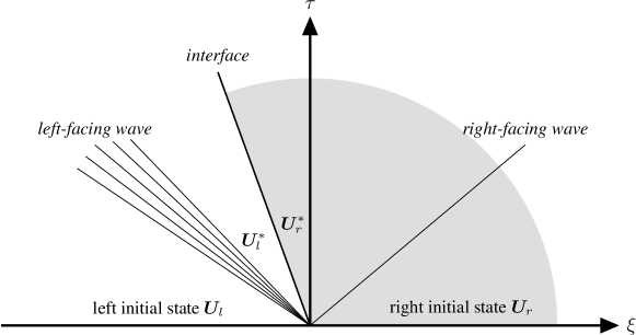
Figure 1: Typical wave structure of the Riemann problem in $\xi-\tau$ space.

Following the convention on notations, we denote the pressure and the velocity by $p^{*}$ and $u^{*}$ in the star region, respectively, which have the same value crossing over the phase interface. This allows us to derive a single nonlinear algebraic equation for $p^{*}$. Then we will solve this algebraic equation by an iterative method. At the beginning of each step of the iterative method, a provisional value of $p^{*}$ determines the wave structures from four possible configurations. The wave structures then prescribe the specific formation of the algebraic equation. Based on the residual of the algebraic equation, the value of $p^{*}$ is updated, which closes a single loop of the iterative method.

Below let us give the details of the plan above. Firstly we need to study the relations of the solution across a nonlinear wave, saying a shock wave or a rarefaction wave. For convenience, we use the subscript $k=l$ or $r$ standing for either the left initial state $l$ or the right initial state $r$ hereafter.

• Solution through a shock wave

  If $p^{*}>p_{k}$, the corresponding nonlinear wave is a shock wave, and the star region state $\bm{U}_{k}^{*}$ is connected to the adjacent initial state $\bm{U}_{k}$ through a Hugoniot locus. The Rankine-Hugoniot jump conditions [25] yield

  $$\mp(u^{*}-u_{k})=\left((p^{*}-p_{k})\left(\dfrac{1}{\rho_{k}}-\dfrac{1}{\rho^{*}_{k}}\right)\right)^{1/2},$$ (4)

  and

  $$e(p^{*},\rho^{*}_{k})-e(p_{k},\rho_{k})+\dfrac{1}{2}(p^{*}+p_{k})\left(\dfrac{1}{\rho^{*}_{k}}-\dfrac{1}{\rho_{k}}\right)=0,$$ (5)

  where

  $$e(p,\rho)=\dfrac{p-h_{k}(\rho)}{\varGamma_{k}(\rho)\rho}.$$

  Multiplying both sides of the equality (5) by $\rho_{k}\rho_{k}^{*}\varGamma_{k}(\rho_{k})\varGamma_{k}(\rho_{k}^{*})$ gives rise to

  $$\begin{split}&\varGamma_{k}(\rho_{k})\rho_{k}(p^{*}-h_{k}(\rho_{k}^{*}))-\varGamma_{k}(\rho_{k}^{*})\rho_{k}^{*}(p_{k}-h_{k}(\rho_{k}))\\ &-\dfrac{1}{2}\varGamma_{k}(\rho_{k}^{*})\varGamma_{k}(\rho_{k})(p^{*}+p_{k})(\rho_{k}^{*}-\rho_{k})=0.\end{split}$$

  For convenience we introduce the Hugoniot function as follows

  $$\begin{split}\varPhi_{k}(p,\rho)&:=\varGamma_{k}(\rho_{k})\rho_{k}(p-h_{k}(\rho))-\varGamma_{k}(\rho)\rho(p_{k}-h_{k}(\rho_{k}))\\ &-\dfrac{1}{2}\varGamma_{k}(\rho_{k})(p+p_{k})\varGamma_{k}(\rho)(\rho-\rho_{k}),\end{split}$$ (6)

  then the relation (5) boils down to the algebraic equation $\varPhi_{k}(p^{*},\rho_{k}^{*})=0$. The derivative of $\varPhi_{k}$ with respect to the density is found to be

  $$\begin{split}\dfrac{\partial\varPhi_{k}}{\partial\rho}(p,\rho)&=-\varGamma_{k}(\rho_{k})\rho_{k}\left(h_{k}^{\prime}(\rho)-\dfrac{p+p_{k}}{2}\varGamma_{k}^{\prime}(\rho)\right)\\ &-\varGamma_{k}(\rho_{k})(\varGamma_{k}(\rho)+\rho\varGamma_{k}^{\prime}(\rho))\left(\rho_{k}e_{k}+\dfrac{p+p_{k}}{2}\right).\end{split}$$ (7)

  As a result, the slope of the Hugoniot locus can be found by the method of implicit differentiation, namely,

  $$\chi(p,\rho):=\left.\dfrac{\partial p}{\partial\rho}\right|_{\varPhi_{k}}=-\dfrac{2\partial\varPhi_{k}(p,\rho)/\partial\rho}{\varGamma_{k}(\rho_{k})(2\rho_{k}-{\varGamma_{k}(\rho)}(\rho-\rho_{k}))}.$$

  Before we discuss the properties of the Hugoniot function $\varPhi_{k}(p,\rho)$, let us introduce the compressive limit of the density $\rho_{\max}$ such that $\chi(p,\rho_{\max})=\infty$. By definition $\rho_{\max}$ solves the algebraic equation $2\rho_{k}-\varGamma_{k}(\rho)(\rho-\rho_{k})=0$. This quantity is uniquely defined since the function

  $$W(\rho):=\left(\dfrac{\rho}{\rho_{k}}-1\right)\varGamma_{k}(\rho)-2,$$

  is monotonically increasing in the interval $(\rho_{k},+\infty)$ by the condition (C1), and

  $$W(\rho_{k})=-2,\quad\lim_{\rho\rightarrow+\infty}W(\rho)\geq\lim_{\rho\rightarrow+\infty}\left(\dfrac{\rho}{\rho_{k}}-1\right)\varGamma_{\infty}-2=+\infty.$$

  We have the following results on the function $\varPhi_{k}(p,\rho)$

  Lemma 2.

  Assume that the functions $\varGamma_{k}(\rho)$ and $h_{k}(\rho)$ satisfy the conditions (C1), (C2) and (C3). Then $\varPhi_{k}(p,\rho)$ defined in (6) satisfies the following properties:

  • $\varPhi_{k}(p,\rho_{k})>0$;

  • $\varPhi_{k}(p,\rho_{\max})<0$;

  • ${\partial\varPhi_{k}}(p,\rho)/{\partial\rho}<0$;

  • ${\partial^{2}\varPhi_{k}}(p,\rho)/{\partial\rho^{2}}<0$ if $\varGamma^{\prime\prime}_{k}(\rho)=0$.

  Proof.

  (1). By definition (6) we have

  $$\begin{split}\varPhi_{k}(p,\rho_{k})&=\varGamma_{k}(\rho_{k})\rho_{k}(p-h_{k}(\rho_{k}))-\varGamma_{k}(\rho_{k})\rho_{k}(p_{k}-h_{k}(\rho_{k}))\\ &=\varGamma_{k}(\rho_{k})\rho_{k}(p-p_{k})>0.\end{split}$$

  (2). Since the compressive limit of the density $\rho_{\max}$ satisfies the relation $(\rho_{\max}-\rho_{k})\varGamma_{k}(\rho_{\max})=2\rho_{k}$, we have

  $$\begin{split}&\varPhi_{k}(p,\rho_{\max})\\ =&\varGamma_{k}(\rho_{k})\rho_{k}(p-h_{k}(\rho_{\max}))-\varGamma_{k}(\rho_{\max})\rho_{\max}(p_{k}-h_{k}(\rho_{k}))\\ -&\dfrac{1}{2}\varGamma_{k}(\rho_{\max})(\rho_{\max}-\rho_{k})\varGamma_{k}(\rho_{k})(p+p_{k})\\ =&-\varGamma_{k}(\rho_{k})\rho_{k}(p_{k}+h_{k}(\rho_{\max}))-(\varGamma_{k}(\rho_{\max})+2)\rho_{k}(p_{k}-h_{k}(\rho_{k})).\end{split}$$ (8)

  Obviously $\varPhi_{k}(p,\rho_{\max})<0$ if $h_{k}(\rho_{\max})\geq 0$. On the other hand, suppose that $h_{k}(\rho_{\max})<0$. Rewriting (8) as

  $$\begin{split}\varPhi_{k}(p,\rho_{\max})&=-(\varGamma_{k}(\rho_{k})+\varGamma_{k}(\rho_{\max})+2)\rho_{k}p_{k}\\ &-\rho_{k}(\varGamma_{k}(\rho_{k})h_{k}(\rho_{\max})-(\varGamma_{k}(\rho_{\max})+2)h_{k}(\rho_{k})),\end{split}$$

  and using the inequality resulting from the conditions (C2) and (C3)

  $$\varGamma_{k}(\rho_{k})h_{k}(\rho_{\max})\geq\varGamma_{k}(\rho_{k})h_{k}(\rho_{k})\geq(\varGamma_{\infty}+2)h_{k}(\rho_{k})\geq(\varGamma_{k}(\rho_{\max})+2)h_{k}(\rho_{k}),$$

  we conclude that $\varPhi_{k}(p,\rho_{\max})<0$.

  (3). This is an obvious result from the expression (7).

  (4). The second derivative of $\varPhi_{k}(p,\rho)$ with respect to the density is

  $$\begin{split}\dfrac{\partial^{2}\varPhi_{k}}{\partial\rho^{2}}(p,\rho)&=-\varGamma_{k}(\rho_{k})\rho_{k}\left(h_{k}^{\prime\prime}(\rho)-\dfrac{p+p_{k}}{2}\varGamma_{k}^{\prime\prime}(\rho)\right)\\ &-\varGamma_{k}(\rho_{k})(2\varGamma_{k}^{\prime}(\rho)+\rho\varGamma_{k}^{\prime\prime}(\rho))\left(\rho_{k}e_{k}+\dfrac{p+p_{k}}{2}\right),\end{split}$$

  which is negative if $\varGamma^{\prime\prime}_{k}(\rho)=0$. This completes the proof of the whole theorem. ∎

  Instantly by Lemma 2, the density $\rho$ can be uniquely determined from the equation $\varPhi_{k}(p,\rho)=0$ on the interval $(\rho_{k},\rho_{\max})$ for any fixed $p$. Also the Hugoniot curve is monotonic due to $\chi>0$. Since the equation (5) uniquely defines the interface density $\rho_{k}^{*}$ for a given value of $p^{*}$, the right hand side of (4) can be regarded as a function of the interface pressure $p^{*}$ alone, formally written as

  $$f_{k}(p^{*})=\left((p^{*}-p_{k})\left(\dfrac{1}{\rho_{k}}-\dfrac{1}{\rho^{*}_{k}}\right)\right)^{1/2},\quad p^{*}>p_{k}.$$

• Solution through a rarefaction wave

  If, on the other hand, $p^{*}\leq p_{k}$, then the corresponding nonlinear wave is a rarefaction wave, and the interface state $\bm{U}_{k}^{*}$ is connected to the adjacent initial state $\bm{U}_{k}$ through a rarefaction curve. Since the Riemann invariant

  $$u\pm\int\dfrac{1}{\rho c}\mathrm{d}p,$$

  is constant along the right-facing (left-facing) rarefaction curve, we have

  $$\mp(u^{*}-u_{k})=\int_{p_{k}}^{p^{*}}\dfrac{1}{\rho c}\mathrm{d}p,$$ (9)

  where the density $\rho$ is expressed in terms of $p$ by solving the isentropic relation

  $$\dfrac{\partial p}{\partial\rho}=c^{2}(p,\rho).$$ (10)

  Similarly, the right hand side of (9) can be expressed as a function of $p^{*}$ alone. Formally we define

  $$f_{k}(p^{*})=\int^{p^{*}}_{p_{k}}\dfrac{1}{\rho c}\mathrm{d}p,\quad p^{*}\leq p_{k}.$$

Collecting both cases above, we have that

$$u^{*}-u_{l}=-f_{l}(p^{*})\quad\text{ and }\quad u^{*}-u_{r}=f_{r}(p^{*}).$$

Therefore, the interface pressure $p^{*}$ is the zero of the following pressure function

$$f(p):=f_{l}(p)+f_{r}(p)+u_{r}-u_{l}.$$

And the interface velocity $u^{*}$ can be determined by

$$u^{*}=\dfrac{1}{2}(u_{l}+u_{r}+f_{r}(p^{*})-f_{l}(p^{*})).$$

Recall that the formula of the function $f_{k}(p)$ is given by

$$f_{k}(p)=\begin{cases}\displaystyle\int^{p}_{p_{k}}\dfrac{1}{\rho c}\mathrm{d}p,&p\leq p_{k},\\ \left((p-p_{k})\left(\dfrac{1}{\rho_{k}}-\dfrac{1}{\rho}\right)\right)^{1/2},&p>p_{k},\end{cases}$$

where $\rho$ is determined through either the Hugoniot relation (5) or the isentropic relation (10) for a given $p$. We claim on $f_{k}(p)$ that

Lemma 3.

Assume that the conditions (C1), (C2) and (C3) hold for $\varGamma_{k}(\rho)$ and $h_{k}(\rho)$, the function $f_{k}(p)$ is monotonically increasing and concave, i.e.

$$f_{k}^{\prime}(p)>0\quad\text{ and }\quad f_{k}^{\prime\prime}(p)<0,$$

if the Hugoniot function is concave with respect to the density, i.e. ${\partial^{2}\varPhi_{k}(p,\rho)}/{\partial\rho^{2}}<0$.

Proof.

The first and second derivatives of $f_{k}(p)$ can be found to be

$$f_{k}^{\prime}(p)=\begin{cases}\dfrac{1}{\rho c},&p\leq p_{k},\\ \dfrac{1}{2f_{k}(p)}\left(\dfrac{1}{\rho_{k}}-\dfrac{1}{\rho}+\dfrac{p-p_{k}}{\rho^{2}\chi}\right),&p>p_{k},\end{cases}$$

and

$$f_{k}^{\prime\prime}(p)=\begin{cases}-\dfrac{\mathscr{G}}{\rho^{2}c^{3}},&p\leq p_{k},\\ \begin{aligned} &-\dfrac{1}{4f_{k}^{3}(p)}\left(\dfrac{2(p-p_{k})^{2}}{\rho^{2}\chi^{2}}\left(\dfrac{1}{\rho_{k}}-\dfrac{1}{\rho}\right)\left(\dfrac{2}{\rho}+\left.\dfrac{\partial\chi}{\partial p}\right|_{\varPhi_{k}}\right)\right.\\ &+\left.\left(\dfrac{1}{\rho_{k}}-\dfrac{1}{\rho}-\dfrac{p-p_{k}}{\rho^{2}\chi}\right)^{2}\right),\end{aligned}&p>p_{k},\end{cases}$$

where $\mathscr{G}$ is the fundamental derivative (3) and

$$\left.\dfrac{\partial\chi}{\partial p}\right|_{\varPhi_{k}}=\left(\dfrac{\partial\varPhi_{k}}{\partial\rho}(p,\rho)\right)^{-1}\left(\dfrac{\partial^{2}\varPhi_{k}}{\partial\rho^{2}}(p,\rho)+\chi\varGamma_{k}(\rho_{k})(\rho_{k}\varGamma_{k}^{\prime}(\rho)-(\rho\varGamma_{k}(\rho))^{\prime})\right).$$

The result then follows by direct observation. ∎

The behavior of $f_{k}(p)$ is related to the existence and uniqueness of the solution of the Riemann problem. The existence and uniqueness of the Riemann solution for gas dynamics under appropriate conditions have been established by Liu [41] and by Smith [36]. It is easy to show that the conditions (C1), (C2) and (C3) imply Smith’s “strong” condition $\partial e(p,\rho)/\partial\rho<0$. However, for completeness we provide a short proof of the results for the case of Mie-Grüneisen EOS in the following theorem.

Theorem 1.

Assume that the Mie-Grüneisen EOS (2) satisfies the conditions (C1), (C2) and (C3). The Riemann problem (1b) admits a unique solution (in the class of admissible shocks, interfaces and rarefaction waves separating constant states) if and only if the initial states satisfy the constraint

$$u_{r}-u_{l}<\int_{0}^{p_{l}}\dfrac{\mathrm{d}p}{\rho c}+\int_{0}^{p_{r}}\dfrac{\mathrm{d}p}{\rho c}.$$ (11)

Proof.

By definition and Lemma 3 we know that the pressure function $f(p)$ is monotonically increasing. Next we study the behavior of $f(p)$ when $p$ tends to infinity. Let $\tilde{\rho}$ represents the density such that $\varPhi_{k}(2p_{k},\tilde{\rho})=0$. When the pressure $p>2p_{k}$, we have $\rho>\tilde{\rho}$, and thus

$$f_{k}^{2}(p)=(p-p_{k})\left(\dfrac{1}{\rho_{k}}-\dfrac{1}{\rho}\right)>(p-p_{k})\left(\dfrac{1}{\rho_{k}}-\dfrac{1}{\tilde{\rho}}\right).$$

As a result, $f_{k}(p)$ tends to positive infinity as $p\rightarrow+\infty$ and so does $f(p)$.

Based on the behavior of the function $f(p)$, a necessary and sufficient condition for the interface pressure $p^{*}>0$ such that $f(p^{*})=0$ to be uniquely defined is given by

$$f(0)=f_{l}(0)+f_{r}(0)+u_{r}-u_{l}<0,$$

or equivalently, the constraint given by (11). This completes the proof. ∎

Remark 2.

When the initial states violate the constraint (11), the Riemann problem (1b) has no solution in the above sense. One can yet define a solution by introducing a vacuum. However, we are not going to address this issue since it is beyond the scope of our current interests.

3 Approximate Riemann Solver

The solution of the Riemann problem (1b) is obtained by finding the unique zero $p^{*}$ of the function $f(p)$. A first try to this problem is to use the Newton-Raphson iteration as

$$p_{n+1}=p_{n}-\dfrac{f(p_{n})}{f^{\prime}(p_{n})}=p_{n}-\dfrac{f_{l}(p_{n})+f_{r}(p_{n})+u_{r}-u_{l}}{f_{l}^{\prime}(p_{n})+f_{r}^{\prime}(p_{n})},$$ (12)

with a suitable initial estimate which we may choose as, for example, the acoustic approximation [22]

$$p_{0}=\dfrac{\rho_{l}c_{l}p_{r}+\rho_{r}c_{r}p_{l}+\rho_{l}c_{l}\rho_{r}c_{r}(u_{l}-u_{r})}{\rho_{l}c_{l}+\rho_{r}c_{r}}.$$

The concavity of the pressure function $f(p)$ leads to the following global convergence of the Newton-Raphson iteration

Corollary 1.

The Newton-Raphson iteration for (12) converges if $\varGamma_{l}^{\prime\prime}(\rho)=\varGamma_{r}^{\prime\prime}(\rho)=0$.

Unfortunately, there is no closed-form expression for the pressure function $f(p)$ or its derivative $f^{\prime}(p)$ for equations of state such as polynomial EOS, JWL EOS or Cochran-Chan EOS. Therefore, we have to implement the iteration (12) approximately. Here we adopt the inexact Newton method [33] instead, which is formulated as

$$\left\{\begin{aligned} p_{n+1}&=p_{n}-\dfrac{F_{n}}{F_{n}^{\prime}}=p_{n}-\dfrac{F_{n,l}+F_{n,r}+u_{r}-u_{l}}{F^{\prime}_{n,l}+F^{\prime}_{n,r}},\\ u_{n}&=\dfrac{1}{2}(u_{l}+u_{r}+F_{n,r}-F_{n,l}),\end{aligned}\right.$$ (13)

where $F_{n,k}$ and $F^{\prime}_{n,k}$ approximate $f_{k}(p_{n})$ and $f_{k}^{\prime}(p_{n})$, respectively.

To specify the sequences $\{F_{n,k}\}$ and $\{F^{\prime}_{n,k}\}$, we solve the Hugoniot loci through the numerical iteration and the isentropic curves by the numerical integration. It is natural to expect that the sequences $p_{n}$ and $u_{n}$ will tend to $p^{*}$ and $u^{*}$ respectively whenever the evaluation errors $|F_{n,k}-f_{k}(p_{n})|$ and $|F^{\prime}_{n,k}-f^{\prime}_{k}(p_{n})|$ are sufficiently small. As a preliminary result, let us introduce the following Lemma 4, which states the local convergence of inexact Newton iterates

Lemma 4.

If the initial iterate $p_{0}$ is sufficiently close to $p^{*}$, and the evaluation errors of $f(p_{n})$ and $f^{\prime}(p_{n})$ satisfy the following constraint

$$2|F_{n}-f(p_{n})|+|\Delta p_{n}|\cdot|F^{\prime}_{n}-f^{\prime}(p_{n})|\leq\eta|F_{n}|,$$

where $\Delta p_{n}=p_{n+1}-p_{n}=-F_{n}/F^{\prime}_{n}$ denotes the step increment and $\eta\in(0,1)$ is a fixed constant, then the sequence of inexact Newton iterates $p_{n}$ defined by

$$p_{n+1}=p_{n}-\dfrac{F_{n}}{F^{\prime}_{n}},$$

converges to $p^{*}$. Moreover, the convergence is linear in the sense that $|p_{n+1}-p^{*}|\leq\zeta|p_{n}-p^{*}|$ for $\zeta\in(\eta,1)$.

Proof.

Since $\eta<\zeta$, there exists $\gamma>0$ sufficiently small that $(1+\gamma)((\eta+2)\gamma+\eta)\leq\zeta$. Choose $\epsilon>0$ sufficiently small that

• $|f^{\prime}(p)-f^{\prime}(p^{*})|\leq\gamma|f^{\prime}(p^{*})|$;

• $|f^{\prime}(p)^{-1}-f^{\prime}(p^{*})^{-1}|\leq\gamma|f^{\prime}(p^{*})|^{-1}$;

• $|f(p)-f(p^{*})-f^{\prime}(p^{*})(p-p^{*})|\leq\gamma|f^{\prime}(p^{*})||p-p^{*}|$,

whenever $|p-p^{*}|\leq\epsilon$. Now we prove the convergence rate by induction. Let the initial solution satisfy $|p_{0}-p^{*}|\leq\epsilon$. Suppose that $|p_{n}-p^{*}|\leq\epsilon$, then

$$\begin{split}|f(p_{n})|&=|f(p_{n})-f(p^{*})-f^{\prime}(p^{*})(p_{n}-p^{*})+f^{\prime}(p^{*})(p_{n}-p^{*})|\\ &\leq(1+\gamma)|f^{\prime}(p^{*})||p_{n}-p^{*}|.\end{split}$$

The error of $(n+1)$-th iterate can be written as

$$\begin{split}p_{n+1}-p^{*}&=f^{\prime}(p_{n})^{-1}(r_{n}+(f^{\prime}(p_{n})-f^{\prime}(p^{*}))(p_{n}-p^{*})\\ &-(f(p_{n})-f(p^{*})-f^{\prime}(p^{*})(p_{n}-p^{*}))),\end{split}$$

where the residual $r_{n}=f^{\prime}(p_{n})\Delta p_{n}+f(p_{n})$ satisfies

$$\begin{split}|r_{n}|&=|(f^{\prime}(p_{n})-F_{n}^{\prime})\Delta p_{n}+f(p_{n})-F_{n}|\\ &=|(f^{\prime}(p_{n})-F_{n}^{\prime})\Delta p_{n}+(1+\eta)(f(p_{n})-F_{n})-\eta(f(p_{n})-F_{n})|\leq\eta|f(p_{n})|.\end{split}$$

Therefore

$$\begin{split}|p_{n+1}-p^{*}|&\leq(1+\gamma)|f^{\prime}(p^{*})|^{-1}(\eta|f(p_{n})|+\gamma|f^{\prime}(p^{*})||p_{n}-p^{*}|\\ &+\gamma|f^{\prime}(p^{*})||p_{n}-p^{*}|)\\ &\leq(1+\gamma)(\eta(1+\gamma)+2\gamma)|p_{n}-p^{*}|\\ &\leq\zeta|p_{n}-p^{*}|,\end{split}$$

and hence $|p_{n+1}-p^{*}|\leq\epsilon$. It follows that $p_{n}$ converges linearly to $p^{*}$. ∎

Recall that $f(p)$ and $f^{\prime}(p)$ can be decomposed as

$$f(p)=f_{l}(p)+f_{r}(p)+u_{r}-u_{l}\text{~{}~{}and~{}~{}}f^{\prime}(p)=f_{l}^{\prime}(p)+f_{r}^{\prime}(p).$$

The following Theorem 2 tells us that if $f_{k}$ and $f_{k}^{\prime}$ are evaluated accurately enough, the convergences of iterates $p_{n}$ and $u_{n}$ are ensured.

Theorem 2.

Suppose that the initial estimate $p_{0}$ is sufficiently close to $p^{*}$. If the evaluation errors of $f_{k}(p_{n})$ and $f^{\prime}_{k}(p_{n})$ satisfy

$$|F_{n,k}-f_{k}(p_{n})|\leq\dfrac{1}{6}\eta|F_{n}|\text{~{}~{}and~{}~{}}|F^{\prime}_{n,k}-f_{k}^{\prime}(p_{n})|\leq\dfrac{1}{6}\eta|F_{n}^{\prime}|,$$

where $\eta\in(0,1)$ is a constant. Moreover, assume that the sequence $\{F_{n}^{\prime}\}$ is bounded. Then the sequences of pressure and velocity defined in (13) converge, namely

$$p_{n}\rightarrow p^{*}\text{~{}~{}and~{}~{}}u_{n}\rightarrow u^{*}.$$

Proof.

Since

$$|F_{n}-f(p_{n})|\leq|F_{n,l}-f_{l}(p_{n})|+|F_{n,r}-f_{r}(p_{n})|\leq\dfrac{1}{3}\eta|F_{n}|,$$

$$|F^{\prime}_{n}-f^{\prime}(p_{n})|\leq|F^{\prime}_{n,l}-f^{\prime}_{l}(p_{n})|+|F^{\prime}_{n,r}-f^{\prime}_{r}(p_{n})|\leq\dfrac{1}{3}\eta|F^{\prime}_{n}|,$$

we have

$$2|F_{n}-f(p_{n})|+|\Delta p_{n}|\cdot|F^{\prime}_{n}-f^{\prime}(p_{n})|\leq\dfrac{2}{3}\eta|F_{n}|+\left|\dfrac{F_{n}}{F^{\prime}_{n}}\right|\cdot\dfrac{1}{3}\eta|F^{\prime}_{n}|=\eta|F_{n}|.$$

From Lemma 4 we conclude that $p_{n}\rightarrow p^{*}$. Due to the continuity of $f_{k}$ we have $f_{k}(p_{n})\rightarrow f_{k}(p^{*})$. From $F_{n}=(p_{n}-p_{n+1})F_{n}^{\prime}$ and the boundness of $\{F^{\prime}_{n}\}$ we know that $F_{n}\rightarrow 0$. It follows that

$$|F_{n,k}-f_{k}(p^{*})|\leq|F_{n,k}-f_{k}(p_{n})|+|f_{k}(p_{n})-f_{k}(p^{*})|\rightarrow 0.$$

Finally, by the definition of $u_{n}$ and $u^{*}$ we have

$$|u_{n}-u^{*}|=\dfrac{1}{2}\left|(F_{n,r}-f_{r}(p^{*}))-(F_{n,l}-f_{l}(p^{*}))\right|\rightarrow 0,$$

or $u_{n}\rightarrow u^{*}$. ∎

By Theorem 2, the convergence is guaranteed by a posteriori control on the evaluation errors of $f_{k}(p_{n})$ and $f^{\prime}_{k}(p_{n})$. The evaluation errors of $f_{k}(p_{n})$ and $f^{\prime}_{k}(p_{n})$ depend on the residual of the algebraic equation as well as the truncation error of the ordinary differential equation. Therefore, to achieve better accuracy one may effectively reduce the residual term and the truncation error. To achieve a trade-off between the accuracy and efficiency in a practical implementation, we apply the Newton-Raphson method to solve the Hugoniot loci, and the Runge-Kutta method to solve the isentropic curves.

Precisely, for the given $n$-th iterator $p_{n}$, if $p_{n}>p_{k}$, then we solve the following algebraic equation

$$\varPhi_{k}(p_{n},\tilde{\rho}_{n,k})=0,$$ (14)

to obtain $\tilde{\rho}_{n,k}$ to a prescribed tolerance with the Newton-Raphson method

$$\rho_{n,k,m+1}=\rho_{n,k,m}-\dfrac{\varPhi_{k}(p_{n},\rho_{n,k,m})}{\partial\varPhi_{k}(p_{n},\rho_{n,k,m})/\partial\rho}.$$

By Lemma 2, we arrive at the following convergence result

Corollary 2.

The Newton-Raphson iteration for (14) must converge if $\varGamma^{\prime\prime}_{k}(\rho)=0$.

The values of $F_{n,k}$ and $F^{\prime}_{n,k}$ for the shock branch are thus taken as

$$F_{n,k} =\left((p_{n}-p_{k})\left(\dfrac{1}{\rho_{k}}-\dfrac{1}{\tilde{\rho}_{n,k}}\right)\right)^{1/2},$$ (15)

$$F^{\prime}_{n,k} =\dfrac{1}{2F_{n,k}}\left(\dfrac{1}{\rho_{k}}-\dfrac{1}{\tilde{\rho}_{n,k}}+\dfrac{p_{n}-p_{k}}{\rho_{n,k}^{2}\chi(p_{n},\tilde{\rho}_{n,k})}\right).$$ (16)

If, on the other hand, $p_{n}\leq p_{k}$, then we solve the following initial value problem

$$\dfrac{\mathrm{d}f_{k}}{\mathrm{d}p}=\dfrac{1}{\rho c},$$

$$f_{k}|_{p=p_{k}}=0,$$

coupled with the initial value problem of the isentropic relations

$$\dfrac{\mathrm{d}\rho}{\mathrm{d}p}=\dfrac{1}{c^{2}},$$

$$\rho|_{p=p_{k}}=\rho_{k},$$

backwards until $p=p_{n}$ using fourth-order Runge-Kutta method. The values of $F_{n,k}$ and $F^{\prime}_{n,k}$ are then taken as

$$F_{n,k} =-\dfrac{1}{6}(p_{k}-p_{n})\left(\dfrac{1}{Z_{1}}+\dfrac{2}{Z_{2}}+\dfrac{2}{Z_{3}}+\dfrac{1}{Z_{4}}\right),$$ (17)

$$F^{\prime}_{n,k} =\dfrac{1}{\tilde{\rho}_{n,k}c(p_{n},\tilde{\rho}_{n,k})},$$ (18)

where

$$\tilde{\rho}_{n,k}=\rho_{k}-\dfrac{1}{6}(p_{k}-p_{n})\left(\dfrac{1}{c_{1}^{2}}+\dfrac{2}{c_{2}^{2}}+\dfrac{2}{c_{3}^{2}}+\dfrac{1}{c_{4}^{2}}\right),\\$$

and the intermediate states are given by

$$c_{1} =c(p_{k},\rho_{k}), Z_{1} =\rho_{k}c_{1},$$

$$c_{2} =c\left(\dfrac{p_{k}+p_{n}}{2},\rho_{k}-\dfrac{p_{k}-p_{n}}{2c_{1}^{2}}\right), Z_{2} =\left(\rho_{k}-\dfrac{p_{k}-p_{n}}{2c_{1}^{2}}\right)c_{2},$$

$$c_{3} =c\left(\dfrac{p_{k}+p_{n}}{2},\rho_{k}-\dfrac{p_{k}-p_{n}}{2c_{2}^{2}}\right), Z_{3} =\left(\rho_{k}-\dfrac{p_{k}-p_{n}}{2c_{2}^{2}}\right)c_{3},$$

$$c_{4} =c\left(p_{n},\rho_{k}-\dfrac{p_{k}-p_{n}}{c_{3}^{2}}\right), Z_{4} =\left(\rho_{k}-\dfrac{p_{k}-p_{n}}{c_{3}^{2}}\right)c_{4}.$$

Finally the procedure of the approximate Riemann solver for (1b) is listed below. Step 1 Provide initial estimates of the interface pressure $$p_{0}=\dfrac{\rho_{l}c_{l}p_{r}+\rho_{r}c_{r}p_{l}+\rho_{l}c_{l}\rho_{r}c_{r}(u_{l}-u_{r})}{\rho_{l}c_{l}+\rho_{r}c_{r}}.$$ Step 2 Assume that the $n$-th iterator $p_{n}$ is obtained. Determine the types of left and right nonlinear waves. (i) If $p_{n}>\max\{p_{l},p_{r}\}$, then both nonlinear waves are shocks. (ii) If $\min\{p_{l},p_{r}\}\leq p_{n}\leq\max\{p_{l},p_{r}\}$, then one of the two nonlinear waves is a shock, and the other is a rarefaction wave. (iii) If $p_{n}<\min\{p_{l},p_{r}\}$, then both nonlinear waves are rarefaction waves. Step 3 Evaluate $F_{n,k}$ and $F^{\prime}_{n,k}$ through (15) (16) or (17) (18) according to the wave structures and update the interface pressure through $$p_{n+1}=p_{n}-\dfrac{F_{n,l}+F_{n,r}+u_{r}-u_{l}}{F^{\prime}_{n,l}+F^{\prime}_{n,r}}.$$ Step 4 Terminate whenever the relative change of the pressure reaches the prescribed tolerance. The sufficiently accurate estimate $p_{n}$ is then taken as the approximate interface pressure $p^{*}$. Otherwise return to Step 2. Step 5 Compute the interface velocity $u^{*}$ through $$u^{*}=\dfrac{1}{2}\left(u_{l}+u_{r}+F_{n,r}-F_{n,l}\right).$$

In the above algorithm the tolerances of the outer iteration for pressure function and the inner iteration for Hugoniot function are both set as $10^{-8}$. Although the evaluation errors of $f_{k}(p_{n})$ and $f^{\prime}_{k}(p_{n})$ for the isentropic branch is not effectively controlled in our implementation without applying a more accurate numerical quadrature rule, we have never encountered any failure in the convergence of inexact Newton iteration in the numerical tests.

4 Application on Two-medium Flows

We are considering the two-medium fluid flow described by an immiscible model in the domain $\Omega$. Two fluids are separated by a sharp interface $\Gamma(t)$ characterized by the zero of the level set function $\phi(\bm{x},t)$ which satisfies

$$\dfrac{\partial\phi}{\partial t}+\tilde{u}|\nabla\phi|=0.$$ (19)

Here $\tilde{u}$ denotes the normal velocity of the interface, which is determined by the solution of multi-medium Riemann problem. And the normal direction is chosen as the gradient of the level set function. The region occupied by each fluid can be expressed in terms of the level set function $\phi(\bm{x},t)$

$$\Omega^{+}(t):=\{\bm{x}\in\Omega~{}|~{}\phi(\bm{x},t)>0\}\text{~{}~{}and~{}~{}}\Omega^{-}(t):=\{\bm{x}\in\Omega~{}|~{}\phi(\bm{x},t)<0\}.$$

And the fluid in each region is governed by the Euler equations

$$\dfrac{\partial\bm{U}}{\partial t}+\nabla\cdot\bm{F}(\bm{U})=\bm{0},\quad\bm{x}\in\Omega^{\pm}(t),$$ (20)

where

$$\bm{U}=\begin{bmatrix}\rho\\ \rho\bm{u}\\ E\end{bmatrix}\text{~{}~{}and~{}~{}}\bm{F(\bm{U})}=\begin{bmatrix}\rho\bm{u}^{\top}\\ \rho\bm{u}\otimes\bm{u}+p\mathbf{I}\\ (E+p)\bm{u}^{\top}\end{bmatrix}.$$

Here $\bm{u}$ stands for the velocity vector, and other variables represent the same as that in (1b). To provide closure for the above Euler equations, we need to specify the equation of state for each fluid, i.e.

$$p=\begin{cases}P^{+}(\rho,e),&\phi>0,\\ P^{-}(\rho,e),&\phi<0.\end{cases}$$

The specific forms of the corresponding equations of state are the Mie-Grüneisen EOS discussed in Section 2.

The level set equation (19) and the Euler equations (20) are coupled in the sense that the level set equation provides the boundary geometry for the Euler equations, whereas the Euler equations provide the interface motion for the level set equation. To solve the coupled system, we use the numerical scheme following Guo et al. [34], which is implemented on an Eulerian grid. For completeness, however, we briefly sketch the main steps of numerical scheme for the two-medium flow therein. The approximate Riemann solver we proposed is applied to calculate the numerical flux at the interface in the numerical scheme.

As a numerical scheme on an Eulerian grid, the whole domain $\Omega$ is divided into a conforming mesh with simplex cells, and may be refined or coarsened during the computation based on the $h$-adaptive mesh refinement strategy of Li and Wu [49]. The whole scheme is divided into three steps:

• Evolution of interface

  The level set function is approximated by a continuous piecewise-linear function. The discretized level set function (19) is updated through the characteristic line tracking method once the motion of the interface is given. Due to the nature of level set equation, it remains to specify the normal velocity $\tilde{u}$ within a narrow band near the interface. This can be achieved by firstly solving a multi-medium Riemann problem across the interface and then extending the velocity field to the nearby region using the harmonic extension technique of Di et al. [50]. The solution of the multi-medium Riemann problem has been elaborated in Section 2.

  In order to keep the property of signed distance function, we solve the following reinitialization equation

  $$\begin{cases}\dfrac{\partial\psi}{\partial\tau}=\operatorname{sgn}(\psi_{0})\cdot\left(1-\left|\nabla\psi\right|\right),\\ \psi(\bm{x},0)=\psi_{0}=\phi(\bm{x},t),\end{cases}$$

  until steady state using the explicitly positive coefficient scheme [50].

  Once the level set function is updated until $n$-th time level, we can obtain the discretized phase interface $\Gamma_{h,n}$. A cell $K_{i,n}$ is called an interface cell if the intersection of $K_{i,n}$ and $\Gamma_{h,n}$, denoted as $\Gamma_{K_{i,n}}$, is nonempty. Since the level set function is piecewise-linear and the cell is simplex, $\Gamma_{K_{i,n}}$ must be a linear manifold in $K_{i,n}$. The interface $\Gamma_{h,n}$ further cuts the cell $K_{i,n}$ and one of its boundaries $S_{ij,n}$ into two parts, which are represented as $K_{i,n}^{\pm}$ and $S_{ij,n}^{\pm}$ respectively (may be an empty set). The unit normal of $\Gamma_{K_{i,n}}$, pointing from $K_{i,n}^{-}$ to $K_{i,n}^{+}$, is denoted as $\bm{n}_{K_{i,n}}$. These quantities can be readily computed from the geometries of the interface and cells. See Fig. 2 for an illustration.

  

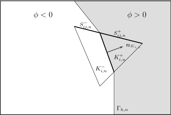
  Figure 2: Illustration of the two-medium fluid model.

• Numerical flux

  The numerical flux for the two-medium flow is composed of two parts: the cell edge flux and the interface flux. Below we explain the flux contribution towards any given cell $K_{i,n}$. We introduce two sets of flow variables at $n$-th time level

  $$\bm{U}_{K_{i,n}}^{\pm}=\left[\begin{array}[]{c}\rho_{K_{i,n}}^{\pm}\\ \rho_{K_{i,n}}^{\pm}\bm{u}_{K_{i,n}}^{\pm}\\ E_{K_{i,n}}^{\pm}\end{array}\right],$$

  which refer to the constant states in the cell $K_{i,n}^{\pm}$. Note that the flow variables vanish if there is no corresponding fluid in a given cell.

  • Cell edge flux

    The cell edge flux is the exchange of flux between the same fluid across the cell boundary. For any edge $S_{ij}$ of the cell $K_{i,n}$, let $\bm{n}_{ij,n}$ be the unit normal pointing from $K_{i,n}$ into the adjacent cell $K_{j,n}$. The cell edge flux across $S_{ij,n}^{\pm}$ is calculated as

    $$\hat{\bm{F}}_{ij,n}^{\pm}=\Delta t_{n}\left|S_{ij,n}^{\pm}\right|\hat{\bm{F}}\left(\bm{U}_{K_{i,n}}^{\pm},\bm{U}_{K_{j,n}}^{\pm};\bm{n}_{ij,n}\right),$$ (21)

    where $\Delta t_{n}$ denotes the current time step length, and $\hat{\bm{F}}(\bm{U}_{l},\bm{U}_{r};\bm{n})$ is a consistent monotonic numerical flux along $\bm{n}$. Here we adopt the local Lax-Friedrich flux

    $$\hat{\bm{F}}(\bm{U}_{l},\bm{U}_{r};\bm{n})=\dfrac{1}{2}\left(\bm{F}(\bm{U}_{l})+\bm{F}(\bm{U}_{r})\right)\cdot\bm{n}-\dfrac{1}{2}\lambda(\bm{U}_{r}-\bm{U}_{l}),$$

    where $\lambda$ is the maximal signal speed over $\bm{U}_{l}$ and $\bm{U}_{r}$.

  • Interface flux The interface flux is the exchange of the flux between two fluids due to the interaction of fluids at the interface. If $K_{i,n}$ is an interface cell, then the flux across the interface can be approximated by

    $$\hat{\bm{F}}_{K_{i,n}}^{\pm}=\Delta t_{n}\left|\Gamma_{K_{i,n}}\right|\begin{bmatrix}0\\ p_{K_{i,n}}^{*}\bm{n}_{K_{i,n}}\\ p_{K_{i,n}}^{*}u_{K_{i,n}}^{*}\end{bmatrix}.$$ (22)

    Here $p_{K_{i,n}}^{*}$ and $u_{K_{i,n}}^{*}$ are the interface pressure and normal velocity, which are obtained by applying the approximate solver we proposed in Section 3 to a local one-dimensional Riemann problem in the normal direction of the interface with initial states

    $$\begin{split}[\rho_{l},u_{l},p_{l}]^{\top}=[\rho_{K_{i,n}}^{-},\bm{u}_{K_{i,n}}^{-}\cdot\bm{n}_{K_{i,n}},p_{K_{i,n}}^{-}]^{\top},\\ [\rho_{r},u_{r},p_{r}]^{\top}=[\rho_{K_{i,n}}^{+},\bm{u}_{K_{i,n}}^{+}\cdot\bm{n}_{K_{i,n}},p_{K_{i,n}}^{+}]^{\top}.\end{split}$$

    Here the pressure $p_{K_{i,n}}^{\pm}$ in the initial states are given through the corresponding equations of state, namely

    $$p_{K_{i,n}}^{\pm}=P^{\pm}(\rho_{K_{i,n}}^{\pm},e_{K_{i,n}}^{\pm}),\quad e_{K_{i,n}}^{\pm}=\dfrac{E_{K_{i,n}}^{\pm}}{\rho_{K_{i,n}}^{\pm}}-\dfrac{1}{2}\|\bm{u}_{K_{i,n}}^{\pm}\|^{2}.$$

• Update of conservative variables

  Once the edge flux (21) and interface flux (22) are computed, the conservative variables at $(n+1)$-th time level is thus assigned as

  $$\bm{U}^{\pm}_{K_{i,n+1}}\!=\!\left\{\begin{array}[]{ll}\bm{0},&K^{\pm}_{i,n+1}\!=\!\varnothing,\\ \dfrac{1}{|K^{\pm}_{i,n+1}|}\!\left(|K^{\pm}_{i,n}|\bm{U}^{\pm}_{K_{i,n}}\!+\!\displaystyle\sum_{S_{ij}^{\pm}\subseteq\partial K_{i,n}^{\pm}}\hat{\bm{F}}_{ij,n}^{\pm}\!+\!\hat{\bm{F}}^{\pm}_{K_{i,n}}\right),&K^{\pm}_{i,n+1}\!\neq\!\varnothing.\end{array}\right.$$

Basically, the steps we presented above may close the numerical scheme, while there are more details in the practical implementation to gurantee the stability of the scheme. Please see [34] for those details.

5 Numerical Examples

In this section we present several numerical examples to validate our schemes, including one-dimensional Riemann problems, spherically symmetric problems and multi-dimensional shock impact problems. One-dimensional simulations are carried out on uniform interval meshes, while two and three-dimensional simulations are carried out on unstructured triangular and tetrahedral meshes respectively.

5.1 One-dimensional problems

In this part, we present some numerical examples of one-dimensional Riemann problems. The computational domain is $[0,1]$ with $400$ cells. And the reference solution, if mentioned, is computed on a very fine mesh with $10^{4}$ cells.

5.1.1 Shyue shock tube problem

This is a single-medium JWL Riemann problem used by Shyue [7]. The parameters of JWL EOS (27) therein are given by $A_{1}=8.545\times 10^{11}\,\mathrm{Pa},A_{2}=2.050\times 10^{10}\,\mathrm{Pa}$, $\omega=0.25$, $R_{1}=4.6$, $R_{2}=1.35$ and $\rho_{0}=1840\,\mathrm{kg/m^{3}}$. The initial conditions are

$$[\rho,u,p]^{\top}=\left\{\begin{array}[]{ll}[1700,~{}0,~{}10^{12}]^{\top},&x<0.5,\\[5.69054pt] [1000,~{}0,~{}5.0\times 10^{10}]^{\top},&x>0.5.\end{array}\right.$$

The simulation terminates at $t=1.2\times 10^{-5}$. In Fig. 3, the top panel shows the results of our numerical methods, while the bottom panel contains the results of Shyue [7]. Our results agree well with the highly resolved solution shown in a solid line given by Shyue.

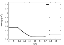
(a)

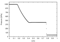
(b)

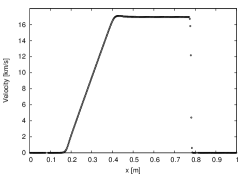
(c)

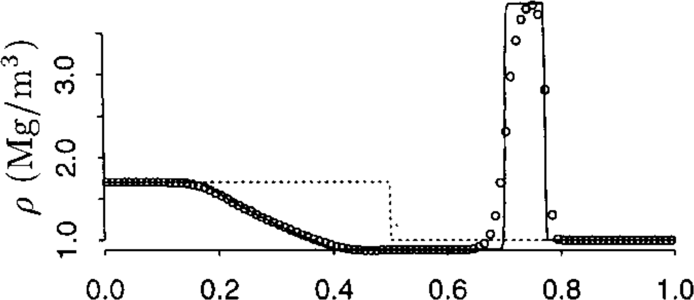
(a) Density

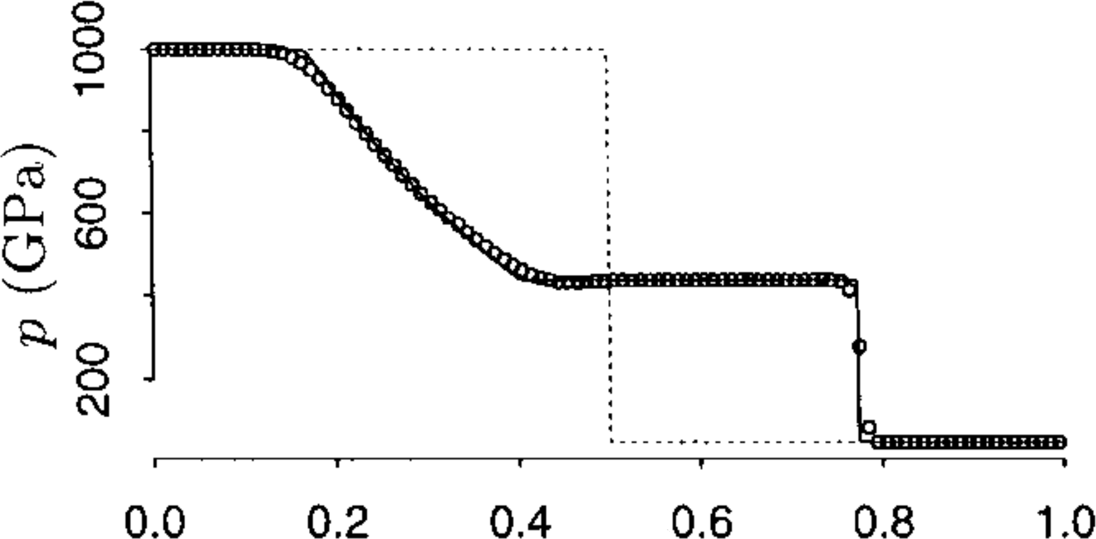
(b) Pressure

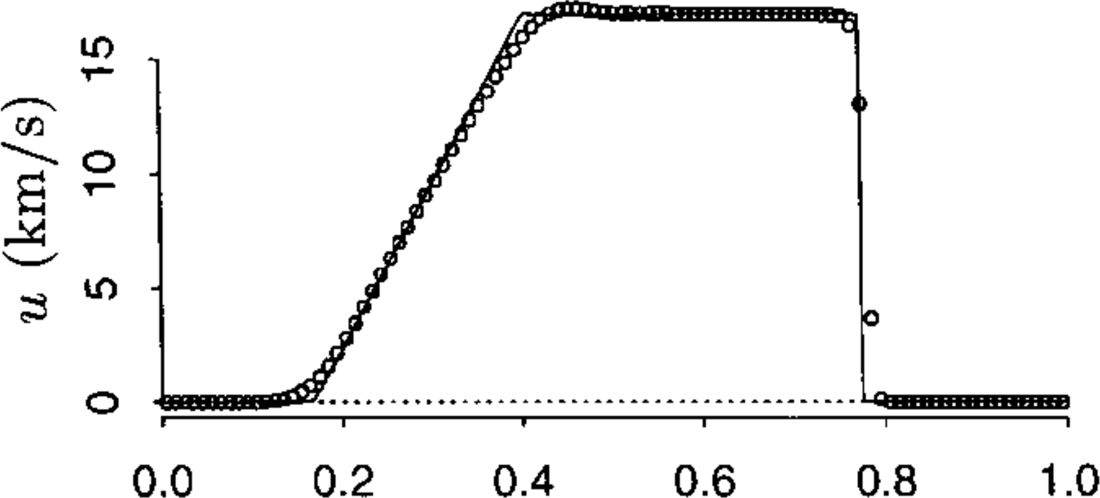
(c) Velocity

Figure 3: Shyue shock tube problem (top panel: our results, bottom panel: results from Shyue [7]).

5.1.2 Saurel shock tube problem

In this problem, we consider the advection of a density discontinuity of the liquid nitromethane described by Cochran-Chan EOS (28) in a uniform flow [2, 30]. The parameters are given by $A_{1}=8.192\times 10^{8}\,\mathrm{Pa}$, $A_{2}=1.508\times 10^{9}\,\mathrm{Pa},\omega=1.19$, $R_{1}=4.53$, $R_{2}=1.42$ and $\rho_{0}=1134\,\mathrm{kg/m^{3}}$. The initial value is

$$[\rho,u,p]^{\top}=\left\{\begin{array}[]{ll}[1134,~{}1000,~{}2.0\times 10^{10}]^{\top},&x<0.5,\\[5.69054pt] [500,~{}1000,~{}2.0\times 10^{10}]^{\top},&x>0.5.\end{array}\right.$$

The simulation terminates at $t=4.0\times 10^{-5}$. We use this Riemann problem to assess the performance of our methods against highly nonlinear equations of state. Fig. 4c displays the results of our numerical scheme and that of Saurel et al. [2], where we can see that there is no non-physical pressure and velocity across the contact discontinuity in our numerical scheme.

(a)

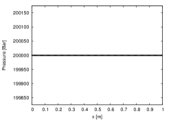
(b)

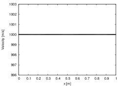
(c)

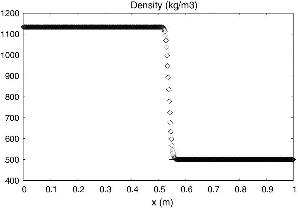
(a) Density

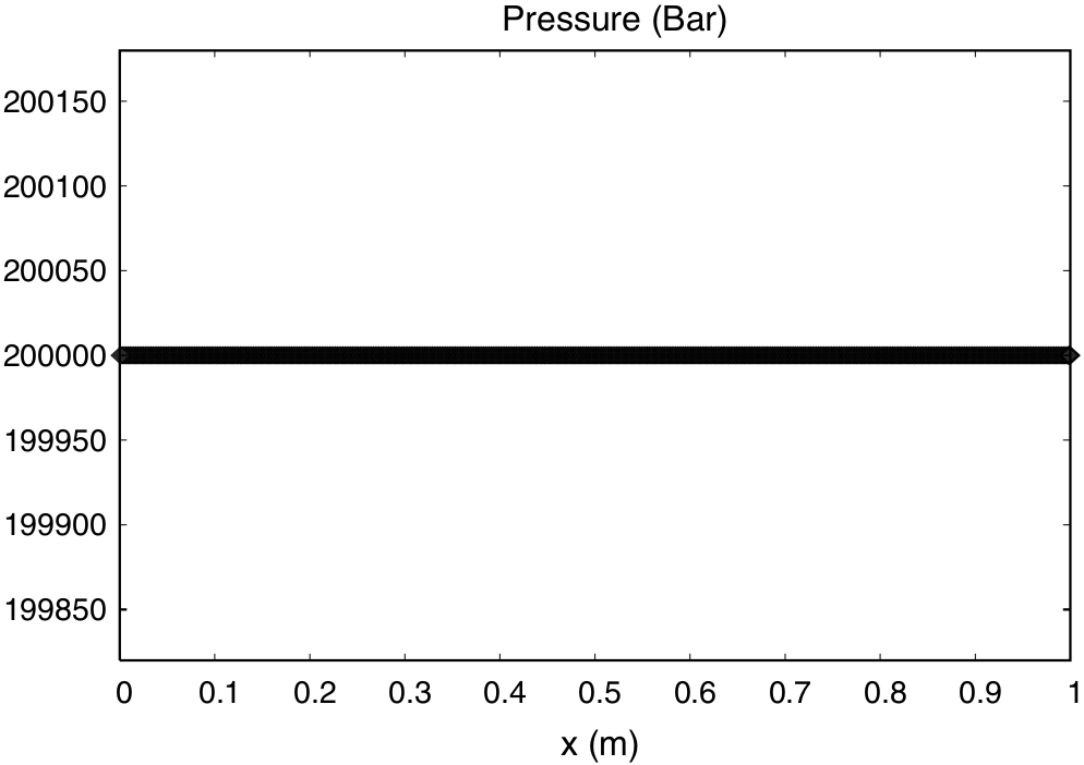
(b) Pressure

(c) Velocity

Figure 4: Saurel shock tube problem (top row: our results, bottom row: results from Saurel et al. [2]).

5.1.3 Ideal gas-water Riemann problem

In this example we simulate the ideal gas-water Riemann problems. The water is modeled by either the stiffened gas EOS (25) or the polynomial EOS (26). The initial density, velocity and pressure are both assigned with

$$[\rho,u,p]^{\top}=\left\{\begin{array}[]{ll}[1630,~{}0,~{}7.0\times 10^{9}]^{\top},&x<0.5,\\[5.69054pt] [1000,~{}0,~{}1.0\times 10^{5}]^{\top},&x>0.5.\end{array}\right.$$

The adiabatic exponent is $\gamma=2.0$ for the ideal gas EOS. The parameters of water are $\gamma=7.15$ and $p_{\infty}=3.31\times 10^{8}\,\mathrm{Pa}$ for the stiffened gas EOS [28, 51], and $\rho_{0}=1000\,\mathrm{kg/m^{3}}$, $A_{1}=2.20\times 10^{9}\,\mathrm{Pa}$, $A_{2}=9.54\times 10^{9}\,\mathrm{Pa}$, $A_{3}=1.45\times 10^{10}\,\mathrm{Pa}$, $B_{0}=B_{1}=0.28$, $T_{1}=2.20\times 10^{9}\,\mathrm{Pa}$ and $T_{2}=0$ for the polynomial EOS [52], respectively. The same parameters are chosen in the remaining numerical examples for the water.

The results with distinct equations of state at $t=8.0\times 10^{-5}$ are shown in Fig. 6, where we can observe that the numerical results agree well with the corresponding reference solutions. The comparison between these two graphs also shows the discrepancies due to the choices of the equations of state. It is observed that the shock wave in the stiffened gas EOS propagates faster than that in the polynomial EOS.

5.1.4 JWL-polynomial Riemann problem

This example concerns the JWL-polynomial Riemann problem. The initial states are

$$[\rho,u,p]^{\top}=\left\{\begin{array}[]{ll}[1630,~{}0,~{}8.3\times 10^{9}]^{\top},&x<0.5,\\[5.69054pt] [1000,~{}0,~{}1.0\times 10^{5}]^{\top},&x>0.5.\end{array}\right.$$

We use the following values to describe the TNT [53]: $A_{1}=3.712\times 10^{11}\,\mathrm{Pa}$, $A_{2}=3.230\times 10^{9}\,\mathrm{Pa}$, $\omega=0.30$, $R_{1}=4.15$, $R_{2}=0.95$ and $\rho_{0}=1630\,\mathrm{kg/m^{3}}$. The result at $t=8.0\times 10^{-5}$ is shown in Fig. 6, where we can observe that both the interface and shock are captured well without spurious oscillation.

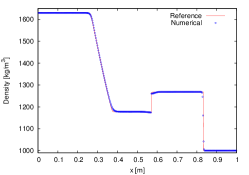
(a)

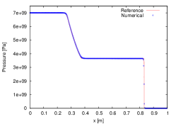
(b)

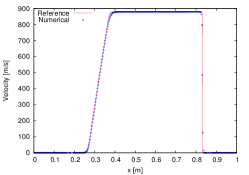
(c)

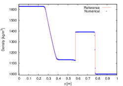
(a) Density

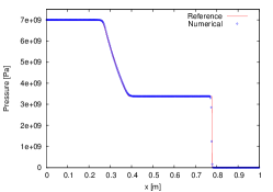
(b) Pressure

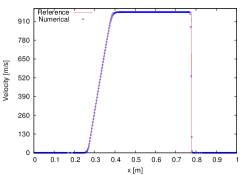
(c) Velocity

Figure 5: Ideal gas-water Riemann problem (top row: stiffened gas, bottom row: polynomial).

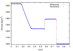
(a) Density

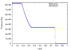
(b) Pressure

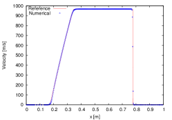
(c) Velocity

Figure 6: JWL-polynomial Riemann problem.

5.2 Spherically symmetric problems

In this part we present two spherically symmetric problems, where the governing equations are formulated as follows

$$\dfrac{\partial}{\partial t}\begin{bmatrix}r^{2}\rho\\ r^{2}\rho u\\ r^{2}E\end{bmatrix}+\dfrac{\partial}{\partial r}\begin{bmatrix}r^{2}\rho u\\ r^{2}(\rho u^{2}+p)\\ r^{2}(E+p)u\end{bmatrix}=\begin{bmatrix}0\\ 2rp\\ 0\end{bmatrix}.$$ (23)

The source term in (23) is discretized using an explicit Euler method.

5.2.1 Air blast problem

The shock wave that propagates through the air as a consequence of the nuclear explosion is commonly referred to as the blast wave. In this example we simulate the blast wave from one kiloton nuclear charge. The explosion products and air are modeled by the ideal gas EOS with adiabatic exponents $\gamma=1.2$ and $1.4$ respectively. The initial density and pressure are $618.935\,\mathrm{kg/m^{3}}$ and $6.314\times 10^{12}\,\mathrm{Pa}$ for the explosion products, and $1.29\,\mathrm{kg/m^{3}}$ and $1.013\times 10^{5}\,\mathrm{Pa}$ for the air. The initial interface is located at $r=0.3\,\mathrm{m}$ initially. To effectively capture the wave propagation we use a computational domain of radius $5000\,\mathrm{m}$.

It is known that the destructive effects of the blast wave can be measured by its overpressure, i.e., the amount by which the static pressure in the blast wave exceeds the ambient pressure ($1.013\times 10^{5}\,\mathrm{Pa}$). The overpressure increases rapidly to a peak value when the blast wave arrives, followed by a roughly exponential decay. The integration of the overpressure over time is called impulse. See Fig. 7 (a) for an illustration of these terminologies. Fig. 7 (b) – (d) show the peak overpressure, impulse and shock arrival time at different radii. The results are compared with the point explosion solutions in Qiao [54], which confirm the accuracy of our methods in the air blast applications.

5.2.2 Underwater explosion problem

We use this example to simulate the underwater explosion problem where a TNT of one hundred kilograms explodes in the water. The high explosives and water are characterized by the JWL EOS and polynomial EOS, respectively. The radii of the computational domain and the initial interface are $15\,\mathrm{m}$ and $0.245\,\mathrm{m}$ respectively. The initial pressure of the high explosives is $9.5\times 10^{9}\,\mathrm{Pa}$. The same problem has been simulated in [55] using ANSYS/AUTODYN. Fig. 8 shows the computed peak overpressure and impulse at different radii. The results agree well with the empirical law provided in [56].

(a) Typical pressure-time relation

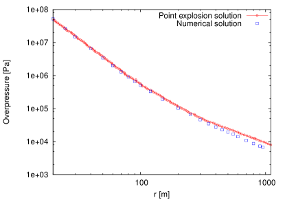
(b) Peak overpressure

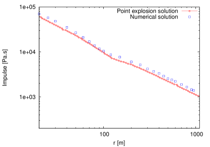
(c) Impulse

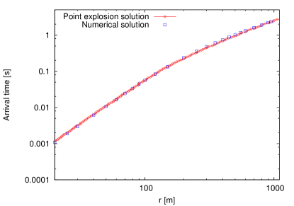
(d) Arrival time

Figure 7: Shock wave parameters for air blast problem.

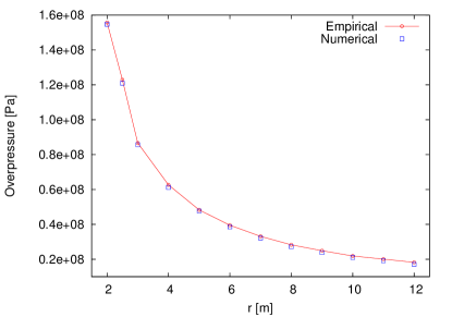
(a) Peak overpressure

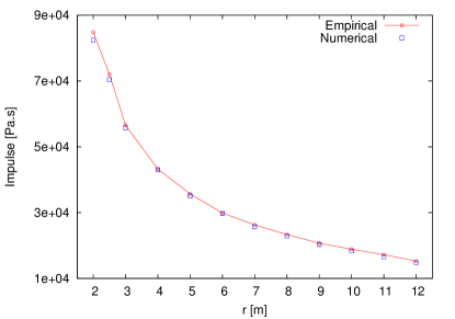
(b) Impulse

Figure 8: Shock wave parameters for underwater explosion problem.

5.3 Two-dimensional problems

In this part, we present a few two-dimensional cylindrically symmetric flows in engineering applications. The Euler equations for this configuration are formulated as a cylindrical form

$$\dfrac{\partial}{\partial t}\begin{bmatrix}r\rho\\ r\rho u\\ r\rho v\\ rE\end{bmatrix}+\dfrac{\partial}{\partial r}\begin{bmatrix}r\rho u\\ r(\rho u^{2}+p)\\ r\rho uv\\ r(E+p)u\end{bmatrix}+\dfrac{\partial}{\partial z}\begin{bmatrix}r\rho v\\ r\rho uv\\ r(\rho v^{2}+p)\\ r(E+p)v\end{bmatrix}=\begin{bmatrix}0\\ p\\ 0\\ 0\end{bmatrix}.$$

To improve the efficiency of the simulation, the $h$-adaptive mesh method is adopted here [49]. Roughly speaking, more elements will be distributed in the region where the jump of pressure is sufficiently large.

5.3.1 Nuclear air blast problem

In this example we simulate the nuclear air blast in the computational domain $0\leq r,z\leq 2000\,\mathrm{m}$. The initial states of the explosion products and air in this example are the same as that in Section 5.2.1, except that the bottom edge $z=0$ is now a rigid ground. The explosive center is located at the height $z=100\,\mathrm{m}$. And the radius of the initial interface is $0.3\,\mathrm{m}$ at $t=0$. Fig. 10 shows the pressure contours and adaptive meshes at $t=0.09\,\mathrm{s}$ and $0.3\,\mathrm{s}$. When the blast wave produced by the nuclear explosion arrives at the ground, it will be reflected firstly and propagate along the rigid ground simultaneously. When the incident angle exceeds the limit, the reflective wave switches from regular to irregular, and a Mach blast wave occurs. The peak overpressure and impulse at different radii are shown in Fig. 10. Our numerical results agree well the the reference data interpolated from the given standard data in [57].

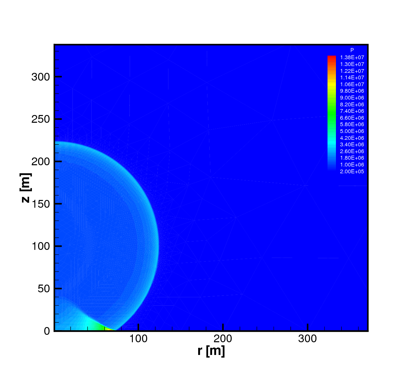
(a) Pressure contour at $t=0.09$s

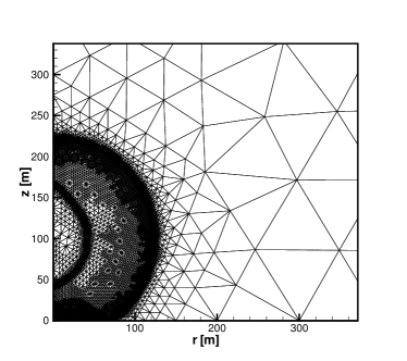
(b) Adaptive mesh at $t=0.09$s

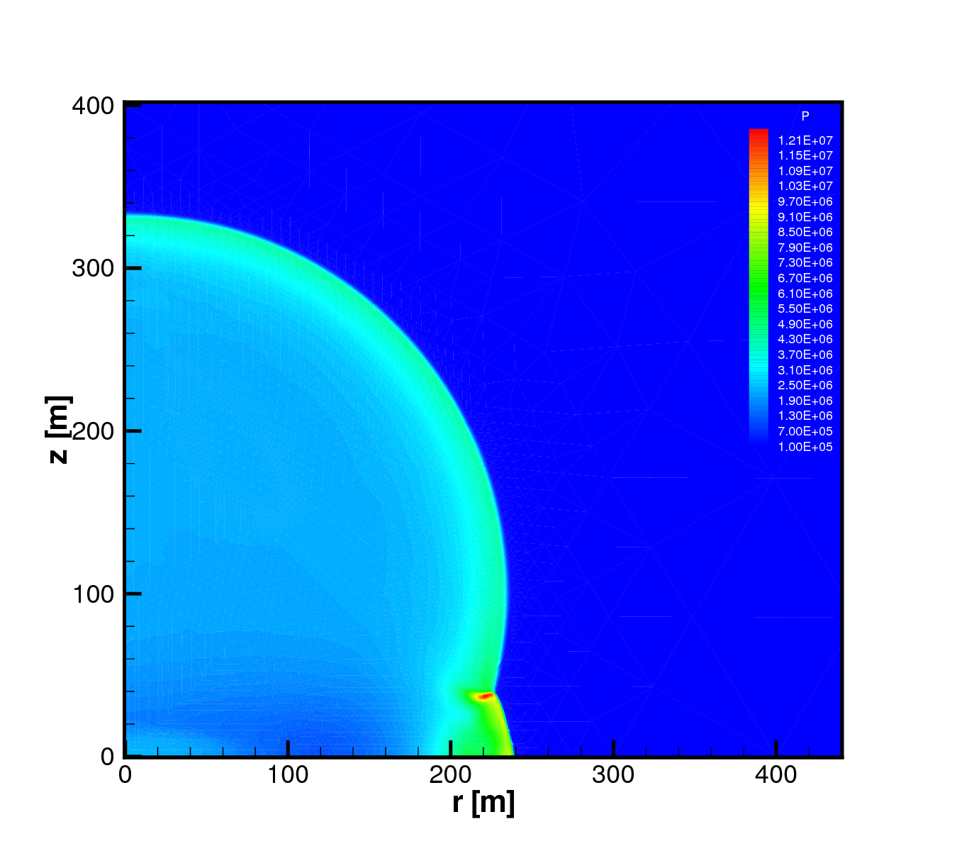
(c) Pressure contour at $t=0.3$s

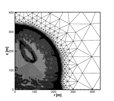
(d) Adaptive mesh at $t=0.3$s

Figure 9: Pressure contours and adaptive meshes for nuclear air blast problem.

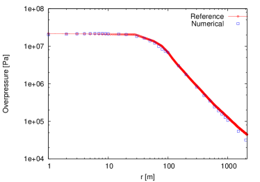
(a) Peak overpressure

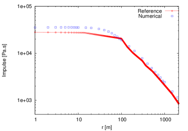
(b) Impulse

Figure 10: Shock wave parameters for nuclear air blast problem.

5.3.2 TNT explosion in air

We use this example to assess the isotropic behavior of TNT explosion in a computational domain $0\leq r\leq 20\,\mathrm{m},0\leq z\leq 40\,\mathrm{m}$. The initial density and pressure are $1630\,\mathrm{kg/m^{3}}$ and $9.5\times 10^{9}\,\mathrm{Pa}$ for high explosives, and $1.29\,\mathrm{kg/m^{3}}$ and $1.013\times 10^{5}\,\mathrm{Pa}$ for the air. The initial interface is a sphere of radius $0.0527\,\mathrm{m}$ centered at the height $z=10\,\mathrm{m}$. The results of shock produced by the high explosives are shown in Fig. 12. The shock parameters are shown in Fig. 12, in comparison with the experimental data in [58] and [59].

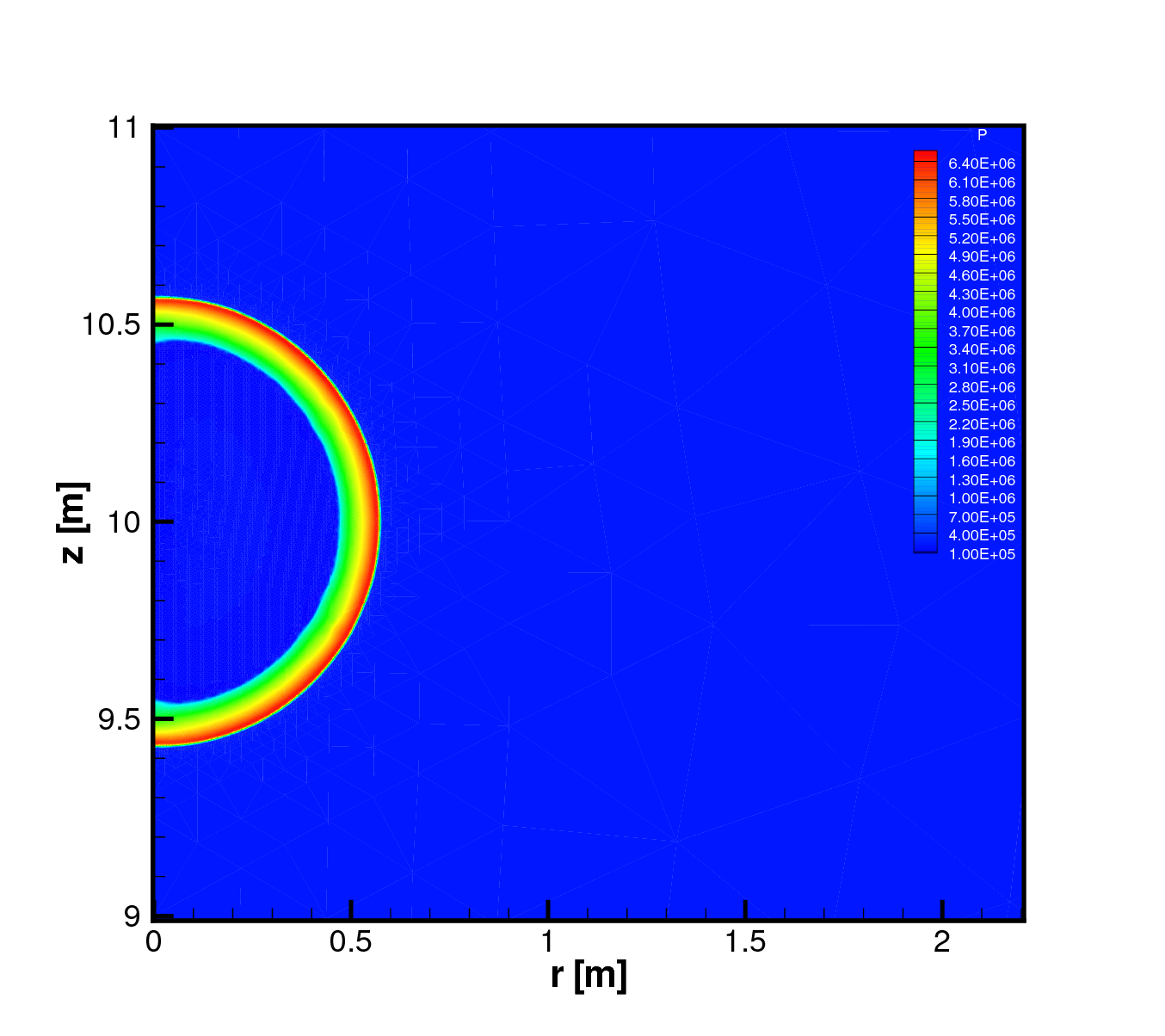
(a) Pressure contour at $t=1.8\times 10^{-4}$s

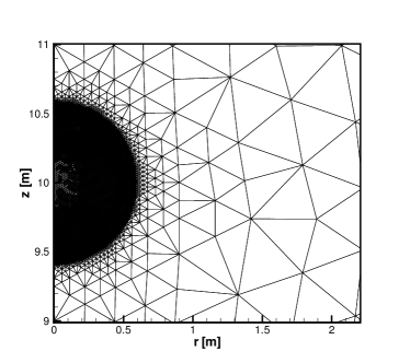
(b) Adaptive mesh at $t=1.8\times 10^{-4}$s

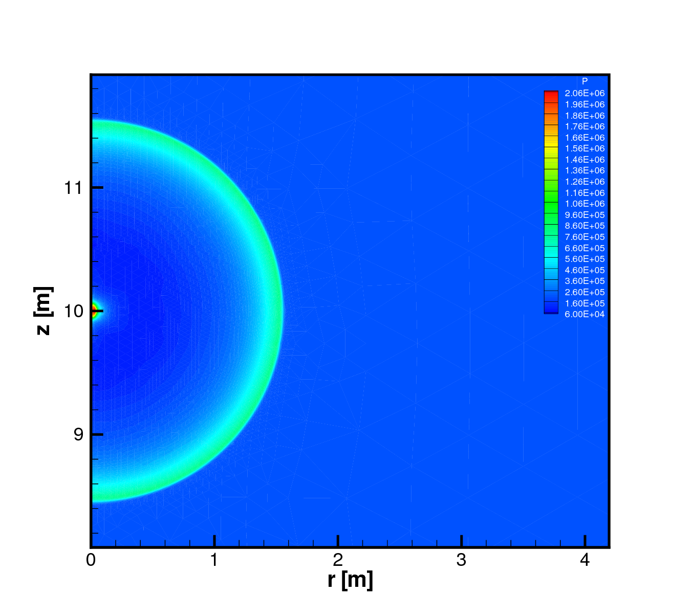
(c) Pressure contour at $t=1.2\times 10^{-3}$s

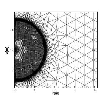
(d) Adaptive mesh at $t=1.2\times 10^{-3}$s

Figure 11: Pressure contours and adaptive meshes for TNT explosion in air.

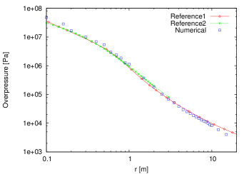
(a) Peak overpressure

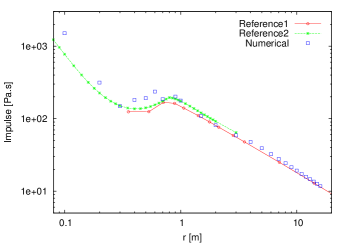
(b) Impulse

Figure 12: Shock wave parameters for TNT explosion in air. The reference solution 1 is taken from Baker [58], while the reference solution 2 is taken from Crowl [59].

5.4 Three-dimensional shock impact problem

In the last example, we present a three-dimensional shock impact problem in practical applications. The computational domain is a cross-shaped confined space $E_{1}\bigcup E_{2}$ where $E_{1}=[-2,2]\times[-2,2]\times[-6,6]$ and $E_{2}=[-6,6]\times[-2,2]\times[-2,2]$ in meters. The sphere of radius $0.4\,\mathrm{m}$ centered at the origin is filled with high explosives, while the remaining region is filled with air. The initial states are exactly the same as that of the problem in Section 5.3.2. Due to the symmetry we only compute the problem in the first octant, namely an L-shaped region. All the boundaries are reflective walls. Again we use the $h$-adaptive technique to capture the shock front. The total number of cells is about $0.8$ – $1$ million. To accelerate the computation we perform the parallel computing with eight processors based on the classical domain decomposition methods.

The numerical results of shock wave produced by the high explosives at $t=2.4\times 10^{-4}\,\mathrm{s}$ and $t=9.2\times 10^{-4}\,\mathrm{s}$ are displayed in Fig. 14. From here we can see that the shock wave propagates as an expansive spherical surface in earlier period. When the spherical shock wave impinges on the rigid surface, shock strength increases and shock reflection occurs. It is also observed in the slice plots of Fig. 14 that the wave structures are much more complicated in the three-dimensional confined space. The numerical results here also show the capability of our methods in resolving fully three-dimensional flows.

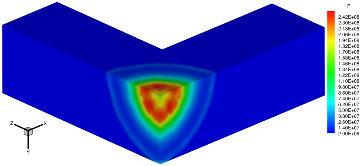
(a) Pressure contour at $t=2.4\times 10^{-4}$s

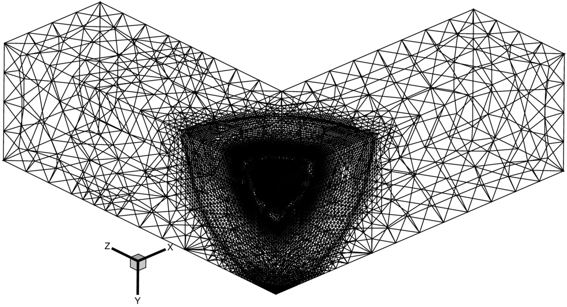
(b) Adaptive mesh at $t=2.4\times 10^{-4}$s

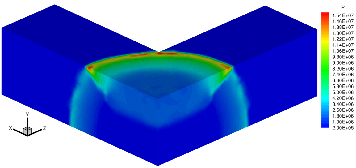
(c) Pressure contour at $t=9.2\times 10^{-4}$s

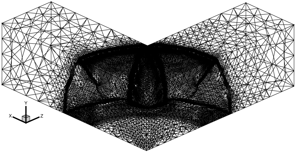
(d) Adaptive mesh at $t=9.2\times 10^{-4}$s

Figure 13: Pressure contours and adaptive meshes for three-dimensional shock impact problem. The plots (c) and (d) are turned over in the $y$-direction in order to display the shock reflection.

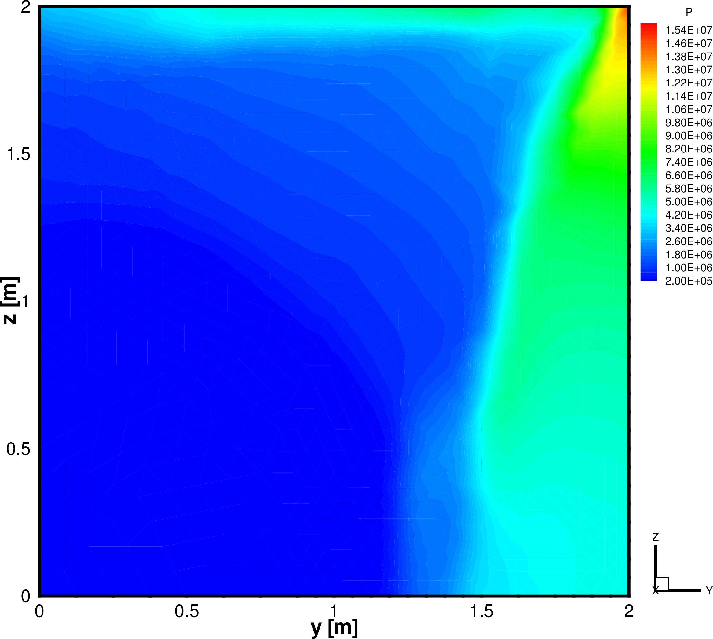
(a) Pressure slice at $x=2$m

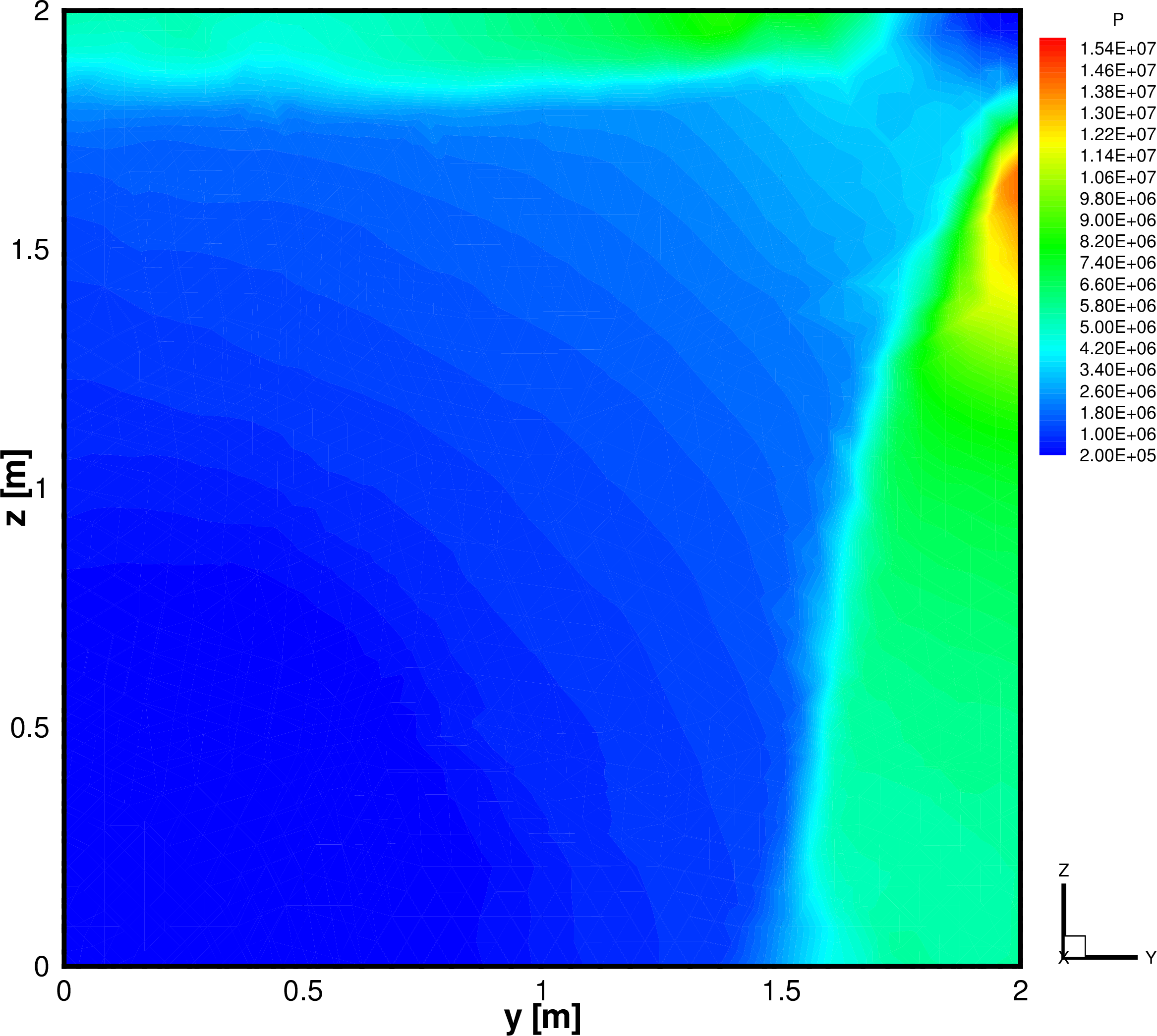
(b) Pressure slice at $x=2.2$m

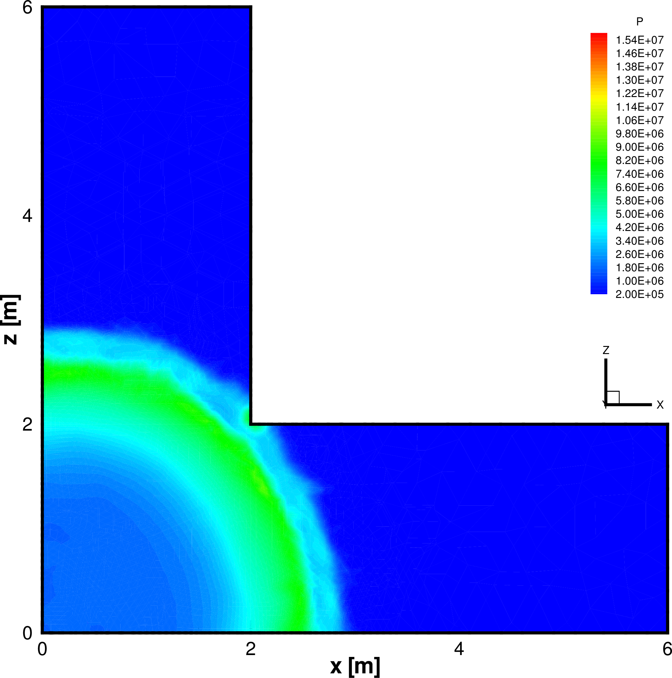
(c) Pressure slice at $y=1.8$m

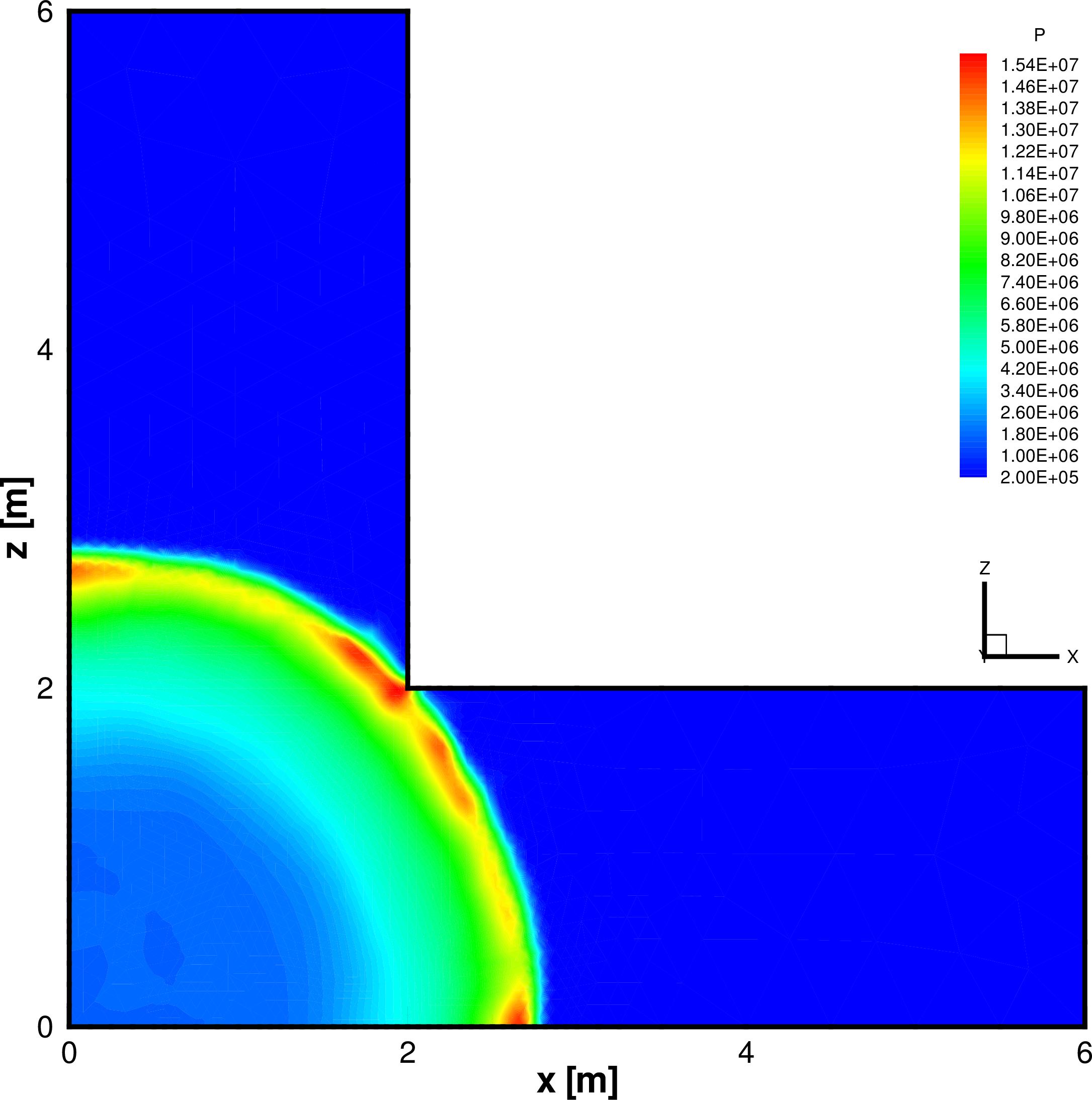
(d) Pressure slice at $y=2$m

Figure 14: Pressure slices at $t=9.2\times 10^{-4}$s.

6 Conclusions

We extend the numerical scheme in Guo et al. [34] to the fluids that obey a general Mie-Grüneisen equations of state. The algorithm of the multi-medium Riemann problem is elaborated, which is a fundamental element of the two-medium fluid flow. A variety of preliminary numerical examples and application problems validate the effectiveness and robustness of our methods. In our future work, we will generalize the framework to fluid-solid coupling problems.

Appendix A Collections of equations of state

In this appendix we elaborate the equations of state that are mentioned in the numerical results. For convenience, we also collect the expression of coefficients and their derivatives at the end of this part.

Ideal gas EOS

Most of gases can be modeled by the ideal gas law

$$p=(\gamma-1)\rho e,$$ (24)

where $\gamma>1$ is the adiabatic exponent.

Stiffened gas EOS

When considering water under high pressures, the following stiffened gas EOS is often used [28, 51]:

$$p=(\gamma-1)\rho e-\gamma p_{\infty},$$ (25)

where $\gamma>1$ is the adiabatic exponent, and $p_{\infty}$ is a constant.

Polynomial EOS

The polynomial EOS [52] can be used to model various materials

$$p=\begin{cases}A_{1}\mu+A_{2}\mu^{2}+A_{3}\mu^{3}+(B_{0}+B_{1}\mu)\rho_{0}e,&\mu>0,\\ T_{1}\mu+T_{2}\mu^{2}+B_{0}\rho_{0}e,&\mu\leq 0,\end{cases}$$ (26)

where $\mu={\rho}/{\rho_{0}}-1$ and $A_{1},A_{2},A_{3},B_{0},B_{1},T_{1},T_{2},\rho_{0}$ are positive constants. In this paper, we take an alternative formulation in the tension branch [60], where $p=T_{1}\mu+T_{2}\mu^{2}+(B_{0}+B_{1}\mu)\rho_{0}e$ for $\mu\leq 0$, to ensure the continuity of the speed of sound at $\mu=0$. Such a formulation avoids the occurance of anomalous waves in the Riemann problem, which does not exist in real physics. When $B_{1}\leq B_{0}\leq B_{1}+2$ and $T_{1}\geq 2T_{2}$, the polynomial EOS satisfies the conditions (C1) and (C3). In addition, if the density $\rho\geq{B_{0}\rho_{0}}/{(B_{1}+2)}$, then the polynomial EOS also satisfies the condition (C2).

JWL EOS

Various detonation products of high explosives can be characterized by the JWL EOS [53]

$$p=A_{1}\left(1-\frac{\omega\rho}{R_{1}\rho_{0}}\right)\exp\left(-\frac{R_{1}\rho_{0}}{\rho}\right)+A_{2}\left(1-\frac{\omega\rho}{R_{2}\rho_{0}}\right)\exp\left(-\frac{R_{2}\rho_{0}}{\rho}\right)+\omega\rho e,$$ (27)

where $A_{1},A_{2},\omega,R_{1},R_{2}$ and $\rho_{0}$ are positive constants. Obviously the JWL EOS (27) satisfies the conditions (C1) and (C2). To enforce the condition (C3) we first notice that

$$\lim_{\rho\rightarrow 0^{+}}h^{\prime}(\rho)=0.$$

Then it suffices to ensure that $h^{\prime\prime}(\rho)\geq 0$, which is equivalent to the following inequality in terms of $\nu=\rho_{0}/\rho$:

$$R_{1}\nu-2-\omega\geq G(\nu):=\dfrac{A_{2}R_{2}}{A_{1}R_{1}}(2+\omega-R_{2}\nu)\exp((R_{1}-R_{2})\nu).$$

A simple calculus shows that the maximum value of the function $G(\nu)$ above is given by

$$\alpha=\dfrac{A_{2}R_{2}^{2}}{A_{1}R_{1}(R_{1}-R_{2})}\exp\left(\dfrac{(2+\omega)(R_{1}-R_{2})-R_{2}}{R_{2}}\right).$$

Therefore a sufficient condition for (C3) is that the density satisfies

$$\rho\leq\dfrac{R_{1}}{2+\omega+\alpha}\rho_{0},$$

which is valid for most cases.

Cochran-Chan EOS

The Cochran-Chan EOS is commonly used to describe the reactants of condensed phase explosives [2, 30], which can be formulated as

$$p=\dfrac{A_{1}(R_{1}-1-\omega)}{R_{1}-1}\left(\dfrac{\rho}{\rho_{0}}\right)^{R_{1}}-\dfrac{A_{2}(R_{2}-1-\omega)}{R_{2}-1}\left(\dfrac{\rho}{\rho_{0}}\right)^{R_{2}}+\omega\rho e,$$ (28)

where $A_{1},A_{2},\omega,R_{1},R_{2}$ and $\rho_{0}$ are positive constants. The Cochran-Chan EOS satisfies the conditions (C1), (C2) and (C3) if $1<R_{2}\leq 1+\omega\leq R_{1}$.

Table 1: *

List of coefficients and their derivatives for several equations of state. Ideal Stiffened Polynomial JWL Cochran-Chan $\varGamma(\rho)$ $\gamma-1$ $\gamma-1$ $B_{1}+{(B_{0}-B_{1})\rho_{0}}/{\rho}$ $\omega$ $\omega$ $\varGamma^{\prime}(\rho)$ $0$ $0$ $-{(B_{0}-B_{1})\rho_{0}}/{\rho^{2}}$ $0$ $0$ $\varGamma^{\prime\prime}(\rho)$ $0$ $0$ ${2(B_{0}-B_{1})\rho_{0}}/{\rho^{3}}$ $0$ $0$ $h(\rho)$ $0$ $-\gamma p_{\infty}$ $\begin{cases}A_{1}\mu+A_{2}\mu^{2}+A_{3}\mu^{3},&\rho>\rho_{0}\\ T_{1}\mu+T_{2}\mu^{2},&\rho\leq\rho_{0}\end{cases}$ $A_{1}\left(1-\dfrac{\omega\rho}{R_{1}\rho_{0}}\right)\exp\left(-\dfrac{R_{1}\rho_{0}}{\rho}\right)$ $+A_{2}\left(1-\dfrac{\omega\rho}{R_{2}\rho_{0}}\right)\exp\left(-\dfrac{R_{2}\rho_{0}}{\rho}\right)$ $\dfrac{A_{1}(R_{1}-1-\omega)}{R_{1}-1}\left(\dfrac{\rho}{\rho_{0}}\right)^{R_{1}}$ $-\dfrac{A_{2}(R_{2}-1-\omega)}{R_{2}-1}\left(\dfrac{\rho}{\rho_{0}}\right)^{R_{2}}$ $h^{\prime}(\rho)$ $0$ $0$ $\begin{cases}(A_{1}+2A_{2}\mu+3A_{3}\mu^{2})/\rho_{0},&\rho>\rho_{0}\\ (T_{1}+2T_{2}\mu)/\rho_{0},&\rho\leq\rho_{0}\end{cases}$ $A_{1}\left(\dfrac{R_{1}\rho_{0}}{\rho^{2}}-\dfrac{\omega}{\rho}-\dfrac{\omega}{R_{1}\rho_{0}}\right)\exp\left(-\dfrac{R_{1}\rho_{0}}{\rho}\right)$ $+A_{2}\left(\dfrac{R_{2}\rho_{0}}{\rho^{2}}-\dfrac{\omega}{\rho}-\dfrac{\omega}{R_{2}\rho_{0}}\right)\exp\left(-\dfrac{R_{2}\rho_{0}}{\rho}\right)$ $\dfrac{A_{1}R_{1}(R_{1}-1-\omega)}{R_{1}-1}\left(\dfrac{\rho}{\rho_{0}}\right)^{R_{1}-1}$ $-\dfrac{A_{2}R_{2}(R_{2}-1-\omega)}{R_{2}-1}\left(\dfrac{\rho}{\rho_{0}}\right)^{R_{2}-1}$ $h^{\prime\prime}(\rho)$ $0$ $0$ $\begin{cases}(2A_{2}+6A_{3}\mu)/\rho_{0}^{2},&\rho>\rho_{0}\\ 2T_{2}/\rho_{0}^{2},&\rho\leq\rho_{0}\end{cases}$ $\dfrac{A_{1}R_{1}\rho_{0}}{\rho^{3}}\left(\dfrac{R_{1}\rho_{0}}{\rho}-2-\omega\right)\exp\left(-\dfrac{R_{1}\rho_{0}}{\rho}\right)$ $+\dfrac{A_{2}R_{2}\rho_{0}}{\rho^{3}}\left(\dfrac{R_{2}\rho_{0}}{\rho}-2-\omega\right)\exp\left(-\dfrac{R_{2}\rho_{0}}{\rho}\right)$ ${A_{1}R_{1}(R_{1}-1-\omega)}\left(\dfrac{\rho}{\rho_{0}}\right)^{R_{1}-2}$ $-{A_{2}R_{2}(R_{2}-1-\omega)}\left(\dfrac{\rho}{\rho_{0}}\right)^{R_{2}-2}$

References

References

• [1] R. Abgrall. How to prevent pressure oscillations in multicomponent flow calculations: a quasi conservative approach. Journal of Computational Physics, 125(1):150–160, 1996.
• [2] R. Saurel, E. Franquet, E. Daniel, and O.L. Metayer. A relaxation-projection method for compressible flows. Part I: The numerical equation of state for the Euler equations. Journal of Computational Physics, 223(2):822–845, 2007.
• [3] T.G. Liu, B.C. Khoo, and K.S. Yeo. Ghost fluid method for strong shock impacting on material interface. Journal of Computational Physics, 190(2):651–681, 2003.
• [4] R. Abgrall and S. Karni. Computations of compressible multifluids. Journal of Computational Physics, 169(2):594–623, 2001.
• [5] S. Karni. Multicomponent flow calculations by a consistent primitive algorithm. Journal of Computational Physics, 112(1):31–43, 1994.
• [6] M. Arienti, E. Morano, and J.E. Shepherd. Shock and detonation modeling with the Mie-Grüneisen equation of state. Technical report, California Institute of Technology, 2004.
• [7] K.-M. Shyue. A fluid-mixture type algorithm for compressible multicomponent flow with Mie–Grüneisen equation of state. Journal of Computational Physics, 171(2):678–707, 2001.
• [8] R. Saurel and R. Abgrall. A simple method for compressible multifluid flows. SIAM Journal on Scientific Computing, 21(3):1115–1145, 1999.
• [9] M.A. Price, V.T. Nguyen, O. Hassan, and K. Morgan. A method for compressible multimaterial flows with condensed phase explosive detonation and airblast on unstructured grids. Computers &amp; Fluids, 111:76–90, 2015.
• [10] R. Saurel, F. Petitpas, and R.A. Berry. Simple and efficient relaxation methods for interfaces separating compressible fluids, cavitating flows and shocks in multiphase mixtures. Journal of Computational Physics, 228(5):1678–1712, 2009.
• [11] F. Petitpas, J. Massoni, and R. Saurel. Diffuse interface model for high speed cavitating underwater systems. International Journal of Multiphase Flow, 35(8):747–759, 2009.
• [12] M.R. Ansari and A. Daramizadeh. Numerical simulation of compressible two-phase flow using a diffuse interface method. International Journal of Heat and Fluid Flow, 42(8):209–223, 2013.
• [13] R. Scardovelli and S. Zaleski. Direct numerical simulation of free-surface and interfacial flow. Annual Review of Fluid Mechanics, 31(1):567–603, 1999.
• [14] W.F. Noh and P. Woodward. SLIC (simple line interface calculation). In Proceedings of the Fifth International Conference on Numerical Methods in Fluid Dynamics, pages 330–340. Springer, 1976.
• [15] J.A. Sethian. Evolution, implementation, and application of level set and fast marching methods for advancing fronts. Journal of Computational Physics, 169(2):503–555, 2001.
• [16] M. Sussman, P. Smereka, and S. Osher. A level set approach for computing solutions to incompressible two-phase flow. Journal of Computational Physics, 114(1):146–159, 1994.
• [17] H.T. Ahn and M. Shashkov. Multi-material interface reconstruction on generalized polyhedral meshes. Journal of Computational Physics, 226(2):2096–2132, 2007.
• [18] V. Dyadechko and M. Shashkov. Reconstruction of multi-material interfaces from moment data. Journal of Computational Physics, 227(11):5361–5384, 2008.
• [19] H.R. Anbarlooei and K. Mazaheri. Moment of fluid interface reconstruction method in multi-material arbitrary Lagrangian Eulerian (MMALE) algorithms. Computer Methods In Applied Mechanics And Engineering, 198(47):3782–3794, 2009.
• [20] J. Glimm, J.W. Grove, and X.L. Li. Three-dimensional front tracking. SIAM Journal on Scientific Computing, 19(3):1703–727, 1998.
• [21] G. Tryggvason, B. Bunner, and A. Esmaeeli. A front-tracking method for the computations of multiphase flow. Journal of Computational Physics, 169(2):708–759, 2001.
• [22] S.K. Godunov, A.V. Zabrodin, M.I. Ivanov, A.N. Kraiko, and G.P. Prokopov. Numerical solution of multidimensional problems of gas dynamics. Moscow Izdatel Nauka, 1, 1976.
• [23] B.J. Plohr. Shockless acceleration of thin plates modeled by a tracked random choice method. Journal of American Institute of Aeronautics and Astronautics, 26(4):470–478, 1988.
• [24] J.J. Gottlieb and C.P.T. Groth. Assessment of Riemann solvers for unsteady one-dimensional inviscid flows of perfect gases. Journal of Computational Physics, 78(2):437–458, 1988.
• [25] E.F. Toro. Riemann Solver and Numerical Methods for Fluid Dynamics. Springer, 2008.
• [26] M. Larini, R. Saurel, and J.C. Loraud. An exact Riemann solver for detonation products. Shock Waves, 2(4):225–236, 1992.
• [27] L. Quartapelle, L. Castelletti, A. Guardone, and G. Quaranta. Solution of the Riemann problem of classical gasdynamics. Journal of Computational Physics, 190(1):118–140, 2003.
• [28] A.S.D. Rallu. A Multiphase Fluid-Structure Computational Framework for Underwater Implosion Problems. PhD thesis, Stanford University, 2009.
• [29] C. Farhat, J.F.D.R. Gerbeau, and A.Rallu. FIVER: A finite volume method based on exact two-phase Riemann problems and sparse grids for multi-material flows with large density jumps. Journal of Computational Physics, 231(19):6360–6379, 2012.
• [30] B.J. Lee, E.F. Toro, C.E. Castro, and N.Nikiforakis. Adaptive Osher-type scheme for the Euler equations with highly nonlinear equations of state. Journal of Computational Physics, 246:165–183, 2013.
• [31] J.W. Banks. On exact conservation for the Euler equations with complex equations of state. Communications in Computational Physics, 8(5):995, 2010.
• [32] J.R. Kamm. Solution of the 1D Riemann problem with a general EOS in ExactPack. In 4th ASME Conference on Verification and Validation of Simulations, Las Vegas, NV, 2015.
• [33] R.S. Dembo, S.C. Eisenstat, and T. Steihaug. Inexact Newton methods. SIAM Journal on Numerical Analysis, 19(2):400–408, 1982.
• [34] Y. Guo, R. Li, and C. Yao. A numerical method on Eulerian grids for two-phase compressible flow. Advances in Applied Mathematics and Mechanics, 8(2):187–212, 2016.
• [35] O. Heuzé. General form of the Mie–Grüneisen equation of state. Comptes Rendus Mecanique, 340(10):679–687, 2012.
• [36] R.G. Smith. The Riemann problem in gas dynamics. Transactions of the American Mathematical Society, 249(1):1–50, 1979.
• [37] R. Menikoff and B.J. Plohr. The Riemann problem for fluid flow of real materials. Reviews of Modern Physics, 61:75–130, January 1989.
• [38] P.A. Thompson. A fundamental derivative in gasdynamics. The Physics of Fluids, 14(9):1843–1849, 1971.
• [39] H. Weyl. Shock waves in arbitrary fluids. Communications on Pure and Applied Mathematics, 2(2-3):103–122, 1949.
• [40] P.A. Thompson and K.C. Lambrakis. Negative shock waves. Journal of Fluid Mechanics, 60(1):187–208, 1973.
• [41] T.P. Liu. The Riemann problem for general systems of conservation laws. Journal of Differential Equations, 18(1):218–234, 1975.
• [42] T.P. Liu. The entropy condition and the admissibility of shocks. Journal of Mathematical Analysis and Applications, 53(1):78–88, 1976.
• [43] R.L. Pego. Nonexistence of a shock layer in gas dynamics with a nonconvex equation of state. Archive for Rational Mechanics and Analysis, 94(2):165–178, 1986.
• [44] H.A. Bethe. On the theory of shock waves for an arbitrary equation of state. In Classic Papers in Shock Compression Science, pages 421–495. Springer, 1998.
• [45] J.W. Bates. Studies of non-classical shock wave phenomena. Shock Waves, 12(1):31–37, 2002.
• [46] A. Voss and W. Dahmen. Exact Riemann solution for the Euler equations with nonconvex and nonsmooth equation of state. Technical report, Fakultät für Mathematik, Informatik und Naturwissenschaften, 2005.
• [47] S. Müller and A. Voss. The Riemann problem for the Euler equations with nonconvex and nonsmooth equation of state: construction of wave curves. SIAM Journal on Scientific Computing, 28(2):651–681, 2006.
• [48] M. Fossati and L. Quartapelle. The Riemann problem of the Euler equations for classical and nonclassical fluids. Department of Aerospace Science and Technology, 38(3):640–658, 2014.
• [49] R. Li and S. Wu. $h$-adaptive mesh method with double tolerance adaptive strategy for hyperbolic conservation laws. Journal of Scientific Computing, 56(3):616–636, 2013.
• [50] Y. Di, R. Li, T. Tang, and P. Zhang. Level set calculations for incompressible two-phase flows on a dynamically adaptive grid. Journal of Scientific Computing, 31(1):75–98, 2007.
• [51] C. Wang, H. Tang, and T. Liu. An adaptive ghost fluid finite volume method for compressible gas–water simulations. Journal of Computational Physics, 227(12):6385–6409, 2008.
• [52] N. Jha and B.S.K. Kumar. Under water explosion pressure prediction and validationa using ANSYS/AUTODYN. International Journal of Science and Research, 3:1162–1165, 2014.
• [53] R.W. Smith. AUSM (ALE): a geometrically conservative arbitrary Lagrangian–Eulerian flux splitting scheme. Journal of Computational Physics, 150(1):268–286, 1999.
• [54] D.J. Qiao. An Introduction to Nuclear Explosion Physics. National Defence Industry Press (in Chinese), 2003.
• [55] X. Jia. Numerical Simulation of Underwater Explosion and Its Effect on Structures Based on Commercial Softwares (in Chinese). PhD thesis, Nanjing University of Technology and Engineering, 2008.
• [56] R.H. Cole and R. Weller. Underwater explosions. Physics Today, 1:35, 1948.
• [57] S. Glasstone and P.J. Dolan. Effects of nuclear weapons. Technical report, Department of Defense, Washington, DC (USA); Department of Energy, Washington, DC (USA), 1977.
• [58] W.E. Baker. Explosions in Air. University of Texas Press, 1973.
• [59] W.K. Crowl. Structures to resist the effects of accidental explosions. Technical report, US Army, Navy and Air Force, US Government Printing Office, Washington DC, 1969.
• [60] N.N. Autodyn. Theory manual. Technical report, Horsham, UK: Century Dynamics Ltd, 2003.