Infrared Fixed Point Physics in ${\rm SO}(N_{c})$ and ${\rm Sp}(N_{c})$ Gauge Theories

Abstract

We study properties of asymptotically free vectorial gauge theories with gauge groups $G={\rm SO}(N_{c})$ and $G={\rm Sp}(N_{c})$ and $N_{f}$ fermions in a representation $R$ of $G$, at an infrared (IR) zero of the beta function, $\alpha_{IR}$, in the non-Abelian Coulomb phase. The fundamental, adjoint, and rank-2 symmetric and antisymmetric tensor fermion representations are considered. We present scheme-independent calculations of the anomalous dimensions of (gauge-invariant) fermion bilinear operators $\gamma_{\bar{\psi}\psi,IR}$ to $O(\Delta_{f}^{4})$ and of the derivative of the beta function at $\alpha_{IR}$, denoted $\beta^{\prime}_{IR}$, to $O(\Delta_{f}^{5})$, where $\Delta_{f}$ is an $N_{f}$-dependent expansion variable. It is shown that all coefficients in the expansion of $\gamma_{\bar{\psi}\psi,IR}$ that we calculate are positive for all representations considered, so that to $O(\Delta_{f}^{4})$, $\gamma_{\bar{\psi}\psi,IR}$ increases monotonically with decreasing $N_{f}$ in the non-Abelian Coulomb phase. Using this property, we give a new estimate of the lower end of this phase for some specific realizations of these theories.

I Introduction

The evolution of an asymptotically free gauge theory from the ultraviolet (UV) to the infrared is of fundamental importance. The evolution of the running gauge coupling $g=g(\mu)$, as a function of the Euclidean momentum scale, $\mu$, is described by the renormalization-group (RG) beta function, $\beta_{g}=dg/dt$, or equivalently, $\beta_{\alpha}=d\alpha/dt$, where $\alpha(\mu)=g(\mu)^{2}/(4\pi)$ and $dt=d\ln\mu$ (the argument $\mu$ will often be suppressed in the notation). The asymptotic freedom (AF) property means that the gauge coupling approaches zero in the deep UV, which enables one to perform reliable perturbative calculations in this regime. Here we consider a vectorial, asymptotically free gauge theory (in four spacetime dimensions) with two types of gauge groups, namely the orthogonal group, $G={\rm SO}(N_{c})$, and the symplectic group (with even $N_{c}$), $G={\rm Sp}(N_{c})$, and $N_{f}$ copies (“flavors”) of Dirac fermions transforming according to the respective (irreducible) representations $R$ of the gauge group, where $R$ is the fundamental ($F$), adjoint ($A$), or rank-2 symmetric ($S_{2}$) or antisymmetric ($A_{2}$) tensor. It may be recalled that for SO($N_{c})$, the adjoint and $A_{2}$ representations are equivalent, while for Sp($N_{c})$, the adjoint and $S_{2}$ representations are equivalent. For technical convenience, we take the fermions to be massless fm . In the case of SO($N_{c}$), we do not consider $N_{c}=2$, since ${\rm SO}(2)\cong{\rm U}(1)$, and a U(1) gauge theory is not asymptotically free (but instead is infrared-free).

If $N_{f}$ is sufficiently large (but less than the upper limit implied by asymptotic freedom), then the beta function has an IR zero, at a coupling denoted $\alpha_{IR}$, that controls the UV to IR evolution b1 ; b2 . Given that this is the case, as the Euclidean scale $\mu$ decreases from the UV to the IR, $\alpha(\mu)$ increases toward the limiting value $\alpha_{IR}$, and the IR theory is in a chirally symmetric (deconfined) non-Abelian Coulomb phase (NACP) sksb . Here the value $\alpha=\alpha_{IR}$ is an exact IR fixed point of the renormalization group, and the corresponding theory in this IR limit is scale-invariant and generically also conformal invariant scalecon .

The physical properties of the conformal field theory at $\alpha_{IR}$ are of considerable interest. These properties clearly cannot depend on the scheme used for the regularization and renormalization of the theory. (We restrict here to mass-independent schemes.) In usual perturbative calculations, one computes a given quantity as a series expansion in powers of $\alpha$ to some finite $n$-loop order. With this procedure, the result is scheme-dependent beyond the leading term(s). For example, the beta function is scheme-dependent at loop order $\ell\geq 3$ and the terms in an anomalous dimension are scheme-dependent at loop order $\ell\geq 2$ gross75 . This applies, in particular, to the evaluation at an IR fixed point. A key fact is that as $N_{f}$ (considered to be extended from positive integers to positive real numbers) approaches the upper limit allowed by the requirement of asymptotic freedom, denoted $N_{u}$ (given in Eq. (9) below), it follows that $\alpha_{IR}\to 0$. Consequently, one can express a physical quantity evaluated at $\alpha_{IR}$ in a manifestly scheme-independent way as a series expansion in powers of the variable

$$\Delta_{f}=N_{u}-N_{f}\ .$$ (1)

For values of $N_{f}$ in the non-Abelian Coulomb phase such that $\Delta_{f}$ is not too large, one may expect this expansion to yield reasonably accurate perturbative calculations of physical quantities at $\alpha_{IR}$ bz . Some early work on this type of expansion was reported in bz ; gkgg . In gtr -dexl we have presented scheme-independent calculations of a number of physical quantities at an IR fixed point in an asymptotically free vectorial gauge theory with a general (simple) gauge group $G$ and $N_{f}$ massless fermions in a representation $R$ of $G$, including the anomalous dimension of a (gauge-invariant) bilinear fermion operator up to $O(\Delta_{f}^{4})$ and the derivative of the beta function at $\alpha_{IR}$, $\frac{d\beta}{d\alpha}|_{\alpha=\alpha_{IR}}\equiv\beta^{\prime}_{IR}$, up to $O(\Delta_{f}^{5})$. These results for general $G$ and $R$ were evaluated for $G={\rm SU}(N_{c})$ with several fermion representations. Since the global chiral symmetry is realized exactly in the non-Abelian Coulomb phase, the bilinear fermion operators can be classified according to their representation properties under this symmetry, including flavor-singlet and flavor-nonsinglet. Let $\gamma_{\bar{\psi}\psi}$ denote the anomalous dimension of the (gauge-invariant) fermion bilinear, $\bar{\psi}\psi$ and let $\gamma_{\bar{\psi}\psi,IR}$ denote its value at the IR fixed point. The scheme-independent expansion of $\gamma_{\bar{\psi}\psi,IR}$ can be written as

$$\gamma_{\bar{\psi}\psi,IR}=\sum_{j=1}^{\infty}\kappa_{j}\,\Delta_{f}^{\ j}\ .$$ (2)

We denote the truncation of right-hand side of Eq. (2) so the upper limit on the sum over $j$ is the maximal power $p$ rather than $\infty$ as $\gamma_{\bar{\psi}\psi,IR,\Delta_{f}^{p}}$. The anomalous dimension $\gamma_{\bar{\psi}\psi,IR}$ is the same for the flavor-singlet and flavor-nonsinglet fermion bilinears gracey_op , and hence we use the simple notations $\gamma_{\bar{\psi}\psi,IR}$ and $\kappa_{j}$ for both.

The coefficients $\kappa_{1}$ and $\kappa_{2}$ are manifestly positive for any $G$ and $R$ gtr , and we found that for $G={\rm SU}(N_{c})$, $\kappa_{3}$ and $\kappa_{4}$ are also positive for all of the representations $R$ that we considered gsi -dexl ,nonpos . This finding implied two monotonicity results for $G={\rm SU}(N_{c})$ and these $R$ and for the range $1\leq p\leq 4$ where we had performed these calculations, namely: (i) $\gamma_{\bar{\psi}\psi,IR,\Delta_{f}^{p}}$ increases monotonically as $N_{f}$ decreases from $N_{u}$ in the non-Abelian Coulomb phase; (ii) for a fixed $N_{f}$ in the NACP, $\gamma_{\bar{\psi}\psi,IR,\Delta_{f}^{p}}$ increases monotonically with $p$. We noted that these results in gtr -dexl motivated the conjecture that in a (vectorial, asymptotically free) gauge theory with a general (simple) gauge group $G$ and $N_{f}$ fermions in a representation $R$ of $G$, the $\kappa_{j}$ are positive for all $j$, so that the monotonicity properties (i) and (ii) would hold for any $p$ in the $\Delta_{f}$ expansion and hence also (iii) for fixed $N_{f}$ in the NACP, $\gamma_{\bar{\psi}\psi,IR,\Delta_{f}^{p}}$ is a monotonically increasing function of $p$ for all $p$; (iv) $\gamma_{\bar{\psi}\psi,IR,\Delta_{f}^{p}}$ increases monotonically as $N_{f}$ decreases from $N_{u}$; and (v) the anomalous dimension $\gamma_{\bar{\psi}\psi,IR}$ defined by Eq. (2) increases monotonically with decreasing $N_{f}$ in the NACP. Clearly, one is motivated to test this conjecture concerning the positivity of the $\kappa_{j}$ for other groups $G$ and fermion representations $R$. Since $\kappa_{1}$ and $\kappa_{2}$ are manifestly positive for any $G$ and $R$, our conjecture on the positivity of the $\kappa_{j}$ only needs further testing for the range $j\geq 3$.

In this paper we report our completion of this task for the gauge groups ${\rm SO}(N_{c})$ and ${\rm Sp}(N_{c})$, with fermions transforming according to the (irreducible) representations $R$ listed above, namely $F$, $A$, $S_{2}$, and $A_{2}$. In the Cartan classification of Lie algebras, $A_{n}={\rm SU}(n+1)$, $B_{n}={\rm SO}(2n+1)$, $C_{n}={\rm Sp}(2n)$, and $D_{n}={\rm SO}(2n)$. For SO($N_{c}$) with even $N_{c}$, we restrict to $N_{c}\geq 6$ since the algebra $D_{n}$ is simple if $n\geq 3$, and for Sp($N_{c}$), we restrict to even $N_{c}$, owing to the $D_{n}={\rm Sp}(2n)$ correspondence of Lie algebras. Henceforth, these restrictions on $N_{c}$ will be implicit. We calculate the coefficients $\kappa_{j}$ to $O(\Delta_{f}^{4})$ in the $\Delta_{f}$ series expansion of the anomalous dimension $\gamma_{\bar{\psi}\psi,IR}$ of the (gauge-invariant) fermion bilinear $\bar{\psi}\psi$. Again, this is the same for the flavor-singlet and flavor-nonsinglet bilinears gracey_op , so we use the same notation for both. Stating our results at the outset, we find that (in addition to the manifestly positive $\kappa_{1}$ and $\kappa_{2}$) $\kappa_{3}$ and $\kappa_{4}$ are positive for both the SO($N_{c}$) and Sp($N_{c}$) theories and for all of the representations that we consider. Some earlier work on the conformal window in SO($N_{c}$) and Sp($N_{c}$) gauge theories, including estimates of the lower end of this conformal window from perturbative four-loop results and Schwinger-Dyson methods, was reported in sannino_son_spn ; sannino_symplectic .

We will also use our calculation of $\gamma_{\bar{\psi}\psi,IR}$ to estimate the value of $N_{f}$ that defines the lower end of the non-Abelian Coulomb phase. We do this by combining the monotonic behavior that we find for $\gamma_{\bar{\psi}\psi,IR,\Delta_{f}^{p}}$ for all $p$ that we calculate with an upper bound on this anomalous dimension from conformal invariance, namely that $\gamma_{\bar{\psi}\psi,IR}\leq 2$ gammabound (discussed further below). Finally, in addition to our results on $\kappa_{j}$, we also calculate the corresponding coefficients $d_{j}$ in the $\Delta_{f}$ series expansion of $\beta^{\prime}_{IR}$ to $O(\Delta_{f}^{5})$.

Before proceeding, we note that some perspective on these topics can be obtained from analysis of a vectorial, asymptotically free gauge theory with ${\cal N}=1$ supersymmetry ($ss$) with a gauge group $G$ and $N_{f}$ pairs of massless chiral superfields $\Phi$ and $\tilde{\Phi}$ in the respective representations $R$ and $\bar{R}$ of $G$. Here, the upper bound on $N_{f}$ from the requirement of asymptotic freedom is $N_{u,ss}=3C_{A}/(2T_{f})$, where $C_{A}$ and $T_{f}$ are group invariants (see Appendix A). For this theory, one can take advantage of a number of exact results seiberg ; susyreviews . These include a determination of the range in $N_{f}$ occupied by the non-Abelian Coulomb phase, namely $N_{u,ss}/2<N_{f}<N_{u,ss}$ nfintegral , and an exact (scheme-independent) expression for the anomalous dimension $\gamma_{M,IR}$ of the gauge-invariant bilinear fermion operator product occurring in the quadratic chiral superfield operator product $\tilde{\Phi}\Phi$ at the IR zero of the beta function in the NACP susyreviews (equivalent to $\gamma_{\bar{\psi}\psi,IR}$ in the non-supersymmetric theory) namely

$$\gamma_{M,ss} = \frac{3C_{A}}{2T_{f}N_{f}}-1=\frac{N_{u,ss}}{N_{f}}-1$$ (3)

$$= \frac{1}{1-\frac{\Delta_{f}}{N_{u,ss}}}-1=\sum_{j=1}^{\infty}\bigg{(}\frac{\Delta_{f}}{N_{u,ss}}\bigg{)}^{j}\ .$$ (5)

As is evident from Eq. (5), the coefficient $\kappa_{j,ss}$ in this supersymmetric gauge theory is

$$\kappa_{j,ss}=\frac{1}{(N_{u,ss})^{j}}\ ,$$ (6)

which is positive-definite for all $j$. To the extent that one might speculate that this property of the supersymmetric theory could carry over to the non-supersymmetric gauge theories considered here, this result yields further motivation for our positivity conjecture on the $\kappa_{j}$ and the resultant monotonicity properties for the non-supersymmetric gauge theories that we have given in our earlier work. More generally, in dexss we calculated exact (scheme-independent) results for anomalous dimensions of a number of chiral superfield operator products in a vectorial ${\cal N}=1$ supersymmetric gauge theory comp .

This paper is organized as follows. Some relevant background and discussion of methodology is given in Section II. In Sections III and IV we present our results for the $\kappa_{j}$ and $d_{j}$ coefficients, respectively. Our conclusions are given in Section V and some relevant group-theoretic inputs are presented in Appendix A.

II Background and Methods

II.1 Beta Function and Interval $I$

In this section we briefly review some background and methodology relevant for our calculations. We refer the reader to our previous papers gtr -dexl for more details.

The series expansion of $\beta$ in powers of $\alpha$ is

$$\beta=-2\alpha\sum_{\ell=1}^{\infty}b_{\ell}\,\Big{(}\frac{\alpha}{4\pi}\Big{)}^{\ell}\ ,$$ (7)

where $b_{\ell}$ is the $\ell$-loop coefficient. The truncation of the infinite series (7) to loop order $\ell=n$ is denoted $\beta_{n\ell}$, and the physical IR zero of $\beta_{n\ell}$, i.e., the real positive zero closest to the origin (if it exists) is denoted $\alpha_{IR,n\ell}$. The coefficients $b_{1}$ b1 and $b_{2}$ b2 are scheme-independent, while the $b_{\ell}$ with $\ell\geq 3$ are scheme-dependent gross75 . The higher-loop coefficients $b_{\ell}$ with $3\leq\ell\leq 5$ have been calculated in b3 -b5 (in the $\overline{\rm MS}$ scheme msbar .) The conventional expansion of $\gamma_{\bar{\psi}\psi}$ as a power series in the coupling is

$$\gamma_{\bar{\psi}\psi}=\sum_{\ell=1}^{\infty}c_{\ell}\Big{(}\frac{\alpha}{4\pi}\Big{)}^{\ell}\ .$$ (8)

The coefficient $c_{1}=6C_{f}$ is scheme-independent, while the $c_{\ell}$ with $\ell\geq 3$ are scheme-dependent gross75 . The $c_{\ell}$ were calculated up to $\ell=4$ in c4 and to $\ell=5$ in c5 (in the $\overline{\rm MS}$ scheme).

In general, our calculation of the coefficients $\kappa_{j}$ in the scheme-independent expansion Eq. (2) requires, as inputs, the beta function coefficients $b_{\ell}$ with $1\leq\ell\leq j+1$ and the anomalous dimension coefficients $c_{\ell}$ with $1\leq\ell\leq j$. Because the $\kappa_{j}$ are scheme-independent, it does not matter which scheme one uses to calculate them. Our calculations used the higher-loop coefficients $b_{3}$, $b_{4}$, and $b_{5}$ from b3 ; b4 ; b5 and the anomalous dimension coefficients up to $c_{4}$ from c4 .

With a minus sign extracted, as in Eq. (7), the requirement of asymptotic freedom means that $b_{1}$ is positive. This condition holds if $N_{f}$ is less than an upper ($u$) bound, $N_{u}$, given by the value where $b_{1}$ is zero

$$N_{u}=\frac{11C_{A}}{4T_{f}}\ .$$ (9)

Hence, the asymptotic freedom condition yields the upper bound $N_{f}<N_{u}$. With the overall minus sign extracted in Eq. (7), the one-loop coefficient $b_{1}$ is positive if $N_{f}<N_{u}$.

In the asymptotically free regime, $b_{2}$ is negative if $N_{f}$ lies in the interval $I$

$$I:\quad N_{\ell}<N_{f}<N_{u}\ ,$$ (10)

where the value of $N_{f}$ at the lower end is nfintegral

$$N_{\ell}=\frac{17C_{A}^{2}}{2T_{f}(5C_{A}+3C_{f})}\ .$$ (11)

For $N_{f}\in I$, the two-loop beta function has an IR zero, which occurs at the value $\alpha_{IR,2\ell}=-4\pi b_{1}/b_{2}$. As $N_{f}$ approaches $N_{u}$ from below, the IR zero of the beta function goes to zero. As $N_{f}$ decreases below $N_{u}$, the value of this IR zero increases, motivating its calculation to higher order. This has been done up to four-loop order in bvh -bc and up to five-loop order in flir . The scheme-dependence has been studied in sch -gracey2015 . For a given $G$ and $R$, the value of $N_{f}$ below which the gauge interaction spontaneously breaks chiral symmetry is denoted $N_{f,cr}$. (Note that $N_{f,cr}$ does not, in general, coincide with $N_{\ell}$.)

II.2 Interval $I$ for Specific $R$

We proceed to list explicit expressions for the upper and lower ends of the interval $I$ where the two-loop beta function has an IR zero, and associated quantities for the representations of SO($N_{c}$) and Sp($N_{c}$) under consideration here. It will be convenient to list these together, with the understanding that the upper and lower signs refer to SO($N_{c}$) and Sp($N_{c}$), respectively.

II.2.1 $R=F$

For the fundamental representation, $R=F$, Eqs. (9) and (11) yield

$$N_{u,F}=\frac{11(N_{c}\mp 2)}{4}$$ (12)

and

$$N_{\ell,F}=\frac{17(N_{c}\mp 2)^{2}}{13N_{c}\mp 23}\ .$$ (13)

Thus, the intervals $I$ in which the two-loop beta function has an IR zero for this case $R=F$ for these two respective theories are

$$R=F:\quad I:\quad\frac{17(N_{c}\mp 2)^{2}}{13N_{c}\mp 23}<N_{f}<\frac{11(N_{c}\mp 2)}{4}\ .$$ (14)

(15)

(16)

The maximum values of $\Delta_{f,F}=N_{u,F}-N_{f}$ for $N_{f}\in I$ for these theories are

$$\Delta_{f,max,F}=\frac{3(N_{c}\mp 2)(25N_{c}\mp 39)}{4(13N_{c}\mp 23)}\ .$$ (17)

II.2.2 LNN Limit

For this $R=F$ case, it is of interest to consider the limit

$$LNN:\quad N_{c}\to\infty\ ,\quad N_{f}\to\infty$$ (18)

(19)

$${\rm with}\ r\equiv\frac{N_{f}}{N_{c}}\ {\rm fixed\ and\ finite}$$ (20)

(21)

$${\rm and}\ \ \xi(\mu)\equiv\alpha(\mu)N_{c}\ {\rm is\ a\ finite\ function\ of}\ \mu\ .$$ (22)

(23)

(24)

As in our earlier work, we use the symbol $\lim_{LNN}$ for this limit (also called the ’t Hooft-Veneziano limit), where “LNN” stands for “large $N_{c}$ and $N_{f}$” with the constraints in Eq. (24) imposed. One of the useful features of the LNN limit is that, for a general gauge group $G$ and a given fermion representation $R$ of $G$, one can make $\alpha_{IR}$ arbitrarily small by analytically continuing $N_{f}$ from the nonnegative integers to the real numbers and letting $N_{f}\to N_{u}$.

We define

$$r_{u}=\lim_{LNN}\frac{N_{u}}{N_{c}}\ ,$$ (25)

and

$$r_{\ell}=\lim_{LNN}\frac{N_{\ell}}{N_{c}}\ ,$$ (26)

The critical value of $r$ such that for $r>r_{cr}$, the LNN theory is in the non-Abelian Coulomb phase and hence is inferred to be IR-conformal is denoted $r_{cr}$ and is defined as

$$r_{cr}=\lim_{LNN}\frac{N_{f,cr}}{N_{c}}\ .$$ (27)

We define the scaled scheme-independent expansion parameter in this LNN limit as

$$\Delta_{r}\equiv\frac{\Delta_{f}}{N_{c}}=r_{u}-r\ .$$ (28)

In the LNN limit, the coefficient $\kappa_{j,F}$ has the asymptotic behavior $\kappa_{j,F}\propto 1/N_{c}^{j}+O(1/N_{c}^{j+1})$. Consequently, the quantities that are finite in this limit are the rescaled coefficients

$$\hat{\kappa}_{j,F}\equiv\lim_{LNN}N_{c}^{j}\kappa_{j,F}\ .$$ (29)

The anomalous dimension $\gamma_{\bar{\psi}\psi,IR}$ is finite in this limit and is given by

$$R=F:\quad\lim_{LNN}\gamma_{\bar{\psi}\psi,IR}=\sum_{j=1}^{\infty}\kappa_{j,F}\Delta_{f}^{j}=\sum_{j=1}^{\infty}\hat{\kappa}_{j,F}\Delta_{r}^{j}\ .$$ (30)

In the LNN limit, for both the SO($N_{c}$) and Sp($N_{c}$) theories,

$$LNN:\quad r_{u}=\frac{11}{4},\quad r_{\ell}=\frac{17}{13},$$ (31)

and the resultant interval $I_{r}$, $r_{\ell}<r<r_{u}$, is

$$LNN:\quad\frac{17}{13}<r<\frac{11}{4},\quad i.e.,\quad 1.3077<r<2.750$$ (32)

The maximum value, $\Delta_{r,max}=r_{u}-r$ for $r\in I_{r}$ is

$$LNN:\quad\Delta_{r,max}=r_{u}-r_{\ell}=\frac{75}{52}=1.4423$$ (33)

II.2.3 $R=A$

For fermions in the adjoint representation, $R=A$, of both the SO($N_{c}$) and Sp($N_{c}$) theories Eqs. (9) and (11) take the form

$$N_{u,A}=\frac{11}{4}$$ (34)

and

$$N_{\ell,A}=\frac{17}{16}\ ,$$ (35)

so that the interval $I$ for both of these theories is

$$R=A\ \Rightarrow\ I:\quad\frac{17}{16}<N_{f}<\frac{11}{4}\ ,$$ (36)

i.e., $1.0625<N_{f}<2.750$. This interval includes only one physical, integral value of $N_{f}$, namely $N_{f}=2$. With a formal generalization of $N_{f}$ from positive integral to real values, the maximal value of $\Delta_{f,A}$ for $N_{f}\in I$ is

$$\Delta_{f,max,A}=\frac{27}{16}=1.6875$$ (37)

As noted above, the $A$ and $A_{2}$ representations are equivalent in SO($N_{c}$), and the $A$ and $S_{2}$ representations are equivalent in Sp($N_{c}$).

For this $R=A$ case, it is also be of interest to consider the original ’t Hooft limit, denoted here as the LN (“large $N_{c}$”) limit, namely

$$LN:\quad N_{c}\to\infty$$ (38)

(39)

$${\rm with}\ \xi(\mu)\equiv\alpha(\mu)N_{c}\ {\rm a\ finite\ function\ of}\ \mu$$ (40)

(41)

(42)

and $N_{f}$ fixed and finite.

II.2.4 $R=S_{2}$ for SO($N_{c}$) and $R=A_{2}$ for Sp($N_{c}$)

For the symmetric rank-2 tensor representation of SO($N_{c}$), $S_{2}$, Eqs. (9) and (11) reduce to

$$N_{u,S_{2},{\rm SO}(N_{c})}=\frac{11(N_{c}-2)}{4(N_{c}+2)}$$ (43)

and

$$N_{\ell,S_{2},{\rm SO}(N_{c})}=\frac{17(N_{c}-2)^{2}}{4(N_{c}+2)(4N_{c}-5)}.$$ (44)

Since $N_{u,S_{2},{\rm SO}(N_{c})}<1$ if $N_{c}<30/7=4.286$, it follows that if $N_{c}=3$ or $N_{c}=4$, then the asymptotic freedom condition forbids an SO($N_{c}$) theory from having any fermion in the $S_{2}$ representation. As $N_{c}$ increases through the value 30/7, the upper bound on the number $N_{f}$ from asymptotic freedom, $N_{u,S_{2},{\rm SO}(N_{c})}$, increases through unity, and as $N_{c}$ increases through the value $38/3=12.667$, $N_{u,S_{2},{\rm SO}(N_{c})}$ increases through the value 2. As $N_{c}\to\infty$, $N_{u,S_{2},{\rm SO}(N_{c})}$ approaches the limit 11/4 = 2.75 from below. Hence, for physical integral values of $N_{c}$, in the range $5\leq N_{c}\leq 12$, an asymptotically free SO($N_{c}$) theory may have at most $N_{f}=1$ fermion in the $S_{2}$ representation, and for $N_{c}\geq 13$, this theory may have at most $N_{f}=2$ fermions in the $S_{2}$ representation. The lower boundary of the interval $I$, $N_{\ell,S_{2},{\rm SO}(N_{c})}$, is a monotonically increasing function of $N_{c}$ which increases through unity as $N_{c}$ increases through the value $N_{c}=2(20+\sqrt{373}\ )=78.626$ and approches the limit 17/16=1.0625 as $N_{c}\to\infty$. Hence, for integral $N_{c}\geq 79$, the interval $I$ for SO($N_{c}$) only contains the single value $N_{f}=2$.

The maximum value of $\Delta_{f,S_{2}}=N_{u,S_{2}}-N_{\ell,S_{2}}$ for SO($N_{c}$) and $N_{f}\in I$ is

$$\Delta_{f,max,S_{2},{\rm SO}(N_{c})}=\frac{3(N_{c}-2)(9N_{c}-7)}{4(N_{c}+2)(4N_{c}-5)}\ .$$ (45)

II.2.5 $R=A_{2}$ for Sp($N_{c}$)

We next consider the antisymmetric rank-2 representation of Sp($N_{c}$), $A_{2}$. This is a singlet for $N_{c}=2$, so in the present discussion we restrict to (even) $N_{c}\geq 4$. We have

$$N_{u,A_{2},{\rm Sp}(N_{c})}=\frac{11(N_{c}+2)}{4(N_{c}-2)}$$ (46)

and

$$N_{\ell,A_{2},{\rm Sp}(N_{c})}=\frac{17(N_{c}+2)^{2}}{4(N_{c}-2)(4N_{c}+5)}.$$ (47)

Both $N_{u,A_{2},{\rm Sp}(N_{c})}$ and $N_{\ell,A_{2},{\rm Sp}(N_{c})}$ decrease monotonically in the relevant range of (even) $N_{c}\geq 4$ for this theory, approaching the respective limits 11/4 and 17/16 as $N_{c}\to\infty$. The maximum value of $\Delta_{f,A_{2}}=N_{u,A_{2}}-N_{\ell,A_{2}}$ for Sp($N_{c}$) and $N_{f}\in I$ is

$$\Delta_{f,max,A_{2},{\rm Sp}(N_{c})}=\frac{3(N_{c}+2)(9N_{c}+7)}{4(N_{c}-2)(4N_{c}+5)}\ .$$ (48)

These results for $R=A_{2}$ in Sp($N_{c}$) are simply related by sign reversals of various terms to the results for $R=S_{2}$ in SO($N_{c}$).

II.3 Conformality Upper Bound on Anomalous Dimension

We denote the full scaling dimension of a (gauge-invariant) quantity ${\cal O}$ as $D_{\cal O}$ and its free-field value as $D_{{\cal O},free}$. The anomalous dimension of this operator, denoted $\gamma_{\cal O}$, is defined via the equation gammaconvention

$$D_{\cal O}=D_{{\cal O},free}-\gamma_{\cal O}\ .$$ (49)

Operators of particular interest include fermion bilinears of the form $\bar{\psi}\psi=\bar{\psi}_{R}\psi_{L}+\bar{\psi}_{L}\psi_{R}$, where it is understood that gauge indices are contracted in such a way as to yield a gauge-singlet. As discussed above, the anomalous dimension at the IR fixed point, $\gamma_{\bar{\psi}\psi,IR}$, is scheme-independent and is the same for flavor-singlet and flavor-nonsinglet operators gracey_op , and hence we suppress the flavor indices in the notation.

There is a lower bound on the full dimension of a Lorentz-scalar operator ${\cal O}$ (other than the identity) in a conformally invariant theory, which is $D_{\cal O}\geq 1$ gammabound . With the definition (49), this is equivalent to the upper bound on the anomalous dimension of ${\cal O}$. For the non-supersymmetric theories considered in this paper, this is the upper bound

$$\gamma_{\bar{\psi}\psi,IR}\leq 2\ .$$ (50)

For the gauge-invariant fermion bilinear occuring in the quadratic superfield operator product in a supersymmetric gauge theory, the analogous upper bound is 1 rather than 2, since $\psi$ occurs in conjunction with the Grassmann $\theta$ with dimension $-1/2$ in the chiral superfield (see dex for a more detailed discussion).

As is evident from Eq. (5), the analogue of $\gamma_{\bar{\psi}\psi,IR}$ in the supersymmetric theory, namely $\gamma_{M,IR}$, increases monotonically with decreasing $N_{f}$ in the non-Abelian Coulomb phase. Furthermore, it saturates its unitarity upper bound $\gamma_{M,IR}\leq 1$ from conformal invariance at the lower end of the NACP. At present, one does not know if $\gamma_{\bar{\psi}\psi,IR}$ in (vectorial, asymptotically free) non-supersymmetric gauge theories saturates its upper bound of 2 as $N_{f}$ decreases to $N_{f,cr}$ in the conformal, non-Abelian Coulomb phase. Assuming that these monotonicity and saturation properties also hold for $\gamma_{\bar{\psi}\psi,IR}$ in the NACP of a (vectorial, asymptotically free) non-supersymmetric gauge theory, if one had an exact expression for $\gamma_{\bar{\psi}\psi,IR}$, then, for a given $G$ and $R$, one could derive the value of $N_{f}$ at the lower end of the NACP by setting $\gamma_{\bar{\psi}\psi,IR}=2$ and solving for $N_{f}$ sd . In practice, one can only obtain an estimate of $N_{f,cr}$ in this manner, since one does not have an exact expression for $\gamma_{\bar{\psi}\psi,IR}$. One way that this can be done is via conventional $n$-loop calculations of the zero of the beta function at $\alpha_{IR,n\ell}$ and the value of $\gamma_{\bar{\psi}\psi,IR}$ at this zero, denoted $\gamma_{\bar{\psi}\psi,IR,n\ell}$, which was done up to the four-loop level in bvh ; ps and up to the five-loop level in flir . An arguably better approach is to work with the expansion, in powers of $\Delta_{f}$ bz , of $\gamma_{\bar{\psi}\psi,IR}$, since this is scheme-independent. We have done this in gtr ; gsi ; dex , and up to order $O(\Delta_{f}^{4})$ in dexs ; dexl (using the five-loop beta function, as noted above). In order to apply this method to estimate $N_{f,cr}$, it is necessary that all of the coefficients $\kappa_{j}$ are used for the estimate must be positive, so that the resultant $\gamma_{\bar{\psi}\psi,IR,\Delta_{f}^{p}}$ monotonically increases with decreasing $N_{f}$ in the NACP, and this requirement was satisfied for $G={\rm SU}(N_{c})$ and all of the fermion representations $R$ that we used. As discussed in detail in gsi ; dex ; dexs ; dexl , our estimates of $N_{f,cr}$ from this work are in general agreement, to within the uncertainties, with estimates from lattice simulations (bearing in mind that, for the various SU($N_{c}$) groups and fermion representations $R$, not all lattice groups agree on the resultant estimate of $N_{f,cr}$).

II.4 $\beta^{\prime}_{IR}$

Another scheme-independent quantity of interest is the derivative of the beta function at the IR fixed point, $\beta^{\prime}_{IR}$. This is equivalent to the anomalous dimension of ${\rm Tr}(F_{\mu\nu}F^{\mu\nu})$ at the IR fixed point, where $F^{a}_{\mu\nu}$ is the gluonic field strength tensor traceanomaly . The derivative $\beta^{\prime}_{IR}$ has the scheme-independent expansion

$$\beta^{\prime}_{IR}=\sum_{j=2}^{\infty}d_{j}\Delta_{f}^{\ j}\ .$$ (51)

As indicated, $\beta^{\prime}_{IR}$ has no term linear in $\Delta_{f}$. In general, the calculation of the scheme-independent coefficient $d_{j}$ requires, as inputs, the $b_{\ell}$ for $1\leq\ell\leq j$. Our calculations of $d_{j}$ for $2\leq j\leq 4$ in dex used the higher-order coefficients $b_{3}$ from b3 and $b_{4}$ from b4 , and our calculations of $d_{5}$ in dexs ; dexl used $b_{5}$ from b5su3 ; b5 . A detailed analysis of the region of convergence of the series expansions (2) and (51) in powers of $\Delta_{f}$ was given in dex ; dexs ; dexl , and we refer the reader to these references for a discussion of this analysis.

III Calculation of Coefficients $\kappa_{j,R}$ for SO($N_{c}$) and Sp($N_{c}$)

We calculated general expressions for the $\kappa_{j}$ for a group $G$ and fermions in a representation $R$ for $1\leq j\leq 3$ in gtr ; dex and for $j=4$ in dexs ; dexl . The coefficients $\kappa_{1}$ and $\kappa_{2}$ are manifestly positive, as is evident from their expressions,

$$\kappa_{1}=\frac{8C_{f}T_{f}}{C_{A}(7C_{A}+11C_{f})}\ ,$$ (52)

$$\kappa_{2}=\frac{4C_{f}T_{f}^{2}(5C_{A}+88C_{f})(7C_{A}+4C_{f})}{3C_{A}^{2}(7C_{A}+11C_{f})^{3}}\ ,$$ (53)

and we found that $\kappa_{3}$ and $\kappa_{4}$ were also positive for $G={\rm SU}(N_{c})$ and all of the fermion representations $R$ that we considered, which included the fundamental, adjoint, and rank-2 symmetric and antisymmetric tensor representations. As noted above, one of the main goals of the present work is to determine if this positivity also holds for SO($N_{c}$) and Sp($N_{c}$) theories as well as our established result for SU($N_{c}$) theories.

III.1 $R=F$

Because the various group invariants for SO($N_{c}$) and Sp($N_{c}$) are simply related to each other, it is convenient to present our results for these two theories together. For fermions in the fundamental representation, our general formulas reduce to the following explicit expressions, where the upper and lower signs refer to $G={\rm SO}(N_{c})$ and $G={\rm Sp}(N_{c})$, respectively:

$$\kappa_{1,F}=\frac{2^{3}(N_{c}\mp 1)}{(N_{c}\mp 2)(25N_{c}\mp 39)}\ ,$$ (54)

$$\kappa_{2,F}=\frac{2^{4}(N_{c}\mp 1)(9N_{c}\mp 16)(49N_{c}\mp 54)}{3(N_{c}\mp 2)^{2}(25N_{c}\mp 39)^{3}}\ ,$$ (55)

$$\kappa_{3,F} = \frac{2^{6}(N_{c}\mp 1)}{3^{3}(N_{c}\mp 2)^{3}(25N_{c}\mp 39)^{5}}\bigg{[}\Big{(}274243N_{c}^{4}\mp 1638318N_{c}^{3}+3586884N_{c}^{2}\mp 3298968N_{c}+1018710\Big{)}$$ (56)

$$\pm 2^{7}\cdot 33(N_{c}\mp 3)(3N_{c}\pm 2)(25N_{c}\mp 39)\zeta_{3}\ \bigg{]}\ ,$$ (58)

and

$$\kappa_{4,F} = \frac{2^{6}(N_{c}\mp 1)}{3^{4}(N_{c}\mp 2)^{4}(25N_{c}\mp 39)^{7}}\,\Bigg{[}\bigg{(}263345440N_{c}^{6}\mp 2325643530N_{c}^{5}+8506782306N_{c}^{4}$$ (65)

$$\mp 16264883388N_{c}^{3}+16883765721N_{c}^{2}\mp 8888128812N_{c}+1834476660\bigg{)}$$

$$+2^{6}(25N_{c}\mp 39)\bigg{(}26400N_{c}^{5}\pm 235846N_{c}^{4}-1427001N_{c}^{3}\pm 1629821N_{c}^{2}-404418N_{c}\pm 720594\bigg{)}\zeta_{3}$$

$$+2^{8}\cdot 275(N_{c}\mp 2)(N_{c}\mp 3)(25N_{c}\mp 39)^{2}(3N_{c}^{2}\mp 23N_{c}-16)\zeta_{5}\ \Bigg{]}\ ,$$

where $\zeta_{s}=\sum_{n=1}^{\infty}n^{-s}$ is the Riemann zeta function, with $\zeta_{3}=1.202057$ and $\zeta_{5}=1.036928$ (given to the indicated floating-point accuracy). In addition to $\kappa_{1}$ and $\kappa_{2}$, which are manifestly positive for any (simple) gauge group $G$ and fermion representation $R$, we find, by numerical evaluation, that $\kappa_{3,F}$ and $\kappa_{4,F}$ are positive for the relevant ranges of $N_{c}$ in both of these theories.

As an explicit example of our scheme-independent calculations of $\gamma_{\bar{\psi}\psi,IR}$ to $O(\Delta_{f}^{p})$ with $1\leq p\leq 4$ for an SO($N_{c}$) group, let us consider an SO(5) gauge group with fermions in the fundamental representation. For this theory, the general formulas Eqs. (9) and (11) give $N_{u,F}=33/4=8.25$ and $N_{\ell}=51/14=3.643$ nfintegral , so that, with $N_{f}$ generalized to real numbers, the interval $I$ is $3.643<N_{f}<8.125$ of which the physical, integral values of $N_{f}$ are given by the interval $4\leq N_{f}\leq 8$. In Fig. 1 we present a plot of our $O(\Delta_{f}^{p})$ scheme-independent calculations of $\gamma_{\bar{\psi}\psi,IR}$, viz., $\gamma_{\bar{\psi}\psi,IR,\Delta_{f}^{p}}$, with $1\leq p\leq 4$. (The representations $R=F$ is indicated explicitly in the notation for the figure, as $\gamma_{\bar{\psi}\psi,IR,F,\Delta_{f}^{p}}$). Combining these results with our positivity conjecture for higher $p$ and our saturation assumption and the conformality upper bound (50) yields an estimate of $N_{f,cr}$ for this SO(5) theory, namely $N_{f,cr}\sim 4$. This procedure entails an estimate of an extrapolation of our results for $\gamma_{\bar{\psi}\psi,IR,F,\Delta_{f}^{p}}$, with $1\leq p\leq 4$ to $p=\infty$, yielding the exact $\gamma_{\bar{\psi}\psi,F,IR}$ defined by the infinite series (2). We remark that this estimated value, $N_{f,cr}\sim 4$, is close to (and is the integer nearest to) the lower end of the interval $I$ at $N_{f}=3.643$. To our knowledge, there has not yet been a reported lattice measurement of $\gamma_{\bar{\psi}\psi,F,IR}$ in the non-Abelian Coulomb phase for this theory, with which our estimate of $\gamma_{\bar{\psi}\psi,IR}$ could be compared.

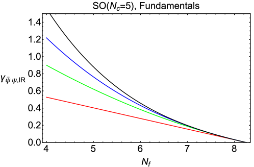
Figure 1: Plot of $\gamma_{\bar{\psi}\psi,IR,F,\Delta_{f}^{p}}$ (labelled as $\gamma_{\bar{\psi}\psi,IR}$ on the vertical axis) for an SO(5) gauge theory with fermions in the fundamental representation $R=F$, with $1\leq p\leq 4$, as a function of $N_{f}\in I$. From bottom to top, the curves (with colors online) refer to $\gamma_{\bar{\psi}\psi,IR,F,\Delta_{f}}$ (red), $\gamma_{\bar{\psi}\psi,IR,F,\Delta_{f}^{2}}$ (green), $\gamma_{\bar{\psi}\psi,IR,F,\Delta_{f}^{3}}$ (blue), and $\gamma_{\bar{\psi}\psi,IR,F,\Delta_{f}^{4}}$ (black).

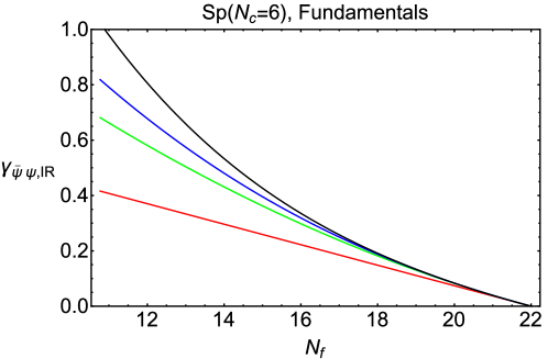
Figure 2: Plot of $\gamma_{\bar{\psi}\psi,IR,F,\Delta_{f}^{p}}$ (labelled as $\gamma_{\bar{\psi}\psi,IR}$ on the vertical axis) for an Sp(6) gauge theory with fermions in the fundamental representation, $R=F$, with $1\leq p\leq 4$, as a function of $N_{f}\in I$. From bottom to top, the curves (with colors online) refer to $\gamma_{\bar{\psi}\psi,IR,F,\Delta_{f}}$ (red), $\gamma_{\bar{\psi}\psi,IR,F,\Delta_{f}^{2}}$ (green), $\gamma_{\bar{\psi}\psi,IR,F,\Delta_{f}^{3}}$ (blue), and $\gamma_{\bar{\psi}\psi,IR,F,\Delta_{f}^{4}}$ (black).

Similarly, as an explicit example of our calculations of $\gamma_{\bar{\psi}\psi,IR}$ to $O(\Delta_{f}^{p})$ with $1\leq p\leq 4$ for an Sp($N_{c}$) group, we will consider an Sp(6) gauge group, again with fermions in the fundamental representation. We choose this example rather than Sp(4) because of the isomorphism ${\rm SO}(5)\cong{\rm Sp}(4)$ (see Appendix A.) From Eqs. (9) and (11) we obtain the values $N_{u,F}=22$ and $N_{\ell}=1088/101=10.772$ nfintegral , so that, with $N_{f}$ generalized to real numbers, the interval $I$ is $10.772<N_{f}<22$ of which the physical, integral values of $N_{f}$ are given by the interval $11\leq N_{f}\leq 21$. In Fig. 2 we present a plot of our $O(\Delta_{f}^{p})$ scheme-independent calculations of $\gamma_{\bar{\psi}\psi,F,IR}$, viz., $\gamma_{\bar{\psi}\psi,IR,F,\Delta_{f}^{p}}$, with $1\leq p\leq 4$. Applying our monotonicity conjecture and estimation methods in the same way as with the SO(5) example above, we are led to the inference that $N_{f,cr}$ is somewhat below the lower end of the interval $I$. As was the case with SO(5), we are not aware of any lattice study of this theory with which we could compare these inferences.

It is straightforward to use our calculations for $\kappa_{j}$ in Eqs. (54)-(65) to compute $\gamma_{\bar{\psi}\psi,IR,F,\Delta_{f}^{p}}$ with $1\leq p\leq 4$ for SO($N_{c}$) and Sp($N_{c}$) theories with $R=F$ and other values of $N_{c}$, and to make estimates of the lower end of the NACP for these other $N_{c}$, but the examples given above should suffice to illustrate the method.

We next mention some checks on our general calculation of the $\kappa_{j}$ coefficients for SO($N_{c}$) and Sp($N_{c}$) with $R=F$. One has the isomorphism ${\rm SO}(3)\cong{\rm SU}(2)$, and, as part of this, the fundamental representation of SO(3) is equivalent to the adjoint representation of SU(2). Hence,

$$\kappa_{j,F,{\rm SO}(3)}=\kappa_{j,A,{\rm SU}(2)}\quad\forall\ j\ ,$$ (66)

where we have indicated the gauge group $G$ and the fermion representation $R$ as subscripts. Using our previous calculations of $\kappa_{j}$ for the SU($N_{c}$) gauge theory with fermions in the adjoint representation, we have verified that our present calculation of $\kappa_{j}$ satisfies this check. Explicitly, with the different gauge groups indicated explicitly, we have

$$\kappa_{1,F,{\rm SO}(3)}=\kappa_{1,A,{\rm SU}(2)}=\frac{2^{2}}{3^{2}}=0.444444\ ,$$ (67)

$$\kappa_{2,F,{\rm SO}(3)}=\kappa_{2,A,{\rm SU}(2)}=\frac{341}{2\cdot 3^{6}}=0.233882\ ,$$ (68)

$$\kappa_{3,F,{\rm SO}(3)}=\kappa_{3,A,{\rm SU}(2)}=\frac{51217}{2^{3}\cdot 3^{10}}=0.108421\ ,$$ (69)

and

$$\kappa_{4,F,{\rm SO}(3)}=\kappa_{4,A,{\rm SU}(2)}=\frac{47764753}{2^{7}\cdot 3^{14}}+\frac{9592}{3^{11}}\zeta_{3}=0.143107\ .$$ (70)

From the explicit expressions above, we calculate the following values of the $\hat{\kappa}_{j,F}$, which are the same in the LNN limits of the SO($N_{c}$) and Sp($N_{c}$) theories (with the numerical values given to the indicated precision):

$$\hat{\kappa}_{1,F}=\frac{2^{3}}{5^{2}}=0.320000\ ,$$ (71)

$$\hat{\kappa}_{2,F}=\frac{2^{4}\cdot 147}{5^{6}}=0.150528\ ,$$ (72)

$$\hat{\kappa}_{3,F}=\frac{2^{6}\cdot 274243}{3^{3}\cdot 5^{10}}=0.0665659\ ,$$ (73)

and

$$\hat{\kappa}_{4,F} = \frac{2^{11}\cdot 1645909}{3^{4}\cdot 5^{13}}+\frac{2^{17}\cdot 11}{3^{3}\cdot 5^{10}}\,\zeta_{3}+\frac{2^{14}\cdot 11}{3^{3}\cdot 5^{8}}\,\zeta_{5}$$ (74)

$$= 0.0583830\ .$$ (76)

Here we have indicated the simple factorizations of the denominators. In general, the numerators do not have simple factorizations, although they often contain various powers of 2, as indicated. We shall generally use this factorization format throughout the paper.

III.2 $R=A$

For $R=A$, we find the following coefficients, where again the upper and lower signs refer to SO($N_{c}$) and Sp($N_{c}$). The floating-point values are quoted to the indicated numerical precision:

$$\kappa_{1,A}=\Big{(}\frac{2}{3}\Big{)}^{2}=0.444444\ ,$$ (77)

$$\kappa_{2,A}=\frac{341}{2\cdot 3^{6}}=0.233882\ ,$$ (78)

$$\kappa_{3,A}=\frac{61873N_{c}^{3}\mp 360582N_{c}^{2}+593292N_{c}\mp 153992}{2^{3}\cdot 3^{10}(N_{c}\mp 2)^{3}}\ ,$$ (79)

and

$$\kappa_{4,A} = \frac{1}{2^{7}\cdot 3^{14}(N_{c}\mp 2)^{3}}\,\bigg{[}\Big{(}53389393N_{c}^{3}\mp 314711718N_{c}^{2}+561927756N_{c}\mp 247126664\Big{)}$$ (82)

$$+\Big{(}3815424N_{c}^{3}\mp 52227072N_{c}^{2}+456468480N_{c}\mp 969228288\Big{)}\zeta_{3}\ \bigg{]}\ .$$

For our two specific illustrative theories, SO(5) and Sp(6), the interval $I$ is the same and is given by Eq. (36). In Figs. 3 and 4 we show plots of $\gamma_{\bar{\psi}\psi,IR,\Delta_{f}^{p}}$ with $1\leq p\leq 4$ for this adjoint case $R=A$, as a function of $N_{f}$ formally generalized to a real variable. The curves are rather similar, as a consequence of the fact that $\kappa_{1,A}$ and $\kappa_{2,A}$ are the same and are independent of $N_{c}$, and, furthermore, the differences between $\kappa_{j,A,{\rm SO}(5)}$ and $\kappa_{j,A,{\rm Sp}(6)}$ are small for $j=3,4$. As we found in our SU($N_{c}$) studies gtr ; dex ; dexs ; dexl , the convergence of the $\Delta_{f}$ expansion is slightly slower for $R=A$ than $R=F$, and this also tends to be true for the other rank-2 tensor representations. We find that, for both SO(5) and Sp(6), as $N_{f}$, formally generalized to a real number, decreases in the interval $I$, $\gamma_{\bar{\psi}\psi,IR}$ calculated to its highest order, $O(\Delta_{f}^{4})$, exceeds the conformality upper bound of 2 as $N_{f}$ reaches about $N_{f}\simeq 1.3$, before it decreases all the say to the lower end of this interval, at $N_{f}=1.0625$. This reduction in the non-Abelian Coulomb phase (conformal window), relative to the full interval $I$ that we find here is similar to what was observed for SU($N$) theories with higher representations in rs_conformalwindow .

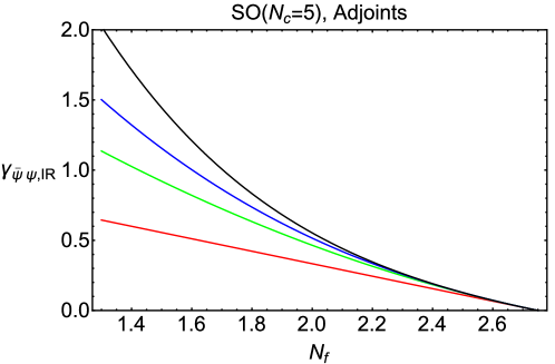
Figure 3: Plot of $\gamma_{\bar{\psi}\psi,IR,A,\Delta_{f}^{p}}$ (labelled as $\gamma_{\bar{\psi}\psi,IR}$ on the vertical axis) for an SO(5) gauge theory with fermions in the adjoint representation $R=A$, with $1\leq p\leq 4$, as a function of $N_{f}\in I$. From bottom to top, the curves (with colors online) refer to $\gamma_{\bar{\psi}\psi,IR,A,\Delta_{f}}$ (red), $\gamma_{\bar{\psi}\psi,IR,A,\Delta_{f}^{2}}$ (green), $\gamma_{\bar{\psi}\psi,IR,A,\Delta_{f}^{3}}$ (blue), and $\gamma_{\bar{\psi}\psi,IR,A,\Delta_{f}^{4}}$ (black).

Figure 4: Plot of $\gamma_{\bar{\psi}\psi,IR,A,\Delta_{f}^{p}}$ (labelled as $\gamma_{\bar{\psi}\psi,IR}$ on the vertical axis) for an Sp(6) gauge theory with fermions in the adjoint representation $R=A$, with $1\leq p\leq 4$, as a function of $N_{f}\in I$. From bottom to top, the curves (with colors online) refer to $\gamma_{\bar{\psi}\psi,IR,A,\Delta_{f}}$ (red), $\gamma_{\bar{\psi}\psi,IR,A,\Delta_{f}^{2}}$ (green), $\gamma_{\bar{\psi}\psi,IR,A,\Delta_{f}^{3}}$ (blue), and $\gamma_{\bar{\psi}\psi,IR,A,\Delta_{f}^{4}}$ (black).

In addition to the manifestly positive $\kappa_{1,A}$ and $\kappa_{2,A}$, we find, by numerical evaluation, that $\kappa_{3,A}$ and $\kappa_{4,A}$ are positive for all relevant $N_{c}$ for both types of gauge groups.

Since the Lie algebras of SU(4) and SO(6) are isomorphic, it follows that

$$\kappa_{j,A,{\rm SO}(6)}=\kappa_{j,A,{\rm SU}(4)}\ .$$ (83)

This requirement serves as another check on our calculations. The check is obviously satisfied for $\kappa_{1,A}$ and $\kappa_{2,A}$. Further, we obtain

$$\kappa_{3,A,{\rm SO}(6)}=\kappa_{3,A,{\rm SU}(4)}=\frac{59209}{2^{3}\cdot 3^{10}}=0.125339$$ (84)

and

$$\kappa_{4,A,{\rm SO}(6)} = \kappa_{4,A,{\rm SU}(4)}$$ (85)

$$= \frac{51983233}{2^{7}\cdot 3^{14}}+\frac{3226}{3^{11}}\zeta_{3}=0.106800$$ (87)

In the LN limit, $\lim_{LN}\kappa_{j,A}$ is the same for SO($N_{c}$) and Sp($N_{c}$). The coefficients $\kappa_{1,A}$ and $\kappa_{2,A}$ are evidently independent of $N_{c}$. The values of $\kappa_{3,A}$ and $\kappa_{4,A}$ in the LN limit are (with numerical values given to the indicated precision)

$$\lim_{N_{c}\to\infty}\kappa_{3,A}=\frac{61873}{2^{3}\cdot 3^{10}}=0.1309871$$ (90)

and

$$\lim_{N_{c}\to\infty}\kappa_{4,A}=\frac{53389393}{2^{7}\cdot 3^{14}}+\frac{368}{3^{10}}\zeta_{3}=0.0946976\ .$$ (91)

III.3 $R=S_{2}$ in SO($N_{c}$) and $R=A_{2}$ in Sp($N_{c}$)

It is convenient to give results for $R=S_{2}$ in SO($N_{c}$) and $R=A_{2}$ in Sp($N_{c}$) together, since they are simply related by sign reversals in certain terms. Recall that for SO($N_{c}$), $N_{c}$ must be $\geq 5$ if $R=S_{2}$ in order for the theory to be asymptotically free. In the following expressions, the upper sign refers to $R=S_{2}$ in SO($N_{c}$) and the lower sign to $R=A_{2}$ in Sp($N_{c}$). We will use a compact notation in which $T_{2}$ refers to these two respective cases. From our general formulas we calculate

$$\kappa_{1,T_{2}}=\frac{4N_{c}(N_{c}\pm 2)}{(N_{c}\mp 2)(9N_{c}\mp 7)}\ ,$$ (92)

$$\kappa_{2,T_{2}}=\frac{N_{c}(N_{c}\pm 2)^{2}(11N_{c}\mp 14)(93N_{c}\mp 10)}{6(N_{c}\mp 2)^{2}(9N_{c}\mp 7)^{3}}\ ,$$ (93)

$$\kappa_{3,T_{2}} = \frac{N_{c}(N_{c}\pm 2)^{2}}{2^{3}\cdot 3^{3}(N_{c}\mp 2)^{3}(9N_{c}\mp 7)^{5}}\bigg{[}\Big{(}1670571N_{c}^{5}\mp 1075194N_{c}^{4}-7188904N_{c}^{3}\pm 14840368N_{c}^{2}$$ (96)

$$+2671344N_{c}\mp 6795040\Big{)}\pm 2^{10}\cdot 33(9N_{c}\mp 7)(3N_{c}^{3}\pm 23N_{c}^{2}-38N_{c}\mp 56)\zeta_{3}\bigg{]}\ ,$$

and

$$\kappa_{4,T_{2}} = \frac{N_{c}(N_{c}\pm 2)^{3}}{2^{7}\cdot 3^{4}(N_{c}\mp 2)^{4}(9N_{c}\mp 7)^{7}}\,\bigg{[}\Big{(}4324540833N_{c}^{7}\mp 6239517858N_{c}^{6}-9953927772N_{c}^{5}\pm 61550306040N_{c}^{4}$$ (103)

$$-90479597392N_{c}^{3}\mp 24158962016N_{c}^{2}+61198146240N_{c}\mp 11095638400\Big{)}$$

$$+2^{10}(9N_{c}\mp 7)\Big{(}33534N_{c}^{6}\pm 743769N_{c}^{5}+4721805N_{c}^{4}\mp 16060070N_{c}^{3}-5795540N_{c}^{2}\pm 16964328N_{c}+3786048\Big{)}\zeta_{3}$$

$$\mp 2^{14}\cdot 275(N_{c}\mp 2)(9N_{c}\mp 7)^{2}(15N_{c}^{3}\pm 139N_{c}^{2}+234N_{c}\pm 120)\zeta_{5}\ \bigg{]}\ .$$

We next apply these results for our two specific illustrative theories, SO(5) and Sp(6). In the SO(5) theory with $R=S_{2}$, $N_{u,{\rm SO}(5),S_{2}}=33/28=1.1786$ and $N_{\ell,{\rm SO}(5),S_{2}}=51/140=0.3643$, while in the Sp(6) theory with $R=A_{2}$, $N_{u,{\rm Sp}(6),S_{2}}=5.5$ and $N_{\ell,{\rm Sp}(6),S_{2}}=68/29=2.345$. In Figs. 5 and 6 we show plots of $\gamma_{\bar{\psi}\psi,IR,R,\Delta_{f}^{p}}$ with $1\leq p\leq 4$ for SO(5) with $R=S_{2}$ and for Sp(6) with $R=A_{2}$, respectively, with $N_{f}$ formally generalized to a real number. We see that in the SO(5) theory, as $N_{f}$ decreases in the interval $I$, $\gamma_{\bar{\psi}\psi,S_{2},IR}$ calculated to its highest order, $O(\Delta_{f}^{4})$, exceeds the conformality upper bound $N_{f}\leq 2$ reaches about $N_{f}\simeq 0.7$, well above the lower end of $I$ at 0.3643. In the Sp(6) theory, as $N_{f}$ decreases in the interval $I$, $\gamma_{\bar{\psi}\psi,A_{2},IR}$ calculated to its highest order, $O(\Delta_{f}^{4})$, exceeds the conformality upper bound $N_{f}\leq 2$ reaches about $N_{f}\simeq 2.4$, close to the lower end of $I$ at 2.345.

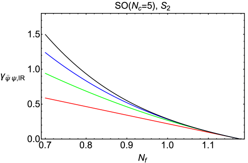
Figure 5: Plot of $\gamma_{\bar{\psi}\psi,IR,S_{2},\Delta_{f}^{p}}$ (labelled as $\gamma_{\bar{\psi}\psi,IR}$ on the vertical axis) for an SO(5) gauge theory with fermions in the $S_{2}$ representation, with $1\leq p\leq 4$, as a function of $N_{f}\in I$. From bottom to top, the curves (with colors online) refer to $\gamma_{\bar{\psi}\psi,IR,S_{2},\Delta_{f}}$ (red), $\gamma_{\bar{\psi}\psi,IR,S_{2},\Delta_{f}^{2}}$ (green), $\gamma_{\bar{\psi}\psi,IR,S_{2},\Delta_{f}^{3}}$ (blue), and $\gamma_{\bar{\psi}\psi,IR,S_{2},\Delta_{f}^{4}}$ (black).

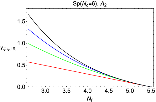
Figure 6: Plot of $\gamma_{\bar{\psi}\psi,IR,A_{2},\Delta_{f}^{p}}$ (labelled as $\gamma_{\bar{\psi}\psi,IR}$ on the vertical axis) for an Sp(6) gauge theory with fermions in the $A_{2}$ representation, with $1\leq p\leq 4$, as a function of $N_{f}\in I$. From bottom to top, the curves (with colors online) refer to $\gamma_{\bar{\psi}\psi,IR,A_{2},\Delta_{f}}$ (red), $\gamma_{\bar{\psi}\psi,IR,A_{2},\Delta_{f}^{2}}$ (green), $\gamma_{\bar{\psi}\psi,IR,A_{2},\Delta_{f}^{3}}$ (blue), and $\gamma_{\bar{\psi}\psi,IR,A_{2},\Delta_{f}^{4}}$ (black).

In addition to the manifestly positive $\kappa_{1,T_{2}}$ and $\kappa_{2,T_{2}}$, we find, by numerical evaluation, that $\kappa_{3,T_{2}}$ and $\kappa_{4,T_{2}}$ are positive for all relevant $N_{c}$ in these SO($N_{c}$) and Sp($N_{c}$) theories.

These coefficients have the same LN limits as the $\kappa_{j,A}$

$$\lim_{N_{c}\to\infty}\kappa_{j,T_{2}}=\lim_{N_{c}\to\infty}\kappa_{j,A}\ .$$ (104)

IV Calculation of $\beta^{\prime}_{IR}$ to $O(\Delta_{f}^{5})$ Order

IV.1 $R=F$

For the coefficients $d_{j}$, we recall first that $d_{1}=0$ for all $G$ and $R$. As was true of the $\kappa_{j,R}$ coefficients, the $d_{j,R}$ coefficients for SO($N_{c}$) and Sp($N_{c}$) are simply related to each other with sign reversals in various terms, and hence it is natural to present them together. Concerning the signs of these coefficients, our general expressions in dex for $d_{2}$ and $d_{3}$ show that they are positive for arbitrary $G$ and $R$:

$$d_{2}=\frac{2^{5}T_{f}^{2}}{3^{2}C_{A}(7C_{A}+11C_{f})}\ ,$$ (105)

and

$$d_{3}=\frac{2^{7}T_{f}^{3}(5C_{A}+3C_{f})}{3^{3}C_{A}^{2}(7C_{A}+11C_{f})^{2}}\ .$$ (106)

Since our general expressions for $d_{4}$ in dex and for $d_{5}$ in dexs ; dexl contain negative terms, it is necessary to investigate the signs of these terms as a function of $G$, $R$, and $N_{c}$.

For the fundamental representation, we obtain the following results, where, as before, the upper and lower signs refer to SO($N_{c}$) and Sp($N_{c}$), respectively:

$$d_{2,F}=\frac{2^{6}}{3^{2}(N_{c}\mp 2)(25N_{c}\mp 39)}\ ,$$ (107)

$$d_{3,F}=\frac{2^{8}(13N_{c}\mp 23)}{3^{3}(N_{c}\mp 2)^{2}(25N_{c}\mp 39)^{2}}\ ,$$ (108)

$$d_{4,F} = \frac{2^{8}}{3^{5}(N_{c}\mp 2)^{3}(25N_{c}\mp 39)^{5}}\,\bigg{[}\Big{(}366782N_{c}^{4}\mp 2269256N_{c}^{3}+5506308N_{c}^{2}\mp 6383412N_{c}+2994975\Big{)}$$ (111)

$$-2^{5}\cdot 33(N_{c}\mp 3)(25N_{c}\mp 39)(25N_{c}^{2}\mp 65N_{c}+94\Big{)}\zeta_{3}\ \bigg{]}\ ,$$

and

$$d_{5,F} = \frac{2^{10}}{3^{6}(N_{c}\mp 2)^{4}(25N_{c}\mp 39)^{7}}\,\bigg{[}\Big{(}-298194551N_{c}^{6}\pm 3084573642N_{c}^{5}-13173836397N_{c}^{4}$$ (118)

$$\pm 29649471936N_{c}^{3}-37042033788N_{c}^{2}\pm 24377774904N_{c}-6624643320\Big{)}$$

$$-2^{5}(25N_{c}\mp 39)(529125N_{c}^{5}\mp 4349794N_{c}^{4}+14556219N_{c}^{3}\mp 23420126N_{c}^{2}+15005784N_{c}\mp 467496\Big{)}\zeta_{3}$$

$$+2^{7}\cdot 55(N_{c}\mp 2)(N_{c}\mp 3)(25N_{c}\mp 39)^{2}(120N_{c}^{2}\mp 229N_{c}+511)\zeta_{5}\ \bigg{]}\ .$$

In addition to the manifestly positive $d_{2}$ and $d_{3}$, for SO($N_{c}$), we find that $d_{4,F}$ is positive if $N_{c}=3$, but decreases through zero and is negative for large $N_{c}$, while $d_{5,F}$ is negative for the relevant range $N_{c}$. For Sp($N_{c}$), we find that both $d_{4,F}$ and $d_{5,F}$ are negative in the relevant range of (even) $N_{c}$.

As $N_{c}\to\infty$, the $d_{j,F}\propto 1/N_{c}^{j}+O(1/N_{c}^{j+1})$, and hence the finite coefficients for the scheme-independent expansion of $\beta^{\prime}_{IR}$ in this limit are

$$\hat{d}_{j,F}=\lim_{N_{c}\to\infty}N_{c}^{j}d_{j,F}\ .$$ (119)

These limiting values are the same for SO($N_{c}$) and Sp($N_{c}$). From our results above, we calculate

$$\hat{d}_{2,F}=\frac{2^{6}}{3^{2}\cdot 5^{2}}=0.284444\ ,$$ (120)

$$\hat{d}_{3,F}=\frac{2^{8}\cdot 13}{3^{3}\cdot 5^{4}}=0.197215\ ,$$ (121)

$$\hat{d}_{4,F} = \frac{2^{9}\cdot 183391}{3^{5}\cdot 5^{10}}-\frac{2^{13}\cdot 11}{3^{4}\cdot 5^{6}}\zeta_{3}$$ (122)

$$= -0.0460182\ ,$$ (124)

and

$$\hat{d}_{5,F} = -\frac{2^{10}\cdot 298194551}{3^{6}\cdot 5^{14}}-\frac{2^{15}\cdot 1411}{3^{5}\cdot 5^{9}}\zeta_{3}+\frac{2^{20}\cdot 11}{3^{5}\cdot 5^{8}}\zeta_{5}$$ (125)

$$= -0.0597277\ .$$ (127)

IV.2 $R=A$

As discussed above, for the SO($N_{c}$) and Sp($N_{c}$) theories with $R=A$, the adjoint representation, only one value of $N_{f}$ is allowed by asymptotic freedom and lies in the interval $I$, namely $N_{f}=2$. We calculate the following results for the $d_{j,A}$, with $N_{c}$ kept in as a formal variable (and with numerical values given to the indicated precision)

$$d_{2,A}=\Big{(}\frac{2}{3}\Big{)}^{4}=0.197531\ ,$$ (128)

$$d_{3,A}=\frac{2^{8}}{3^{7}}=0.117055\ ,$$ (129)

$$d_{4,A} = \frac{1}{2^{2}\cdot 3^{12}(N_{c}\mp 2)^{3}}\,\Big{(}46871N_{c}^{3}\mp 302538N_{c}^{2}+860820N_{c}\mp 1056952\Big{)}\ ,$$ (130)

and

$$d_{5,A} = \frac{1}{2^{3}\cdot 3^{16}(N_{c}\mp 2)^{3}}\,\bigg{[}\Big{(}-7141205N_{c}^{3}\pm 43403934N_{c}^{2}-93488316N_{c}\pm 74944168\Big{)}$$ (133)

$$+\Big{(}3566592N_{c}^{3}\pm 3718656N_{c}^{2}-308855808N_{c}\pm 775249920\Big{)}\zeta_{3}\bigg{]}\ .$$

The $N_{c}\to\infty$ limits of $d_{j,A}$ are the same for SO($N_{c}$) and Sp($N_{c}$). We have

$$\lim_{N_{c}\to\infty}d_{4,A}=\frac{46871}{2^{2}\cdot 3^{12}}=2.204901\times 10^{-2}$$ (134)

and

$$\lim_{N_{c}\to\infty}d_{5,A} = -\frac{7141205}{2^{3}\cdot 3^{16}}+\frac{2^{7}\cdot 43}{3^{12}}\zeta_{3}$$ (135)

$$= -(0.8287386\times 10^{-2})\ .$$ (137)

In addition to the manifestly positive $d_{2,A}$ and $d_{3,A}$, we find that for SO($N_{c}$), in the relevant range of $N_{c}$, $d_{4,A}$ is positive, while $d_{5,A}$ is negative. For Sp($N_{c}$), $d_{4,A}$ is manifestly positive, and we find that $d_{5,A}$ is negative.

IV.3 $R=S_{2}$ in SO($N_{c}$) and $R=A_{2}$ in Sp($N_{c}$)

As before, we present our results for $R=S_{2}$ in SO($N_{c}$) and $R=A_{2}$ in Sp($N_{c}$) together, since they are simply related by sign reversals in certain terms. Recall that for SO($N_{c}$), $N_{c}$ must be $\geq 5$ if $R=S_{2}$ in order for the theory to be asymptotically free. In the following expressions, the upper sign refers to $R=S_{2}$ in SO($N_{c}$) and the lower sign to $R=A_{2}$ in Sp($N_{c}$). We again use the compact notation in which $T_{2}$ refers to these two respective cases. From our general formulas we calculate

$$d_{2,T_{2}}=\frac{2^{4}(N_{c}\pm 2)^{2}}{3^{2}(N_{c}\mp 2)(9N_{c}\mp 7)}\ ,$$ (138)

$$d_{3,T_{2}}=\frac{2^{6}(N_{c}\pm 2)^{3}(4N_{c}\mp 5)}{3^{3}(N_{c}\mp 2)^{2}(9N_{c}\mp 7)^{2}}\ ,$$ (139)

$$d_{4,T_{2}} = \frac{(N_{c}\pm 2)^{3}}{2^{2}\cdot 3^{5}(N_{c}\mp 2)^{3}(9N_{c}\mp 7)^{5}}\,\bigg{[}\Big{(}1265517N_{c}^{5}\mp 618894N_{c}^{4}+3021512N_{c}^{3}\mp 10811760N_{c}^{2}$$ (142)

$$-16432368N_{c}\pm 16806048\Big{)}\pm 2^{12}\cdot 33(9N_{c}\mp 7)(3N_{c}^{3}\mp 15N_{c}^{2}+N_{c}\pm 42)\zeta_{3}\ \bigg{]}\ ,$$

and

$$d_{5,T_{2}} = \frac{(N_{c}\pm 2)^{4}}{2^{3}\cdot 3^{6}(N_{c}\mp 2)^{4}(9N_{c}\mp 7)^{7}}\,\bigg{[}\Big{(}-578437605N_{c}^{7}\pm 3437217450N_{c}^{6}-6404128380N_{c}^{5}\mp 13828926056N_{c}^{4}$$ (149)

$$+52499838288N_{c}^{3}\mp 21845334432N_{c}^{2}-14381806656N_{c}\pm 6247244416\Big{)}$$

$$+2^{9}(9N_{c}\mp 7)\Big{(}62694N_{c}^{6}\pm 61965N_{c}^{5}-6430023N_{c}^{4}\pm 11443586N_{c}^{3}+10920884N_{c}^{2}\mp 16105176N_{c}-1862112\Big{)}\zeta_{3}$$

$$\mp 2^{13}\cdot 55(N_{c}\mp 2)(N_{c}\mp 9)(9N_{c}\mp 7)^{2}(87N_{c}^{2}\pm 178N_{c}+48)\zeta_{5}\ \bigg{]}\ .$$

Concerning signs, in addition to the manifestly positive $d_{2,T_{2}}$ and $d_{3,T_{2}}$, we find that for SO($N_{c}$) with $N_{c}\geq 5$, $d_{4,S_{2}}>0$ and $d_{5,S_{2}}<0$, while for Sp($N_{c}$), $d_{4,A_{2}}<0$ if $N_{c}=4$, $d_{4,A_{2}}>0$ if $N_{c}\geq 6$, and $d_{5,A_{2}}<0$ for all $N_{c}\geq 4$. We further note that

$$\lim_{N_{c}\to\infty}d_{j,T_{2}}=\lim_{N_{c}\to\infty}d_{j,A}\ .$$ (150)

V Conclusions

In this paper we have used our general calculations in gtr ; gsi ; dex ; dexl to obtain scheme-independent results for the anomalous dimension, $\gamma_{\bar{\psi}\psi,IR}$, and the derivative of the beta function, $\beta^{\prime}_{IR}$, at an infrared fixed point of the renormalization group in the non-Abelian Coulomb phase of vectorial, asymptotically free SO($N_{c}$) and (with even $N_{c}$) Sp($N_{c}$) gauge theories with fermions in several different irreducible representations, namely fundamental, adjoint, and rank-2 symmetric and antisymmetric tensor. We calculate $\gamma_{\bar{\psi}\psi,IR}$ to $O(\Delta_{f}^{4})$ and $\beta^{\prime}_{IR}$ to $O(\Delta_{f}^{5})$, where $\Delta_{f}$ is the expansion parameter defined in Eq. (1). These are the highest orders to which these quantities have been calculated for these theories. Our present results extend our earlier ones for the case of SU($N_{c}$) gauge theories in gtr ; gsi ; dex ; dexs ; dexl to these other two types of gauge groups.

An important question that we address and answer is whether the coefficients $\kappa_{j}$ in the expansion (2) are positive for SO($N_{c}$) and Sp($N_{c}$) with all of the representations that we consider, just as we found earlier for SU($N_{c}$). We find that the answer is affirmative. Our finding yields two monotonicity results for these SO($N_{c}$) and Sp($N_{c}$) groups and representations, namely that (i) $\gamma_{\bar{\psi}\psi,IR,\Delta_{f}^{p}}$ increases monotonically as $N_{f}$ decreases from $N_{u}$ in the non-Abelian Coulomb phase; (ii) for a fixed $N_{f}$ in the NACP, $\gamma_{\bar{\psi}\psi,IR,\Delta_{f}^{p}}$ increases monotonically with $p$. Our results in this paper provide further support for our conjecture that, in addition to the manifestly positive $\kappa_{1}$ and $\kappa_{2}$, the $\kappa_{j}$ for $j\geq 3$ are positive for a vectorial asymptotically free gauge theory with a general (simple) gauge group $G$ and fermion representations $R$ that we have considered. In turn, this conjecture implies several monotonicity properties, namely the generalizations of (i) and (ii) to arbitrary $p$ and thus the property that the quantity $\gamma_{\bar{\psi}\psi,IR}$ defined by the infinite series (2), increases monotonically with decreasing $N_{f}$ in the non-Abelian Coulomb phase. Using this property in conjunction with the upper bound on $\gamma_{\bar{\psi}\psi,IR}$ in a conformally invariant theory, and the assumption that this bound is saturated at the lower end of the NACP (as it is in the exact results for an ${\cal N}=1$ supersymmetric gauge theory), we have given estimates of the lower end of this non-Abelian Coulomb phase for illustrative theories of these types.

Appendix A Some Group-Theoretic Quantities

In this appendix we discuss some group-theoretic quantities that enter in our calculations. As in the text, we denote the gauge group as $G$. The generators of the Lie algebra of this group, in the representation $R$, are denoted $T^{a}_{R}$, with $1\leq a\leq d_{A}$. The generators satisfy the Lie algebra

$$[T^{a}_{R},T^{b}_{R}]=if^{abc}T^{c}_{R}\ ,$$ (151)

where the $f^{abc}$ are the associated structure constants of this Lie algebra. Here and elsewhere a sum over repeated indices is understood. We denote the dimension of a given representation $R$ as $d_{R}={\rm dim}(R)$. In particular, as in the text, we denote the adjoint representation by $A$, with the dimension $d_{A}$ equal to the number of generators of the group, i.e., the order of the group. (The dimension $d_{A}$ should not be confused with the tensors $d_{A}^{abcd}$.) The normalization of the generators is given by the trace in the representation $R$,

$${\rm Tr}_{R}(T^{a}_{R}T^{b}_{R})=T(R)\delta_{ab}\ .$$ (152)

The quadratic Casimir invariant $C_{2}(R)$ is given by

$$T^{a}_{R}T^{a}_{R}=C_{2}(R)I\ ,$$ (153)

where $I$ is the $d_{R}\times d_{R}$ identity matrix. For a fermion $f$ transforming according to a representation $R$, we often use the equivalent compact notation $T_{f}\equiv T(R)$ and $C_{f}\equiv C_{2}(R)$. We also use the notation $C_{A}\equiv C_{2}(A)\equiv C_{2}(G)$. The invariants $T(R)$ and $C_{2}(R)$ are related according to

$$C_{2}(R)d_{R}=T(R)d_{A}\ .$$ (154)

A remark on the normalization of the generators is in order. As was noted in b4 ; invariants , although the normalization $T(F)=1/2$, where $F$ is the fundamental representation, is standard for the trace in Eq. (152) for SU($N$), two normalizations are widely used for this normalization for SO($N$) and Sp($N$) groups. As indicated, our normalization is $T(F)=1$ for SO($N$) and $T(F)=1/2$ for Sp($N$). If one multiplies $T(R)$ by a factor $\rho$, this is equivalent to multiplying the generators and structure constants by $\sqrt{\rho}$ and the quadratic Casimir invariant $C_{2}(R)$ by $\rho$. In the covariant derivative $D_{\mu}=\partial_{\mu}\cdot 1-g{\vec{T}}\cdot{\vec{A}}_{\mu}$, where $A^{a}_{\mu}$ is the gauge field, a rescaling of the generators by $\sqrt{\rho}$ means that $g$ is rescaling by $1/\sqrt{\rho}$, with the gauge field continuing to have canonical normalization. Physical quantities such as $N_{u}$, $N_{\ell}$, $\gamma_{\bar{\psi}\psi,IR}$, and $\beta^{\prime}_{IR}$ are independent of this normalization convention with $\rho$. This can be seen from Eqs. (9), (11), and the explicit expressions that we have given in our earlier works gtr ; gsi ; dex ; dexs ; dexl for the coefficients $\kappa_{j}$ and $d_{j}$. For example, in the expressions $\kappa_{2}=8C_{f}T_{f}/[C_{A}(7C_{A}+11C_{f})]$ and $d_{2}=32T_{f}^{2}/[9C_{A}(7C_{A}+11C_{f})]$, both the numerator and denominator scale like $\rho^{2}$, so this normalization factor cancels, and similarly for other $\kappa_{j}$ and $d_{j}$.

In this appendix we will, for generality, consider the three types of gauge groups SU($N$), SO($N$), and Sp($N$). As noted before, the correspondence between the mathematical notation for the Cartan series of Lie algebras and our notation used here is $A_{n}={\rm SU}(n+1)$, $B_{n}={\rm SO}(2n+1)$, $C_{n}={\rm Sp}(2n)$, and $D_{n}=SO(2n)$. One may recall some basic properties of these Lie groups and their associated Lie algebras (see, e.g., grouptheoryrefs -patera ). Concerning representations, SU(2) has only real representations, while SU($N$) with $N\geq 3$ has complex representations. Sp($N$) ($N$ even) and SO($N$) with odd $N$ have only real representations, while SO($N$) with even $N$ also have both real and complex representations. Concerning the values of $N_{f}$, we note that for a real representation, one could consider half-integral $N_{f}$, corresponding to a Majorana fermion. However, this would entail a global Witten anomaly associated with the homotopy group $\pi_{4}(G)$ in the case $G={\rm SO}(N)$ with $N=3,\ 4,\ 5$, and for all Sp($N$) (while $\pi_{4}({\rm SO}(N))=\emptyset$ for $N\geq 6$ finkelstein .) Hence, we restrict to integer $N_{f}$, i.e., Dirac fermions.

In Tables 1 we list the dimensions and quadratic group invariants for SU($N$), SO($N$), and Sp($N$) groups with the various representations considered in the text patera . The results for SU($N$) are well-known, but some remarks are in order for SO($N$) and Sp($N$). An element $O$ of SO($N$) satisfies $OO^{T}=1$. Starting with a 2-index tensor $\psi=\psi^{ij}$ of SO($N$), we can form symmetric and antisymmetric quantities in the obvious way by taking sums and differences of $\psi$ and $\psi^{T}$. However, to form the irreducible symmetric representation of SO($N$), $S_{2}$, it is necessary to remove the trace, so we write

$$\psi = \frac{1}{2}(\psi+\psi^{T})-{\rm Tr}(\psi)\cdot 1$$ (155)

$$+ \frac{1}{2}(\psi-\psi^{T})$$ (157)

$$+ {\rm Tr}(\psi)\cdot 1\ ,$$ (159)

where here $1$ is the $N\times N$ identity matrix. The quantities in the first and second lines of Eq. (159) form the (traceless) $S_{2}$ and $A_{2}$ representations of SO($N$) (the latter being automatically traceless), while the quantity in the third line is a singlet. The dimensions of the $S_{2}$ and $A_{2}$ representations are therefore

$$d_{S_{2},{\rm SO}(N)}=\frac{N(N+1)}{2}-1=\frac{(N-1)(N+2)}{2}$$ (160)

and $d_{A_{2},{\rm SO}(N)}=N(N-1)/2=d_{A,{\rm SO}(N)}$, as listed in the table.

An element $S$ of Sp($N$) satisfies $SES^{T}=E$, with $E$ the antisymmetric $N\times N$ matrix

$$E=\left(\begin{array}[]{cc}0&1\\ -1&0\end{array}\right)\ ,$$ (161)

where here the symbols $0$ and $1$ denote $N/2\times N/2$ submatrices. We can thus write

$$\psi = \frac{1}{2}(\psi+\psi^{T})$$ (162)

$$+ \frac{1}{2}(\psi-\psi^{T})-{\rm Tr}(\psi)E$$ (164)

$$+ {\rm Tr}(\psi)E\ ,$$ (166)

The quantities in the first and second lines of Eq. (166) form the $S_{2}$ and $A_{2}$ representations of Sp($N$), while the third line is a singlet. The dimensions of the $S_{2}$ and $A_{2}$ representations are therefore $d_{S_{2},{\rm Sp}(N)}=N(N+1)/2=d_{A,{\rm Sp}(N)}$, and

$$d_{A_{2},{\rm Sp}(N)}=\frac{N(N-1)}{2}-1=\frac{(N+1)(N-2)}{2}\ ,$$ (167)

as listed in the table. We remark that the expressions for $T(R)$ and $C_{2}(R)$ for Sp($N$) are simply related to those for SO($N$) by a factor of 1/2 and sign reversals of certain terms.

At the four-loop and five-loop level, new types of group-theoretic invariants appear in the coefficients for the beta function and anomalous dimension $\gamma_{\bar{\psi}\psi,IR}$, namely the four-index quantities $d^{abcd}_{R}$. For a given representation $R$ of $G$,

$$d^{abcd}_{R} = \frac{1}{3!}{\rm Tr}_{R}\Big{[}T_{a}(T_{b}T_{c}T_{d}+T_{b}T_{d}T_{c}+T_{c}T_{b}T_{d}$$ (168)

$$+ T_{c}T_{d}T_{b}+T_{d}T_{b}T_{c}+T_{d}T_{c}T_{b})\Big{]}\ .$$ (170)

From Eq. (170), it is evident that $d^{abcd}_{R}$ is a totally symmetric function of the group indices $a,b,c,d$. One can express this as

$$d_{R}^{abcd} = I_{4,R}d^{abcd}+\Big{(}\frac{T(R)}{d_{A}+2}\Big{)}\Big{(}C_{2}(R)-\frac{1}{6}C_{A}\Big{)}\times$$ (171)

$$\times (\delta^{ab}\delta^{cd}+\delta^{ac}\delta^{bd}+\delta^{ad}\delta^{bc})\ ,$$ (173)

where $d^{abcd}$ is traceless (i.e., $\delta_{ab}d^{abcd}=0$, etc.), $I_{4,R}$ is a quartic group invariant (index) okubo ; patera , and $d_{A}$ is the dimension of the adjoint representation, i.e., the number of generators of the Lie algebra of $G$. The traceless tensor $d^{abcd}$ depends only on the group $G$, but not on the representation $R$. The quartic indices $I_{4,R}$ are listed for the relevant representations in Table 2. The quantities that appear in the coefficients that we calculate involve products of these $d_{R}^{abcd}$ of the form $d_{R}^{abcd}d_{R^{\prime}}^{abcd}$, summed over the group indices $a,\ b,\ c,\ d$. These can be written as

$$d^{abcd}_{R}d^{abcd}_{R^{\prime}}=I_{4,R}I_{4,R^{\prime}}d^{abcd}d^{abcd}+$$ (174)

(175)

$$+\Big{(}\frac{3d_{A}}{d_{A}+2}\Big{)}T(R)T(R^{\prime})\Big{(}C_{R}-\frac{1}{6}C_{A}\Big{)}\Big{(}C_{R^{\prime}}-\frac{1}{6}C_{A}\Big{)}\ .$$ (176)

(177)

(178)

One has, for the quartic Casimir invariants that depend only on $G$, the results b4 ; invariants

$${\rm SU}(N):\quad d^{abcd}d^{abcd}=\frac{d_{A}(d_{A}-3)(d_{A}-8)}{96(d_{A}+2)}\ ,$$ (179)

$${\rm SO}(N):\quad d^{abcd}d^{abcd}=\frac{d_{A}(d_{A}-1)(d_{A}-3)}{12(d_{A}+2)}\ ,$$ (180)

and

$${\rm Sp}(N):\quad d^{abcd}d^{abcd}=\frac{d_{A}(d_{A}-1)(d_{A}-3)}{192(d_{A}+2)}\ ,$$ (181)

so that $d^{abcd}d^{abcd}$ for Sp($N$) is formally 1/16 times the corresponding quantity for SO($N$) (with different $d_{A}$ understood). Note that $d^{abcd}d^{abcd}=0$ for SU(2), SO(3), and Sp(2), since the dimension of the adjoint representation in all three cases is $d_{A}=3$. This is in agreement with the isomorphisms ${\rm SU}(2)\cong{\rm Sp}(2)$ and ${\rm SU}(2)\cong{\rm SO}(3)$. (These may be considered to refer to the Lie algebras; for our purposes, we do not have to distinguish between local and global isomorphisms.) Note also that $d^{abcd}d^{abcd}=0$ for SU(3), since $d_{A}=8$ for SU(3).

We list the resultant values of $d_{R}^{abcd}d_{R^{\prime}}^{abcd}$ in Tables 3. As is evident from these tables, the expressions for the $d_{R}^{abcd}d_{R^{\prime}}^{abcd}$ for Sp($N$) are simply related to those for SO($N$) by an overall factor of $1/16$ and sign reversals of certain coefficients. Our results for SU($N$) agree with the corresponding entries in Table II in ps ; however, our results for $d^{abcd}_{R}d^{abcd}_{R}$ and $d^{abcd}_{R}d^{abcd}_{A}$ differ from those given in Table II of ps for SO($N$) and Sp($N$) comm . We have performed several checks on the correctness of our results:

1. Since ${\rm SU}(4)\cong{\rm SO}(6)$, the coefficients $\kappa_{j},\ j=1,\dots,4$ and $d_{j},\ j=1\dots,5$ calculated for ${\rm SU}(4)$ must agree with their counterparts for SO(6) when the matter representations are equivalent. We have checked that this is satisfied in a number of cases. Specifically, this must hold for (i) the 20-dimensional $S_{2}$ representation of SO(6) and the real 20-dimensional representation of $SU(6)$ with Dynkin label (0,2,0); (ii) the fundamental 6-dimensional representation of SO(6) and the 6-dimensional $A_{2}$ representation of SU(4); and (iii) the adjoint representation of both SU(4) and SO(6). The group invariants for the real 20-dimensional representation of SU(4) with Dynkin label (0,2,0) we have used are $T_{f}=8$ and $C_{f}=6$ perelman_popov .

2. Since the adjoint representation of SU(2) is equivalent to the adjoint as well as the fundamental representation of SO(3), it follows that the corresponding coefficients $\kappa_{j},\ j=1,\dots,4$ and $d_{j},\ j=1\dots,5$ should be equal, and we have verified that this is the case.

3. Since ${\rm SU}(2)\cong{\rm Sp}(2)$, it follows that the expressions for $\kappa_{j}$ and $d_{j}$ should be the same for our representations $R$ for these two groups, and they are.

4. The isomorphism SO(5) $\cong$ Sp(4) pss yields a further check on our results. The invariants for the adjoint representations of these groups must be equal and they are. Further, the fundamental representation of SO(5) has the same dimension as the $A_{2}$ representation of Sp(4), and these yield the same $\kappa_{j}$ and $d_{j}$ values, which provides a check on our expressions for the $A_{2}$ representation of Sp($N$).

Table 1: Values of various group invariants for the groups SU($N$), SO($N$), and (with even $N$) Sp($N$) and (irreducible) fermion representations $R$ equal to fundamental ($F$), adjoint ($A$), and rank-2 symmetric ($S_{2}$) and antisymmetric ($A_{2}$) tensor. We take $N\geq 2$ for SU($N$), $N\geq 3$ for SO($N$), and even $N\geq 2$ for Sp($N$). Here, $d_{R}$ denotes the dimension of the representation $R$. For a fermion $f$ in the representation $R$, the equivalent compact notation $T_{f}\equiv T(R)$ and $C_{f}\equiv C_{2}(R)$ is used in the text.

${\rm SU}(N),\ N\geq 2$
$R$	$d_{R}$	$T(R)$	$C_{2}(R)$
$F$	$N$	$\frac{1}{2}$	$\frac{N^{2}-1}{2N}$
$A$	$N^{2}-1$	$N$	$N$
$S_{2}$	$\frac{N(N+1)}{2}$	$\frac{N+2}{2}$	$\frac{(N-1)(N+2)}{N}$
$A_{2}$	$\frac{N(N-1)}{2}$	$\frac{N-2}{2}$	$\frac{(N+1)(N-2)}{N}$

${\rm SO}(N),\ N\geq 3$
$R$	$d_{R}$	$T(R)$	$C_{2}(R)$
$F$	$N$	$1$	$\frac{N-1}{2}$
$A$	$\frac{N(N-1)}{2}$	$N-2$	$N-2$
$S_{2}$	$\frac{(N-1)(N+2)}{2}$	$N+2$	$N$

${\rm Sp}(N),\ N\geq 2$
$R$	$d_{R}$	$T(R)$	$C_{2}(R)$
$F$	$N$	$\frac{1}{2}$	$\frac{N+1}{4}$
$A$	$\frac{N(N+1)}{2}$	$\frac{N+2}{2}$	$\frac{N+2}{2}$
$A_{2}$	$\frac{(N+1)(N-2)}{2}$	$\frac{N-2}{2}$	$\frac{N}{2}$

Table 2: Values of $I_{4,f}$ indices for the groups SU($N$), SO($N$), and (with even $N$), Sp($N$) and and fermion representations $R$ equal to fundamental ($F$), adjoint ($A$), and rank-2 symmetric ($S_{2}$) and antisymmetric ($A_{2}$) tensor. $S_{2}$ (symmetric rank-2 tensor).

$I_{4,f}$	SU$(N)$	SO$(N)$	Sp$(N)$
$F$	$1$	$1$	$1$
$A$	$2N$	$N-8$	$N+8$
$S_{2}$	$N+8$	$N+8$	$N+8$
$A_{2}$	$N-8$	$N-8$	$N-8$

Table 3: Values of $d_{R}^{abcd}d_{R^{\prime}}^{abcd}/d_{A}$ for groups SU($N$), SO($N$), and Sp($N$) and irreducible representations $R$ equal to fundamental ($F$), adjoint ($A$), and rank-2 symmetric ($S_{2}$) and antisymmetric ($A_{2}$) tensors.

${\rm SU}(N),\ N\geq 2$
$R$	$d_{R}^{abcd}d_{R}^{abcd}/d_{A}$	$d_{R}^{abcd}d_{A}^{abcd}/d_{A}$
$F$	$\frac{N^{4}-6N^{2}+18}{96N^{2}}$	$\frac{N(N^{2}+6)}{48}$
$A$	$\frac{N^{2}(N^{2}+36)}{24}$	$\frac{N^{2}(N^{2}+36)}{24}$
$S_{2}$	$\frac{(N+2)(N^{5}+14N^{4}+72N^{3}-48N^{2}-288N+576)}{96N^{2}}$	$\frac{N(N+2)(N^{2}+6N+24)}{48}$
$A_{2}$	$\frac{(N-2)(N^{5}-14N^{4}+72N^{3}+48N^{2}-288N-576)}{96N^{2}}$	$\frac{N(N-2)(N^{2}-6N+24)}{48}$

${\rm SO}(N),\ N\geq 3$
$R$	$d_{R}^{abcd}d_{R}^{abcd}/d_{A}$	$d_{R}^{abcd}d_{A}^{abcd}/d_{A}$
$F$	$\frac{N^{2}-N+4}{24}$	$\frac{(N-2)(N^{2}-7N+22)}{24}$
$A$	$\frac{(N-2)(N^{3}-15N^{2}+138N-296)}{24}$	$\frac{(N-2)(N^{3}-15N^{2}+138N-296)}{24}$
$S_{2}$	$\frac{(N+2)(N^{3}+13N^{2}+110N+104)}{24}$	$\frac{(N-2)(N+2)(N^{2}-N+28)}{24}$

${\rm Sp}(N),\ N\geq 2$
$R$	$d_{R}^{abcd}d_{R}^{abcd}/d_{A}$	$d_{R}^{abcd}d_{A}^{abcd}/d_{A}$
$F$	$\frac{N^{2}+N+4}{384}$	$\frac{(N+2)(N^{2}+7N+22)}{384}$
$A$	$\frac{(N+2)(N^{3}+15N^{2}+138N+296)}{384}$	$\frac{(N+2)(N^{3}+15N^{2}+138N+296)}{384}$
$A_{2}$	$\frac{(N-2)(N^{3}-13N^{2}+110N-104)}{384}$	$\frac{(N+2)(N-2)(N^{2}+N+28)}{384}$

References

- (1) Since our gauge theories are vectorial, fermion mass terms are allowed by gauge invariance, but a fermion with nonzero mass would be integrated out of the low-energy effective field theory that describes the physics at Euclidean momentum scales and hence would not affect the infrared limit that we consider here. Note that we also exclude scalar fields.
- (2) D. J. Gross and F. Wilczek, Phys. Rev. Lett. 30, 1343 (1973); H. D. Politzer, Phys. Rev. Lett. 30, 1346 (1973); G. ’t Hooft, unpublished.
- (3) W. E. Caswell, Phys. Rev. Lett. 33, 244 (1974); D. R. T. Jones, Nucl. Phys. B 75, 531 (1974).
- (4) Our analysis is based on being an exact IR fixed point (IRFP) of the renormalization group. We remark that for sufficiently smaller values of , the gauge interaction produces spontaneous chiral symmetry breaking and associated dynamical fermion mass generation at some scale . The now-massive fermions are then integrated out of the effective field theory that is applicable for scales , thereby changing the beta function to that of a pure gauge theory. Hence, evolves away from , which is thus only an approximate, but not exact, IRFP.
- (5) Some early analyses of relations between scale and conformal invariance are A. Salam, Ann. Phys. (NY) 53, 174 (1969); A. M. Polyakov, JETP Lett. 12, 381 (1970); D. J. Gross and J. Wess, Phys. Rev. D 2, 753 (1970); C. G. Callan, S. Coleman, and R. Jackiw, Ann. Phys. (NY) 59, 42 (1970). More recent papers include J. Polchinski, Nucl. Phys. B 303, 226 (1988); J.-F. Fortin, B. Grinstein and A. Stergiou, JHEP 01 (2013) 184 (2013); A. Dymarsky, Z. Komargodski, A. Schwimmer, and S. Thiessen, JHEP 10, 171 (2015) and references therein.
- (6) D. J. Gross, in R. Balian and J. Zinn-Justin, eds. Methods in Field Theory, Les Houches 1975 (North Holland, Amsterdam, 1976), p. 141.
- (7) T. Banks and A. Zaks, Nucl. Phys. B 196, 189 (1982).
- (8) E. Gardi and M. Karliner, Nucl. Phys. B 529, 383 (1998); E. Gardi and G. Grunberg, JHEP 03, 024 (1999).
- (9) T. A. Ryttov, Phys. Rev. Lett. 117, 071601 (2016).
- (10) T. A. Ryttov and R. Shrock, Phys. Rev. D 94, 105014 (2016).
- (11) T. A. Ryttov and R. Shrock, Phys. Rev. D 94 125005 (2016).
- (12) T. A. Ryttov and R. Shrock, Phys. Rev. D 95, 085012 (2017)
- (13) T. A. Ryttov and R. Shrock, Phys. Rev. D 95, 105004 (2017)
- (14) J. A. Gracey, Phys. Lett. B 488, 175 (2000).
- (15) In contrast, from our explicit calculations in dex , we also found that this uniform positivity does not hold for the coefficients in the expansion of in powers of or in the coefficients of the power series for the anomalous dimension of the Dirac tensor fermion bilinear , where is the antisymmetric Dirac tensor.
- (16) F. Sannino, Phys. Rev. D 79, 096007 (2009); F. Sannino, Acta Phys. Polonica B 40, 3533 (2009).
- (17) M. Mojaza, C. Pica, T. A. Ryttov, and F. Sannino, Phys. Rev. D 86, 076012 (2012).
- (18) G. Mack, Commun. Math. Phys. 55, 1 (1977); B. Grinstein, K. Intriligator, and I. Rothstein, Phys. Lett. B 662, 367 (2008); Y. Nakayama, Phys. Repts. 569, 1 (2015).
- (19) Parenthetically, we note that a different appoach to study the onset of spontaneous chiral symmetry breaking (SSB) is via a solution, in the ladder approximation, of the Schwinger-Dyson equation for the fermion propagator. This leads to SSB as : K. Yamawaki, M. Bando, and K. Matumoto, Phys. Rev. Lett. 56, 1335 (1986); T. Appelquist, D. Karabali, and L. C. R. Wijewardhana, Phys. Rev. Lett. 57, 957 (1986).
- (20) N. Seiberg, Nucl. Phys. B435, 129 (1995).
- (21) K. A. Intriligator and N. Seiberg, Nucl. Phys. (Proc. Suppl.) 45BC, 1 (1996); M. A. Shifman, Prog. Part. Nucl. Phys. 39, 1 (1997); J. Terning, Modern Supersymmetry (Clarendon Press, Oxford, 2006).
- (22) Here and elsewhere, when an expression is given for that formally evaluates to a non-integral real value, it is understood implicitly that one infers an appropriate integral value from it.
- (23) T. A. Ryttov and R. Shrock, arXiv:1706.06422.
- (24) Some comparisons of exact and perturbative results in supersymmetric gauge theories were made in T. A. Ryttov and R. Shrock, Phys. Rev. D 85, 076009 (2012); A. L. Kataev and K. V. Stepanyantz, Phys. Lett. B 730, 184 (2014); Theor. Math. Phys. 181, 1531 (2014); R. Shrock, Phys. Rev. D 91, 125039 (2015); G. Choi and R. Shrock, Phys. Rev. D 93, 065013 (2016).
- (25) O. V. Tarasov, A. A. Vladimirov, and A. Yu. Zharkov, Phys. Lett. B 93, 429 (1980); S. A. Larin and J. A. M. Vermaseren, Phys. Lett. B 303, 334 (1993).
- (26) K. G. Chetyrkin, Phys. Lett. B 404, 161 (1997); T. van Ritbergen, J. A. M. Vermaseren, and S. A. Larin, Phys. Lett. B 400, 379 (1997).
- (27) P. A. Baikov, K. G. Chetyrkin, and J. H. Kühn, Phys. Rev. Lett. 118, 082002 (2017).
- (28) F. Herzog, B. Ruijl, T. Ueda, J. A. M. Vermaseren, and A. Vogt, JHEP 02 (2017) 090.
- (29) W. A. Bardeen, A. J. Buras, D. W. Duke, and T. Muta, Phys. Rev. D 18, 3998 (1978).
- (30) J. A. M. Vermaseren, S. A. Larin, and T. van Ritbergen, Phys. Lett. B 405, 327 (1997).
- (31) P. A. Baikov, K. G. Chetyrkin, and J. H. Kuhn, JHEP 1704, 119 (2017).
- (32) T. A. Ryttov, R. Shrock, Phys. Rev. D 83, 056011 (2011).
- (33) C. Pica, F. Sannino, Phys. Rev. D 83, 035013 (2011).
- (34) R. Shrock, Phys. Rev. D 87, 105005 (2013); R. Shrock, Phys. Rev. D 87, 116007 (2013).
- (35) T. A. Ryttov and R. Shrock, Phys. Rev. D 94, 105015 (2016).
- (36) T. A. Ryttov and R. Shrock, Phys. Rev. D 86, 065032 (2012); T. A. Ryttov and R. Shrock, Phys. Rev. D 86, 085005 (2012); R. Shrock, Phys. Rev. D 88, 036003 (2013); R. Shrock, Phys. Rev. D 90, 045011 (2014); R. Shrock, Phys. Rev. D 91, 125039 (2015); G. Choi and R. Shrock, Phys. Rev. D 90, 125029 (2014); G. Choi and R. Shrock, Phys. Rev. D 94, 065038 (2016).
- (37) T. A. Ryttov, Phys. Rev. D 89, 016013 (2014); T. A. Ryttov, Phys. Rev. D 89, 056001 (2014); T. A. Ryttov, Phys. Rev. D 90, 056007 (2014).
- (38) J. A. Gracey and R. M. Simms, Phys. Rev. D 91, 085037 (2015).
- (39) Some authors use the opposite sign convention for the anomalous dimension, writing .
- (40) S. S. Gubser, A. Nellore, S. S. Pufu, and E. D. Rocha, Phys. Rev. Lett. 101, 131601 (2008).
- (41) T. A. Ryttov and F. Sannino, Phys. Rev. D 76, 105004 (2007).
- (42) T. van Ritbergen, A. N. Schellekens, and J. A. M. Vermaseren, Int. J. Mod. Phys. A 14, 41 (1999).
- (43) See, e.g., R. Slansky, Phys. Rept. 79, 1 (1981); H. Georgi, Lie Algebras in Particle Physics, 2nd ed. (Perseus, Reading MA, 1999) W.-K. Tung, Group Theory in Physics (World Scientific, Philadelphia, 1985).
- (44) A. M. Pereleman and V. S. Popov, Sov. J. Nucl. Phys. 3, 676, 819 (1966); 7, 290 (1968); E. Eichten and F. Feinberg, Phys. Lett. B 110, 232 (1982).
- (45) S. Okubo, J. Math. Phys. 23, 8 (1982); S. Okubo and J. Patera, J. Math. Phys. 25, 219 (1984).
- (46) J. Patera, R. T. Sharp, and P. Winternitz, J. Math. Phys. 17, 1972 (1976).
- (47) D. Finkelstein and J. Rubinstein, J. Math Phys. 9, 1762 (1968) and references therein.
- (48) D. D. Dietrich and F. Sannino, Phys. Rev. D 75, 085018 (2007).
- (49) J. Patera, R. Sharp, and R. Slansky, J. Math. Phys. 21, 2335 (1980).
- (50) We thank C. Pica and F. Sannino, for discussions on in Ref. ps and M. Mojaza on mps .
- (51) M. Mojaza, C. Pica, and F. Sannino, Phys. Rev. D 82, 116009 (2010) (Note the different normalization of generators.)