[options= -s indexstyle.ist]

Urban Delay Tolerant Network Simulator
(UDTNSim v0.1)

Abstract

Delay Tolerant Networking (DTN) is an approach to networking which handles network disruptions and high delays that may occur in many kinds of communication networks. The major reasons for high delay include partial connectivity of networks as can be seen in many types of ad-hoc wireless networks with frequent network partitions, long propagation time as experienced in inter-planetary and deep space networks, and frequent link disruptions due to the mobility of nodes as observed in terrestrial wireless network environments. Experimenting network architectures, protocols, and mobility models in such real-world scenarios is difficult due to the complexities involved in the network environment. Therefore, in this document, we present the documentation of an Urban Delay Tolerant Network Simulator (UDTNSim) version 0.1, capable of simulating urban road network environments with DTN characteristics including mobility models and routing protocols. The mobility models included in this version of UDTNSim are (i) Stationary Movement, (ii) Simple Random Movement, (iii) Path Type Based Movememt, (iv) Path Memory Based Movement, (v) Path Type with Restricted Movement, and (vi) Path Type with Wait Movement. In addition to mobility models, we also provide three routing and data hand-off protocols: (i) Epidemic Routing, (ii) Superior Only Handoff, and (iii) Superior Peer Handoff. UDTNSim v0.1 is designed using object-oriented programming approach in order to provide flexibility in addition of new features to the DTN environment. UDTNSim v0.1 is distributed as an open source simulator for the use of the research community.

Contents

1. Abstract
2. 1 Introduction
3. 2 UDTNSim Architecture
   1. 2.1 A Modular View of UDTNSim
   2. 2.2 Implementation of Modules
   3. 2.3 Simulator Configuration
      1. 2.3.1 Simulation Parameters
      2. 2.3.2 Parser
      3. 2.3.3 Addition of New Simulation Parameters
      4. 2.3.4 XML Parser
   4. 2.4 Summary
4. 3 Movement Models
   1. 3.1 Stationary Movement
   2. 3.2 Simple Random Movement
   3. 3.3 Path Type Based Movement Model
   4. 3.4 Path Memory Based Movement Model
   5. 3.5 Path Type with Restricted Movement
   6. 3.6 Path Type with Wait Movement
   7. 3.7 Addition of New Movement Models
   8. 3.8 Summary
5. 4 Routing Protocols
   1. 4.1 Epidemic Routing
   2. 4.2 Superior Only Handoff Protocol
   3. 4.3 Superior Peer Handoff Protocol
   4. 4.4 Addition of New Routing Protocols
   5. 4.5 Summary
6. 5 Supporting Libraries
   1. 5.1 Graphical User Interface
   2. 5.2 Events
      1. 5.2.1 Event
      2. 5.2.2 Event Operations
   3. 5.3 Reports
      1. 5.3.1 Movement Report
      2. 5.3.2 Event Report
   4. 5.4 Additional Libraries
   5. 5.5 Summary
7. 6 Summary
   1. 6.1 Related Work in UDTNSim
8. Bibliography

List of Figures

1. 2.1 A sample simulation scenario.
2. 2.2 A snapshot of UDTNSim using the map of Dharavi, India.
3. 2.3 UDTN simulator architecture.
4. 2.4 Example view of the settings object
5. 5.1 Snapshot of simulator GUI.

Chapter 1 Introduction

Delay Tolerant Networking (DTN) is the area of networking which can address the challenges in disconnected and disrupted networks without an end-to-end connection [1]. Real world wireless networks experience delays due to several factors such as long transmission time, obstacles in line-of-sight, and disruption of the links resulting from low transmission range and node mobility. Delay due to long transmission time occurs in interplanetary communications, whereas, frequent link-breaks (disruptions) are the major cause of end-to-end delay in mobile ad-hoc networks such as vehicular networks.

An architecture for DTN [1] is proposed with an addition of a bundle layer between the application and transport layer of traditional OSI model. A protocol known as bundle protocol [2] is designed to manage the operations of bundle layer. The layer creates its own data units, known as bundles, from the data it received from the application layer. In case of significant delays, the bundle layer stores the bundles until it gets an opportunity to handover the data to the destination or to a node with a higher chance of delivering the message toward the destination. That is, the bundle layer uses a store-and-forward approach, known as custody-transfer, in transferring the data towards the subsequent nodes. In order to achieve reliability in communication, the node to which the data is transferred takes the responsibility of custodian of the message so that the message can be delivered without loss.

Several routing protocols are developed for efficient communication in DTNs. Some of them include epidemic protocol [3], spray and wait [4], MaxProp [5], and PROPHET [6]. The protocols use different metrics such as delivery probability of nodes, history of nodes’ contacts, the time for delivery, and buffer size for computing the routing decision. In general, the protocols are designed to maximize the delivery probability while minimizing the transmission time, data loss, and communication overhead.

Similar to routing, in case of networks in terrestrial environments such as vehicular networks, mobility pattern of the nodes has significant influence on the network delay. The mobility pattern varies with different networks. Examples of different mobility patterns include mobility of vehicles in a road network, mobility of boats in the sea, and mobility of drones. The quality of routing decisions depends on how accurately we can predict the mobility pattern of nodes and, thereby, the contacts between them. Random mobility makes the task more challenging. Moreover, there occur situations where we need to design mobility pattern if we have sufficient information about the terrain. For example, in a disaster environment, we need to design efficient mobility patterns for the emergency response personnel to respond to emergency calls with available resources. Therefore, mobility models are very important aspect in delay tolerant networks.

Experimenting mobility models and DTN protocols in a real world set-up may not be feasible always. Simulations provide better options for testing and evaluating new mobility models and routing protocols. Here, we discuss an Urban Delay Tolerant Network Simulator (UDTNSim) [7], developed using Python-2.7 [8], which is capable of creating DTN environments with real world node mobility and associated routing protocols. The simulator provides considerable flexibility in adding modules to customize as per our requirements.

Chapter 2 UDTNSim Architecture

The simulation environment is defined using a geographical area with a road network and objects (stationary well as mobile). The stationary objects include sensors, wireless routers, and other devices which provide wireless connectivity to objects. Mobile agents (for example bikes, cars, humans, and drones) connected with wireless devices are represented as mobile objects. Stationary objects can be positioned (either at random or using custom algorithms) in the specified geographical area and mobile nodes move through the area either through roads, in case of vehicles, or through air, in case of drones, and communicate with other mobile nodes as well as stationary nodes. The purpose of network includes data gathering from sensors and communication between different kinds of objects. Figure 2.1 shows an example scenario with a road network and set of stationary and mobile objects.

Figure 2.1: A sample simulation scenario.

In Figure 2.1, highways are represented as black lines and the roads which are accessible for two-wheeler objects as red lines. Yellow triangles represent stationary nodes (sensors) which are distributed in the geographic area. The mobile objects are represented using filled circles (black circle represents four-wheeler vehicles and red, the two-wheeler vehicles). From Figure 2.1, it is clear the four-wheeler vehicles can only access the highways (black lines) and two-wheeler vehicles can access both highways as well as two-wheeler ways (red lines). The mobile nodes can move through the road network and collect data from the stationary nodes. A moving object can communicate with another when they come in the range of each other, i.e., while they are in contact. If the destination node for a message is not in the transmission range, the source can forward the message to an object which has a higher chance of meeting with the destination. A simulation snapshot of UDTNSim using the map of shanty town Dharavi, India, is shown in Figure 2.2. Since the simulation is based on the real world scenario, we use object oriented programming approach for its implementation.

Figure 2.2: A snapshot of UDTNSim using the map of Dharavi, India.

2.1 A Modular View of UDTNSim

The UDTN simulator is divided into eight modules to simplify the process of adding new features or modifying the existing ones. Figure 2.3 shows the architecture of the simulator with different modules and their interactions.

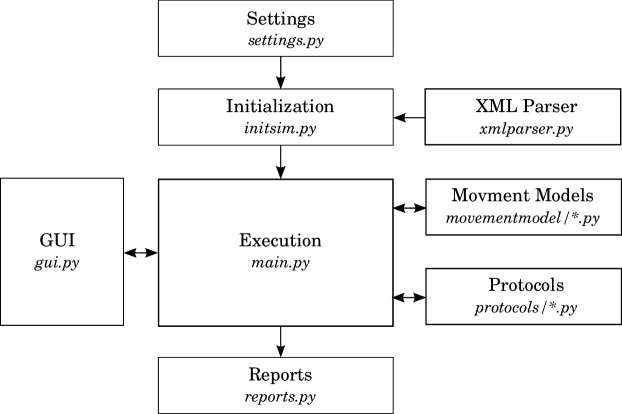
Figure 2.3: UDTN simulator architecture.

1. Settings: Module to provide the simulation environment. It includes a configuration file ‘sim.config’ as well as the libraries to parse the configuration file.

2. XML Parser: Module to parse the geographical location from the map information (which is in XML format extracted from OpenStreetMap[9]) and convert it into simulation variables.

3. Initialization: The module initializes the simulator environment using the configuration provided by the user as well as the map information.

4. Movement Models: Handles different movement models for the objects.

5. Protocols: Defines routing protocols for the objects.

6. Execution: Coordinates different modules and execute the simulation. Execution module communicates with Movement Models, Protocols, GUI, and Reports modules.

7. GUI: Handles the graphical user interface of the simulator.

8. Reports: Creates of simulation-related logs.

2.2 Implementation of Modules

Each component of the simulator is implemented using objected oriented programming approach to make the code reusable and provide flexibility. For example, the basis of movement model module is a class to represent stationary objects with basic attributes such as a unique ID, its geographical position, and a buffer to store data. The concept of mobility is introduced from stationary object with the addition of functions required for the position change, i.e., the mobility. In other words, the class for a mobile object can be defined by inheriting properties from the stationary object. In similar way, different kinds of mobility can be defined from the mobility class with redefinition of the function for position change. Therefore, object oriented programming approach provide the developers more flexibility in adding new features with minimum effort.

2.3 Simulator Configuration

For any simulator, the execution environment is specified in terms of simulation parameters. As we discussed at the beginning of this chapter, the simulator consists of a geographical area and objects (both stationary and mobile). We need to specify the parameters required for each of these components. For example, the geographical area is specified as a map (represented using XML). The map can be exported from www.openstreetmap.org[9], in .osm format. The parameters for a mobile object include ID, the road-types it can travel, buffer size, mobility model, and routing protocol.

In general, the parameters are specified using a configuration file. We use a file sim.config to specify the environmental parameters (such as simulation name, simulation time, map information, and report directory) and the movement object specific parameters (such as group label, transmission range, buffer size, and speed).

2.3.1 Simulation Parameters

Simulation parameters are classified into two: (i) general parameters and (ii) node specific parameters.

2.3.1.1 General Parameters

General parameters include those which are required for every component in the simulator.

1. Simulation_Name: Provides a name for the simulation.

2. No_of_Simulations: In most cases, especially in cases where randomness is involved, we need to run the simulations multiple times and aggregate the observations obtained from each of them. The parameter No_of_Simulations allows to set the required number of simulations.

3. Simulation_Time: Represents the real world simulation time specified in hours.

4. Map: Represents the map of geographical area in .osm format. The file should be specified using its path, either absolute or relative. By default, the simulator has a directory maps, where .osm files for different geographical areas can be placed.

5. Report_Directory: Represents the location for placing the simulation logs. The directory can be specified using an absolute or relative path. At present, the simulator has a directory logs for simulation-related logs. In the current version, separate sub-directories are created for each of the objects (See Section 5.3).

6. GUI_Enabled: Enables the Graphical User Interface (GUI). It has two values, True or False. GUI can be enabled for testing the movement models and protocols. Since GUI consumes more CPU time for simulation, it is recommended to make GUI_Enabled = False for simulations which take significant time.

7. Path_Types: Since the simulation environment has a geographical area, we need to specify the types of roads that we consider for our simulation. The mobile objects move through the specified types of roads and communicate with other objects. We need to assign unique numbers for each of the road-types so that the numbers can be used to specify the allowed road-types for each object.

8. Random_Msg_Gen_Parameter: Represents the event generation parameter. Its value is a tuple of the form $[m,n]$, i.e., $m$ events are generated in every $n$ hours.

9. No_of_Hosts_Groups: Indicates the number of object groups present in the simulation. If we have more than one object with same specifications, we can organize them as an host-group. Further, we need to describe the specifications for each group.

2.3.1.2 Group Specific Parameters

Here, we describe the parameters specific for each object group. Every object in a group are assigned with the same parameters specified for that group.

1. Group_ID:Unique ID for the group.

2. Label: Label for distinguishing each group in the simulation GUI. If Label = T, the objects in the group are assigned with names T1, T2, T3, and so on.

3. Paths: Assign the road-types through which the objects in a group can travel. We need to give the list of numbers corresponding to the path-types given in the parameter Path_Types, specified in Section 2.3.1.1.

4. No_of_Hosts: The number of nodes present in the group.

5. TX_Range: Transmission range of the node specified in meters.

6. Buffer_Size: Size of the buffer in each node specified in Kilobytes (K), Megabytes (M), or Gigabytes (G). At present the buffer size is of infinite size.

7. Speed:Speed of the node in kilometer per hour (km/hr).

8. Mobile: Parameter that distinguishes a mobile node from a stationary node. It takes the value either True or False. True represents a mobile node while False, a stationary node.

9. Movement: Represents the mobility model for the nodes. Different movement models such as StationaryMovement, SimpleRandomMovement, and PathTypeMovement are defined in the directory movementmodel.

10. Junction_Delay: Delay that occurred at the road junctions specified in seconds.

11. Color: Color of the nodes in GUI.

12. Protocol: Specifies the routing protocol for the nodes. For example, a node following EpidemicHandoff transfers its data to the nodes which comes in contact with it. In case of SuperiorOnlyHandoff, a node transfers its data only to a node which is higher at the classification hierarchy. A node which acts as Depot do not transfer the data to other nodes, however, it only receives the data from other nodes. The protocols are defined in the subdirectory protocols.

2.3.2 Parser

The code for parsing the configuration file sim.config is written in parser/settings.py. Since the first step of simulation is to read the environment settings, an object of type Settings is created at the start of simulation (in initsim/init.py).

⬇

envt_params = settings.Settings(’sim.config’)

The class Settings contains two dictionaries, envt and groups, which represent general parameters and group specific parameters, respectively. The dictionary envt has the parameter name as the key and the value as the value given by the user. For groups, key is the Group_ID and value as another dictionary with key as parameter name and value the corresponding node specific value. The function read_settings() reads the entire content from the settings file, sim.config, and populate the dictionaries envt as well as groups. Logical view of a Settings object is shown in Figure 2.4.

Attribute	Value
settings_file	‘sim.config’
envt	{‘Simulation_Name’:‘SampleDTN’, ‘GUI_Enabled’:False, …}
groups	{‘G1’:{‘Label’:‘T’, ‘Mobile’:True, …}, ‘G2’:{…}, …}

Figure 2.4: Example view of the settings object

2.3.3 Addition of New Simulation Parameters

As the simulation needs change, there may be a requirement for new set of parameters for the environment as well as for the nodes. Therefore, the simulator provides a provision to add new parameters using two files envt_params.in and group_params.in in the subdirectory parser. For the addition of a new parameter, we need to append a line of the form ParameterName:Type to the file envt_params.in for a general parameter, or to group_params.in for a group specific parameter. If the value corresponding to a parameter is a list with items which are of non-string type, we may need to convert it into appropriate type in the code (either in settings.py or wherever we access that parameter).

2.3.4 XML Parser

We consider the map input as an XML file, in .osm format, exported from openstreetmap.org [9]. In order to extract the information required for the simulation, we define three functions in parser/xmlparser.py file.

1. parse_osm(): This function extracts the map information given in .osm file into two dictionaries, node_dict and way_dict. node_dict keeps the information of geographical points with their latitude, longitude, corresponding cartesian coordinates for GUI, and the identifiers of the roads in which the geographical point takes part in.

   ⬇

   node_dict = {node_id: [(lat, lon), (y, x), [w1, w2, ...], ...}

   Similar to node_dict, way_dict stores the information related to ways (roads). The key is the road identifier and value is a list with node IDs (keys from node_dict) of the geographical points which create the way, the type of the road, and the length of the road (in kilometers).

   ⬇

   way_dict = {way_id: [[node_id1, node_id2,...], way_type, way_length], ...}

   The function takes inputs the osm file and the dimension (height and width) of the simulator GUI. The function is called from init_sim_envt() in init/initsim.py. The map file is taken from the path provided in sim.config using Map parameter.

   ⬇

   Map = maps/manhattan.osm

2. traverse_way(): The XML file extracted from from OpenStreetMap consists of two tags for representing roads (i) <node> and (ii) <way>. The node information (i.e.,the geographical points) from <node> tag is read by the function parse_osm(). We define the function traverse_way() to extract way information given in <way> tags. The function is invoked from the parse_osm() function when it interprets a line with a <way> tag.

   ⬇

   # Detected a ‘way’ tag. The function ‘traverse_way’ is

   # called to retrieve the way information

   elif line.find(‘‘<way’’) + 1:

   components = line.split()

   way_id = int(components[1].split(‘‘\"")[1])

   node_order, way_type, file_ptr = traverse_way(file_ptr, node_dict, way_id)

   # Add way information to way_dict

   if way_type:

   way_dict[way_id] = [node_order, way_type]

3. normalize_map(): The XML file from OpenStreetMap provides the way information, including the geographical points that make the way (roads). The information of road intersections, which is a pre-requisite for representing road network as a graph, is not provided with the XML file. Therefore, the function normalize_map() takes node_dict and way_dict as inputs and finds the road intersections. Further, the ways are divided according to the number of intersections and the dictionaries are modified accordingly.

In order to add a parser for a new type of map file, appropriate functions should be defined in the directory parser. The functions should parse the file and generate two dictionaries, node_dict and way_dict, with the same structure as discussed in the beginning of this section.

2.4 Summary

In this chapter, we discussed the architecture of the UDTN simulator, its configuration, and the parser modules for input parameters. The implementation details of the remaining modules are described in the following chapters.

Chapter 3 Movement Models

Movement models define the mobility pattern of the objects. A classical example is random way-point model [10] where, the node randomly chooses a destination and moves toward it. Once reaching the destination, the node again selects a random destination and the process continues.

Since UDTN simulator considers movement of nodes through a road network, we need to consider the characteristics of each road as well as each object while defining the mobility. For instance, road-type and the type of object (vehicle) are important factors while defining the mobility. That is, four-wheeler nodes such as cars and buses can only travel through the road with sufficient width. For example, cars can easily traverse through a highway, not through a two-wheeler road or a footpath. However, a pedestrian can travel through all types of roads.

In our simulator, we define three movement models: (i) Stationary Movement, (ii) Simple Random Movement, (iii) Path Type Based Movememt, (iv) Path Memory Based Movement, (v) Path Type with Restricted Movement, and (vi) Path Type with Wait Movement.

3.1 Stationary Movement

As the name implies, stationary movement is defined as no movement. Stationary movement is defined especially for static nodes such as sensors and fixed wireless routers or access points. The movement model is defined as a class Stationary in the file stationary.py. Also, the purpose of this movement model is to define the characteristics of an object such as identity, group identity, position (geographic position and its corresponding pixel position in the GUI), storage buffer, and a report mechanism for creating logs. The attributes defined for stationary object include the following:

1. obj_id: Unique identifier for the object.

2. group_id: Identifier of the group where the object belongs. More than one movement objects can have the same group identifier.

3. prev_node: Current vertex identifier (a key from node_dict) of the node, i.e., the junction the object recently visited.

4. next_node: The vertex toward which the object is moving. In stationary movement, next_node is the same as the prev_node.

5. curr_geo_pos: The current geographical position of the node. It is a tuple of the form (lat, lon) where lat and lon represent latitude and longitude, respectively.

6. curr_pix_pos: The current pixel position of the object in the GUI. It is also a tuple of the form (y, x).

7. buffer: A list for storing data.

8. report_obj: An object of MovementReport class to create logs related to the object.

9. protocol_obj: An object of the routing protocol. Different routing protocols are discussed in Chapter 4.

The class Stationary has a member function compute_initial_node(), which randomly chooses a vertex in the geographical location to position the stationary object. That is, the vertex chosen is assigned to the prev_node attribute of stationary node. The function compute_initial_node() can be overridden to position nodes at specific positions as required for the simulation.

3.2 Simple Random Movement

Simple random movement is an adoption of random way-point model on to a road network. Here, unlike stationary movement, the object moves from one vertex (road junction) to the adjacent vertex through the road (edge) connecting them. We define simple random movement model as follows: a node at a vertex randomly chooses a vertex from its adjacent vertices (excluding the adjacent vertex that it comes from) and moves toward the selected vertex through the edge connecting those two vertices. If the vertex is an end point of a road, the object returns back to its previous vertex.

Simple random movement is defined as a class SimpleRandomMovement in file simplerandom. py. The movement model inherits all the properties of stationary node from Stationary class. Further, we define the following additional attributes to realize the movement:

1. curr_way: The way id (key from the dictionary way_dict) of a way where the object locates.

2. speed: Speed of the object in km/hr.

3. ways_visited: A list to store the way_ids of the ways the object already visited.

4. time_traveled: The travel time of the object in seconds.

5. mvmt_points: A list to keep the movement points (geographical as well as pixel points) of the way on which the node is moving. For example, if a node moves from vertex A (prev_node) to vertex B (next_node), the geographical points between A and B are computed and stored in mvmt_points. At each time step, the node moves from one point to the next.

6. mvmt_pt_index: An index to the list mvmt_points, which represents the current position of the node.

Apart from the movement specific attributes, we define three functions to handle the movement:

1. update_position(): At each time step, the function update_position(), changes the position of object through the points specified in mvmt_points (geographical positions of a road). If the object reaches the last position in mvmt_points, i.e., end of the current way, the object needs to choose an adjacent vertex at random, which is done using the function compute_next_node(). If the current position is not the end of the curr_way, the node is shifted to the next position in mvmt_points using an increment to mvmt_pt_index.

2. compute_next_node(): The function chooses an adjacent vertex (junction) from neighboring vertices at random. If the vertex is an end vertex, then the function considers the previous vertex as the next vertex. The next way (link) for the node will be the way connecting the current vertex and next chosen vertex.

3. populate_way_points(): After choosing the next link to travel, we need to find the geographical points between the prev_node and next_node. In order to trace the points that make the link, we interpolate the points using the geographical positions available (from .osm file) in the curr_way. The available geographical points can be assessed using the dictionary way_dict[curr_way][0]. The interpolated points are stored in mvmt_points and the index variable mvmt_pt_index is reset to 0. If any junction delay is specified for the object, we append required number of points (same as the last point in mvmt_points) at the end of mvmt_points.

SimpleRandomMovement is the simplest mobility model for the nodes. The model is more suitable if the road network has only a single type of road or the mobile objects are capable of moving through every type of roads. Here, the movement objects do not consider the type of road for their movement. In order to simulate a more realistic model, it is necessary to consider the types of roads as well as the types of movement objects. Path Type Based Movement is suitable direction toward it.

3.3 Path Type Based Movement Model

Simple random movement may not be realistic if we consider a road network with different types of roads and different types of mobile objects. That is, simple random movement does not distinguish between different types of roads as well as different types of mobile nodes. As explained in the example at the beginning of this chapter, we need to consider the type of vehicle and type of roads it can traverse. Therefore, we define a path-type based movement model where each mobile object chooses an adjacent neighbor vertex only if it has a road with sufficient width to travel toward the destination. For example, a four-wheeler chooses a neighboring vertex only if there exists a highway connecting to that vertex. Therefore, path-type based movement model can be considered as simple random movement with constraints on road-type.

The movement model is defined as a class PathTypeMovement in the file path type.py. Since, the mobile node shares all the properties of simple random movement (except the vertex selection procedure), the class PathTypeMovement is defined as a class derived from Simple RandomMovement. Here, we need to redefine the member functions compute_initial _node() and compute_next_node() to override the functions in simple random movement.

1. compute_initial_node(): When a mobile object gets created, it is positioned at a random vertex in the graph. In path-type movement model, we need to randomly select a vertex with roads attached to it having the type that can be traversed by that object. That is, for computing an initial vertex for a four-wheeler, we need to find a vertex with at least one highway attached to it. In this function, first we find the possible road-types (given in the sim.config file) that the node can traverse using the following statement.

   ⬇

   possible_paths = global_params.envt_params.groups\

   [self.group_id][’Paths’]

   Further we choose a vertex at random from the graph and checks any of its neighbor is connected with a road-type given in possible_paths. If none of the edges are with required type, then the process is repeated with another randomly chosen vertex.

2. compute_next_node(): Similar to simple random movement model, when a node reaches a vertex/junction, it collects the neighbor vertices. Among them, the node creates a list of neighbor vertices (possible_nodes) which are connected by any of the road-types given in its possible_types. From possible_nodes, a vertex is chosen at random as the next_node. If the list possible_nodes is empty, next_node is assigned with the prev_node.

3.4 Path Memory Based Movement Model

Path Memory Based Movement Model is a path-type based model which uses the history of nodes’ traversal for taking decision on further movement. The purpose of path-memory model is to avoid the selection of already traversed roads in the map and, thereby, explore maximum possible locations in the geographical area. Here, the function compute_next_node() is redefined to make the movement memory-based. After computing possible_nodes as in path-type movement model, the function discards already traversed ways using the list ways_traversed.

⬇

untraversed_nodes = [] for node in possible_nodes: if

road_graph[self.next_node][node][’way_id’] not in self.ways_visited:

untraversed_nodes.append(node)

if untraversed_nodes: possible_nodes = untraversed_nodes[:]

In case of no untraversed roads connected to a junction, the algorithm chooses the next way using path-type movement model. The class PathMemoryMovement is defined in the file pathmemory.py.

3.5 Path Type with Restricted Movement

Path Type with Restricted Movement is designed for specific type of nodes where the movement needs to be controlled through certain road-types. For the example discussed at the beginning of Chapter 2, two-wheeler nodes are destined to travel through the remote roads to gather information from sensors. Due to the structure of complex road networks, the density of remote roads is higher compared to that of highways. Therefore, there may occur instances that two-wheeler nodes get trapped in remote roads once they enter into such roads, especially if they follow random movement. Such cases reduce the chances for a two-wheeler to meet with four-wheeler nodes, which travel only through the highways. In restricted movement, when a two-wheeler comes to a junction where a highway is connected, its movement get restricted only through the highways until it meets with a four-wheeler to transfer its data. Upon the data transfer, the restriction is withdrawn and two-wheeler is allowed to continue its journey through the remote roads. In other words, the restriction of two-wheeler movement increases the probability of two-wheeler-four-wheeler contact. Similar to Path Memory Movement, Restricted Movement inherits the properties of Path Type Movement and redefines the function compute_next_node() with the addition of path restriction as shown in the following code.

⬇

# Addition of restriction av_nodes = [] # List for storing connected

highways if self.buffer: # If object has data in its buffer for node

in possible_nodes: e_type =

road_graph[self.next_node][node][’e_type’] if e_type == ’highway’:

av_nodes.append(node) if av_nodes: possible_nodes = av_nodes[:] #

End of restriction

In case of junctions which do not have a highway connected to them, the node follows path-type based movement model. The restricted movement is implemented as class RestrictedMovement in the file restricted.py.

3.6 Path Type with Wait Movement

Path Type with Wait is a variation of Path Type with Restricted Movement on the fact that, whenever a node reaches a particular junction, the node stops its movement until the occurrence of a specific event. For example, a two-wheeler comes with data to a junction where a highway is connected, it waits at that junction for a four-wheeler instead of roaming through the highways as the case with restricted movement. Wait movement is implemented as a class WaitMovement, derived from PathTypeMovement, in the file wait.py. An additional attribute wait_flag is defined to control the waiting of a node at the junctions. The function compute_next_node() is redefined with the wait process as follows.

⬇

# Addition of Waiting Process Code av_nodes = [] if self.buffer: for

node in possible_nodes: e_type =

road_graph[self.next_node][node][’e_type’] if e_type == ’highway’:

av_nodes.append(node) if av_nodes: if not self.wait_flag:

self.wait_start = global_params.sim_time self.wait_flag = True

return self.next_node # End of Waiting Process Code

The value of wait_flag becomes True when a two-wheeler reaches a highway junction, i.e., the two-wheeler waits when its wait_flag = True. In our example, when a four-wheeler comes in contact with the two-wheeler, the value of wait_flag turns to False and two-wheeler resumes its journey as per the path type movement model. The value of wait_flag is assigned to True in the routing protocol since the decision depends on the communication between nodes.

3.7 Addition of New Movement Models

Object oriented programming approach used in UDTN Simulator provides an easy way to define custom movement models. The class SimpleRandomMovement provides the basic movement for the objects and PathTypeMovement provides a realistic movement of vehicles through the road network. In order to incorporate a new movement model, say ABCMovement, we need follow 3 steps.

Step 1:

Create a file abc.py in movementmodel/ directory with the definition of movement model as a class. An example skeleton of abc.py is as follows:

⬇

import random

import simplerandom as sr

class ABCMovement(sr.SimpleRandomMovement):

# ABC movement model

## Constructor

def __init__(self, obj_label, group_id, group_params,\ global_params):

sr.SimpleRandomMovement.__init__(self, obj_label, group_id, group_params, global_params)

## Re-definition of initial_node for ABC movement

def compute_initial_node(self, global_params):

# Statement here

return initial_node

## Redefinition of compute_next_node for ABC movement

def compute_next_node(self, global_params):

# Statements here

return next_node

Step 2:

Edit the function create_mvmt_object() in init/initsim.py by adding an elif statement with information of ABCMovement. An example code is given below:

⬇

def create_mvmt_object(obj_label, group_id, group_params, global_params):

obj_type = group_params[’Movement’]

if obj_type == ’Stationary’:

return stationary.Stationary(obj_label,\

group_id, group_params, global_params)

elif obj_type == ’SimpleRandomMovement’:

return simplerandom.SimpleRandomMovement(obj_label, group_id, group_params, global_params)

elif obj_type == ’PathTypeMovement’:

return pathtype.PathTypeMovement(obj_label,\

group_id, group_params, global_params)

elif obj_type == ’ABCMovement’:

return abc.ABCMovement(obj_label,\

group_id, group_params, global_params)

Step 3:

Assign the movement model for a group of mobile nodes using the group parameter Movement in settings file sim.config as follows:

⬇

Movement = ABCMovement

Inheritance in object oriented programming helps us to create new movement models by defining only the changes that is required from the existing classes. Here, since the computation of next_node determines the movement, the redefinition of function compute_next_node() acts as the core part of any mobility model.

3.8 Summary

In this chapter, we discussed different mobility models implemented in UDTN Simulator and the procedure to add a new model. Along with mobility models, the routing protocols play crucial role in performance of any Delay Tolerant Network. Therefore, we discuss the routing protocols in the next chapter.

Chapter 4 Routing Protocols

Similar to mobility models, routing protocols have a crucial role in determining the performance of Delay Tolerant Networks. Routing algorithms determine whether to send the data whenever two nodes comes in contact with each other and, thereby, the number of message copies in the network. Examples of routing algorithms include epidemic protocol, spray and wait, maxprop, and PROPHET. The objective of routing algorithms is to achieve maximum message delivery ratio with minimum number of message copies as well as within minimum time. In UDTNSim, we implement three routing protocols (i) Epidemic Routing, (ii) Superior Only Handoff, and (iii) Superior Peer Handoff.

4.1 Epidemic Routing

Epidemic routing [3] is the simplest protocol for data handoffs in a DTN scenario. The protocol works as follows: When an object $A$ comes in contact with an object $B$, $A$ sends its messages (which are not in the buffer of $B$) to $B$. Even though epidemic protocol has high delivery probability, more message copies in the network result in high communication overhead and buffer overflow. Therefore, different protocols are designed to control the flooding of messages with the help of heuristics and optimization parameters.

In UDTNSim, the routing algorithms are defined in protocols/ directory. Similar to movement model, we define each routing protocol as a class and assign the protocol to an object using the group attribute Protocol in the settings file sim.config. An object for routing protocol is also created for each movement object and is assigned to the attribute protocol_obj in the respective movement model. We require two attributes for a protocol object to handle the data handoff process.

1. neighbor_dict: Dictionary to store the information of neighbors. That is, at any instant the dictionary contains the information of neighbor nodes to which the data can be transferred. The dictionary is of the form

   ⬇

   neighbor_dict = {n1: [d, f, TS], n2: [d, f, TS],...}.

   Here, n1 is the movement object identifier, d is the geographical distance toward n1, f is a flag to represent the continuity of contacts (only used for displaying contacts in GUI), and TS is the time-stamp at which n1 came into contact.

2. contact_objs: List to store the contact log of the current node. Each element in the list is a tuple of the form

   ⬇

   (n_label, TS_entry, TS_exit),

   where n_label is the unique identifier of the neighbor object, TS_entry is the time-stamp at which the neighbor comes in contact, and TS_exit is the time-stamp at which the neighbor comes out of the range of the current object.

The routing protocol for each node consists of two steps: (i) find the neighbors and (ii) transfer the data to neighbors. For performing the two steps, we define the following functions:

1. execute_protocol(): The method calls two functions, find_neighbors() and exchange _data(). For each movement object, this function is called from the function execute _simulation() in main.py file.

   ⬇

   for mvmt_ob in mvmt_obj_list:

   mvmt_ob.protocol_obj.execute_protocol(mvmt_ob,\ global_params)

   At each time-step, the position of object changes and the neighbor list gets recomputed.

2. find_neighbors(): The function searches for the objects which are within the transmission range of the current object. The transmission range of nodes are taken from the group specific attribute TX_Range from settings file sim.config. The object finds out the distance from other objects using calculate_distance() function defined in libs/geocalc.py with the geographical position of two objects as arguments. If any of the nodes’ distance is within TX_Range of current object, its information added into the dictionary neighbor_dict.

   ⬇

   # If distance < transmission range both are in range if dist <=

   tx_range: if obj in self.neighbor_dict: self.neighbor_dict[obj][0]

   = dist self.neighbor_dict[obj][1] = True else: time_stamp =

   simtimer.convert_HMS(global_params.sim_time)

   self.neighbor_dict[obj] = [dist, False, time_stamp, None]

   If an object is not in the transmission range and it is existing in the neighbor_dict (i.e., the object went out of range), its information is appended to the list contact_objs with the exiting timestamp. Further, the object’s information is removed from neighbor_dict.

   ⬇

   self.contact_objs.append((obj.obj_id, obj_infn[2],\ time_stamp))

   self.neighbor_dict.pop(obj)

3. exchange_data(): The actual data transfer is simulated in this function. The messages present in the buffer of current object as well as in the neighbor object are taken into lists src_msg_data and dst_msg_data, respectively. The messages that are not in neighbor object is found out with the statement

   ⬇

   msgs_not_in_node = set(src_msg_data)-set(dst_msg_data).

   Each message in msgs_not_in_node is appended to the buffer of neighbor objects with the current object’s identifier as the sender information.

   ⬇

   for msg in msgs_not_in_node: node.buffer.append([msg,

   mvmt_ob.obj_id])

4. print_neighbors(): This function displays information in GUI when nodes comes in contact with each other. It avoids the continuous display of neighbor nodes using the flag in the neighbor_dict.

4.2 Superior Only Handoff Protocol

The major drawback of epidemic protocol is its high communication overhead. Therefore, different protocols are designed aiming at reducing the communication overhead while maintaining high delivery ratio. Superior Only Handoff [11] is designed for scenarios where the nodes are classified in a hierarchical structure. Considering the example discussed in Chapter 2, the scenario consists of a geographical area with different types of roads (such as remote roads and highways) as well as different types of vehicles (two-wheeler, four-wheeler, and pedestrians). In such a case, the nodes can be classified into different levels according to the types of roads that they can travel. For instance, a 3-level classification is possible, i.e., four-wheeler at Level-0 (access only to highways), two-wheeler at Level-1, i.e., as children of four-wheeler (access to highways and remote roads), and pedestrian at the lowest level (access to all types of roads), i.e., Level-2. The nodes at Level-0 (four-wheeler nodes) are superior to nodes residing Level-1 (two-wheeler) as well as Level-2 (pedestrians). Nodes at Level-1 is superior only to Level-2 nodes. Therefore, in Superior Only handoff, a node transfers its data only to nodes which are superior in the classification hierarchy. In other words, a two-wheeler can transfer only to a four-wheeler, not to a two-wheeler or a pedestrian.

Similar to movement models, Superior Only Handoff protocol is defined as a class Superior OnlyHandoff in the file superioronly.py. The class derive properties from EpidemicHandoff and override the function exchange_data() with code to discard the neighbors which are at equal or lower level in the hierarchy.

⬇

for node in self.neighbor_dict:

# Discard the nodes at equal or lower levels

if self.level <= node.protocol_obj.level:

continue

# Code to exchange data to neighbors

⋮

In addition to the function exchange_data(), the class has an additional attribute level which assigns a level to the object in the hierarchy. In order to find the level of an object, a separate function find_level() is defined and is invoked from the constructor __init__(). The level of an object can be computed as

$$\textit{Level}=\textit{Maximum Path\_Type available}-\textit{Minimum Path\_Type the object can travel}.$$

The function find_level() makes use of general parameters and group specific parameters (discussed in Section 2.3.1) specified in configuration file sim.config to compute an object’s level.

4.3 Superior Peer Handoff Protocol

Since superior only handoff restricts the communication between nodes at the same level, the protocol may reduce the probability of data reaching the nodes at higher level. However, the presence of message copies at multiple nodes at a level increases the chance of message to reach nodes at higher levels. Therefore, Superior Peer Handoff [11] allows a node to handover its data not only to its superior, but to its peers (i.e., nodes at the same level). Here, a two-wheeler is allowed to transfer its data to another two-wheeler unlike Superior Only Handoff. The protocol is defined as a class SuperiorPeerHandoff derived from SuperiorOnlyHandoff with a change in the selection of neighbors as follows:

⬇

for node in self.neighbor_dict:

# Discard the nodes at lower levels

if self.level < node.protocol_obj.level:

continue

# Code to exchange data to neighbors

⋮

The class SuperiorPeerHandoff is defined in the file superiorpeer.py.

4.4 Addition of New Routing Protocols

Similar to movement models, for the addition of a new routing protocol, say TestRouting, we need to follow three steps.

Step 1:

Create a file test.py in the directory protocols/ with the class definition of new protocol. Since neighborhood discovery process for all protocols is the same, the custom protocol can inherit it from epidemic protocol. The difference comes only in deciding the neighbor to which data is transferred to, i.e., the definition of function exchange_data(). A sample skeleton for a custom data routing protocol, say TestRouting is as follows:

⬇

’’’ module of Test data routing ’’’

import geocalc

import simtimer

import epidemic as ep

class TestRouting(ep.EpidemicRouting):

’’’ Test Data Routing ’’’

def __init__(self):

ep.EpidemicRouting.__init__(self)

## Function for exchanging data with neighbors

def exchange_data(self, mvmt_ob, global_params):

# Redefinition of exchange data

return

Step 2:

Edit the function create_routing_object() with an addition of an elif statement for TestRouting as follows:

⬇

def create_handoff_object(group_params):

protocol_type = group_params[’Protocol’]

if protocol_type == ’EpidemicProtocol’:

return epidemic.EpidemicProtocol()

elif protocol_type == ’TestProtocol’:

return test.TestProtocol()

return None

Step 3:

Assign routing protocols to the nodes by assigning the new protocol name to the group parameter Protocol in the settings file sim.config.

⬇

Protocol = TestRouting

Similar to movement models, property of inheritance allows us to define new routing protocol with minimum effort. That is, the major change is the redefinition of exchange_data() function.

4.5 Summary

In this chapter, we discussed different protocols required for routing the data from source to destination. The UDTN simulator implements three routing protocols, (i) Epidemic Routing, (ii) Superior Only Handoff, and (iii) Superior Peer Handoff. The supporting libraries for movement models and routing protocols are discussed in next chapter.

Chapter 5 Supporting Libraries

Apart from the major part of the simulator, i.e., the mobility models and routing protocols, we define some additional functions to support the operations of the simulator. The additional libraries include Graphical User Interface (GUI), events, and reports.

5.1 Graphical User Interface

Graphical User Interface is created using Python Tkinter[12] library. The simulator GUI can be enabled using the value of environment parameter GUI_Enabled = True/False in the settings file sim.config. GUI is defined as a class Gui in gui/gui.py file. A canvas, with dimension $650\times 640$ pixels, is defined to display the map and movement of mobile nodes. A screenshot of the simulator is shown in Figure 5.1.

Figure 5.1: Snapshot of simulator GUI.

Buttons are provided at the bottom right for controlling the simulation. The buttons include play ($>$), pause ($||$), stop (o), decelerate ($<<$), accelerate ($>>$), and exit (X). Further, three text boxes are provided to display the status of simulation. The messages can be displayed in each of them using the function print_msg(). The functions required for GUI are defined as follows:

1. draw_canvas(): This function draws the map and mobile nodes within the canvas using the functions create_map() and create_node(), respectively.

2. create_map(): The function iterates through each way in the way_dict and draws a straight line using the end points of the way. The coordinates for endpoints is taken from the node_dict.

3. create_node(): The mobile objects are displayed as filled circles with the color specified in the group parameter Color in the settings file sim.config. Static nodes are created as filled triangles. Each mobile object is associated with a label corresponding to its unique identifier.

4. redraw_node(): After each shift in the position of a mobile node, it is redrawn to the new position using the function redraw_node(). The function is called from the execute_simulation() in main.py file, just after the update_position() function.

   ⬇

   # A unit movement of mobile node

   mvmt_obj.update_position(global_params) # Redraw the node’s

   position if global_params.gui_ob:

   global_params.gui_ob.redraw_node(mvmt_obj, \ global_params)

5. update_sim(): Upon estimating the position of mobile nodes evaluated, the simulator GUI is updated using the update_sim()function. It is called from the execute _simulation() function in main.py.

   ⬇

   # Update simultion parameters

   global_params.gui_ob.update_sim(global_params)

   In this function, the canvas is redrawn according to the simulation speed. Also, the simulation timer is updated using update_sim_timer() function.

6. print_msg(): Function used to display messages from simulation. Three text boxes (Statistics-1, 2, and 3) are provided to display the simulation messages. Messages to three boxes can be displayed by changing the first argument of the function. The syntax of the function is as follows:

   ⬇

   print_msg(msg_type, msg)

   Here, msg_type has values STAT1, STAT2, and STAT3, for three text boxes respectively. The second argument is the message to be displayed.

GUI-related functions are called using the object created for GUI. In simulator the object can be accessed using global_params.gui_ob.

5.2 Events

Event is a term that represents the occurrence of an action. In our context, an event includes an emergency call (in case of a disaster situation) and message generation in a sensor (in case of data gathering). We define the classes and functions required for events in event/ directory.

5.2.1 Event

We define an event using a class Event defined in event/events.py. The attributes of Event class are as follows:

1. event_interval_list: The rate of events are specified in the settings file sim.config using the parameter Random_Msg_Gen_Parameter. Further, the time instants for which events need to be generated is computed and appended to event_interval_list. The list is populated by calling a function init_events() defined in init/initsim.py.

2. event_counter: Class variable which iterates through the event_interval_list.

3. stat_obj_list: Class variable, a subset of mvmt_obj_list, with a list of stationary objects (sensors and stationary routers) in the simulation environment. An event is created and assigned to one of the objects chosen randomly from this stationary nodes. Here, we assume that events are generated only in stationary objects).

4. e_id: Unique event identifier (For example E1, E2, and so on.)

5. time: Event occurrence time.

6. duration: The time at which the event lasts.

7. data: Data generated in the event.

8. expiry: Time of event expiry (time + duration).

9. expired_status: It is a boolean variable. If the event is expired, its value will be True and False, otherwise. When an event is generated, its value is set to False. The function check_expiry() continuously check for the expiration of the event.

10. buffer: List to store miscellaneous information of the event.

11. report_obj: Report object to create logs of the event (Section 5.3).

The member function of the class Event includes check_expiry().

1. check_expiry(): This function continuously checks for the expiration time of each event. If the simulation time exceeds expiration time, the attribute expired_status is set to True. The function is called for each event from the function execute_simulation() in main.py.

   ⬇

   for event_ob in global_params.events_list: if not

   event_ob.expired_status:

   event_ob.check_expiry(global_params.sim_time)

5.2.2 Event Operations

Since creation of events includes three operations, (i) creation of Event objects, (ii) selection of stationary node on which the event is assigned, and (iii) random message creation for the event, we define a function create_event() in file event/eventops.py. Event message (by default, the length is 5 bytes) is created using a function create_random_data(). The identifier of selected movement object is appended to the event’s buffer. To the static/mobile node’s buffer, a tuple of the form (event_ob, prev_obj_id) is appended, where event_ob is the event object and prev_obj_id is the identifier of the static/mobile node which handed over the event. The created event object is appended to the global variable global_params.events_list.

5.3 Reports

Logs are important parts of any simulation. Creating logs in a format convenient to the user is of much importance in data analytics. Therefore, we define separate classes for creating reports. The definitions are given in report/report.py file. A function create_report_directory() is defined in report.py to create a log directory given using parameter Report_Directory in settings file sim.config. The function is called while initializing the simulation environment in init_sim_envt() in init/initsim.py.

⬇

# Create a report directory report_status =

reports.create_report_directory(\ global_params)

We define report classes separately for movement objects as well as for the events.

5.3.1 Movement Report

Each object, static and mobile, needs to create logs according to the simulation requirements. Therefore, we define the class MovementReport in report.py. When a movement object is created, an object of MovementReport class is also created and assigned to the attribute report_obj of the movement object. Using report_obj each movement object can call functions in this class. The class is made with sufficient flexibility that, we can add more functions or we can include the code to create our own log in the function create_log(). The constructor (__init__()) creates a subdirectory (object identifier obj_id as the directory name) for each movement object for recording the logs specific to the object.

1. create_log(): The function creates different files describing the activities of the mobile node. For example, the file contacts_0.dat contains the details of contact with other nodes with neighbor identifier, contact starting time, and contact ending time in simulation 0. The information can be directly obtained from the attribute protocol_obj.contact _objs of each object. Similarly, other files are created for information on message collection, ways traversed, and summary of the movement. The function is called as the final step of each simulation, i.e., from the function execute_simulation() in main.py.

   ⬇

   # Generating the log of the nodes’ movement in the simulation for

   mvmt_ob in global_params.mvmt_obj_list: mobility_status =

   global_params.envt_params.groups\ [mvmt_ob.group_id][’Mobile’] if

   not mobility_status: continue else:

   mvmt_ob.report_obj.create_log(mvmt_ob, \ global_params)

5.3.2 Event Report

For creating logs for events, we define a class EventReport in the file report/report.py. A subdirectory events will be created by the constructor. The create_log() function has the code to write the information related to the events.

1. create_log(): Similar to the function in MovementReport, this function writes information of an event to a file in events directory. For each event, the function creates a file with name same as the event identifier (e_id) concatenated with the simulation number at the end of filename. The attributes such as event id, time of origin, time of expiry, expired status, data related to the event, and its buffer information are written into the file. The function is called from execute_simulation() in main.py after each simulation.

   ⬇

   # Generating the log of the events for event_ob in

   global_params.events_list:

   event_ob.report_obj.create_log(event_ob)

5.4 Additional Libraries

We define some additional functions required for different components of the simulator in libs/ directory.

1. simtimer.py: The function creates a timer for the simulation. That is, the real time (i.e., each clock tick of simulator timer) corresponding to a unit update_position() function call. Simulator timer depends on the map and maximum speed of the mobile objects. The computed clock tick is added to the simulator clock after each update_position() from execute_simulation() in main.py.

   ⬇

   # Updating the simulation clock timer global_params.sim_time +=

   global_params.sim_tick

   The simulator clock is initialized from init_sim_envt() in init/initsim.py. It also creates the geographical distance (pix_unit) corresponding to a pixel unit. pix_multiplier is a dictionary with values for each group of mobile objects. The value is used for interpolating the points while creating the movement points in the function populate_way _points() in simplerandom.py. Each pixel position shift depends on the speed of the corresponding object.

   The function, convert_HMS() converts the time in hours to a string in HH:MM:SS format.

2. geocalc.py: The library consists of calculations related to geographical coordinates. The functions are as follows:

   1. calculate_distance(): It calculates the geographical distance between two points. The points are given as tuples with (lat, lon) format.

   2. geo_to_cart(): Convert a geographical coordinate to the corresponding cartesian coordinate for the GUI.

   3. cart_to_geo(): Convert a cartesian coordinate in the GUI to its corresponding geographical coordinate.

3. guicalc.py: The computations required for GUI are implemented as functions in this file.

   1. translation_factor(): Given a map, in order to accommodate it in the GUI canvas (with cartesian coordinates (x,y), x,y$\geq 0$), we need to do translation and scaling operation. Given the upper and lower geographical bounds of the map, this function returns the translation factor for the map in geographical coordinates.

   2. scale_factor(): Given the bounds and the dimensions of the GUI canvas, the function returns the scaling factor corresponding to latitude and longitude.

   3. compute_delay_pixels(): Returns a dictionary with values for each of the group of nodes. In settings file sim.config, the delay experienced by a node at a junction is given using the group parameter Junction_Delay. While populating the movement points, we add dummy geographical points at the end of the road to create the delay. The number of dummy points required depends on the speed of node as well as the value of pix_unit.

4. graphops.py: Defines the function for graph operations for the road network.

   1. create_minimal_graph(): The function creates a graph, using Python NetworkX [13] library, from the dictionary way_dict.

5. shared.py: We create two classes for the purpose of global variables since some simulation parameters need to be accessed in major components of the simulator. Therefore, we create a single point of entry for such attributes using these classes.

   1. Shared: Defines a class with following attributes

      • envt_params: It is a dictionary with general parameters and group-specific parameters (See Section 2.3.1).

      • way_dict: Dictionary with way information present in the map (See Section 2.3.4).

      • node_dict: Dictionary with information of geographical points extracted from the map (See Section 2.3.4).

      • gui_ob: The object of Gui class which represents the graphical user interface of the UDTN simulator.

      • gui_params: Dictionary with parameters related to GUI. Its keys include ‘pix_ unit’, ‘pix_multiplier’, and ‘delay_pixels’.

      • mvmt_obj_list: A list consists of objects created using movement models specified in the configuration file sim.config

      • road_graph: Graph object corresponding to the road network. It is created using the function create_minimal_graph(). The library used for graph operations is networkx [13]. The vertex ID’s of road_graph are the node_ids representing end-points of ways. An edge represents a road connecting two vertices. Each edge is associated with three attributes (i) weight: represents the length of the road, (ii) e_type: represents the type of road, and (iii) way_id: represents the ID of the way, i.e., key from way_dict. The variable road_graph simplifies access to map information while designing movement models.

      • sim_time: Simulator clock in hours.

      • sim_tick: The value of each clock-tick in hours.

      • writer_obj: An object of class Colors defined in gui/textformat.py. The class has a function print_msg() to print text in colors.

      • events_list: List of event objects created.

      We create an object global_params of class Shared as the first step of initialization process in init_sim_event().

      ⬇

      # Create a shared object for sharing global information

      global_params = shared.Shared()

      each of these values are assigned using the return values of initialization functions. Further, we pass global_params as the argument to functions as a single point entry for simulation parameters.

   2. Controls: Defines four control variables for the simulator GUI. It enables the programmer to check whether the user has set the simulator to pause mode or stop mode. Also, it has a counter no_of_simulation to track the count of simulations.

5.5 Summary

In this chapter, we discussed the essential libraries required for the simulator to work. It includes the graphical user interface, reports, event generation, timer, and associated operations.

Chapter 6 Summary

Delay Tolerant Networking (DTN) is an emerging paradigm in the field of networking which tries to address problems due to network delays and disruptions. In the context of terrestrial environments the disruptions occur mainly due to node mobility. Therefore, we developed an Urban Delay Tolerant Network Simulator (UDTNSim) using Python to study the performance of systems involving mobile models following different mobility models and routing protocols.

We use a modular approach for the simulator to simplify the development and testing of new mobility models and protocols. The modules include settings, initialization, parser, movement models, routing protocols, GUI, and reports. Development of movement models and routing protocols are carried out using object oriented programming approach to reduce the effort required in implementing the models. In order to test mobility and protocols visually, we added a graphical user interface with road network (distinguishing different types of roads) and mobile nodes. GUI has provisions to display required information related to simulations. A flexible report module is provided to create simulation related logs.

6.1 Related Work in UDTNSim

Urban DTN simulator is used primarily to study the data gathering process in case of emergency situations such as disasters. The main aim of our study is to design an efficient emergency response system using sensor-based information gathering. We used agent based approach for data collection, where two-wheeler, four-wheeler, and pedestrian nodes are deployed as agents. A shanty town Dharavi, Mumbai, India is chosen as the geographical region due to its complex road network. Two mobility models, Path Type Based Model and Path Memory Based Model (as discussed in Chapter 3) are designed with the assumption that the map information is not available to the agents. Therefore, both the movement models use decisions based on random choices at the junctions. Along with two movement models, we developed three routing protocols (i) No Handoff, (ii) Superior Only Handoff, and (iii) Superior Peer Handoff (See Chapter 4) [11]. With the proposed movement models and routing protocols, we are able to achieve a delivery ratio of only 20%. This necessitates the need for further research into the field of information gathering.

A study on dynamic path rescheduling model for mobile data collectors is carried out with the assumption of prior map information. Here, we consider two types of agents, two-wheeler and four-wheeler nodes, and their mobility is decided based on the generation of random events in the area. Mobile agents are assumed to have a direct communication with a Command and Control Center, which decides the route for the agents according to the events. Two mobility models (i) Minimum Deviated Walk (MW) and (ii) Ortho Walk (OW) [14] are designed for agents to reach the event location within the expiration time. Our results show that that availability of map information has significant influence on the delivery ratio, i.e., both MW and OW provides more than 90% of delivery ratio.

Urban DTN simulator offers an easy way to develop and test mobility models and routing protocols for mobile ad-hoc networks, especially the network uses store-and-forward approach. As far as the simulator is concerned, the modules can be further improved with more realistic features by taking into account the characteristics of road networks as well as vehicles. Also, the simulator can be extended to simulate the characteristics of transport, network, and data link layers in addition to the existing bundle layer-based architecture.

Bibliography

- [1] K. Fall, “A delay-tolerant network architecture for challenged internets,” in Proceedings of the 2003 Conference on Applications, Technologies, Architectures, and Protocols for Computer Communications, ser. SIGCOMM ’03. New York, NY, USA: ACM, August 2003, pp. 27–34. [Online]. Available: http://doi.acm.org/10.1145/863955.863960
- [2] K. Scott and S. Burleigh, “Bundle protocol specification,” Internet Requests for Comments, RFC Editor, RFC 5050, November 2007, http://www.rfc-editor.org/rfc/rfc5050.txt. [Online]. Available: http://www.rfc-editor.org/rfc/rfc5050.txt
- [3] A. Vahdat, D. Becker et al., “Epidemic routing for partially connected ad hoc networks,” Technical Report CS-200006, Duke University, Tech. Rep., 2000.
- [4] T. Spyropoulos, K. Psounis, and C. S. Raghavendra, “Spray and wait: An efficient routing scheme for intermittently connected mobile networks,” in Proceedings of the 2005 ACM SIGCOMM Workshop on Delay-tolerant Networking, ser. WDTN ’05. New York, NY, USA: ACM, August 2005, pp. 252–259. [Online]. Available: http://doi.acm.org/10.1145/1080139.1080143
- [5] J. Burgess, B. Gallagher, D. Jensen, and B. N. Levine, “Maxprop: Routing for vehicle-based disruption-tolerant networks,” in Proceedings IEEE INFOCOM 2006. 25TH IEEE International Conference on Computer Communications, April 2006, pp. 1–11.
- [6] A. Lindgren, A. Doria, and O. Schelén, “Probabilistic routing in intermittently connected networks,” ACM SIGMOBILE Mobile Computing and Communications Review, vol. 7, no. 3, pp. 19–20, July 2003. [Online]. Available: http://doi.acm.org/10.1145/961268.961272
- [7] S. Babu, G. Jain, and B. S. Manoj, “Urban delay tolerant network simulator,” https://github.com/iist-sysnet/UDTNSim, September 2017.
- [8] “Python 2.7.14rc1 documentation,” https://docs.python.org/2.7/, (Accessed on 09/07/2017).
- [9] OpenStreetMap-contributors, “OpenStreetMap map data,” http://www.openstreetmap.org, 2017.
- [10] F. Bai and A. Helmy, “A survey of mobility models,” in Book chapter in Wireless Ad Hoc and Sensor Networks. Kluwer Academic Publishers, March 2004, ch. 1, pp. 1–29.
- [11] G. Jain, S. Babu, R. Raj, K. Benson, B. S. Manoj, and N. Venkatasubramanian, “On disaster information gathering in a complex shanty town terrain,” in 2014 IEEE Global Humanitarian Technology Conference - South Asia Satellite (GHTC-SAS), September 2014, pp. 147–153.
- [12] “Tkinter - python interface to tcl/tk - python 2.7.14rc1 documentation,” https://docs.python.org/2/library/tkinter.html, (Accessed on 09/02/2017).
- [13] “Networkx - software for complex networks,” https://networkx.github.io/, (Accessed on 09/02/2017).
- [14] R. Raj, S. Babu, K. Benson, G. Jain, B. S. Manoj, and N. Venkatasubramanian, “Efficient path rescheduling of heterogeneous mobile data collectors for dynamic events in shanty town emergency response,” in 2015 IEEE Global Communications Conference (GLOBECOM), December 2015, pp. 1–7.