Error estimates for the numerical approximation of a distributed optimal control problem governed by the von Kármán equations

Abstract.

In this paper, we discuss the numerical approximation of a distributed optimal control problem governed by the von Kármán equations, defined in polygonal domains with point-wise control constraints. Conforming finite elements are employed to discretize the state and adjoint variables. The control is discretized using piece-wise constant approximations. A priori error estimates are derived for the state, adjoint and control variables under minimal regularity assumptions on the exact solution. Numerical results that justify the theoretical results are presented.

Gouranga Mallik $\boldsymbol{\cdot}$ Neela Nataraj $\boldsymbol{\cdot}$ Jean-Pierre Raymond

Keywords: von Kármán equations, distributed control, plate bending, non-linear, conforming finite element methods, error estimates

AMS subject classifications.

1. Introduction

Consider the distributed control problem governed by the von Kármán equations defined by:

$$\min_{u\in U_{ad}}J(\Psi,u)\,\,\,\textrm{ subject to }$$ (1.1a)

$$\Delta^{2}\psi_{1}=[\psi_{1},\psi_{2}]+f+{\mathcal{C}}u\,\,\quad\mbox{ in }\Omega,$$ (1.1b)

$$\Delta^{2}\psi_{2}=-\frac{1}{2}[\psi_{1},\psi_{1}]\,\,\quad\mbox{ in }\Omega,$$ (1.1c)

$$\psi_{1}=0,\,\frac{\partial\psi_{1}}{\partial\nu}=0\text{ and }\psi_{2}=0,\,\frac{\partial\psi_{2}}{\partial\nu}=0\text{ on }\partial\Omega,$$ (1.1d)

where $\Psi=(\psi_{1},\psi_{2})$ and the components $\psi_{1}$ and $\psi_{2}$ denote the displacement and Airy-stress respectively, $\Delta^{2}\varphi:=\varphi_{xxxx}+2\varphi_{xxyy}+\varphi_{yyyy},$ the von Kármán bracket $[\eta,\chi]:=\eta_{xx}\chi_{yy}+\eta_{yy}\chi_{xx}-2\eta_{xy}\chi_{xy}$ and $\nu$ is the unit outward normal to the boundary $\partial\Omega$ of the polygonal domain $\Omega\subset{\mathbb{R}}^{2}$. The load function $f\in H^{-1}(\Omega)$, ${\mathcal{C}}\in{\mathcal{L}}(L^{2}(\omega),L^{2}(\Omega))$ is a localization operator defined by ${\mathcal{C}}u(x)=u(x)\chi_{\omega}(x)$, where $\chi_{\omega}$ is the characteristic function of $\omega\subset L^{2}(\Omega)$, the cost functional $J(\Psi,u)$ is defined by

$$J(\Psi,u):=\frac{1}{2}\|\Psi-\Psi_{d}\|_{L^{2}(\Omega)}^{2}+\frac{\alpha}{2}\int_{\omega}|{u}|^{2}\>dx,$$ (1.2)

with a fixed regularization parameter $\alpha>0$, $\Psi_{d}=(\psi_{1d},\psi_{2d})$ is the given observation for $\Psi$ and $U_{ad}\subset L^{2}(\omega)$ is a non-empty, convex and bounded admissible space of controls defined by

$$U_{ad}=\{u\in L^{2}(\omega):u_{a}\leq u(x)\leq u_{b}\;\;\mbox{ for almost every }x\mbox{ in }\omega\},$$ (1.3)

$u_{a},\>u_{b}\in{\mathbb{R}},\;u_{a}\leq u_{b}$ are given.

Let us first discuss the results available for the state equations, for a given $u\in L^{2}(\omega)$. For results regarding the existence of solutions, regularity and bifurcation phenomena of the von Kármán equations we refer to [10, 19, 2, 1, 3, 4] and the references therein. It is well known [4] that in a polygonal domain $\Omega$, for given $f\in H^{-1}(\Omega)$, the solution of the biharmonic problem belongs to $H^{2}_{0}(\Omega)\cap H^{2+\gamma}(\Omega)$, where $\gamma\in(\frac{1}{2},1]$, referred to as the index of elliptic regularity, is determined by the interior angles of $\Omega$. Note that when $\Omega$ is convex, $\gamma=1$ and the solution belongs to $H^{2}_{0}(\Omega)\cap H^{3}(\Omega)$. It is also stated in [4] that similar regularity results hold true for von Kármán equations, that is, the solutions $\psi_{1},\psi_{2}$ belong to $H^{2}_{0}(\Omega)\cap H^{2+\gamma}(\Omega)$. However, we give the details of the arguments of this proof in this paper.

Due to the importance of the problem in application areas, several numerical approaches have been attempted in the past for the state equation. The major challenges of the problem from the numerical analysis point of view are the non-linearity and the higher order nature of the equations. In [7, 24, 25], the authors consider the state equation with homogeneous boundary conditions and study the approximation and error bounds for nonsingular solutions. The convergence analysis has been studied using conforming finite element methods in [7, 21], nonconforming finite element methods in [22], $C^{0}$ interior penalty method [5], the Hellan-Hermann-Miyoshi mixed finite element method in [24, 26] and a stress-hybrid method in [25], respectively.

For the numerical approximation of the distributed control problem defined in (1.1a)-(1.1d), not many results are available in literature. The paper [18] discusses conforming finite element approximation of the problem defined in convex domains without control constraints and when the control is defined over the whole domain $\Omega$, whereas [15] discusses an abstract framework for a class of nonlinear optimization problems using a Lagrange multiplier approach. For results on optimal control problems of the steady-state Navier-Stokes equations, with and without control constraints, many references are available, see for example, [8], [16], [17] to mention a few. Employing a post processing of the discretized control $u$, [23, 14] establish a super convergence result for the control variable for the second-order and fourth-order linear elliptic problems.

In this paper, we discuss the existence of solutions of conforming finite element approximations of local nonsingular solutions of the control problem and establish a priori error estimates. The contributions of this paper are

• error estimates for the state and adjoint variables in the energy norm and that for the control variable in the $L^{2}$ norm, under realistic regularity assumptions for the exact solution of the problem defined in polygonal domains,

• a guaranteed quadratic convergence result in convex domains for a post processed control [23] constructed by projecting the discrete adjoint state into the admissible set of controls,

• error estimates for state and adjoint variables in lower order $H^{1}$ and $L^{2}$ norms,

• numerical results that illustrate all the theoretical estimates.

Throughout the paper, standard notations on Lebesgue and Sobolev spaces and their norms are employed. The standard semi-norm and norm on $H^{s}(\Omega)$ (resp. $W^{s,p}(\Omega)$) for $s>0$ are denoted by $|\cdot|_{s}$ and $\|\cdot\|_{s}$ (resp. $|\cdot|_{s,p}$ and $\|\cdot\|_{s,p}$ ). The standard $L^{2}$ inner product is denoted by $(\cdot,\cdot)$. We use the notation ${{\bf H}}^{s}(\Omega)$ (resp. ${\bf L}^{p}(\Omega)$) to denote the product space $H^{s}(\Omega)\times H^{s}(\Omega)$ (resp. $L^{p}(\Omega)\times L^{p}(\Omega)$). The notation $a\lesssim b$ means there exists a generic mesh independent constant $C$ such that $a\leq Cb$. The positive constants $C$ appearing in the inequalities denote generic constants which do not depend on the mesh-size.

The rest of the paper is organized as follows. The weak formulation and some auxiliary results needed for the analysis are described in Section 2. The state and adjoint variables are discretized and some intermediate discrete problems along with error estimates are established in Section 3. In Section 4, the discretization of the control variable is described and the existence and convergence results for the fully discrete problem are established. This is followed by derivation of the error estimates for the state, adjoint and control variables in Section 5. The post processing of control for improved error estimates and lower order estimates for state and adjoint variables are also derived. Section 6 deals with the results of the numerical experiments. The discrete optimization problem is solved using the primal-dual active set strategy, see for example [27]. The state and adjoint variables are discretized using Bogner-Fox-Schmit finite elements and the control variable is discretized using piecewise constant functions. The post-processed control is also computed.

The analysis that we do in Sections 2 and 3 and several results stated there are very close to what is done in [8] for the Navier-Stokes system. However, many of the proofs in our paper are based on results specific to the von Kármán equations. This is why we have to adapt several results from [8] to our setting.

2. Weak formulation and Auxiliary results

In this section, we state the weak formulation corresponding to (1.1a)-(1.1d) in the first subsection and present some auxiliary results in the second subsection. This will be followed by the derivation of first order and second order optimality conditions for the control problem in the third subsection.

2.1. Weak formulation

The weak formulation corresponding to (1.1a)-(1.1d) reads:

$$\min_{(\Psi,{u})\in{\bf V}\times U_{ad}}J(\Psi,u)\,\,\,\textrm{ subject to }$$ (2.1a)

$$A(\Psi,\Phi)+B(\Psi,\Psi,\Phi)=(F+{\mathbf{C}}{\bf u},\Phi),$$ (2.1b)

for all $\Phi\in{\bf V}$, where ${\bf V}:=V\times V$ with $V:=H^{2}_{0}(\Omega)$. For all ${\boldsymbol{\xi}}=({\boldsymbol{\xi}}_{1},{\boldsymbol{\xi}}_{2}),{\boldsymbol{\lambda}}=({\boldsymbol{\lambda}}_{1},{\boldsymbol{\lambda}}_{2})$, $\Phi=(\varphi_{1},\varphi_{2})\in{\bf V}$,

$$A({\boldsymbol{\lambda}},\Phi):=a({\boldsymbol{\lambda}}_{1},\varphi_{1})+a({\boldsymbol{\lambda}}_{2},\varphi_{2}),$$

$$B({\boldsymbol{\xi}},{\boldsymbol{\lambda}},\Phi):=b({\boldsymbol{\xi}}_{1},{\boldsymbol{\lambda}}_{2},\varphi_{1})+b({\boldsymbol{\xi}}_{2},{\boldsymbol{\lambda}}_{1},\varphi_{1})-b({\boldsymbol{\xi}}_{1},{\boldsymbol{\lambda}}_{1},\varphi_{2}),\;\;$$

$$F=\left(\begin{array}[]{c}f\\ 0\end{array}\right),\;{\mathbf{C}}{\bf u}=\left(\begin{array}[]{c}{\mathcal{C}}u\\ 0\end{array}\right),\;{\bf u}=\left(\begin{array}[]{c}u\\ 0\end{array}\right)\mbox{ and }(F+{\mathbf{C}}{\bf u},\Phi):=(f+{\mathcal{C}}u,\varphi_{1}),$$

and for all $\eta,\chi,\varphi\in V$,

$$a(\eta,\chi):=\int_{\Omega}D^{2}\eta:D^{2}\chi\;\textit{dx},\;\;b(\eta,\chi,\varphi):=\frac{1}{2}\int_{\Omega}{\rm cof}(D^{2}\eta)D\chi\cdot D\varphi\;\textit{dx}.\;\;\;\;$$

Remark 2.1.

Note that

$$\int_{\Omega}[\eta,\chi]\varphi\;\textit{dx}=-\int_{\Omega}{\rm cof}(D^{2}\eta)D\chi\cdot D\varphi\;\textit{dx},\;\;\;\forall\eta,\chi,\varphi\in H^{2}_{0}(\Omega).$$ (2.2)

The form $b(\cdot,\cdot,\cdot)$ is derived using the divergence-free rows property [11]. Since the Hessian matrix $D^{2}\eta$ is symmetric, ${\rm cof}(D^{2}\eta)$ is symmetric. Consequently, $b(\cdot,\cdot,\cdot)$ is symmetric with respect to the second and third variables, that is, $b(\eta,{\boldsymbol{\xi}},\varphi)=b(\eta,\varphi,{\boldsymbol{\xi}})$. Moreover, since $[\cdot,\cdot]$ is symmetric, $b(\cdot,\cdot,\cdot)$ is symmetric with respect to all the variables. Also, $B(\cdot,\cdot,\cdot)$ is symmetric in the first and second variables due to the symmetry of $b(\cdot,\cdot,\cdot)$.

The Sobolev space ${\bf V}$ is equipped with the norm defined by

$$\left|\!\left|\!\left|\Phi\right|\!\right|\!\right|_{2} :=(|\varphi_{1}|_{2,\Omega}^{2}+|\varphi_{2}|_{2,\Omega}^{2})^{\frac{1}{2}}\;\;\;\;\;\forall\,\Phi=(\varphi_{1},\varphi_{2})\in{\bf V},$$

where $\displaystyle|\varphi|^{2}_{2,\Omega}=\int_{\Omega}D^{2}\varphi:D^{2}\varphi\;\textit{dx}$, for all $\varphi\in V$.

In the sequel, the product norm defined on ${{\bf H}}^{s}(\Omega)$ and ${\bf L}^{2}(\Omega)$ are denoted by $\left|\!\left|\!\left|\cdot\right|\!\right|\!\right|_{s}$ and $\left|\!\left|\!\left|\cdot\right|\!\right|\!\right|$, respectively.

The following properties of boundedness and coercivity of $A(\cdot,\cdot)$ and boundedness of $B(\cdot,\cdot,\cdot)$ hold true: $\forall{\boldsymbol{\xi}},{\boldsymbol{\lambda}},\Phi\in{\bf V}$,

$$|{A}({\boldsymbol{\xi}},\Phi)|\leq\left|\!\left|\!\left|{\boldsymbol{\xi}}\right|\!\right|\!\right|_{2}\>\left|\!\left|\!\left|\Phi\right|\!\right|\!\right|_{2},$$ (2.4)

$$|{A}({\boldsymbol{\xi}},{\boldsymbol{\xi}})|\geq\left|\!\left|\!\left|{\boldsymbol{\xi}}\right|\!\right|\!\right|_{2}^{2},$$

$${\rm and} |B({\boldsymbol{\xi}},{\boldsymbol{\boldsymbol{\lambda}}},\Phi)|\leq C_{b}\left|\!\left|\!\left|{\boldsymbol{\xi}}\right|\!\right|\!\right|_{2}\>\left|\!\left|\!\left|{\boldsymbol{\boldsymbol{\lambda}}}\right|\!\right|\!\right|_{2}\>\left|\!\left|\!\left|\Phi\right|\!\right|\!\right|_{2}.$$ (2.5)

With the definition of $B(\cdot,\cdot,\cdot)$, the symmetry of $b(\cdot,\cdot,\cdot)$ and the Sobolev imbedding, it yields [21]

$$|B(\Xi,\Theta,\Phi)|\lesssim\begin{cases}\left|\!\left|\!\left|\Xi\right|\!\right|\!\right|_{2+\gamma}\left|\!\left|\!\left|\Theta\right|\!\right|\!\right|_{2}\left|\!\left|\!\left|\Phi\right|\!\right|\!\right|_{1}\;\;\forall\,\Xi\in{{\bf H}}^{2+\gamma}(\Omega)\text{ and }\Theta,\Phi\in{\bf V},\\ \left|\!\left|\!\left|\Xi\right|\!\right|\!\right|_{2+\gamma}\left|\!\left|\!\left|\Theta\right|\!\right|\!\right|_{1}\left|\!\left|\!\left|\Phi\right|\!\right|\!\right|_{2}\;\;\forall\,\Xi\in{{\bf H}}^{2+\gamma}(\Omega)\text{ and }\Theta,\Phi\in{\bf V},\\ \left|\!\left|\!\left|\Xi\right|\!\right|\!\right|_{1}\left|\!\left|\!\left|\Theta\right|\!\right|\!\right|_{2+\gamma}\left|\!\left|\!\left|\Phi\right|\!\right|\!\right|_{2}\;\;\forall\,\Xi\in{\bf V},\Theta\in{{\bf H}}^{2+\gamma}(\Omega)\text{ and }\Phi\in{\bf V},\end{cases}$$ (2.6)

where $\gamma\in(\frac{1}{2},1]$ denotes the elliptic regularity index. The above estimates are also valid if $\gamma$ is replaced by any $\gamma_{0}\in(1/2,\gamma)$, that is

$$|B(\Xi,\Theta,\Phi)|\leq C_{\gamma}\left|\!\left|\!\left|\Xi\right|\!\right|\!\right|_{2+\gamma_{0}}\left|\!\left|\!\left|\Theta\right|\!\right|\!\right|_{2}\left|\!\left|\!\left|\Phi\right|\!\right|\!\right|_{1},$$ (2.7)

for all $\gamma_{0}\in(1/2,\gamma)$.

We now prove another boundedness result which will be also needed later.

Lemma 2.2.

For $\Xi,\Theta,\Phi\in{\bf V}$, there holds

$$|B(\Xi,\Theta,\Phi)|\leq C_{\epsilon}\left|\!\left|\!\left|\Xi\right|\!\right|\!\right|_{2}\left|\!\left|\!\left|\Theta\right|\!\right|\!\right|_{2}\left|\!\left|\!\left|\Phi\right|\!\right|\!\right|_{1+\epsilon},\quad 0<\epsilon<1/2.$$ (2.8)

Proof.

It is enough to prove that

$$\int_{\Omega}{\rm cof}(D^{2}\xi)D\theta\cdot D\varphi\;\textit{dx}\leq C_{\epsilon}\left|\!\left|\!\left|\xi\right|\!\right|\!\right|_{2}\left|\!\left|\!\left|\theta\right|\!\right|\!\right|_{2}\left|\!\left|\!\left|\varphi\right|\!\right|\!\right|_{1+\epsilon}\;\;\forall\,\xi,\theta,\varphi\in V.$$

For $0<\epsilon<1/2$, we have

$$\int_{\Omega}{\rm cof}(D^{2}\xi)D\theta\cdot D\varphi\;\textit{dx} \leq \left|\!\left|\!\left|{\rm cof}(D^{2}\xi)\right|\!\right|\!\right|\left|\!\left|\!\left|D\theta\right|\!\right|\!\right|_{L^{2/\epsilon}(\Omega)}\left|\!\left|\!\left|D\varphi\right|\!\right|\!\right|_{L^{2/1-\epsilon}(\Omega)}$$

$$\leq C_{\epsilon}\left|\!\left|\!\left|\xi\right|\!\right|\!\right|_{2}\left|\!\left|\!\left|\theta\right|\!\right|\!\right|_{2}\left|\!\left|\!\left|\varphi\right|\!\right|\!\right|_{1+\epsilon}.$$

The last inequality follows from the imbeddings

$$H^{1}(\Omega)\hookrightarrow{L}^{2/\epsilon}(\Omega),\;\;H^{\epsilon}(\Omega)\hookrightarrow{L}^{2/(1-\epsilon)}(\Omega)\mbox{ for }0<\epsilon<1/2.$$

The proof is complete. ∎

2.2. Some auxiliary results

Define the operator ${\mathcal{A}}\in{\mathcal{L}}({\bf V},{\bf V}^{\prime})$ by

$$\Big{\langle}{\mathcal{A}}\Psi,\Phi\Big{\rangle}_{{\bf V}^{\prime},{\bf V}}=A(\Psi,\Phi)\qquad\forall\Psi,\Phi\in{\bf V},$$

and the nonlinear operator ${\mathcal{B}}$ from ${\bf V}$ to ${\bf V}^{\prime}$ by

$$\Big{\langle}{\mathcal{B}}(\Psi),\Phi\Big{\rangle}_{{\bf V}^{\prime},{\bf V}}=B(\Psi,\Psi,\Phi)\qquad\forall\Psi,\Phi\in{\bf V}.$$

For simplicity of notation, the duality pairing $\Big{\langle}\cdot,\cdot\Big{\rangle}_{{\bf V}^{\prime},{\bf V}}$ is denoted by $\Big{\langle}\cdot,\cdot\Big{\rangle}$.

In the sequel, the weak formulation (2.1b) will also be written as

$$\Psi\in{\bf V},\;\;{\mathcal{A}}\Psi+{\mathcal{B}}(\Psi)={\bf F}+{\mathbf{C}}{\bf u}\mbox{ in }{\bf V}^{\prime}.$$ (2.9)

Note that the nonlinear operator ${\mathcal{B}}(\Psi)$ can also be expressed in the form

$${\mathcal{B}}(\Psi):=\left(\begin{array}[]{c}-[\psi_{1},\psi_{2}]\\ {\small\frac{1}{2}}[\psi_{1},\psi_{1}]\end{array}\right).$$

It is easy to verify that, for all $\Psi\in{\bf V}$, the operator ${\mathcal{B}}^{\prime}(\Psi)\in{\mathcal{L}}({\bf V},{\bf V}^{\prime})$ and its adjoint operator ${\mathcal{B}}^{\prime}(\Psi)^{*}\in{\mathcal{L}}({\bf V},{\bf V}^{\prime})$ satisfy

$$\Big{\langle}{\mathcal{B}}^{\prime}(\Psi){{\boldsymbol{\xi}}},\Phi\Big{\rangle} =B(\Psi,{{\boldsymbol{\xi}}},\Phi)+B({{\boldsymbol{\xi}}},\Psi,\Phi)\;\;\;\;\forall\,{{{\boldsymbol{\xi}}}},\Phi\in{\bf V},$$ (2.10)

$$\Big{\langle}{\mathcal{B}}^{\prime}(\Psi)^{*}{{\boldsymbol{\xi}}},\Phi\Big{\rangle} =B(\Psi,\Phi,{\boldsymbol{\xi}})+B(\Phi,\Psi,{{\boldsymbol{\xi}}})\;\;\;\;\forall\,{{{\boldsymbol{\xi}}}},\Phi\in{\bf V}.$$ (2.11)

Moreover, ${\mathcal{B}}^{\prime\prime}\in{\mathcal{L}}({\bf V}\times{\bf V},{\bf V}^{\prime})$ satisfies

$$\Big{\langle}{\mathcal{B}}^{\prime\prime}(\Psi,{{\boldsymbol{\xi}}}),\Phi\Big{\rangle} =B(\Psi,{{\boldsymbol{\xi}}},\Phi)+B({{\boldsymbol{\xi}}},\Psi,\Phi)\;\;\;\;\forall\,\Psi,{{{\boldsymbol{\xi}}}},\Phi\in{\bf V}.$$ (2.12)

Theorem 2.3 (Existence [19, 10]).

For given $u\in L^{2}(\omega)$, the problem (2.1b) possesses at least one solution.

A linearization of (2.1b) around $\Psi$ in the direction ${\boldsymbol{\xi}}$ is given by

$$\boldsymbol{L}{\boldsymbol{\xi}}:={\mathcal{A}}{\boldsymbol{\xi}}+{\mathcal{B}}^{\prime}(\Psi){\boldsymbol{\xi}}.$$

Definition 2.1 (Nonsingular solution).

For a given $u\in L^{2}(\omega)$, a solution $\Psi$ of (2.1b) is said to be regular if the linearized form is nonsingular. That is, if $\big{\langle}\boldsymbol{L}{\boldsymbol{\xi}},\Phi\big{\rangle}={0}$ for all $\Phi\in{\bf V}$, then ${\boldsymbol{\xi}}=\boldsymbol{0}$. In that case, we will also say that the pair $(\Psi,u)$ is a nonsingular solution of (1.1b)-(1.1c).

Remark 2.4.

The dependence of $\Psi$ with respect to $u$ is made explicit with the notation $\Psi_{u}$ whenever it is necessary to do so.

Lemma 2.5 ($Properties$ $of$ ${\mathcal{A}}^{-1}$).

The following properties hold true:

$$(i) {\mathcal{A}}^{-1}\in{\mathcal{L}}({\bf V}^{\prime},{\bf V}).$$

$$(ii) {\mathcal{A}}^{-1}\in{\mathcal{L}}({{\bf H}}^{-1}(\Omega),{{\bf H}}^{2+\gamma}(\Omega)),\gamma\in(1/2,1]\text{ is the elliptic regularity index}.$$

$$(iii) {\mathcal{A}}^{-1}\in{\mathcal{L}}({{\bf H}}^{-1-\epsilon}(\Omega),{{\bf H}}^{2+\gamma(1-\epsilon)}(\Omega))\mbox{ for all }0<\epsilon<1/2.$$

Proof.

The statement $(i)$ follows from the Lax-Milgram Lemma. The statement $(ii)$ follows from the regularity result for biharmonic problem (see [4]). Now (iii) follows from (i) and (ii) by interpolation. ∎

In the next lemma, we obtain $a~{}priori$ bounds for the solution $\Psi$ of (2.1b).

Lemma 2.6 ($An~{}a~{}priori~{}estimate$).

For $f\in H^{-1}(\Omega)$ and $u\in L^{2}(\omega)$, the solution $\Psi$ of (2.1b) belongs to ${{\bf H}}^{2+\gamma}(\Omega)$, $\gamma\in(1/2,1]$ being the elliptic regularity index, and satisfies the $a~{}priori$ bounds

$$\left|\!\left|\!\left|\Psi\right|\!\right|\!\right|_{2} \leq C(\|f\|_{-1}+\|u\|_{L^{2}(\omega)}),$$ (2.13a)

$$\left|\!\left|\!\left|\Psi\right|\!\right|\!\right|_{2+\gamma} \leq C\left(\|f\|^{3}_{-1}+\|u\|^{3}_{L^{2}(\omega)}+\|f\|^{2}_{-1}+\|u\|^{2}_{L^{2}(\omega)}+\|f\|_{-1}+\|u\|_{L^{2}(\omega)}\right).$$ (2.13b)

Proof.

From the scalar form of (2.1b), we obtain,

$$a(\psi_{1},\varphi_{1}) =\int_{\Omega}[\psi_{1},\psi_{2}]\varphi_{1}\;\textit{dx}+(f+u,\varphi_{1})\;\;\;\forall\varphi_{1}\in V,$$ (2.14)

$$a(\psi_{2},\varphi_{2}) =-\frac{1}{2}\int_{\Omega}[\psi_{1},\psi_{1}]\varphi_{2}\;\textit{dx}\;\;\;\forall\varphi_{2}\in V.$$ (2.15)

Choose $\varphi_{1}=\psi_{1}$ in (2.14) and $\varphi_{2}=\psi_{2}$ in (2.15), use the result $\displaystyle\int_{\Omega}[\psi_{1},\psi_{2}]\psi_{1}\;\textit{dx}=\int_{\Omega}[\psi_{1},\psi_{1}]\psi_{2}\;\textit{dx}$ and the definition of $a(\cdot,\cdot)$ to obtain

$$|\psi|_{2}^{2}+2|\psi|_{2}^{2}\leq\ |f\|_{-1}\|\psi_{1}\|_{1}+\|u\|_{L^{2}(\omega)}\|\psi_{1}\|_{0}.$$

An application of Poincaré inequality leads to (2.13a).

It is already proved in [4] that (2.1b) admits a solution in ${{\bf H}}^{2}(\Omega)$. From (2.8), it follows that

$$|B(\Psi,\Psi,\Phi)|\leq C_{\epsilon}\left|\!\left|\!\left|\Psi\right|\!\right|\!\right|_{2}^{2}\left|\!\left|\!\left|\Phi\right|\!\right|\!\right|_{1+\epsilon}\mbox{ for }0<\epsilon<1/2.$$

Thus ${\mathcal{B}}(\Psi)$ belongs to ${{\bf H}}^{-1-\epsilon}(\Omega)$ and $\left|\!\left|\!\left|{\displaystyle{\mathcal{B}}(\Psi)}\right|\!\right|\!\right|_{-1-\epsilon}\leq C_{\epsilon}\left|\!\left|\!\left|\Psi\right|\!\right|\!\right|_{2}^{2}$. From Lemma 2.5 (iii), it follows that

$$\left|\!\left|\!\left|\Psi\right|\!\right|\!\right|_{2+\gamma(1-\epsilon)}\leq C_{\epsilon}\left(\left|\!\left|\!\left|\Psi\right|\!\right|\!\right|^{2}_{2}+\|u\|+\|f\|_{-1}\right).$$

Next using (2.7), we obtain

$$\|{\mathcal{B}}(\Psi)\|_{-1}\leq C\left|\!\left|\!\left|\Psi\right|\!\right|\!\right|_{2+\gamma(1-\epsilon)}\left|\!\left|\!\left|\Psi\right|\!\right|\!\right|_{2}.$$

Combining this estimate with Lemma 2.5(ii), we finally obtain the required result (2.13b). ∎

Note that $\Psi\in{{\bf H}}^{2+\gamma}(\Omega)$ is already observed in [4], but the arguments are not completely given there and hence we have given a complete proof for clarity.

The implicit function theorem yields the following result, see [8].

Theorem 2.7.

Let $(\bar{\Psi},\bar{u})\in{\bf V}\times L^{2}(\omega)$ be a nonsingular solution of (2.1b). Then there exist an open ball ${\mathcal{O}}(\bar{u})$ of $\bar{u}$ in $L^{2}(\omega)$, an open ball ${\mathcal{O}}({\bar{\Psi}})$ of $\bar{\Psi}$ in ${\bf V}$, and a mapping $G$ from ${\mathcal{O}}(\bar{u})$ to ${\mathcal{O}}(\bar{\Psi})$ of class $C^{\infty}$, such that, for all $u\in{\mathcal{O}}(\bar{u})$, $\Psi_{u}=G({u})$ is the unique solution in ${\mathcal{O}}(\bar{\Psi})$ to $\eqref{of}$.Thus, $G^{\prime}(u)=({\mathcal{A}}+{\mathcal{B}}^{\prime}(\Psi_{u}))^{-1}$ is uniformly bounded from a smaller ball into a smaller ball.$($These smaller balls are still denoted by ${\mathcal{O}}(\bar{u})$ and ${\mathcal{O}}(\bar{\Psi})$ for notational simplicity.$)$ Moreover, if $G^{\prime}({u}){v}=:\mathbf{z}_{{v}}\in{\bf V}$ and $G^{\prime\prime}({u}){v}^{2}=:\mathbf{w}\in{\bf V}$, then ${\boldsymbol{z}}_{v}$ and $\boldsymbol{w}$ satisfy the equations

$${\mathcal{A}}\mathbf{z}_{{v}}+{\mathcal{B}}^{\prime}(\Psi_{u})\mathbf{z}_{{v}}={\mathbf{C}}\mathbf{v}\quad\mathrm{in\ }{\bf V},$$ (2.16)

$${\mathcal{A}}{\mathbf{w}}+{\mathcal{B}}^{\prime}(\Psi_{u}){\mathbf{w}}+{\mathcal{B}}^{\prime\prime}({\mathbf{z}}_{v},{\mathbf{z}}_{v})=0\quad\mathrm{in\ }{\bf V},$$ (2.17)

and $({\mathcal{A}}+{\mathcal{B}}^{\prime}(\Psi_{u}))$ is an isomorphism from ${\bf V}$ into ${{\bf V}}^{\prime}$ for all $u\in{\mathcal{O}}(\bar{u})$.

Also, the following holds true:

$$\|{\mathcal{A}}+{\mathcal{B}}^{\prime}(\Psi_{u})\|_{{\mathcal{L}}({\bf V},{\bf V}^{\prime})}\leq C,\quad\|({\mathcal{A}}+{\mathcal{B}}^{\prime}(\Psi_{u}))^{-1}\|_{{\mathcal{L}}({\bf V}^{\prime},{\bf V})}\leq C\;\;\forall u\in{\mathcal{O}}(\bar{u}),$$

$$\|\mathbf{z}_{{v}}\|_{2}\leq\|G^{\prime}({u})\|_{{\mathcal{L}}(L^{2}(\omega),H^{2}(\Omega))}\|v\|_{L^{2}(\omega)}.$$

Lemma 2.8 (A priori bounds for the linearized problem).

The solution ${\bf z}_{v}$ of the linearized problem (2.16) belongs to ${{\bf H}}^{2+\gamma}(\Omega)$, $\gamma\in(1/2,1]\;\mbox{being the elliptic regularity index}$, and satisfies the $a~{}priori$ bound

$$\left|\!\left|\!\left|z_{v}\right|\!\right|\!\right|_{2+\gamma}\leq C\|v\|_{L^{2}(\omega)}.$$

Proof.

From Theorem 2.7, we know that there exists $C>0$ such that $\|\mathbf{z}_{{v}}\|_{2}\leq C$ for $u\in{\mathcal{O}}(\bar{u})$. Now rewriting (2.16) in the form

$${\mathcal{A}}\mathbf{z}_{{v}}={\mathbf{C}}\mathbf{v}-{\mathcal{B}}^{\prime}(\Psi_{u})\mathbf{z}_{{v}},$$ (2.18)

and using Theorem 2.7 and (2.13b), we obtain, for $u\in\mathcal{O}(\bar{u})$

$$\|{\mathcal{B}}^{\prime}(\Psi_{u})\mathbf{z}_{{v}}\|_{-1}\;\leq C\left|\!\left|\!\left|\Psi_{u}\right|\!\right|\!\right|_{2+\gamma}\left|\!\left|\!\left|z_{v}\right|\!\right|\!\right|_{2}\leq C\|v\|_{L^{2}(\omega)}.$$

Since $A(\cdot,\cdot)$ is bounded and coercive, a use of Lemma 2.5(ii) and the above result in (2.18) leads to the required regularity result [4]. ∎

The next lemma is an easy consequence of the a priori bounds in Lemma 2.6.

Lemma 2.9.

Let $({\bar{\Psi}},{\bar{u}})$ be a nonsingular solution of (2.1b), as defined in Theorem 2.7. Let $({u_{k}})_{k}$ be a sequence in ${\mathcal{O}}(\bar{u})$ weakly converging to $\bar{u}$ in $L^{2}(\omega)$. Let $\Psi_{u_{k}}$ be the solution to equation (2.1b) in ${\mathcal{O}}(\bar{\Psi})$ corresponding to $u_{k}$. Then, $(\Psi_{u_{k}})_{k}$ converges to $\bar{\Psi}$ in ${\bf V}$.

2.3. Optimality Conditions

In this subsection, we discuss the first order and second order optimality conditions for the optimal control problem.

Definition 2.2.

[8] $($Local solution of the optimal control problem$)$: The pair $(\bar{\Psi},\bar{u})\in{\bf V}\times U_{ad}$ is a local solution of (2.1) if and only if $(\bar{\Psi},\bar{u})$ satisfies (2.1b) and there exist neighbourhoods ${\mathcal{O}}(\bar{\Psi})$ of $\bar{\Psi}$ in ${\bf V}$ and ${\mathcal{O}}(\bar{u})$ of ${\bar{u}}$ in $L^{2}(\omega)$ such that $J({\bar{\Psi}},{\bar{u}})\leq J(\Psi,u)$ for all pairs $(\Psi,u)\in{\mathcal{O}}(\bar{\Psi})\times(U_{ad}\cap{\mathcal{O}}(\bar{u}))$ satisfying (2.1b).

The existence of a solution of (2.1) can be obtained using standard arguments of considering a minimizing sequence, which is bounded in ${\bf V}\times L^{2}(\omega)$, and passing to the limit [20, 18, 27].

For the purpose of numerical approximations, we consider only local solutions $(\bar{\Psi},\bar{u})$ of (2.1) such that the pair is a nonsingular solution of (2.9). For a local nonsingular solution chosen in this fashion, we can apply Theorem 2.7 and modify the control problem (2.1) to

$$\inf_{u\in U_{ad}\cap{\mathcal{O}}(\bar{u})}j(u),$$ (2.19)

where $j:U_{ad}\cap{\mathcal{O}}(\bar{u})\rightarrow{\mathbb{R}}$ is the reduced cost functional defined by $j(u):=J(G(u),u)$ and $G(u)=\Psi_{u}=(\psi_{1u},\psi_{2u})\in{\bf V}$ is the unique solution to (2.1b) as defined in Theorem 2.7. Then, ${\bar{u}}$ is a local solution of (2.19).

Since $G$ is of class $C^{\infty}$ in ${\mathcal{O}}(\bar{u})$, $j$ is of class $C^{\infty}$ and for every $u\in{\mathcal{O}}(\bar{u})$ and $v\in L^{2}(\omega)$, it is easy to compute

$$j^{\prime}(u)v=\int_{\omega}\left({\mathcal{C}}^{*}{\theta_{1u}}+\alpha{u}\right){v}\>dx,$$ (2.20a)

$$j^{\prime\prime}(u)v^{2}=\int_{\Omega}\left(|{\bf z}_{v}|^{2}+{[[}{\bf z}_{v},{\bf z}_{v}]]\right)\Theta_{u}\>\;\textit{dx}+\alpha\int_{\omega}|v|^{2}\>\;\textit{dx},$$ (2.20b)

where ${\bf z}_{v}=(z_{1v},z_{2v})$ is the solution of (2.16),

$${[[}{\bf z}_{v},{\bf z}_{v}]]:=\big{(}[z_{1v},z_{2v}]+[z_{2v},z_{1v}],-[z_{1v},z_{1v}]\big{)},$$

$[\cdot,\cdot]$ being the von Kármán bracket, $\Theta_{u}=(\theta_{1u},\theta_{2u})\in{\bf V}$ is the solution of the adjoint system and

$${[[}{\bf z}_{v},{\bf z}_{v}]]\Theta_{u}:=\left([z_{1v},z_{2v}]+[z_{2v},z_{1v}]\right)\theta_{1u}-[z_{1v},z_{1v}]\theta_{2u}.$$

The adjoint system is given by

$$\Delta^{2}\theta_{1}-[\psi_{2u},\theta_{1u}]+[\psi_{1u},\theta_{2u}]=\psi_{1u}-\psi_{1d}\,\,\quad\mbox{ in }\Omega,$$ (2.21a)

$$\Delta^{2}\theta_{2}-[\psi_{1u},\theta_{1u}]=\psi_{2u}-\psi_{2d}\,\,\quad\mbox{ in }\Omega,$$ (2.21b)

$$\theta_{1}=0,\,\frac{\partial\theta_{1}}{\partial\nu}=0\text{ and }\theta_{2}=0,\,\frac{\partial\theta_{2}}{\partial\nu}=0\text{ on }\partial\Omega.$$ (2.21c)

As for the case of the state equations, the adjoint equations in (2.21) can also be written equivalently in an operator form as

$$\Theta_{u}\in{\bf V}\qquad{\mathcal{A}}^{*}\Theta_{u}+{\mathcal{B}}^{\prime}(\Psi_{u})^{*}\Theta_{u}=\Psi_{u}-\Psi_{d}\quad\rm{in}\quad{\bf V}^{\prime},$$ (2.22)

with the operator $({\mathcal{A}}^{*}+{\mathcal{B}}^{\prime}(\Psi_{u})^{*})$ being an isomorphism from ${\bf V}$ into ${{\bf V}}^{\prime}$ (see Theorem 2.7). The first order optimality condition $j^{\prime}({\bar{u}})(u-{\bar{u}})\geq 0$ for all $u\in U_{ad}$ translates to

$$\int_{\omega}\left({\mathbf{C}}^{*}{\bar{\Theta}}+\alpha{\bf\bar{u}}\right)\cdot({\bf u}-{\bf\bar{u}})\>\;\textit{dx}\geq 0\qquad\forall{\bf u}=(u,0),\;{u\in U_{ad}},$$

where ${\bf\bar{u}}=({\bar{u}},0)$ and $\bar{\Theta}=(\bar{\theta}_{1},\bar{\theta}_{2})$ being the adjoint state corresponding to a local nonsingular solution $({\bar{\Psi}},{\bar{u}})\in{\bf V}\times U_{ad}$ of (2.1), or equivalently in a scalar form as

$$\int_{\omega}\left({\mathcal{C}}^{*}{\bar{\theta}_{1}}+\alpha{\bar{u}}\right)({u}-{\bar{u}})\>\;\textit{dx}\geq 0\qquad\forall{u\in U_{ad}}.$$

The optimality system for the optimal control problem (2.1) can be stated as follows:

$$A({\bar{\Psi}},\Phi)+B({\bar{\Psi}},{\bar{\Psi}},\Phi)=(F+{\bf C}{\bar{\bf u}},\Phi)\;\;\forall\,\Phi\in{\bf V}\;\;{(State\;equations)}$$ (2.23a)

$$A(\Phi,{\bar{\Theta}})+B({\bar{\Psi}},\Phi,{\bar{\Theta}})+B(\Phi,{\bar{\Psi}},{\bar{\Theta}})=(\bar{\Psi}-\Psi_{d},\Phi)\;\;\forall\,\Phi\in{\bf V}\;\;{(Adjoint\;equations)}$$ (2.23b)

$$\left({\mathbf{C}}^{*}{\bar{\Theta}}+\alpha{\bf\bar{u}},{\bf u}-{\bf\bar{u}}\right)_{{\bf L}^{2}(\omega)}\geq 0\;\;\forall\,{\bf u}=(u,0),\;{u\in U_{ad}},\;\;{(First\>order\>optimality\>condition)}.$$ (2.23c)

The optimal control ${\bf\bar{u}}$ in (2.23c) has the representation for a.e. $x\in\Omega$ :

$${\bf\bar{u}}(x)=\pi_{[u_{a},u_{b}]}\left(-\frac{1}{\alpha}({\mathbf{C}}^{*}{\bar{\Theta}})\right),$$ (2.24)

where the projection operator $\pi_{[a,b]}$ is defined by $\pi_{[a,b]}(g):=\min\{b,\max\{a,g\}\}.$

Remark 2.10.

The optimality conditions in (2.23) can also be derived with the help of a Lagrangian for the constrained optimization problem (2.1) defined by

$$L(\Psi,u,\Theta)=J(\Psi,u)-\left(A(\Psi,\Theta)+B(\Psi,\Psi,\Theta)-({\bf F}+{\mathbf{C}}{\bf u},\Theta)\right)\quad\forall(\Psi,u,\Theta)\times{\bf V}\times U_{ad}\times{\bf V}.$$

For the error analysis for this nonlinear control problem, second order sufficient optimality conditions are required. We now proceed to discuss the second order optimality conditions.

Define the tangent cone at ${\bar{u}}$ to $U_{ad}$ as

$${\mathscr{C}}_{U_{ad}}({\bar{u}}):=\left\{u\in L^{2}(\omega):u\;{\rm satisfies}\;\eqref{cases}\right\},$$

with

$$\begin{cases}u(x)\in{\mathbb{R}}&\text{if ${\bar{u}}(x)\in(u_{a},u_{b})$},\\ u(x)\geq 0&\text{if ${\bar{u}}(x)=u_{a}$},\\ u(x)\leq 0&\text{if ${\bar{u}}(x)=u_{b}$}.\end{cases}$$ (2.25)

The function ${\mathcal{C}}^{*}{\bar{\theta}_{1}}+\alpha{\bar{u}}$ or $~{}{\mathbf{C}}^{*}{\bar{\Theta}}+\alpha{\bf\bar{u}}~{}$ in the vector form, is used frequently in the analysis. Introduce the notation

$${\bar{d}}(x)={\mathcal{C}}^{*}{\bar{\theta}_{1}}+\alpha{\bar{u}},\;\;x\in\omega.$$

Associated with ${\bar{d}}$, we introduce another cone ${\mathscr{C}}_{\bar{u}}\subset{\mathscr{C}}_{U_{ad}}({\bar{u}})$ defined by

$${\mathscr{C}}_{\bar{u}}:=\left\{u\in L^{2}(\omega):u\;{\rm satisfies\;}\eqref{cases1}\right\},$$

with

$$\begin{cases}u(x)=0\mbox{ if }{\bar{d}}(x)\neq 0,\\ u(x)\geq 0\mbox{ if }{\bar{d}}(x)=0\mbox{ and }{\bar{u}}(x)=u_{a},\\ u(x)\leq 0\mbox{ if }{\bar{d}}(x)=0\mbox{ and }{\bar{u}}(x)=u_{b}.\end{cases}$$ (2.26)

By the definition of ${\bar{d}}$, we have

$$j^{\prime}(u)v=\int_{\omega}{\bar{d}}(x)v(x)\>dx\quad\forall v\in L^{2}(\omega).$$

Moreover, if we choose $v\in{\mathscr{C}}_{\bar{u}}$, the optimality condition (2.23c) yields ${\bar{d}}(x)v(x)=0$ for almost all $x\in\omega$.

The following theorem is on second order necessary optimality conditions. The proof is on similar lines of the proof of Theorem 3.6 in [8] and hence skipped.

Theorem 2.11.

Let $({\bar{\Psi}},{\bar{u}})$ be a nonsingular local solution of (2.1).

$$j^{\prime\prime}({\bar{u}})v^{2}\geq 0\qquad\forall v\in{\mathscr{C}}_{\bar{u}}.$$ (2.27)

Corollary 2.12.

Let $({\bar{\Psi}},{\bar{u}})$ be a nonsingular local solution of (2.1) and ${\bar{\Theta}}=\Theta({\bar{u}})$ be the associated adjoint state. Then, Theorem 2.11 and (2.20b) give

$$\int_{\Omega}\left(|{\bf\bar{z}}_{v}|^{2}+{[[}{\bf\bar{z}}_{v},{\bf\bar{z}}_{v}]]{\bar{\Theta}}\right)\;\textit{dx}+\alpha\int_{\omega}|v|^{2}\;\textit{dx}>0$$

for all $v\in{\mathscr{C}}_{\bar{u}}$, where ${\bf\bar{z}}_{v}={\boldsymbol{z}}_{v}({\bar{u}})$ is the solution to (2.16) for $u={\bar{u}}$ and $v\in{\mathscr{C}}_{\bar{u}}$.

Theorem 2.13 (Second Order Sufficient Condition).

Let $({\bar{\Psi}},{\bar{u}})$ be a nonsingular local solution of (2.1) and let ${\bar{\Theta}}=\Theta({\bar{u}})$ be the associated adjoint state. Assume that

$$\int_{\Omega}\left(|{\bf\bar{z}}_{v}|^{2}+{[[}{\bf\bar{z}}_{v},{\bf\bar{z}}_{v}]]{\bar{\Theta}}\right)\;\textit{dx}+\alpha\int_{\omega}|v|^{2}\;\textit{dx}>0$$

for all $v\in{\mathscr{C}}_{\bar{u}}$. Then, there exist $\epsilon>0$ and $\mu>0$ such that, for all $u\in U_{ad}$ satisfying, together with $\Psi_{u}$,

$$\|u-{\bar{u}}\|^{2}_{L^{2}(\omega)}+\left|\!\left|\!\left|\Psi_{u}-{\bar{\Psi}}\right|\!\right|\!\right|^{2}\leq\epsilon^{2},$$

we have

$$J({\bar{\Psi}},{\bar{u}})+\frac{\mu}{2}\left(\|u-{\bar{u}}\|^{2}_{L^{2}(\omega)}+\left|\!\left|\!\left|\Psi_{u}-{\bar{\Psi}}\right|\!\right|\!\right|^{2}\right)\leq J(\Psi_{u},{u}).$$

Proof.

We argue by contradiction. If possible, let $\{(\Psi_{u_{k}},u_{k})\}$ be a sequence satisfying (2.1b) with $u_{k}\in U_{ad}$, such that

$$\|u_{k}-{\bar{u}}\|^{2}_{L^{2}(\omega)}+\left|\!\left|\!\left|\Psi_{u_{k}}-{\bar{\Psi}}\right|\!\right|\!\right|^{2}\leq\frac{1}{k^{2}}$$ (2.28)

and

$$J({\bar{\Psi}},{\bar{u}})+\frac{1}{k}\left(\|u_{k}-{\bar{u}}\|^{2}_{L^{2}(\omega)}+\left|\!\left|\!\left|\Psi_{u_{k}}-{\bar{\Psi}}\right|\!\right|\!\right|^{2}\right)>J(\Psi_{u_{k}},{u_{k}}).$$ (2.29)

Set

$$\rho_{k}=\sqrt{{\|u_{k}-{\bar{u}}\|^{2}_{L^{2}(\omega)}+\left|\!\left|\!\left|\Psi_{u_{k}}-{\bar{\Psi}}\right|\!\right|\!\right|^{2}}},\quad v_{k}=\frac{u_{k}-{\bar{u}}}{\rho_{k}},\;{\bf z}_{k}=\frac{\Psi_{u_{k}}-{\bar{\Psi}}}{\rho_{k}}.$$

Note that $(\Psi_{u_{k}})_{k}$ is bounded in ${{\bf H}}^{2+\gamma}(\Omega)$, see (2.13b). Clearly, $\|v_{k}\|^{2}_{L^{2}(\omega)}+\left|\!\left|\!\left|{\bf z}_{k}\right|\!\right|\!\right|^{2}=1$ and the pair $({\bf z}_{k},v_{k})$ satisfies the equation

$${\mathcal{A}}{\bf z}_{k}-\frac{1}{2}{\mathcal{B}}^{\prime}({\bar{\Psi}}){\bf z}_{k}+\frac{1}{2}{\mathcal{B}}^{\prime}(\Psi_{u_{k}}){\bf z}_{k}={\mathcal{C}}v_{k}\;\mbox{ in }{\bf V}^{\prime}.$$ (2.30)

Following the proof of Lemma 2.8, we can verify that $\left|\!\left|\!\left|{\bf z}_{k}\right|\!\right|\!\right|_{2+\gamma}\leq C\|v_{k}\|_{L^{2}(\omega)},$ with a constant $C$ independent of $k$. By passing to the limit (up to a subsequence) in (2.30), we can prove that

$${\bf z}_{k}\rightharpoonup{\bf z}\mbox{ in }{{\bf H}}^{2+\gamma}(\Omega),\;{\bf z}_{k}\rightarrow{\bf z}\mbox{ in }{\bf V},v_{k}\rightharpoonup v\mbox{ in }L^{2}(\omega),$$

and ${\bf z}={\bf\bar{z}}_{v}$, that is, ${\bf z}$ is the solution of (2.16) associated with $v$ for $u=\bar{u}$.

Now we verify that $v\in{\mathscr{C}}_{\bar{u}}$. With (2.29), we have

$$\frac{\rho_{k}}{k} > \frac{J({\bar{\Psi}+\rho_{k}{\bf z}_{k}},{\bar{u}}+\rho_{k}v_{k})-J({\bar{\Psi}},{\bar{u}})}{\rho_{k}}$$

$$= \frac{1}{2}\int_{\Omega}\left(2({\bar{\Psi}}-\Psi_{d})+\rho_{k}{\bf z}_{k}\right){\bf z}_{k}\>dx+\frac{\alpha}{2}\int_{\omega}\left(2{\bar{u}}+\rho_{k}v_{k}\right)v_{k}\>dx.$$

By passing to the limit as $k\rightarrow\infty$ and using (2.28), we obtain

$$\int_{\Omega}({\bar{\Psi}}-\Psi_{d}){\bf z}_{v}\>dx+{\alpha}\int_{\omega}{\bar{u}}vdx\leq 0,$$

which yields $\displaystyle\int_{\omega}{\bar{d}}(x)v(x)\>dx\leq 0.$ The last condition implies that $v\in{\mathscr{C}}_{\bar{u}}$.

Making a second order Taylor expansion of $J$ at $({\bar{\Psi}},{\bar{u}})$, we have

$$J(\Psi_{u_{k}},u_{k})= J({\bar{\Psi}},{\bar{u}})+\partial_{\Psi}J({\bar{\Psi}},{\bar{u}})\>\rho_{k}{\bf z}_{k}+\partial_{u}J({\bar{\Psi}},{\bar{u}})\>\rho_{k}{v}_{k}$$

$$+\frac{1}{2}\int_{\Omega}|\Psi_{u_{k}}-{\bar{\Psi}}|^{2}\>dx+\frac{\alpha}{2}\int_{\omega}|u_{k}-{\bar{u}}|^{2}\>dx.$$

Thus with (2.29), we can write

$$\partial_{\Psi}J({\bar{\Psi}},{\bar{u}}){\bf z}_{k}+\partial_{u}J({\bar{\Psi}},{\bar{u}}){v}_{k}+\frac{1}{2}\int_{\Omega}|{\bf z}_{k}|^{2}\>dx+\frac{\alpha}{2}\int_{\omega}|v_{k}|^{2}\>dx<\frac{1}{k}.$$ (2.31)

Also,

$$\partial_{\Psi}J({\bar{\Psi}},{\bar{u}}){\bf z}_{k}+\partial_{u}J({\bar{\Psi}},{\bar{u}}){v}_{k}=\int_{\Omega}({\bar{\Psi}}-\Psi_{d}){\bf z}_{k}\>dx+\alpha\int_{\omega}{\bar{u}}v_{k}\>dx,$$

and using the adjoint state ${\bar{\Theta}}$, we obtain

$$\int_{\Omega}({\bar{\Psi}}-\Psi_{d}){\bf z}_{k}\>dx=\int_{\Omega}{\bar{\Theta}}\left({\mathcal{C}}v_{k}-{\mathcal{B}}^{\prime}({\bf z}_{k})(\Psi_{k}-{\bar{\Psi}})\right)\>dx.$$

Thus,

$$\frac{1}{\rho_{k}}\left(\partial_{\Psi}J({\bar{\Psi}},{\bar{u}}){\bf z}_{k}+\partial_{u}J({\bar{\Psi}},{\bar{u}}){v}_{k}\right)=\frac{1}{\rho_{k}}\int_{\Omega}{\bar{\Theta}}\left({\bar{d}}(x)v_{k}\>dx-\int_{\Omega}{\mathcal{B}}^{\prime}({\bf z}_{k})({\bf z}_{k})\right){\bar{\Theta}}\>dx.$$

Since ${\bar{d}}(x)v(x)\geq 0$, with (2.31), we have

$$-\int_{\Omega}2{\mathcal{B}}^{\prime}({\bf z}_{k})({\bf z}_{k}){\bar{\Theta}}\>dx+\int_{\Omega}|{\bf z}_{k}|^{2}\>dx+\alpha\int_{\omega}|v_{k}|^{2}\>dx<\frac{2}{k}.$$

By passing to the inferior limit, we have

$$\int_{\Omega}\left(|{\bf z}|^{2}+[[{\bf z},{\bf z}]]\>{\bar{\Theta}}\right)\>dx+\alpha\int_{\omega}|v|^{2}\>dx\leq 0.$$

Since $v\in{\mathscr{C}}_{\bar{u}}$ and due to our assumption about the sufficient second order optimality condition, we have $({\bf z},v)=(0,0)$. Hence,

$$\lim_{k\rightarrow\infty}\left(-2\int_{\Omega}{\mathcal{B}}({\bf z}_{k}){\bar{\Theta}}+\int_{\Omega}|{\bf z}_{k}|^{2}\>dx\right)=-2\int_{\Omega}{\mathcal{B}}({\bf z}){\bar{\Theta}}\>dx+\int_{\Omega}|{\bf z}|^{2}\>dx,$$

and thus $\displaystyle\lim_{k\rightarrow\infty}\int_{\omega}|v_{k}|^{2}\>dx=0$. Thus we have a contradiction with $\|v_{k}\|^{2}_{L^{2}(\omega)}+\|{\bf z}_{k}\|^{2}_{L^{2}(\Omega)}=1,$ and the proof is complete. ∎

Note that the second order optimality condition

$$\int_{\Omega}\left(|{\bf\bar{z}}_{v}|^{2}+[[{\bf\bar{z}}_{v},{\bf\bar{z}}_{v}]]\>{\bar{\Theta}}\right)\>dx+\alpha\int_{\omega}|v|^{2}\>dx>0,\;\;$$

for all $v\in{\mathcal{C}}_{\bar{u}}$ is equivalent to $j^{\prime\prime}({\bar{u}})v^{2}>0\quad\forall v\in{\mathscr{C}}_{\bar{u}}$.

As in [8], we reinforce the above condition by assuming that

$$j^{\prime\prime}({\bar{u}})v^{2}>\delta\left(\|v\|^{2}_{L^{2}(\omega)}+\|{}{{\bf\bar{z}}_{v}}{}\|^{2}_{L^{2}(\Omega)}\right),\quad\forall v\in{\mathscr{C}}_{\bar{u}}^{\tau},$$ (2.32)

where

$${\mathscr{C}}_{\bar{u}}^{\tau}:=\left\{v\in L^{2}(\omega):\eqref{cases3}\mbox{ is satisfied}\right\},$$

with

$$\begin{cases}v(x)=0\mbox{ if }|{d}(x)|>\tau,\\ v(x)\geq 0\mbox{ if }|{d}(x)|\leq\tau\mbox{ and }{\bar{u}}(x)=u_{a},\\ v(x)\leq 0\mbox{ if }|{d}(x)|\leq\tau\mbox{ and }{\bar{u}}(x)=u_{b}.\end{cases}$$ (2.33)

and ${\bf\bar{z}}_{v}$ is the solution of (2.16) with $u={\bar{u}}$.

Theorem 2.14.

(Theorem 3.10, [8]) The condition (2.27) is equivalent to (2.32).

3. Discretization of State & Adjoint Variables

In this section, first of all, we describe the discretization of the state variable using conforming finite elements. This is followed by definition of an auxiliary discrete problem corresponding to the state equation for a given control $u\in U_{ad}$. We establish the existence of a unique solution and error estimates for this problem under suitable assumptions. Similar results for an auxiliary problem corresponding to the adjoint variable is proved next.

3.1. Conforming finite elements

Let $\mathcal{T}_{h}$ be a regular, conforming and quasi-uniform triangulation of $\overline{\Omega}$ into closed triangles, rectangles or quadrilaterals. Set $h_{T}=diam(T)$, $T\in\mathcal{T}_{h}$ and define the discretization parameter $h:=\max_{T\in\mathcal{T}_{h}}h_{T}$. We now provide examples of two conforming finite elements defined on a triangle and a rectangle, namely the Argyris elements and Bogner-Fox-Schmit (see Figure  1).

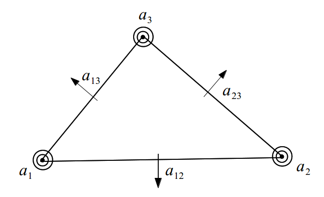
(a)

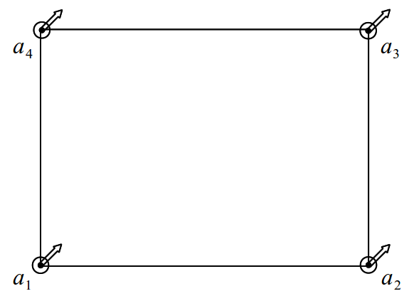
(b)

Figure 1. (A) Argyris element and (B) Bogner-Fox-Schmit element

Definition 3.1 (Argyris element [6, 9]).

The Argyris element is a triplet $(T,P_{5}(T),\Sigma_{T})$ where $T$ is a triangle, $P_{5}(T)$ denotes polynomials of degree $\leq 5$ in both the variables and the 21 degrees of freedom in $\Sigma_{T}$ are determined by the values of the unknown functions, its first order and second order derivatives at the three vertices and the normal derivatives at the midpoints of the three edges of $T$ (see Figure 1(A)).

Definition 3.2 (Bogner-Fox-Schmit element [9]).

Let $T\in\mathcal{T}_{h}$ be a rectangle with vertices $a_{i}=(x_{i},y_{i}),\>i=1,2,3,4$. The Bogner-Fox-Schmit element is a triplet $(T,Q_{3}(T),\Sigma_{T})$, where $Q_{3}(T)$ denotes polynomials of degree $\leq 3$ in both the variables and the degrees of freedom $\Sigma_{T}$ is defined by $\Sigma_{T}=\{p(a_{i}),\frac{\partial p}{\partial x}(a_{i}),\frac{\partial p}{\partial y}(a_{i}),\frac{\partial^{2}p}{\partial x\partial y}(a_{i}),\;1\leq i\leq 4\}$ (see Figure 1(B)).

The conforming $C^{1}$ finite element spaces associated with Argyris and Bogner-Fox-Schmit elements are contained in $C^{1}(\overline{\Omega})\cap H^{2}(\Omega)$. Define

$$V_{h} =\left\{v\in C^{1}(\overline{\Omega}):v|_{T}\in P_{T},\;\;\forall\,T\in\mathcal{T}_{h}\text{ with }v|_{\partial\Omega}=0,\frac{\partial v}{\partial\nu}\big{|}_{\partial\Omega}=0\right\}\subset H^{2}_{0}(\Omega),$$

where

$$P_{T} =\left\{\begin{array}[]{l l}P_{5}(T)&\text{for Argyris element},\\ Q_{3}(T)&\text{for Bogner-Fox-Schmit element}.\end{array}\right.$$

The discrete state and adjoint variables are sought in the finite dimensional space defined by ${\bf V}_{h}:={V_{h}}\times V_{h}$.

Lemma 3.1 (Interpolant [9]).

Let $\Pi_{h}:V\longrightarrow V_{h}$ be the Argyris or Bogner-Fox-Schmit nodal interpolation operator. Then for $\varphi\in H^{2+\gamma}(\Omega),$ with $\gamma\in(\frac{1}{2},1]$ denoting the index of elliptic regularity, it holds:

$$\|\varphi-\Pi_{h}\varphi\|_{m}\leq Ch^{\min\{k+1,\;2+\gamma\}-m}\|\varphi\|_{2+\gamma}\qquad\text{ for }m=0,1,2;$$ (3.1)

where $k=5$ (resp. 3) for the Argyris element (resp. Bogner-Fox-Schmit element).

3.2. Auxiliary problems for the state equations

Define an auxiliary continuous problem associated with the state equation as follows:

Seek $\Psi_{u}\in{\bf V}$ such that

$$A(\Psi_{u},\Phi)+B(\Psi_{u},\Psi_{u},\Phi)=(F+{\mathbf{C}}{\bf u},\Phi)\;\;\;\forall\,\Phi\in{\bf V},$$ (3.2)

where ${\bf u}=(u,0)$, $u\in L^{2}(\omega)$ is given.

A discrete conforming finite element approximation for this problem can be defined as:

Seek $\Psi_{u,h}\in{\bf V}_{h}$ such that

$$A(\Psi_{u,h},\Phi_{h})+B(\Psi_{u,h},\Psi_{u,h},\Phi_{h})=(F+{\mathbf{C}}{\bf u},\Phi_{h})\;\;\;\forall\,\Phi_{h}\in{\bf V}_{h}.$$ (3.3)

For a given $u\in L^{2}(\omega)$, (3.3) is not well-posed in general. The main results of this subsection are stated now.

Theorem 3.2.

Let $({\bar{\Psi}},{\bar{u}})\in{\bf V}\times L^{2}(\omega)$ be a nonsingular solution of (2.9). Then, there exist $\rho_{1},\rho_{2}>0$ and $h_{1}>0$ such that, for all $0<h<h_{1}$ and ${u}\in B_{\rho_{2}}({\bar{u}})$, (3.3) admits a unique solution in $B_{\rho_{1}}(\bar{\Psi})$.

Remark 3.3.

For $\rho>0$, ${u}\in B_{\rho}({\bar{u}})$ means that $\|u-{\bar{u}}\|_{L^{2}(\omega)}\leq\rho.$ Similarly, ${\Psi}\in B_{\rho}({\bar{\Psi}})\Longrightarrow\left|\!\left|\!\left|\Psi-{\bar{\Psi}}\right|\!\right|\!\right|_{2}\leq\rho.$

Theorem 3.4.

Let $({\bar{\Psi}},{\bar{u}})\in{\bf V}\times L^{2}(\omega)$ be a nonsingular solution of (2.9). Let $h_{1}$ and $\rho_{2}$ be defined as in Theorem 3.2. Then, for ${u}\in B_{\rho_{2}}({\bar{u}})$ and $0<h<h_{1}$, the solutions $\Psi_{u}$ and $\Psi_{u,h}$ of (3.2) and (3.3) satisfy the error estimates:

$$(a)\;\left|\!\left|\!\left|\Psi_{u}-\Psi_{u,h}\right|\!\right|\!\right|_{2}\leq Ch^{\gamma}\qquad(b)\;\;\left|\!\left|\!\left|\Psi_{u}-\Psi_{u,h}\right|\!\right|\!\right|_{1}\leq Ch^{2\gamma},$$ (3.4)

where $\gamma\in(1/2,1]$ denotes the index of elliptic regularity.

We proceed to establish several results which will be essential to prove Theorem 3.2. The proof of Theorem 3.4 follows from the error estimates for the approximation of von Kármán equations using conforming finite element methods; see [7, 21].

An auxiliary linear problem and discretization

For a given ${\bf g}=(g_{1},g_{2})\in{\bf V}^{\prime}$, let $T\in{\mathcal{L}}({\bf V}^{\prime},{\bf V})$ be defined by $T{\bf g}:=\boldsymbol{\xi}=(\xi_{1},\xi_{2})\in{\bf V}$ where $\boldsymbol{\xi}$ solves the system of biharmonic equations given by:

$$\Delta^{2}\xi_{1}=g_{1}\,\,\quad\mbox{ in }\Omega,$$ (3.5a)

$$\Delta^{2}\xi_{2}=g_{2}\quad\mbox{ in }\Omega,$$ (3.5b)

$$\xi_{1}=0,\,\frac{\partial\xi_{1}}{\partial\nu}=0\text{ and }\xi_{2}=0,\,\frac{\partial\xi_{2}}{\partial\nu}=0\text{ on }\partial\Omega.$$ (3.5c)

Equivalently, $\boldsymbol{\xi}\in{\bf V}$ solves $A(\boldsymbol{\xi},\Phi)=\big{\langle}{\bf g},\Phi\big{\rangle}_{{\bf V}^{\prime},{\bf V}}\quad\forall\Phi\in{\bf V}$.

Also, let $T_{h}\in{\mathcal{L}}({\bf V}^{\prime},{\bf V}_{h})$ be defined by $T_{h}{\bf g}:=\boldsymbol{\xi}_{h}$ if $\boldsymbol{\xi}_{h}\in{\bf V}_{h}$ solves the discrete problem

$$A(\boldsymbol{\xi}_{h},\Phi_{h})=\big{\langle}{\bf g},\Phi_{h}\big{\rangle}_{{\bf V}^{\prime},{\bf V}}\quad\forall\Phi_{h}\in{\bf V}_{h}.$$ (3.6)

Lemma 3.5.

(A bound for $T_{h}$) There exists a constant $C>0$, independent of $h$, such that

$$\|T_{h}\|_{{\mathcal{L}}({\bf V}^{\prime},{\bf V})}\leq C.$$

Proof.

The definition of $T_{h}{\bf g}$ along with coercivity property of the bilinear form $A(\cdot,\cdot)$ lead to the required result. ∎

Lemma 3.6.

[6](Error estimates) Let $\boldsymbol{\xi}$ and $\boldsymbol{\xi}_{h}$ solve (3.5) and (3.6) respectively. Then it holds:

$$\left|\!\left|\!\left|\boldsymbol{\xi}-\boldsymbol{\xi}_{h}\right|\!\right|\!\right|_{2}\leq Ch^{\gamma}\left|\!\left|\!\left|{\bf g}\right|\!\right|\!\right|_{-1}\quad\forall{\bf g}\in{{\bf H}}^{-1}(\Omega),$$ (3.7a)

$$\left|\!\left|\!\left|\boldsymbol{\xi}-\boldsymbol{\xi}_{h}\right|\!\right|\!\right|_{1}\leq Ch^{2\gamma}\left|\!\left|\!\left|{\bf g}\right|\!\right|\!\right|_{-1}\quad\forall{\bf g}\in{{\bf H}}^{-1}(\Omega),$$ (3.7b)

$\gamma\in(1/2,1]$ being the index of elliptic regularity. That is, $\left|\!\left|\!\left|(T-T_{h}){\bf g}\right|\!\right|\!\right|_{2}\leq Ch^{\gamma}\left|\!\left|\!\left|{\bf g}\right|\!\right|\!\right|_{-1}$ and $\left|\!\left|\!\left|(T-T_{h}){\bf g}\right|\!\right|\!\right|_{1}\leq Ch^{2\gamma}\left|\!\left|\!\left|{\bf g}\right|\!\right|\!\right|_{-1}$.

Remark 3.7.

When ${\bf g}=(g,0)$, we denote $T{\bf g}$ (resp. $T_{h}{\bf g}$) as $Tg$ (resp. $T_{h}g$), purely for notational convenience.

A nonlinear mapping and its properties

Define a nonlinear mapping ${\mathscr{N}}:{\bf V}\times L^{2}(\omega)\rightarrow{\bf V}$ by

$${\mathscr{N}}(\Psi,u):=\Psi+T[{\mathcal{B}}(\Psi)-(F+{\mathbf{C}}{\bf u})],\qquad{\bf u}=(u,0).$$

Now ${\mathscr{N}}(\Psi,u)=0$ if and only if $(\Psi,u)$ solves (2.9); that is, ${\mathcal{A}}\Psi+{\mathcal{B}}(\Psi)=F+{\mathbf{C}}{\bf u}\quad{\rm in}\;{\bf V}^{\prime}.$

Similarly, define a nonlinear mapping ${\mathscr{N}}_{h}:{\bf V}\times L^{2}(\omega)\rightarrow{\bf V}$ by

$${\mathscr{N}}_{h}(\Psi,u):=\Psi+T_{h}[{\mathcal{B}}(\Psi)-(F+{\mathbf{C}}{\bf u})],\qquad{\bf u}=(u,0).$$

Note that, ${\mathscr{N}}_{h}(\Psi,u)=0$ if and only if $\Psi\in{\bf V}_{h}$ and $\Psi=\Psi_{u,h}$ solves (3.3).

The derivative mapping $\partial_{\Psi}{\mathscr{N}}(\Psi,u)\;(\mbox{resp.}\;\partial_{\Psi}{\mathscr{N}}_{h}(\Psi,u))\in{\mathcal{L}}({\bf V})$ is defined by

$$\partial_{\Psi}{\mathscr{N}}(\Psi,u)(\Phi)=\Phi+T[{\mathcal{B}}^{\prime}(\Psi)\Phi]\quad\forall\Phi\in{\bf V}.$$

$$\big{(}\mbox{resp.}\;\partial_{\Psi}{\mathscr{N}}_{h}(\Psi,u)(\Phi)=\Phi+T_{h}[{\mathcal{B}}^{\prime}(\Psi)\Phi]\quad\forall\Phi\in{\bf V}.\big{)}$$

With definitions of nonsingular solution (see Definition 2.1), the linear mapping $T$ and the derivative mapping $\partial_{\Psi}{\mathscr{N}}(\Psi,u)$, we obtain the following result, the proof of which is skipped.

Lemma 3.8.

[8] If $({\bar{\Psi}},{\bar{u}})\in{\bf V}\times L^{2}(\omega)$ is a nonsingular solution of (2.1b), then $\partial_{\Psi}{\mathscr{N}}(\bar{\Psi},\bar{u})$ is an automorphism in ${\bf V}$. The converse also holds true.

We want to establish that if $({\bar{\Psi}},\bar{u})$ is a nonsingular solution, then the derivative mapping $\partial_{\Psi}{\mathscr{N}}_{h}(\cdot,\cdot)$ is an automorphism in ${\bf V}$, with respect to small perturbations of its arguments. That is, if $\left|\!\left|\!\left|{\Psi}-{\bar{\Psi}}\right|\!\right|\!\right|_{2}$ and $\|u-\bar{u}\|_{L^{2}(\omega)}$ are small enough, then $\partial_{\Psi}{\mathscr{N}}_{h}(\Psi,u)$ is an automorphism in ${\bf V}$. The next two lemmas will be useful in proving this result.

Lemma 3.9.

Let $\bar{\Psi}\in{\bf V}$ be a nonsingular solution of (2.9). Then, $\forall\epsilon>0$, $\exists h_{\epsilon}>0$ such that

$$\|T[B^{\prime}(\bar{\Psi})]-T_{h}[B^{\prime}(\Psi)]\|_{{\mathcal{L}}({\bf V})}<\epsilon\quad\forall\Psi\in B_{\rho_{\epsilon}}(\bar{\Psi}),$$ (3.8)

whenever $0<h<h_{\epsilon}$.

Proof.

For a fixed ${\bf z}\in{\bf V}$, let $T[B^{\prime}(\bar{\Psi}){\bf z}]=:{\boldsymbol{\theta}}(\bar{\Psi})\in{\bf V}$ and $T_{h}[B^{\prime}(\Psi){\bf z}]=:{\boldsymbol{\theta}}_{h}(\Psi)\in{\bf V}_{h}$. Then ${\boldsymbol{\theta}}(\bar{\Psi})$ and ${\boldsymbol{\theta}}_{h}(\Psi)$, respectively solve

$$A({\boldsymbol{\theta}}(\bar{\Psi}),\Phi) =\big{\langle}B^{\prime}(\bar{\Psi}){\bf z},\Phi\big{\rangle}_{{\bf V}^{\prime},{\bf V}}=B({\bar{\Psi}},{\bf z},\Phi)+B({\bf z},{\bar{\Psi}},\Phi)\quad\forall\Phi\in{\bf V},$$ (3.9)

$$A({\boldsymbol{\theta}}_{h}(\Psi),\Phi_{h}) =\big{\langle}B^{\prime}(\Psi){\bf z},\Phi_{h}\big{\rangle}_{{\bf V}^{\prime},{\bf V}}=B({\Psi},{\bf z},\Phi_{h})+B({\bf z},{\Psi},\Phi_{h})\quad\forall\Phi_{h}\in{\bf V}_{h}.$$ (3.10)

Let ${\boldsymbol{\theta}}_{h}({\bar{\Psi}})\in{\bf V}_{h}$ be the solution to the intermediate problem defined by

$$A({\boldsymbol{\theta}}_{h}(\bar{\Psi}),\Phi_{h})=\big{\langle}B^{\prime}(\bar{\Psi}){\bf z},\Phi_{h}\big{\rangle}_{{\bf V}^{\prime},{\bf V}}=B({\bar{\Psi}},{\bf z},\Phi_{h})+B({\bf z},{\bar{\Psi}},\Phi_{h})\quad\forall\Phi_{h}\in{\bf V}_{h}.$$ (3.11)

The triangle inequality yields

$$\left|\!\left|\!\left|{\boldsymbol{\theta}}(\bar{\Psi})-{\boldsymbol{\theta}}_{h}(\Psi)\right|\!\right|\!\right|_{2}\leq\left|\!\left|\!\left|{\boldsymbol{\theta}}(\bar{\Psi})-{\boldsymbol{\theta}}_{h}(\bar{\Psi})\right|\!\right|\!\right|_{2}+\left|\!\left|\!\left|{\boldsymbol{\theta}}_{h}(\bar{\Psi})-{\boldsymbol{\theta}}_{h}(\Psi)\right|\!\right|\!\right|_{2}.$$ (3.12)

To estimate the first term in the right hand side of (3.12), consider (3.9) and (3.11); use the facts that ${\bf V}_{h}\subset{\bf V}$, the error $({\boldsymbol{\theta}}(\bar{\Psi})-{\boldsymbol{\theta}}_{h}(\bar{\Psi}))$ is orthogonal to ${\bf V}_{h}$ in the energy norm, the coercivity of $A(\cdot,\cdot)$, the interpolation estimate given in Lemma 3.1 and the fact that ${\bar{\Psi}}\in{{\bf H}}^{2+\gamma}(\Omega)$ to obtain

$$\left|\!\left|\!\left|{\boldsymbol{\theta}}(\bar{\Psi})-{\boldsymbol{\theta}}_{h}(\bar{\Psi})\right|\!\right|\!\right|_{2}\leq Ch^{\gamma}\left|\!\left|\!\left|{\boldsymbol{\theta}}(\bar{\Psi})\right|\!\right|\!\right|_{2+\gamma}\leq Ch^{\gamma}\left|\!\left|\!\left|{\mathcal{B}}^{\prime}(\bar{\Psi}){\bf z}\right|\!\right|\!\right|_{-1}.$$ (3.13)

From definition of ${\mathcal{B}}^{\prime}(\bar{\Psi}){\bf z}$, (2.6) and the fact that $B(\cdot,\cdot,\cdot)$ is symmetric in first and second variables, it follows that

$$\left|\!\left|\!\left|{\mathcal{B}}^{\prime}(\bar{\Psi}){\bf z}\right|\!\right|\!\right|_{-1} =\sup\frac{\left|\big{\langle}{\mathcal{B}}^{\prime}(\bar{\Psi}){\bf z},\Phi\big{\rangle}\right|}{\left|\!\left|\!\left|\Phi\right|\!\right|\!\right|_{1}}$$

$$\leq\sup\frac{|B({\bar{\Psi}},{\bf z},\Phi)+B({\bf z},{\bar{\Psi}},\Phi)|}{\left|\!\left|\!\left|\Phi\right|\!\right|\!\right|_{1}}$$

$$\lesssim\left|\!\left|\!\left|\bar{\Psi}\right|\!\right|\!\right|_{2+\gamma}\left|\!\left|\!\left|{\bf z}\right|\!\right|\!\right|_{2}.$$ (3.14)

A substitution of (3.14) in (3.13) leads to

$$\left|\!\left|\!\left|{\boldsymbol{\theta}}(\bar{\Psi})-{\boldsymbol{\theta}}_{h}(\bar{\Psi})\right|\!\right|\!\right|_{2}\leq Ch^{\gamma}\left|\!\left|\!\left|\bar{\Psi}\right|\!\right|\!\right|_{2}\left|\!\left|\!\left|{\bf z}\right|\!\right|\!\right|_{2}.$$ (3.15)

To estimate the second term on the right hand side of (3.12), subtract (3.10) and (3.11), choose $\Phi_{h}={\boldsymbol{\theta}}_{h}(\bar{\Psi})-{\boldsymbol{\theta}}_{h}(\Psi)$, use (2.4) and (2.5) to obtain

$$\left|\!\left|\!\left|{\boldsymbol{\theta}}_{h}(\bar{\Psi})-{\boldsymbol{\theta}}_{h}(\Psi)\right|\!\right|\!\right|_{2}\leq C\left|\!\left|\!\left|\bar{\Psi}-{\Psi}\right|\!\right|\!\right|_{2}\left|\!\left|\!\left|{\bf z}\right|\!\right|\!\right|_{2}.$$ (3.16)

A use of (3.15) and (3.16) in (3.12) leads to the required result, when $h_{\epsilon}$ and $\rho_{\epsilon}$ are chosen sufficiently small. ∎

The next lemma is a standard result in Banach spaces and hence we refrain from providing a proof.

Lemma 3.10.

Let $X$ be a Banach space, $A\in{\mathcal{L}}(X)$ be invertible and $B\in{\mathcal{L}}(X)$. If $\|A-B\|_{{\mathcal{L}}(X)}<1/\|A^{-1}\|_{{\mathcal{L}}(X)}$, then $B$ is invertible. If $\|A-B\|_{{\mathcal{L}}(X)}<1/(2\|A^{-1}\|_{{\mathcal{L}}(X)})$ then $\|B^{-1}\|_{{\mathcal{L}}(X)}\leq 2\|A^{-1}\|_{{\mathcal{L}}(X)}$.

The following theorem is a consequence of Lemmas 3.9-3.10.

Theorem 3.11 (Invertibility of $\partial_{\Psi}{\mathscr{N}}_{h}(\Psi,u)$).

Let $({\bar{\Psi}},{\bar{u}})\in{\bf V}\times L^{2}(\omega)$ be a nonsingular solution of (2.1b). Then, there exist $h_{0}>0$ and $\rho_{0}>0$ such that, for all $0<h<h_{0}$ and all ${\Psi}\in B_{\rho_{0}}(\bar{\Psi})$, ${\mathscr{N}}_{h}(\Psi,u)$ is an automorphism in ${\bf V}$ and

$$\|{\partial_{\Psi}{\mathscr{N}}_{h}}({{\Psi}},{{u}})^{-1}\|_{{\mathcal{L}}({\bf V})}\leq 2\|{\partial_{\Psi}{\mathscr{N}}}({{\bar{\Psi}}},{{\bar{u}}})^{-1}\|_{{\mathcal{L}}({\bf V})}.$$

Proof.

Choose $h_{0}:=h_{\epsilon},\;\rho_{0}:=\rho_{\epsilon}$ and $\epsilon=\frac{1}{2\|{\partial_{\Psi}{\mathscr{N}}}({{\bar{\Psi}}},{{\bar{u}}})^{-1}\|_{{\mathcal{L}}({\bf V})}}$ in Lemma 3.9.

For every $0<h<h_{0}$ and for all $\Psi\in B_{\rho_{0}}({\bar{\Psi}})$, the definitions of the derivatives of $\partial_{\Psi}{\mathscr{N}}$, $\partial_{\Psi}{\mathscr{N}}_{h}$ and (3.8) yield

$$\|{\partial_{\Psi}{\mathscr{N}}}({{\bar{\Psi}}},{{\bar{u}}})-{\partial_{\Psi}{\mathscr{N}_{h}}}({{\Psi}},{{u}})\|_{{\mathcal{L}}({\bf V})} =\|T[B^{\prime}(\bar{\Psi})]-T_{h}[B^{\prime}(\Psi)]\|_{{\mathcal{L}}({\bf V})}<\epsilon.$$

Now, an application of Lemma 3.10 yields the required result. ∎

We now proceed to provide a proof Theorem 3.2, which is the main result of this subsection.

Proof of Theorem 3.2:

Let $({\bar{\Psi}},{\bar{u}})\in{\bf V}\times L^{2}(\omega)$ be a nonsingular solution of (2.9).

We need to establish that there exist $\rho_{1},\rho_{2}>0$ and $h_{1}>0$ such that, for all $0<h<h_{1}$ and ${u}\in B_{\rho_{2}}({\bar{u}})$, ${\mathscr{N}}_{h}(\Psi,u)=0$ admits a unique solution in $B_{\rho_{1}}(\bar{\Psi})$.

Let $\rho_{0}$ and $h_{0}$ be the positive constants as defined in Theorem 3.11. For $\rho\leq\rho_{0}$, $h\leq h_{0}$ and $u\in B_{\rho_{2}}({\bar{u}})$, define a mapping ${\mathscr{G}}(\cdot,u):B_{\rho}({\bar{\Psi}})\rightarrow{\bf V}$ by

$${\mathscr{G}}(\Psi,u)=\Psi-[\partial_{\Psi}{\mathscr{N}}_{h}({\bar{\Psi}},{\bar{u}})]^{-1}{\mathscr{N}}_{h}(\Psi,u).$$

Any fixed point of ${\mathscr{G}}(\cdot,u)$ is a solution of the discrete nonlinear problem ${\mathscr{N}}_{h}(\Psi,u)=0$. In the next two steps, we establish that (i) ${\mathscr{G}}(\cdot,u)$ maps $B_{\rho}({\bar{\Psi}})$ into itself; and (ii) ${\mathscr{G}}(\cdot,u)$ is a strict contraction, if $\rho$ is small enough.

Step 1: The definition of ${\mathscr{G}}(\cdot,u)$, an addition of the zero term ${\mathscr{N}}({\bar{\Psi}},{\bar{u}})$, an addition and subtraction of an intermediate term and the Taylor’s Theorem yield

$$\left|\!\left|\!\left|{\mathscr{G}}(\Psi,u)-{\bar{\Psi}}\right|\!\right|\!\right|_{2} =\left|\!\left|\!\left|(\Psi-{\bar{\Psi}})-[\partial_{\Psi}{\mathscr{N}}_{h}({\bar{\Psi}},{\bar{u}})]^{-1}{\mathscr{N}}_{h}(\Psi,u)\right|\!\right|\!\right|_{2}$$

$$\leq\left|\!\left|\!\left|[\partial_{\Psi}{\mathscr{N}}_{h}({\bar{\Psi}},{\bar{u}})]^{-1}\left\{[\partial_{\Psi}{\mathscr{N}}_{h}({\bar{\Psi}},{\bar{u}})](\Psi-{\bar{\Psi}})-[{\mathscr{N}}_{h}(\Psi,u)-{\mathscr{N}}_{h}({\bar{\Psi}},u)]\right\}\right|\!\right|\!\right|_{2}$$

$$\qquad+\left|\!\left|\!\left|[\partial_{\Psi}{\mathscr{N}}_{h}({\bar{\Psi}},{\bar{u}})]^{-1}[{\mathscr{N}}(\bar{\Psi},\bar{u})-{\mathscr{N}}_{h}(\bar{\Psi},u)]\right|\!\right|\!\right|_{2}.$$ (3.17)

A use of Theorem 3.11, Taylor formula for the second expression in the first term of the right hand side of (3.17) along with the fact that the expression for the derivative $\partial_{\Psi}$ is independent of $u$ yields for $\Psi_{t}=\bar{\Psi}+t(\Psi-\bar{\Psi}),\;0<t<1$,

$$\left|\!\left|\!\left|{\mathscr{G}}(\Psi,u)-{\bar{\Psi}}\right|\!\right|\!\right|_{2} \leq C\left|\!\left|\!\left|\partial_{\Psi}{\mathscr{N}}_{h}({\bar{\Psi}},{\bar{u}})](\Psi-{\bar{\Psi}})-\int_{0}^{1}\partial_{\Psi}{\mathscr{N}}_{h}({\Psi_{t}},u)(\Psi-{\bar{\Psi}})\right|\!\right|\!\right|_{2}$$

$$\quad+C\left|\!\left|\!\left|[{\mathscr{N}}(\bar{\Psi},\bar{u})-{\mathscr{N}}_{h}(\bar{\Psi},u)]\right|\!\right|\!\right|_{2}.$$

With definitions of ${\mathscr{N}}(\cdot,\cdot)$ and ${\mathscr{N}}_{h}(\cdot,\cdot)$, and the triangle inequality in the above expression, we obtain

$$\left|\!\left|\!\left|{\mathscr{G}}(\Psi,u)-{\bar{\Psi}}\right|\!\right|\!\right|_{2}\leq C\int_{0}^{1}\left|\!\left|\!\left|\partial_{\Psi}{\mathscr{N}}_{h}({\bar{\Psi}},{\bar{u}})]-\partial_{\Psi}{\mathscr{N}}_{h}({\Psi_{t}},u)\right|\!\right|\!\right|_{2}\>dt\times\left|\!\left|\!\left|\Psi-{\bar{\Psi}}\right|\!\right|\!\right|_{2}$$

$$+\;C\left|\!\left|\!\left|(T-T_{h})({\mathcal{B}}(\bar{\Psi})-f)\right|\!\right|\!\right|_{2}+C\left|\!\left|\!\left|(T-T_{h})({\mathcal{C}}{\bar{u}})\right|\!\right|\!\right|_{2}$$

$$+\;C\left|\!\left|\!\left|T_{h}({\mathcal{C}}{\bar{u}}-{\mathcal{C}}u)\right|\!\right|\!\right|_{2}=:T_{1}+T_{2}+T_{3}+T_{4}.$$ (3.18)

We now estimate the terms $T_{1}$ to $T_{4}$. With the definition of $\partial_{\Psi}{\mathscr{N}}_{h}(\cdot,\cdot)$, Lemma 3.5, the definition of ${\mathcal{B}}^{\prime}(\cdot)$ and (2.5), it yields

$$\|\partial_{\Psi}{\mathscr{N}}_{h}({\bar{\Psi}},{\bar{u}})-\partial_{\Psi}{\mathscr{N}}_{h}({\bar{\Psi}+t(\Psi-\bar{\Psi})},u)\|_{\mathcal{L}(V)}\> =\|T_{h}({\mathcal{B}}^{\prime}({\bar{\Psi}}+t(\Psi-\bar{\Psi})))-T_{h}({\mathcal{B}}^{\prime}(\bar{\Psi}))\|_{\mathcal{L}(V)}$$

$$\leq C\left|\!\left|\!\left|\Psi-\bar{\Psi}\right|\!\right|\!\right|_{2}.$$ (3.19)

A use of the fact that $\bar{\Psi}\in{{\bf H}}^{2+\gamma}(\Omega)$, ${\mathcal{B}}(\bar{\Psi})\in{{\bf H}}^{-1}(\Omega)$ and $f\in H^{-1}(\Omega)$ along with (3.7) lead to an estimate for $T_{2}$ as

$$\left|\!\left|\!\left|(T-T_{h})({\mathcal{B}}(\bar{\Psi})-f)\right|\!\right|\!\right|_{2}\leq Ch^{\gamma}(\left|\!\left|\!\left|\bar{\Psi}\right|\!\right|\!\right|_{2}^{2}+\|f\|_{H^{-1}(\Omega)})),$$ (3.20)

where $\gamma\in(1/2,1]$ is the elliptic regularity index. Since $\bar{u}\in L^{2}(\omega)$, $T_{3}$ can also be estimated using (3.7) as

$$\left|\!\left|\!\left|(T-T_{h})({\mathcal{C}}{\bar{u}})\right|\!\right|\!\right|_{2}\leq Ch^{\gamma}\|\bar{u}\|_{L^{2}(\omega)}.$$ (3.21)

The boundedness of $T_{h}$ from Lemma 3.5 leads to

$$\left|\!\left|\!\left|T_{h}({\mathcal{C}}{\bar{u}}-{\mathcal{C}}u)\right|\!\right|\!\right|_{2}\leq C\left|\!\left|\!\left|{\mathcal{C}}{\bar{u}}-{\mathcal{C}}u\right|\!\right|\!\right|\leq C\|\bar{u}-u\|_{L^{2}(\omega)}.$$ (3.22)

The substitutions of (3.19)-(3.22) in (3.2) yield

$$\left|\!\left|\!\left|{\mathscr{G}}(\Psi,u)-{\bar{\Psi}}\right|\!\right|\!\right|_{2}\leq\hat{C}(h^{\gamma}+\rho^{2}).$$

Choose $\hat{\rho}_{1}\leq\min\left\{\rho_{0},\frac{1}{2\hat{C}}\right\},\;\hat{\rho}_{2}={\hat{\rho}}_{1}^{2},$ and $\hat{h}_{1}=\min\left\{{h_{0}^{1/\gamma},\left(\frac{\hat{\rho}_{1}}{2\hat{C}}\right)^{1/\gamma}}\right\}$. For all $0<h<{\hat{h}}_{1}$ and all $u\in B_{\hat{\rho}_{2}}(\bar{u})$, ${\mathscr{G}}(\Psi,u)$ is a mapping from $B_{{\hat{\rho}}_{1}}(\bar{\Psi})$ into itself.

Step 2: Let $\Psi_{1},\Psi_{2}\in B_{{\hat{\rho}}_{1}}(\bar{\Psi}),\;$ $0<h<{\hat{h}}_{1}$ and $u\in B_{\hat{\rho}_{2}}(\bar{u})$. The definition of the mapping ${\mathscr{G}}(\cdot,u)$ and standard calculations lead to

$$\left|\!\left|\!\left|{\mathscr{G}}(\Psi_{1},u)-{\mathscr{G}}(\Psi_{2},u)\right|\!\right|\!\right|_{2}=\left|\!\left|\!\left|\Psi_{1}-\Psi_{2}-[\partial_{\Psi}{\mathscr{N}}_{h}({\bar{\Psi}},{\bar{u}})]^{-1}\left\{{\mathscr{N}}_{h}(\Psi_{1},u)-{\mathscr{N}}_{h}(\Psi_{2},u)\right\}\right|\!\right|\!\right|_{2}$$

$$=\left|\!\left|\!\left|[\partial_{\Psi}{\mathscr{N}}_{h}({\bar{\Psi}},{\bar{u}})]^{-1}\left\{\partial_{\Psi}{\mathscr{N}}_{h}({\bar{\Psi}},{\bar{u}})(\Psi_{1}-\Psi_{2})-\int_{0}^{1}\partial_{\Psi}{\mathscr{N}}_{h}(\Psi_{2}+t(\Psi_{1}-\Psi_{2}),u)(\Psi_{1}-\Psi_{2})\>dt\right\}\right|\!\right|\!\right|_{2}.$$ (3.23)

Now a use of Theorem 3.11 and a repetition of arguments used in (3.19) lead to the result that, there exists a positive constant ${\tilde{C}}$ independent of ${\hat{\rho}}_{1}$ and $h$ such that

$$\left|\!\left|\!\left|{\mathscr{G}}(\Psi_{1},u)-{\mathscr{G}}(\Psi_{2},u)\right|\!\right|\!\right|_{2}\leq{\tilde{C}}{\hat{\rho}}_{1}^{2}.$$ (3.24)

A choice of $\rho_{1}=\min\left\{\rho_{0},\frac{1}{2\hat{C}},\frac{1}{\sqrt{2\tilde{C}}}\right\}$, $\rho_{2}=\rho_{1}^{2}$, and $h_{1}=\min\left\{{h_{0}^{1/\gamma},\left(\frac{\rho_{1}}{2\hat{C}}\right)^{1/\gamma}}\right\}$ leads to the result that for all $0<h<h_{1}$ and $u\in B_{\rho_{2}}(\bar{u})$, ${\mathscr{G}}(\cdot,u)$ is a strict contraction in $B_{\rho_{1}}({\bar{\Psi}})$.

This concludes the proof of Theorem 3.2. $\Box$

We have established that, for $0<h<h_{1}$, $u\in B_{\rho_{2}}({\bar{u}})$, ${\mathscr{N}}_{h}(\Psi_{h},u)=0$ admits a unique solution $\Psi_{u,h}\in B_{\rho_{1}}({\bar{\Psi}})\cap{\bf V}_{h}$. Also, $\partial_{\Psi}{\mathscr{N}}_{h}(\Psi_{u,h},u)$ is an automorphism in ${\bf V}$. Hence, the mapping $G_{h}:B_{\rho_{2}}({\bar{u}})\rightarrow B_{\rho_{1}}({\bar{\Psi}})\cap{\bf V}_{h}$ defined by $G_{h}(u)=\Psi_{u,h}$ satisfies ${\mathscr{N}}_{h}(G_{h}(u),u)=0$. The implicit theorem yields that $G_{h}$ is of class $C^{\infty}$ in the interior of the ball.

This fact, along with Theorem 3.4 yields the following lemma.

Lemma 3.12.

For $u,\>{\hat{u}}\in B_{\rho_{2}}({\bar{u}}),\>0<h<h_{1}$, the solutions $\Psi_{u}$ and $\Psi_{{\hat{u}},h}$ to (3.2) and (3.3), with controls chosen as $u$ and ${\hat{u}}$ respectively, satisfy

$$\left|\!\left|\!\left|\Psi_{u}-\Psi_{{\hat{u}},h}\right|\!\right|\!\right|_{2}\leq C(h^{\gamma}+\|u-{\hat{u}}\|_{L^{2}(\omega)}),\;$$

$\gamma\in(1/2,1]$ being the elliptic regularity index.

Proof.

The triangle inequality yields

$$\left|\!\left|\!\left|\Psi_{u}-\Psi_{{\hat{u}},h}\right|\!\right|\!\right|_{2}\leq\left|\!\left|\!\left|\Psi_{u}-\Psi_{u,h}\right|\!\right|\!\right|_{2}+\left|\!\left|\!\left|\Psi_{u,h}-\Psi_{{\hat{u}},h}\right|\!\right|\!\right|_{2}.$$ (3.25)

Theorem 3.4 yields the estimate for the first term on the right hand side of (3.25) as

$$\left|\!\left|\!\left|\Psi_{u}-\Psi_{u,h}\right|\!\right|\!\right|_{2}\leq Ch^{\gamma}.$$

From the expression ${\mathscr{N}}_{h}(G_{h}(u),u)=0$ and the definition of ${\mathscr{N}}_{h}$, we obtain

$$G^{\prime}_{h}(u)(v)=-[\partial_{\Psi}{\mathscr{N}}_{h}(\Psi_{u,h},u)]^{-1}T_{h}({\mathcal{C}}v),$$

where $u$ belongs to the interior of $B_{\rho_{2}}({\bf u})$.

Hence Lemma 3.5 and Theorem 3.11 yield

$$\left|\!\left|\!\left|\Psi_{u,h}-\Psi_{{\hat{u}},h}\right|\!\right|\!\right|_{2} =\left|\!\left|\!\left|G_{h}(u)-G_{h}({\hat{u}})\right|\!\right|\!\right|_{2}$$

$$=\left|\!\left|\!\left|\int_{0}^{1}[\partial_{\Psi}{\mathscr{N}}_{h}(\Psi_{h}({u_{t}}),u_{t})]^{-1}T_{h}({\mathcal{C}}(u-{\hat{u}}))\right|\!\right|\!\right|_{2}$$

$$\leq C\|u-{\hat{u}}\|_{L^{2}(\omega)},$$ (3.26)

with $u_{t}={\hat{u}}+t(u-\hat{u})$. A substitution of the estimate in (3.25) yields the required result.

∎

3.3. Auxiliary discrete problem for the adjoint equations

Define an auxiliary continuous problem associated with the adjoint equations as follows:

Seek $\Theta_{u}\in{\bf V}$ such that

$$A(\Phi,\Theta_{u})+B(\Psi_{u},\Phi,\Theta_{u})+B(\Phi,\Psi_{u},\Theta_{u})=(\Psi_{u}-\Psi_{d},\Phi)\;\;\;\forall\,\Phi\in{\bf V},$$ (3.27)

where $\Psi_{u}\in{\bf V}$ is the solution of (3.2) and $\Psi_{d}$ is given. A conforming finite element discretization for (3.27) is defined as:

Seek $\Theta_{u,h}\in{\bf V}_{h}$ such that

$$A(\Phi_{h},\Theta_{u,h})+B(\Psi_{u,h},\Phi_{h},\Theta_{u,h})+B(\Phi_{h},\Psi_{u,h},\Theta_{u,h})=(\Psi_{u,h}-\Psi_{d},\Phi_{h})\;\;\;\forall\,\Phi_{h}\in{\bf V}_{h}.$$ (3.28)

The main results of this subsection will be on the existence of solution of the discrete adjoint problem in (3.28) and its error estimates. They are stated now.

Theorem 3.13.

Let $({\bar{\Psi}},{\bar{u}})\in{\bf V}\times L^{2}(\omega)$ be a nonsingular solution of (2.9). Then, there exist $0<\rho_{3}\leq\rho_{2}$ and $h_{3}>0$ such that, for all $0<h\leq h_{3}$ and ${u}\in B_{\rho_{3}}({\bar{u}})$, (3.28) admits a unique solution.

Theorem 3.14.

Let $({\bar{\Psi}},{\bar{u}})\in{\bf V}\times L^{2}(\omega)$ be a nonsingular solution of (2.9). Then, for ${u}\in B_{\rho_{3}}({\bar{u}})$ and $0<h<h_{3}$, the solutions $\Theta_{u}$ and $\Theta_{u,h}$ of (3.27) and (3.28) satisfy the error estimates:

$$(a)\;\left|\!\left|\!\left|\Theta_{u}-\Theta_{u,h}\right|\!\right|\!\right|_{2}\leq Ch^{\gamma}\qquad(b)\;\;\left|\!\left|\!\left|\Theta_{u}-\Theta_{u,h}\right|\!\right|\!\right|_{1}\leq Ch^{2\gamma},$$ (3.29)

where $\gamma\in(1/2,1]$ denotes the index of elliptic regularity.

A linear mapping and its properties:

As in the case of the derivative mapping defined in the previous subsection for state equations, define the linear mapping ${\mathscr{F}}_{\Psi}(\mbox{resp. }{\mathscr{F}}_{\Psi,h})\in{\mathcal{L}}({\bf V})$ by

$${\mathscr{F}}_{\Psi}(\Phi)=\Phi+T[{\mathcal{B}}^{\prime}(\Psi)^{*}\Phi]\quad\forall\Phi\in{\bf V},$$

$$\left({\rm resp.}\;{\mathscr{F}}_{\Psi,h}(\Phi)=\Phi+T_{h}[{\mathcal{B}}^{\prime}(\Psi)^{*}\Phi]\quad\forall\Phi\in{\bf V}\right)$$

where ${\mathcal{B}}^{\prime}(\Psi)^{*}$ is the adjoint operator corresponding to ${\mathcal{B}}^{\prime}(\Psi)$ (see (2.11)).

The next lemma is easy to establish and hence the proof is skipped.

Lemma 3.15.

The mapping ${\mathscr{F}}_{\Psi}$ is an automorphism in ${\bf V}$ if and only if $\Psi\in{\bf V}$ is a nonsingular solution of (2.1b).

Proof of Theorem 3.13:

Proceeding as in the proof of Theorem 3.11, we can assume that $h_{0}$ is chosen so that, for all $0<h<h_{0}$ and all ${\Psi}\in B_{\rho_{0}}({\bar{\Psi}})$, ${\mathscr{F}}_{\Psi,h}$ is an automorphism in ${\bf V}$. In particular, by using Lemma 3.12, there exist $0<h_{3}\leq h_{2}$ and $0<\rho_{3}\leq\rho_{2}$ such that, for all $0<h\leq h_{3}$ and all $u\in B_{\rho_{3}}({\bar{u}})$, ${\mathscr{F}}_{\Psi_{u,h},h}$ is an automorphism in ${\bf V}$ and

$$\|{\mathscr{F}}_{\Psi_{u,h},h}^{-1}\|_{\mathcal{L}({\bf V})}\leq 2\|{\mathscr{F}}_{\bar{\Psi}}^{-1}\|_{\mathcal{L}({\bf V})}.$$

We can also assume that ${\mathscr{F}}_{\Psi_{u}}$ is an automorphism in ${\bf V}$ for all $u\in B_{\rho_{3}}({\bar{u}})$.

Now we establish that $\Theta_{u,h}\in{\bf V}_{h}$ is a solution of (3.28) if and only if ${\mathscr{F}}_{\Psi_{u,h},h}(\Theta_{u,h})={\boldsymbol{\eta}}_{h}$, where ${\boldsymbol{\eta}}_{h}\in{\bf V}_{h}$ satisfies $T_{h}(\Psi_{u}-\Psi_{d})={\boldsymbol{\eta}}_{h}$.

With definitions of ${\mathscr{F}}_{\Psi_{u,h},h}$ and the operator $T_{h}$, it yields

$${\mathscr{F}}_{\Psi_{u,h},h}(\Theta_{u,h}) ={\boldsymbol{\eta}}_{h}\Longleftrightarrow\Theta_{u,h}+T_{h}[{\mathcal{B}}^{\prime}(\Psi_{u,h})^{*}\Theta_{u,h}]={\boldsymbol{\eta}}_{h}$$

$$\Longleftrightarrow A(\Theta_{u,h},\Phi_{h})+\big{\langle}{\mathcal{B}}^{\prime}(\Psi_{u,h})^{*}\Theta_{u,h},\Phi_{h}\big{\rangle}_{{\bf V}^{\prime},{\bf V}}=(\Psi_{u,h}-\Psi_{d},\Phi_{h})\;\forall\Phi_{h}\in{\bf V}_{h}.$$

That is, $\Theta_{u,h}\in{\bf V}_{h}$ solves (3.28). $\Box$

Proof of Theorem 3.14:

The problem under consideration being linear, it is straight forward to obtain the required estimates. We will sketch the steps of the proof.

The space ${\bf V}_{h}$ is a subspace of ${\bf V}$ and hence (3.27) holds true for test functions in ${\bf V}_{h}$.

The definition of ${\mathscr{F}}_{\Psi_{u,h},h}$, and of the continuous and discrete adjoint problems lead to

$${\mathscr{F}}_{\Psi_{u,h},h}(\Theta_{u}-\Theta_{u,h})={\mathscr{F}}_{\Psi_{u,h},h}(\Theta_{u})-{\mathscr{F}}_{\Psi_{u,h},h}(\Theta_{u,h})$$

$$=\Theta_{u}+T_{h}[B^{\prime}(\Psi_{u,h})^{*}\Theta_{u}]-T_{h}(\Psi_{u,h}-\Psi_{d})$$

$$=T(\Psi_{u}-\Psi_{d})-T[B^{\prime}(\Psi_{u})^{*}\Theta_{u}]+T_{h}[B^{\prime}(\Psi_{u,h})^{*}\Theta_{u}]-T_{h}(\Psi_{u,h}-\Psi_{d})$$

$$=T(\Psi_{u}-\Psi_{u,h})+(T-T_{h})(\Psi_{u,h}-\Psi_{d}-B^{\prime}(\Psi_{u,h})^{*}\Theta_{u})+T[B^{\prime}(\Psi_{u,h})^{*}\Theta_{u}-B^{\prime}(\Psi_{u})^{*}\Theta_{u}].$$

Since $F_{\Psi_{u,h},h}$ is an automorphism in ${\bf V}_{h}$, the boundedness of $T$ leads to

$$\left|\!\left|\!\left|\Theta_{u}-\Theta_{u,h}\right|\!\right|\!\right|_{2} \lesssim\left|\!\left|\!\left|\Psi_{u}-\Psi_{u,h}\right|\!\right|\!\right|_{2}+\|T-T_{h}\|\left|\!\left|\!\left|\Psi_{u,h}-\Psi_{d}-B^{\prime}(\Psi_{u,h})^{*}\Theta\right|\!\right|\!\right|_{2}$$

$$\quad+\|B^{\prime}(\Psi_{u,h}-\Psi_{u})^{*}\Theta_{u}\|_{{\bf V}^{\prime}}.$$

A use of Theorem 3.4(a) and Lemma 3.6 leads to the first estimate in (3.29).

To establish the second estimate in (3.29), define an auxiliary problem and its discretization.

For all ${\bf g}\in{{\bf H}}^{-1}(\Omega)$, let ${\boldsymbol{\chi}}_{\bf g}\in{\bf V}$ and ${\boldsymbol{\chi}}_{{\bf g},h}\in{\bf V}_{h}$ be the solutions to the equations

$$A({\boldsymbol{\chi}}_{\bf g},\Phi)+B(\Psi_{u},{\boldsymbol{\chi}}_{\bf g},\Phi)+B({\boldsymbol{\chi}}_{\bf g},\Psi_{u},\Phi)=\langle{\bf g},\Phi\rangle\quad\forall\Phi\in{\bf V}.$$ (3.30)

$$A({\boldsymbol{\chi}}_{{\bf g},h},\Phi_{h})+B(\Psi_{u},{\boldsymbol{\chi}}_{{\bf g},h},\Phi_{h})+B({\boldsymbol{\chi}}_{{\bf g},h},\Psi_{u},\Phi_{h})=\langle{\bf g},\Phi_{h}\rangle\quad\forall\Phi_{h}\in{\bf V}_{h}.$$ (3.31)

The well-posedness of (3.30) implies that $\left|\!\left|\!\left|{\boldsymbol{\chi}}_{\bf g}\right|\!\right|\!\right|_{2}\lesssim\left|\!\left|\!\left|{\bf g}\right|\!\right|\!\right|_{-1}$ and $\left|\!\left|\!\left|{\boldsymbol{\chi}}_{\bf g}\right|\!\right|\!\right|_{2+\gamma}\lesssim\left|\!\left|\!\left|{\bf g}\right|\!\right|\!\right|_{-1}$. By proceeding as as in the proof of (a), we can establish that

$$\left|\!\left|\!\left|{\boldsymbol{\chi}}_{\bf g}-{\boldsymbol{\chi}}_{{\bf g},h}\right|\!\right|\!\right|_{2}\leq Ch^{\gamma}\left|\!\left|\!\left|{\bf g}\right|\!\right|\!\right|_{-1},$$ (3.32)

where the constant $C$ depends on $\left|\!\left|\!\left|\Psi\right|\!\right|\!\right|_{2}$, and $\gamma\in(1/2,1]$ is the index of elliptic regularity.

From (3.27) and (3.28), it follows that

$$\begin{array}[]{l}\displaystyle A(\Phi_{h},\Theta_{u}-\Theta_{u,h})+B(\Psi_{u},\Phi_{h},\Theta_{u})+B(\Phi_{h},\Psi_{u},\Theta_{u})\vspace{2.mm}\\ -B(\Psi_{u,h},\Phi_{h},\Theta_{u,h})-B(\Phi_{h},\Psi_{u,h},\Theta_{u,h})=(\Psi_{u}-\Psi_{u,h},\Phi_{h})\quad\mbox{for all}\ \Phi_{h}\in{\bf V}_{h}.\end{array}$$ (3.33)

Choose $\Phi=\Theta_{u}-\Theta_{u,h}$ in (3.30) and adjustment of terms yield

$$({\bf g},\Theta_{u}-\Theta_{u,h}) =A({\boldsymbol{\chi}}_{\bf g}-{\boldsymbol{\chi}}_{{\bf g},h},\Theta_{u}-\Theta_{u,h})+B(\Psi_{u},{\boldsymbol{\chi}}_{\bf g}-{\boldsymbol{\chi}}_{{\bf g},h},\Theta_{u}-\Theta_{u,h})$$

$$\;\;+B({\boldsymbol{\chi}}_{\bf g}-{\boldsymbol{\chi}}_{{\bf g},h},\Psi_{u},\Theta_{u}-\Theta_{u,h})+B(\Psi_{u},{\boldsymbol{\chi}}_{{\bf g},h},\Theta_{u}-\Theta_{u,h})$$

$$\;\;+B({\boldsymbol{\chi}}_{{\bf g},h},\Psi_{u},\Theta_{u}-\Theta_{u,h})+A({\boldsymbol{\chi}}_{{\bf g},h},\Theta_{u}-\Theta_{u,h}).$$ (3.34)

Choose $\Phi_{h}={\boldsymbol{\chi}}_{{\bf g},h}$ in (3.33) and combine with (3.34) to obtain

$$({\bf g},\Theta_{u}-\Theta_{u,h}) =A({\boldsymbol{\chi}}_{\bf g}-{\boldsymbol{\chi}}_{{\bf g},h},\Theta_{u}-\Theta_{u,h})+B(\Psi_{u},{\boldsymbol{\chi}}_{\bf g}-{\boldsymbol{\chi}}_{{\bf g},h},\Theta_{u}-\Theta_{u,h})$$

$$\quad+B({\boldsymbol{\chi}}_{\bf g}-{\boldsymbol{\chi}}_{{\bf g},h},\Psi_{u},\Theta_{u}-\Theta_{u,h})+B(\Psi_{u,h}-\Psi_{u},{\boldsymbol{\chi}}_{{\bf g},h},\Theta_{u,h})$$

$$\quad+B({\boldsymbol{\chi}}_{{\bf g},h},\Psi_{u,h}-\Psi_{u},\Theta_{u,h})+(\Psi_{u}-\Psi_{u,h},{\boldsymbol{\chi}}_{{\bf g},h})$$

$$=A({\boldsymbol{\chi}}_{\bf g}-{\boldsymbol{\chi}}_{{\bf g},h},\Theta_{u}-\Theta_{u,h})+B(\Psi_{u},{\boldsymbol{\chi}}_{\bf g}-{\boldsymbol{\chi}}_{{\bf g},h},\Theta_{u}-\Theta_{u,h})$$

$$\quad+B({\boldsymbol{\chi}}_{\bf g}-{\boldsymbol{\chi}}_{{\bf g},h},\Psi_{u},\Theta_{u}-\Theta_{u,h})+B(\Psi_{u,h}-\Psi_{u},{\boldsymbol{\chi}}_{{\bf g},h}-{\boldsymbol{\chi}}_{\bf g},\Theta_{u,h})$$

$$\quad+B(\Psi_{u,h}-\Psi_{u},{\boldsymbol{\chi}}_{\bf g},\Theta_{u,h})+B({\boldsymbol{\chi}}_{{\bf g},h}-{\boldsymbol{\chi}}_{\bf g},\Psi_{u,h}-\Psi_{u},\Theta_{u,h})$$

$$\quad+B({\boldsymbol{\chi}}_{\bf g},\Psi_{u,h}-\Psi_{u},\Theta_{u,h})+(\Psi_{u}-\Psi_{u,h},{\boldsymbol{\chi}}_{{\bf g},h}).$$ (3.35)

A choice of ${\bf g}=-\Delta(\Theta_{u}-\Theta_{u,h})$ in the above equation (3.35) and then integration by parts, and a use of boundedness properties (2.4), (2.5) and (2.6) lead to

$$\left|\!\left|\!\left|\Theta_{u}-\Theta_{u,h}\right|\!\right|\!\right|_{1}^{2} \lesssim\left|\!\left|\!\left|{\boldsymbol{\chi}}_{\bf g}-{\boldsymbol{\chi}}_{{\bf g},h}\right|\!\right|\!\right|_{2}\left|\!\left|\!\left|\Theta_{u}-\Theta_{u,h}\right|\!\right|\!\right|_{2}+\left|\!\left|\!\left|\Psi_{u,h}-\Psi_{u}\right|\!\right|\!\right|_{1}\left|\!\left|\!\left|{\boldsymbol{\chi}}_{\bf g}\right|\!\right|\!\right|_{2+\gamma}+\left|\!\left|\!\left|\Psi_{u,h}-\Psi_{u}\right|\!\right|\!\right|\left|\!\left|\!\left|{\boldsymbol{\chi}}_{{\bf g},h}\right|\!\right|\!\right|$$

$$\lesssim\left|\!\left|\!\left|{\boldsymbol{\chi}}_{\bf g}-{\boldsymbol{\chi}}_{{\bf g},h}\right|\!\right|\!\right|_{2}\left|\!\left|\!\left|\Theta_{u}-\Theta_{u,h}\right|\!\right|\!\right|_{2}+\left|\!\left|\!\left|\Psi_{u,h}-\Psi_{u}\right|\!\right|\!\right|_{1}\left|\!\left|\!\left|{\boldsymbol{\chi}}_{\bf g}\right|\!\right|\!\right|_{2+\gamma}$$

$$\quad+\left|\!\left|\!\left|\Psi_{u,h}-\Psi_{u}\right|\!\right|\!\right|\left|\!\left|\!\left|{\boldsymbol{\chi}}_{\bf g}-{\boldsymbol{\chi}}_{{\bf g},h}\right|\!\right|\!\right|+\left|\!\left|\!\left|\Psi_{u,h}-\Psi_{u}\right|\!\right|\!\right|\left|\!\left|\!\left|{\boldsymbol{\chi}}_{\bf g}\right|\!\right|\!\right|.$$ (3.36)

Note that $\left|\!\left|\!\left|{\bf g}\right|\!\right|\!\right|_{-1}=\left|\!\left|\!\left|\Theta_{u}-\Theta_{u,h}\right|\!\right|\!\right|_{1}$, and the well posedness of (3.30) implies $\left|\!\left|\!\left|{\boldsymbol{\chi}}_{\bf g}\right|\!\right|\!\right|_{2}\leq\left|\!\left|\!\left|\Theta_{u}-\Theta_{u,h}\right|\!\right|\!\right|_{1}$ and $\left|\!\left|\!\left|{\boldsymbol{\chi}}_{\bf g}\right|\!\right|\!\right|_{2+\gamma}\leq\left|\!\left|\!\left|\Theta_{u}-\Theta_{u,h}\right|\!\right|\!\right|_{1}$. This, and estimates (3.32), part (a) of (3.29) and part (b) of (3.4) lead to part (b) estimate of (3.29). $\Box$

As for the case of the state equations (see Lemma 3.12), we have the following result.

Lemma 3.16.

For $u,\>{\hat{u}}\in B_{\rho_{3}}({\bar{u}}),\>0<h<h_{3}$, the solutions $\Theta_{u}$ and $\Theta_{{\hat{u}},h}$ to (3.27) and (3.28) with corresponding controls chosen as $u$ and ${\hat{u}}$ respectively, satisfy

$$\left|\!\left|\!\left|\Theta_{u}-\Theta_{{\hat{u}},h}\right|\!\right|\!\right|_{2}\leq C(h^{\gamma}+\|u-{\hat{u}}\|_{L^{2}(\omega)}),\;$$

$\gamma\in(1/2,1]$ being the elliptic regularity index.

4. Control discretization

First we describe the discretization of the control variable and then formulate the fully discrete problem. This is followed by existence and convergence results for the discrete problem. We make the following assumptions:

• Let $\omega\subset\Omega$ be a polygonal domain.

• Assume that $\mathcal{T}_{h}$ restricted to $\omega$ yields a triangulation for $\bar{\omega}$.

Note that the above assumptions are not very restrictive in practical situations. In case $\omega$ is not a polygonal domain, it can be approximated by a polygonal domain. The second assumption can be realized easily by choosing an initial triangulation appropriately.

Set

$$U_{h,ad} =\left\{{{u}}\in L^{2}(\omega):u|_{T}\in P_{0}(T),\;u_{a}\leq u\leq u_{b}\mbox{ for all }T\in\mathcal{T}_{h}\right\}.$$

The discrete control problem associated with (2.1) is defined as follows:

$$\min_{(\Psi_{h},{u}_{h})\in{\bf V}_{h}\times U_{h,ad}}J(\Psi_{h},u_{h})\,\,\,\textrm{ subject to }$$ (4.1a)

$$A(\Psi_{h},\Phi_{h})+B(\Psi_{h},\Psi_{h},\Phi_{h})=(F+{\mathbf{C}}{\bf u}_{h},\Phi_{h}),$$ (4.1b)

for all $\Phi_{h}\in{\bf V}_{h}$.

Recall that $(\Psi_{h},u_{h})$ satisfies (4.1b) if and only if

$${\mathscr{N}}_{h}(\Psi_{h},u_{h})=0.$$ (4.2)

We aim to study the existence of local minima of (4.1) which approximate the local minima of (2.1). This can be established for nonsingular local solutions of (4.1).

The following lemma is crucial in establishing the existence of solution of (4.1) in Theorem 4.3.

Lemma 4.1.

Let $({\bar{\Psi}},{\bar{u}})\in{\bf V}\times L^{2}(\omega)$ be a nonsingular solution of (2.1). If ${u}_{h}\in B_{\rho_{2}}({\bar{u}})$ and $u_{h}\rightharpoonup u$ weakly, then $\Psi_{u_{h},h}$ converges to $\Psi_{u}$ in ${{\bf H}}^{2}(\Omega)$, where $\rho_{2}>0$ defined in the proof of Theorem 3.2 denotes the radius of the ball $B_{\rho_{2}}(\bar{u})$ such that the discrete state equation (3.3) admits a unique solution, when the mesh parameter $h$, is chosen sufficiently small.

Proof.

Let $(u_{h})_{h}$ be a sequence in $B_{\rho_{2}}({\bar{u}})\cap U_{ad}$ converging weakly to $u$. The result (2.13b) in Lemma 2.6 yields that $\Psi_{u}$ and $\Psi_{u_{h}}$ belong to ${{\bf H}}^{2+\gamma}(\Omega)$ and are bounded in ${{\bf H}}^{2+\gamma}(\Omega)$. Thus, there exists a subsequence (still denoted by the same notation) such that

$$\Psi_{u_{h}}\rightharpoonup\tilde{\Psi}\mbox{ in }{{\bf H}}^{2+\gamma}(\Omega),$$

$$\Psi_{u_{h}}\rightarrow\tilde{\Psi}\mbox{ in }{{\bf H}}^{2}(\Omega).$$

Note that $\Psi_{u_{h}}$ satisfies

$$A(\Psi_{u_{h}},\Phi)+B(\Psi_{u_{h}},\Psi_{u_{h}},\Phi)=\big{\langle}F+{\mathcal{C}}{\bf u}_{h},\Phi\big{\rangle}_{{\bf V}^{\prime},{\bf V}}\quad\forall\Phi\in{\bf V}.$$

By passing to the limit, we have $\tilde{\Psi}=\Psi_{u_{h}}$. That is, $\Psi_{u_{h}}\rightarrow\tilde{\Psi}_{u}\mbox{ in }{{\bf H}}^{2}(\Omega)$.

Now a combination of this convergence result with Theorem 3.4, along with the triangle inequality and the fact that $u_{h}$ is bounded yield that $\Psi_{u_{h},h}$ converges to $\Psi_{u}$ in ${{\bf H}}^{2}(\Omega)$. ∎

Corollary 4.2.

A result analogous to Lemma 4.1 holds true for the convergence of the solutions of the continuous and discrete adjoint problems as well. That is, for a nonsingular solution $({\bar{\Psi}},{\bar{u}})\in{\bf V}\times L^{2}(\omega)$ of (2.9), if ${u}_{h}\in B_{\rho_{3}}({\bar{u}})$ and $u_{h}\rightharpoonup u$ weakly in $L^{2}(\omega)$, then $\Theta_{h}(u_{h})$ converges to $\Theta_{u}$ in ${{\bf H}}^{2}(\Omega)$, where $\rho_{3}>0$ is as defined in Theorem 3.13.

The next theorem states the existence of at least one solution of the discrete control problem stated in (4.1) and the convergence results for the control and state variables. Since the proof is quite standard (for example, see the proof of Theorem 4.11 in [8]), it is skipped.

Theorem 4.3.

Let $({\bar{\Psi}},{\bar{u}})\in{\bf V}\times L^{2}(\omega)$ be a nonsingular solution of (2.1). Then there exists $h_{2}>0$ such that, for all $0<h<h_{2}$, (4.1) has at least one solution. If furthermore $({\bar{\Psi}},{\bar{u}})$ is a strict local minimum of (2.1), then for all $0<h<h_{2}$, (4.1) has a local minimum $({\bar{\Psi}}_{h},{\bar{u}}_{h})$ in a neighborhood of $({\bar{\Psi}},{\bar{u}})$ and the following results hold:

$$\lim_{h\to 0}j_{h}(\bar{u}_{h})=j(\bar{u}),\ \lim_{h\to 0}\|\bar{u}-\bar{u}_{h}\|_{L^{2}(\omega)}=0\mbox{ and }\lim_{h\to 0}\left|\!\left|\!\left|\bar{\Psi}-\bar{\Psi}_{h}\right|\!\right|\!\right|_{2}=0,$$

where $j_{h}(\bar{u}_{h})={\mathscr{N}}({\bar{\Psi}}_{h},{\bar{u}}_{h})$.

Let $({\bar{\Psi}},{\bar{u}})$ be a nonsingular strict local minimum of (2.1) and $\{({\bar{\Psi}}_{h},{\bar{u}}_{h})\}_{h\leq h_{3}}$ be a sequence of local minima of problems (4.1) converging to $({\bar{\Psi}},{\bar{u}})$ in ${\bf V}\times L^{2}(\omega)$ , with ${\bar{u}}_{h}\in B_{\rho_{3}}(\bar{u})$, where $h_{3}$ and $\rho_{3}$ are given by Theorem 3.13. Then every element ${\bar{u}}_{h}$ from a sequence $\{\bar{u}_{h}\}_{h\leq h_{3}}$ is a local solution of the problem with a discrete reduced cost functional

$$\min_{{{u}}\in U_{h,ad}}j_{h}({{u}}):={\mathscr{N}}_{h}(\Psi_{u,h},u)$$ (4.3)

where $\Psi_{u,h}=G_{h}(u)$.

In the next lemma, we establish the optimality condition for the discrete control problem and the uniform convergence of the controls.

Lemma 4.4.

Let $\bar{u}_{h}$ be a solution to problem (4.3), and let ${\bar{\Psi}}_{h},\>{\bar{\Theta}}_{h}\in{\bf V}_{h}$ denote the corresponding discrete state and adjoint state. Then ${\bf\bar{u}}_{h}=({\bar{u}}_{h},0)$ satisfies

$$\int_{\omega}({\mathbf{C}}^{*}{\bar{\Theta}}_{h}+\alpha\bar{\bf u}_{h})\cdot({{\bf u}}_{h}-\bar{\mathbf{u}}_{h})\,dx\geq 0\ \mathrm{for\ all\ }{\mathbf{u}}_{h}=(u_{h},0),\;u_{h}\in U_{h,ad}.$$ (4.4)

Also, $\displaystyle\lim_{h\rightarrow 0}\|{\bar{u}}-{\bar{u}}_{h}\|_{L^{\infty}(\omega)}=0$.

Proof.

For the first part, we use the optimality condition for the reduced discrete cost functional. That is,

$$j_{h}^{\prime}({{\bar{u}}_{h}})(u_{h}-{\bar{u}}_{h})=\int_{\omega}({\rm C}^{*}{\bar{\theta}}_{1h}+\alpha{\bar{u}}_{h})(u_{h}-{\bar{u}}_{h})\;\textit{dx}\geq 0,$$

from which the required result (4.4) follows, as ${\bf\bar{u}}_{h}=({\bar{u}}_{h},0)$, ${\mathbf{u}}_{h}=(u_{h},0)$ and ${\bar{\Theta}}_{h}=({\bar{\theta}}_{1h},{\bar{\theta}}_{2h})$.

From (4.4), we can express the discrete control as the projection of the adjoint variable on $[u_{a},u_{b}]$. That is,

$${\bar{u}}_{h}|_{T}=\pi_{[u_{a},u_{b}]}\left(-\frac{1}{\alpha|T|}\int_{T}({\rm C}^{*}\theta_{1h})(x)\;\textit{dx}\right).$$

For $x\in T$, the projection formula for the continuous control in (2.24), the mean value theorem and the Lipschitz continuity of the projection operator yield

$$|{\bar{u}}_{h}(x)-{\bar{u}}(x)| \leq\left|\frac{1}{\alpha|T|}\int_{T}({\rm C}^{*}\theta_{1h})(s)\>ds-\frac{1}{\alpha}({\rm C}^{*}{\bar{\theta}}_{1h})(x)\right|$$

$$=\frac{1}{\alpha}\left|({\rm C}^{*}{\bar{\theta}}_{1h})(x_{T})-({\rm C}^{*}{\bar{\theta}}_{1})(x)\right|$$

$$\leq\left|({\rm C}^{*}{\bar{\theta}}_{1h})(x_{T})-({\rm C}^{*}{\bar{\theta}}_{1})(x_{T})\right|+\left|({\rm C}^{*}{\bar{\theta}}_{1})(x_{T})-({\rm C}^{*}{\bar{\theta}}_{1})(x)\right|$$

$$\leq C\left(\left|\!\left|\!\left|{\bar{\Theta}}_{h}-{\bar{\Theta}}\right|\!\right|\!\right|_{\infty}+|x_{T}-x|\right)$$

$$\leq C\left(\left|\!\left|\!\left|{\bar{\Theta}}_{h}-{\bar{\Theta}}\right|\!\right|\!\right|_{\infty}+h\right),$$

for some $x_{T}\in T$, and the result follows from the Sobolev imbedding result together with Lemma 3.16 and Theorem 4.3. ∎

5. Error Estimates

In this section, we develop error estimates for the state, adjoint and control variables.

Let $({\bar{\Psi}},{\bar{u}})$ be a nonsingular strict local minimum of (2.1) satisfying the second order optimality condition in Theorem 2.13 (or equivalently (2.32)). Let $\{({\bar{\Psi}}_{h},{\bar{u}}_{h})\}_{h\leq h_{3}}$ be a sequence of local minima of problems (4.1) converging to $({\bar{\Psi}},{\bar{u}})$ in ${\bf V}\times L^{2}(\omega)$ , with ${\bar{u}}_{h}\in B_{\rho_{3}}(\bar{u})$, where $h_{3}$ and $\rho_{3}$ are given by Theorem 3.13. Since $h\leq h_{3}$ and ${\bar{u}}_{h}\in B_{\rho_{3}}({\bar{u}})$, ${\bar{u}}_{h}$ is a local minimum of (4.3).

First we state a lemma which is essential for the proof of the main convergence result in Theorem 5.2. For a proof see [8, Lemmas 4.16 & 4.17].

Lemma 5.1.

(a) Let the second order optimality condition (2.32) hold true. Then, there exists a mesh size $h_{4}$ with $0<h_{4}\leq h_{3}$ such that

$$\frac{\delta}{2}\|{\bar{u}}-{\bar{u}}_{h}\|^{2}_{L^{2}(\omega)}\leq\left(j^{\prime}({\bar{u}})-j^{\prime}({\bar{u}}_{h})\right)({\bar{u}}-{\bar{u}}_{h})\;\;\forall\,0<h<h_{4}.$$ (5.1)

(b) There exist a mesh size $h_{5}$ with $0<h_{5}\leq h_{4}$ and a constant $C>0$ such that, for every $0<h\leq h_{5}$, there exists $u_{h}^{*}\in U_{h,ad}$ satisfying

$$(i)\;j^{\prime}({\bar{u}})({\bar{u}}-u_{h}^{*})=0\qquad(ii)\;\|{\bar{u}}-u_{h}^{*}\|_{L^{\infty}(\omega)}\leq Ch.$$ (5.2)

The following theorem establishes the convergence rates for control, state and adjoint variables.

Theorem 5.2.

Let $({\bar{\Psi}},{\bar{u}})$ be a nonsingular strict local minimum of (2.1) and $\{({\bar{\Psi}}_{h},{\bar{u}}_{h})\}_{h\leq h_{3}}$ be a solution to (4.1) converging to $({\bar{\Psi}},{\bar{u}})$ in ${\bf V}\times L^{2}(\omega)$, for a sufficiently small mesh-size $h$ with ${\bar{u}}_{h}\in B_{\rho_{3}}(\bar{u})$, where $\rho_{3}$ is given in Theorem 3.13. Let $\bar{\Theta}$ and ${\bar{\Theta}}_{h}$ be the corresponding continuous and discrete adjoint state variables, respectively. Then, there exists a constant $C>0$ such that, for all $0<h\leq h_{5}$, we have

$$(i)\;\|\bar{{u}}-\bar{{u}}_{h}\|_{L^{2}(\omega)}\leq Ch\quad(ii)\;\left|\!\left|\!\left|\bar{\Psi}-{\bar{\Psi}}_{h}\right|\!\right|\!\right|_{2}\leq Ch^{\gamma}\quad(iii)\;\left|\!\left|\!\left|\bar{\Theta}-{\bar{\Theta}}_{h}\right|\!\right|\!\right|_{2}\leq Ch^{\gamma},$$

$\gamma\in(1/2,1]$ being the index of elliptic regularity.

Proof.

For $0<h\leq h_{5}$, from (5.1), we have

$$\begin{array}[]{l}\displaystyle{\frac{\delta}{2}\|\bar{{u}}-\bar{{u}}_{h}\|^{2}_{L^{2}(\omega)}\leq(j^{\prime}(\bar{{u}})-j^{\prime}(\bar{u}_{h}))(\bar{{u}}-\bar{u}_{h})\vspace{2.mm}}\\ \displaystyle{=(j^{\prime}(\bar{{u}})-j_{h}^{\prime}(\bar{u}_{h}))(\bar{{u}}-\bar{u}_{h})+(j^{\prime}_{h}(\bar{u}_{h})-j^{\prime}(\bar{u}_{h}))(\bar{u}-\bar{u}_{h}).}\end{array}$$ (5.3)

We now proceed to estimate the two terms in the right hand side of (5.3). From first order optimality conditions for continuous and discrete problems, we have

$$j^{\prime}(\bar{u})(\bar{u}_{h}-\bar{u})\geq 0,\quad j^{\prime}_{h}({\bar{u}}_{h})(u_{h}^{*}-\bar{u}_{h})\geq 0.$$

Also, $0\leq\displaystyle j^{\prime}_{h}({\bar{u}}_{h})(u_{h}^{*}-\bar{u}_{h})=j^{\prime}_{h}(\bar{u}_{h})(u_{h}^{*}-\bar{u})+j^{\prime}_{h}(\bar{u}_{h})(\bar{u}-\bar{u}_{h})$ holds.

For $\bar{u}_{h}\in B_{\rho_{3}}(\bar{u})$, the above expressions, (3.29), stability of the continuous adjoint solution and (5.2) lead to

$$j^{\prime}(\bar{u})(\bar{u}-\bar{u}_{h})-j^{\prime}_{h}(\bar{u}_{h})(\bar{u}-\bar{u}_{h})\leq j^{\prime}_{h}(\bar{u}_{h})(u_{h}^{*}-\bar{u})$$

$$=j^{\prime}_{h}(\bar{u}_{h})(u_{h}^{*}-\bar{u})-j^{\prime}(\bar{u})(u_{h}^{*}-\bar{u})$$

$$=\int_{\omega}({\mathcal{C}^{*}}(\bar{\theta}_{1h}-\bar{\theta}_{1})+\alpha(\bar{{u}}_{h}-\bar{{u}}))({{u}}_{h}^{*}-\bar{{u}})\;\textit{dx}$$

$$\leq C\left(\left|\!\left|\!\left|\bar{\Theta}_{h}-\bar{\Theta}\right|\!\right|\!\right|+\|\bar{{u}}_{h}-\bar{{u}}\|_{L^{2}(\omega)}\right)\|{{u}}_{h}^{*}-\bar{{u}}\|_{L^{2}(\omega)}$$

$$\leq Ch\left(\left|\!\left|\!\left|\bar{\Theta}_{h}-\Theta_{{\bar{u}}_{h}}\right|\!\right|\!\right|+\left|\!\left|\!\left|\Theta_{{\bar{u}}_{h}}-\bar{\Theta}\right|\!\right|\!\right|+\|\bar{u}_{h}-\bar{u}\|_{L^{2}(\omega)}\right)$$

$$\leq Ch\left(h^{2\gamma}+\|\bar{u}_{h}-\bar{u}\|_{L^{2}(\omega)}\right).$$ (5.4)

The estimate (3.29) yields

$$\displaystyle{(j^{\prime}_{h}(\bar{u}_{h})-j^{\prime}(\bar{u}_{h}))(\bar{u}-\bar{u}_{h})} \displaystyle{=\int_{\omega}({\mathcal{C}}^{*}(\bar{\theta}_{1h}-\theta_{1}({\bar{u}}_{h})+\alpha(\bar{u}_{h}-\bar{u}_{h}))(\bar{u}-\bar{u}_{h})\;\textit{dx}}$$

$$\leq C\left|\!\left|\!\left|\bar{\Theta}_{h}-\Theta_{{\bar{u}}_{h}}\right|\!\right|\!\right|\|\bar{{u}}-\bar{{u}}_{h}\|_{L^{2}(\omega)}$$

$$\leq Ch^{2\gamma}\|\bar{u}-\bar{u}_{h}\|_{L^{2}(\omega)}.$$ (5.5)

A substitution of the expression (5.4)-(5) in (5.3) along with the Young’s inequality yields the first required estimate.

A use of the control estimate $(i)$ in Lemmas 3.12 and 3.16 yield the required estimates for state and adjoint variables in $(ii)$ and $(iii)$ respectively. This concludes the proof. ∎

5.1. Post processing for control

A post processing of control helps us obtain improved error estimates for control. Also, error estimates for the state and adjoint variables in $H^{1}$ and $L^{2}$ norms are derived. Recall the assumptions (A1) and (A2) on $\omega$ and $\mathcal{T}_{h}$ as described in Section 4.

Definition 5.1 (Interpolant).

Define the projection $\mathcal{P}_{h}:C(\bar{\Omega})\to U_{h,ad}$ by

$$(\mathcal{P}_{h}\chi)(x)=\chi(S_{i})\quad\;\;\forall\,x\in T_{i}\in\mathcal{T}_{h},$$

where $S_{i}$ denotes the centroid of the triangle $T_{i}$.

Definition 5.2 (Post processed control).

The post processed control $\widetilde{\bar{u}}_{h}$ is defined as:

$$\widetilde{\bar{u}}_{h}=\Pi_{[u_{a},u_{b}]}\left(-\frac{1}{\alpha}(C^{*}\bar{\Theta}_{h})(x)\right),$$ (5.6)

where $\bar{\Theta}_{h}$ is the discrete adjoint variable corresponding to the control $\bar{u}_{h}$.

Let $\mathcal{T}_{h}^{1}={\mathcal{T}}_{h}^{1,1}\cup{\mathcal{T}}_{h}^{1,2}$ denote the union of active and inactive set of triangles contained in $\omega$, where $\bar{u}(x)$ satisfies

$$\bar{u}\equiv u_{a}\;\mbox{ on }T;\;\>\bar{u}\equiv u_{b}\;\mbox{ on }T\;\;(\text{in the active part }\mathcal{T}_{h}^{1,1}),$$

$$u_{a}<\bar{u}<u_{b}\;\mbox{ on }T\;\;(\text{in the inactive part }\mathcal{T}_{h}^{1,2}),$$

and ${\mathcal{T}}_{h}^{2}:={\mathcal{T}}_{h}\setminus{\mathcal{T}}_{h}^{1}$, the set of triangles, where $\bar{u}$ takes on the values $u_{a}$ (resp. $u_{b}$) as well as values greater that $u_{a}$ (resp. lesser than $u_{b}$). Let $\Omega_{h}^{1}=int\left(\cup_{T\in{\mathcal{T}}_{h}^{1}}T\right)$ (where the notation $int$ denotes the interior) be the uncritical part and let $\Omega_{h}^{1,1}$ and $\Omega_{h}^{1,2}$ be the union of the triangles in the active and inactive parts, respectively. That is, $\Omega_{h}^{1}=int\left(\overline{\Omega_{h}^{1,1}\cup\Omega_{h}^{1,2}}\right)$ with $\Omega_{h}^{1,1}=int\left(\cup_{T\in{\mathcal{T}}_{h}^{1,1}}T\right)$, $\Omega_{h}^{1,2}=int\left(\cup_{T\in{\mathcal{T}}_{h}^{1,2}}T\right)$. Define $\Omega_{h}^{2}=int\left(\cup_{T\in{\mathcal{T}}_{h}^{2}}T\right)$ as the critical part of ${\mathcal{T}}_{h}$. We make an assumption on $\Omega_{h}^{2}$, the set of critical triangles which is fulfilled in practical cases [12]:

• Assume $\displaystyle|\Omega_{h}^{2}|=\sum_{T\in{\mathcal{T}}_{h}^{2}}|T|<Ch$, for some positive constant $C$ independent of $h$.

$$\qquad|\Omega_{h}^{2}|=\sum_{T\in{\mathcal{T}}_{h}^{2}}|T|<Ch,$$ (5.7)

for some positive constant $C$ independent of $h$. This implies that the mesh domain of the critical cells is sufficiently small.

Use the splitting $\bar{\Omega}=\bar{\Omega}_{h}^{1}\cup\bar{\Omega}_{h}^{2}$, to define a discrete norm $\|\cdot\|_{\bar{h}}$ for the control as

$$\|\bar{u}\|_{{\bar{h}}}:=\left|\!\left|\!\left|\bar{u}\right|\!\right|\!\right|_{H^{2}(\Omega_{h}^{1})}+\left|\!\left|\!\left|\bar{u}\right|\!\right|\!\right|_{W^{1,\infty}(\Omega_{h}^{2})},$$

where $\displaystyle\left|\!\left|\!\left|\bar{u}\right|\!\right|\!\right|_{H^{2}(\Omega_{h}^{1})}^{2}:=\sum_{T\in\Omega_{h}^{1}}\|\bar{u}\|_{H^{2}(T)}^{2}$ and $\displaystyle\left|\!\left|\!\left|\bar{u}\right|\!\right|\!\right|_{W^{1,\infty}(\Omega_{h}^{2})}^{2}:=\sum_{T\in\Omega_{h}^{2}}\|\bar{u}\|_{W^{1,\infty}(T)}^{2}$.

Lemma 5.3 (Numerical integration estimate).

[23, Lemma 3.2] Let $g$ be a function belonging to $H^{2}(T_{i})$ for all $i$ in a certain index set $I$. Then, there holds :

$$\left|\int_{T_{i}}(g(x)-g(S_{i}))\>dx\right| \leq Ch^{2}\sqrt{|T_{i}|}\>|g|_{H^{2}(T_{i})}$$ (5.8)

where $S_{i}$ denotes the centroid of $T_{i}$.

Also, the following result can be established using scaling arguments.

Lemma 5.4 (Scaling results).

For $\bar{u}\in W^{1,\infty}(T_{i})$, (resp. $H^{2}(T_{i})$) with $T_{i}\in\mathcal{T}_{h}$,

$$\|\bar{u}-{\mathcal{P}}_{h}\bar{u}\|_{L^{\infty}(T_{i})}\leq Ch\|\bar{u}\|_{W^{1,\infty}(T_{i})},\>(\text{resp. }\|\bar{u}-{\mathcal{P}}_{h}\bar{u}\|_{0,T_{i}}\leq Ch\|\bar{u}\|_{H^{2}(T_{i})}).$$ (5.9)

Theorem 5.5.

Let $\Psi_{\bar{u},h}$ and $\Psi_{\mathcal{P}_{h}\bar{u},h}$ be solutions of (3.3) with respect to control $\bar{u}$ and post processed control $\mathcal{P}_{h}\bar{u}$, respectively. Then the following error estimate holds true:

$$\left|\!\left|\!\left|\Psi_{\bar{u},h}-\Psi_{\mathcal{P}_{h}\bar{u},h}\right|\!\right|\!\right|\leq Ch^{2}\|\bar{u}\|_{\bar{h}}.$$

Proof.

Consider the perturbed auxiliary problem:

Seek $\boldsymbol{\xi}\in{\bf V}$ that solves

$$A(\boldsymbol{z},\boldsymbol{\xi})+B(\Psi_{\bar{u},h},\boldsymbol{z},\boldsymbol{\xi})+B(\boldsymbol{z},\Psi_{\mathcal{P}_{h}\bar{u},h},\boldsymbol{\xi})=(\Psi_{\bar{u},h}-\Psi_{\mathcal{P}_{h}\bar{u},h},\boldsymbol{z})\quad\forall\boldsymbol{z}\in{\bf V}.$$ (5.10)

Its discretization is given by:

Seek $\boldsymbol{\xi}_{h}\in{\bf V}_{h}$ that solves

$$A(\boldsymbol{z}_{h},\boldsymbol{\xi}_{h})+B(\Psi_{\bar{u},h},\boldsymbol{z}_{h},\boldsymbol{\xi}_{h})+B(\boldsymbol{z}_{h},\Psi_{\mathcal{P}_{h}\bar{u},h},\boldsymbol{\xi}_{h})=(\Psi_{\bar{u},h}-\Psi_{\mathcal{P}_{h}\bar{u},h},\boldsymbol{z}_{h})\quad\forall\boldsymbol{z}_{h}\in{\bf V}_{h}.$$ (5.11)

The above equation (5.11) can be written in the operator form as

$$\mathcal{A}^{*}\boldsymbol{\xi}_{h}+\mathcal{B}^{\prime}(\Psi_{\bar{u},h})^{*}\boldsymbol{\xi}_{h}+\frac{1}{2}\mathcal{B}^{\prime}(\Psi_{\mathcal{P}_{h}\bar{u},h}-\Psi_{\bar{u},h})^{*}\boldsymbol{\xi}_{h}=T_{h}(\Psi_{\bar{u},h}-\Psi_{\mathcal{P}_{h}\bar{u},h})\text{ in }{\bf V}_{h}.$$ (5.12)

Note that (3.26) and (5.9) lead to

$$\left|\!\left|\!\left|\Psi_{\mathcal{P}_{h}\bar{u},h}-\Psi_{\bar{u},h}\right|\!\right|\!\right|_{2}\leq C\|\mathcal{P}_{h}\bar{u}-\bar{u}\|_{L^{2}(\omega)}\leq Ch.$$ (5.13)

The invertibility of $\mathcal{A}^{*}+\mathcal{B}^{\prime}(\Psi_{\bar{u},h})^{*}$, Lemma 3.10 and (5.13) lead to well-posedness of (5.11). Choose $\boldsymbol{z}_{h}=\Psi_{\bar{u},h}-\Psi_{\mathcal{P}_{h}\bar{u},h}$ in (5.11) and simplify the terms to obtain

$$\left|\!\left|\!\left|\Psi_{\bar{u},h}-\Psi_{\mathcal{P}_{h}\bar{u},h}\right|\!\right|\!\right|^{2} =A(\Psi_{\bar{u},h}-\Psi_{\mathcal{P}_{h}\bar{u},h},\boldsymbol{\xi}_{h})+B(\Psi_{\bar{u},h},\Psi_{\bar{u},h},\boldsymbol{\xi}_{h})$$

$$\qquad-B(\Psi_{\mathcal{P}_{h}\bar{u},h},\Psi_{\mathcal{P}_{h}\bar{u},h},\boldsymbol{\xi}_{h}).$$ (5.14)

Note that $\Psi_{\bar{u},h}$ and $\Psi_{\mathcal{P}_{h}\bar{u},h}$ satisfy the following discrete problems:

$$A(\Psi_{\bar{u},h},\Phi_{h})+B(\Psi_{\bar{u},h},\Psi_{\bar{u},h},\Phi_{h})=(F+\mathcal{C}\bar{u},\Phi_{h})\quad\forall\Phi_{h}\in{\bf V}_{h},$$

$$A(\Psi_{\mathcal{P}_{h}\bar{u},h},\Phi_{h})+B(\Psi_{\mathcal{P}_{h}\bar{u},h},\Psi_{\mathcal{P}_{h}\bar{u},h},\Phi_{h})=(F+\mathcal{C}(\mathcal{P}_{h}\bar{u}),\Phi_{h})\quad\forall\Phi_{h}\in{\bf V}_{h}.$$

Subtract the above two equations to obtain

$$A(\Psi_{\bar{u},h}-\Psi_{\mathcal{P}_{h}\bar{u},h},\Phi_{h})+B(\Psi_{\bar{u},h},\Psi_{\bar{u},h},\Phi_{h})-B(\Psi_{\mathcal{P}_{h}\bar{u},h},\Psi_{\mathcal{P}_{h}\bar{u},h},\Phi_{h})=(\mathcal{C}(\bar{u}-\mathcal{P}_{h}\bar{u}),\Phi_{h}).$$

Choose $\Phi_{h}=\boldsymbol{\xi}_{h}$ in the above equation and use (5.14) to obtain

$$\left|\!\left|\!\left|\Psi_{\bar{u},h}-\Psi_{\mathcal{P}_{h}\bar{u},h}\right|\!\right|\!\right|^{2}=(\mathcal{C}(\bar{u}-\mathcal{P}_{h}\bar{u}),\boldsymbol{\xi}_{h}).$$ (5.15)

Consider

$$\int_{\Omega_{h}^{1}}(\bar{u}-{\mathcal{P}}_{h}\bar{u})\boldsymbol{\xi}_{h}\;dx = \sum_{T_{i}\in{\Omega}_{h}^{1}}\left((\bar{u}-{\mathcal{P}}_{h}\bar{u},\boldsymbol{\xi}_{h}(S_{i}))_{T_{i}}+(\bar{u}-{\mathcal{P}}_{h}\bar{u},\boldsymbol{\xi}_{h}-\boldsymbol{\xi}_{h}(S_{i}))_{T_{i}}\right).$$

A use of (5.8) along with the result $|\boldsymbol{\xi}_{h}(S_{i})|\sqrt{T_{i}}=\|\boldsymbol{\xi}_{h}(S_{i})\|_{0,T_{i}}\leq\|\boldsymbol{\xi}_{h}\|_{0,T_{i}}$ for the first term leads to

$$\int_{\Omega_{h}^{1}}(\bar{u}-{\mathcal{P}}_{h}\bar{u})\boldsymbol{\xi}_{h}\;dx \leq Ch^{2}\sum_{T_{i}\in{\Omega}_{h}^{1}}\|\bar{u}\|_{H^{2}(T_{i})}\left(\|\boldsymbol{\xi}_{h}\|_{0,T_{i}}+\|\boldsymbol{\xi}_{h}\|_{H^{2}(T_{i})}\right)$$ (5.16)

$$\leq Ch^{2}\left|\!\left|\!\left|\bar{u}\right|\!\right|\!\right|_{H^{2}(\Omega_{h}^{1})}\left|\!\left|\!\left|\boldsymbol{\xi}_{h}\right|\!\right|\!\right|_{H^{2}(\Omega_{h}^{1})}.$$

Also, consider

$$\int_{\Omega_{h}^{2}}(\bar{u}-\mathcal{P}_{h}\bar{u})\boldsymbol{\xi}_{h}\;dx=\sum_{T_{i}\in\Omega_{h}^{2}}(\bar{u}-\mathcal{P}_{h}\bar{u},\boldsymbol{\xi}_{h})_{T_{i}}$$

$$\qquad\leq\|\bar{u}-\mathcal{P}_{h}\bar{u}\|_{L^{\infty}(\Omega_{h}^{2})}\|\boldsymbol{\xi}_{h}\|_{L^{\infty}(\Omega_{h}^{2})}\sum_{T_{i}\in\mathcal{T}_{h}^{2}}|T_{i}|.$$

The assumption (A3), the estimate (5.9) and Sobolev imbedding result in the above equation lead to

$$\int_{\Omega_{h}^{2}}(\bar{u}-\mathcal{P}_{h}\bar{u})\boldsymbol{\xi}_{h}\;dx\leq Ch^{2}\left|\!\left|\!\left|\bar{u}\right|\!\right|\!\right|_{W^{1,\infty}(\Omega_{h}^{2})}\left|\!\left|\!\left|\boldsymbol{\xi}_{h}\right|\!\right|\!\right|_{H^{2}(\Omega_{h}^{2})}.$$ (5.17)

A combination of (5.16) and (5.17) yields

$$\int_{\Omega_{h}^{1}\cup\Omega_{h}^{2}}(\bar{u}-\mathcal{P}_{h}\bar{u})\boldsymbol{\xi}_{h}\;dx\leq Ch^{2}\|\bar{u}\|_{\bar{h}}\left|\!\left|\!\left|\boldsymbol{\xi}_{h}\right|\!\right|\!\right|_{2}.$$ (5.18)

Now we estimate $\left|\!\left|\!\left|\boldsymbol{\xi}_{h}\right|\!\right|\!\right|_{2}$. Let $\mathcal{L}$ (resp. $\mathcal{L}_{h}$) $:{\bf V}\to{\bf V}$ be defined by

$$\mathcal{L}(\boldsymbol{\chi}) :=\boldsymbol{\chi}+\frac{1}{2}T[B^{\prime}(\Psi_{\bar{u},h})^{*}\boldsymbol{\chi}]+\frac{1}{2}T[B^{\prime}(\Psi_{\mathcal{P}_{h}\bar{u},h})^{*}\boldsymbol{\chi}]$$

$$(\text{resp. }\mathcal{L}_{h}(\boldsymbol{\chi}) :=\boldsymbol{\chi}+\frac{1}{2}T_{h}[B^{\prime}(\Psi_{\bar{u},h})^{*}\boldsymbol{\chi}]+\frac{1}{2}T_{h}[B^{\prime}(\Psi_{\mathcal{P}_{h}\bar{u},h})^{*}\boldsymbol{\chi}]).$$

The auxiliary perturbed problem and its discretization (5.10)-(5.11) can now be expressed as

$$\mathcal{L}(\boldsymbol{\xi}) =T(\Psi_{\bar{u},h}-\Psi_{\mathcal{P}_{h}\bar{u},h}),$$

$$\mathcal{L}_{h}(\boldsymbol{\xi}_{h}) =T_{h}(\Psi_{\bar{u},h}-\Psi_{\mathcal{P}_{h}\bar{u},h}).$$

From the above characterization, it follows that

$$\mathcal{L}_{h}(\boldsymbol{\xi}-\boldsymbol{\xi}_{h})=\mathcal{L}_{h}(\boldsymbol{\xi})-\mathcal{L}_{h}(\boldsymbol{\xi}_{h})$$

$$=\boldsymbol{\xi}+\frac{1}{2}T_{h}[B^{\prime}(\Psi_{\bar{u},h})^{*}\boldsymbol{\xi}]+\frac{1}{2}T_{h}[B^{\prime}(\Psi_{\mathcal{P}_{h}\bar{u},h})^{*}\boldsymbol{\xi}]-T_{h}(\Psi_{\bar{u},h}-\Psi_{\mathcal{P}_{h}\bar{u},h})$$

$$=(T-T_{h})(\Psi_{\bar{u},h}-\Psi_{\mathcal{P}_{h}\bar{u},h})-\frac{1}{2}(T-T_{h})[B^{\prime}(\Psi_{\bar{u},h})^{*}\boldsymbol{\xi}]-\frac{1}{2}(T-T_{h})[B^{\prime}(\Psi_{\mathcal{P}_{h}\bar{u},h})^{*}\boldsymbol{\xi}].$$

The invertibility of $\mathcal{L}_{h}$ and Lemma 3.6 lead to

$$\left|\!\left|\!\left|\boldsymbol{\xi}-\boldsymbol{\xi}_{h}\right|\!\right|\!\right|_{2} \lesssim h^{\gamma}\left(\left|\!\left|\!\left|\Psi_{\bar{u},h}-\Psi_{\mathcal{P}_{h}\bar{u},h}\right|\!\right|\!\right|+\left|\!\left|\!\left|\boldsymbol{\xi}\right|\!\right|\!\right|_{2+\gamma}\right).$$ (5.19)

Combine (5.18) and (5.19), and use triangle inequality together with the estimate for $\left|\!\left|\!\left|\boldsymbol{\xi}\right|\!\right|\!\right|_{2}$ and $\left|\!\left|\!\left|\boldsymbol{\xi}\right|\!\right|\!\right|_{2+\gamma}$ to obtain

$$(C(\bar{u}-\mathcal{P}_{h}\bar{u}),\boldsymbol{\xi}_{h})=\int_{\Omega_{h}^{1}\cup\Omega_{h}^{2}}(\bar{u}-\mathcal{P}_{h}\bar{u})\boldsymbol{\xi}_{h}\;dx\leq Ch^{2}\|\bar{u}\|_{\bar{h}}\left|\!\left|\!\left|\Psi_{\bar{u},h}-\Psi_{\mathcal{P}_{h}\bar{u},h}\right|\!\right|\!\right|.$$ (5.20)

This and (5.15) lead to the required estimate

$$\left|\!\left|\!\left|\Psi_{\bar{u},h}-\Psi_{\mathcal{P}_{h}\bar{u},h}\right|\!\right|\!\right|\leq Ch^{2}\|\bar{u}\|_{\bar{h}}.$$

∎

Following the proof of the above theorem, the next result holds immediately.

Corollary 5.6.

Let $\Psi_{\bar{u}_{h},h}$ and $\Psi_{\mathcal{P}_{h}\bar{u},h}$ be the solutions of (3.3) with the control $\bar{u}_{h}$ and the post processed control $\mathcal{P}_{h}\bar{u}$, respectively. Then the following error estimate holds true:

$$\left|\!\left|\!\left|\Psi_{\bar{u}_{h},h}-\Psi_{\mathcal{P}_{h}\bar{u},h}\right|\!\right|\!\right|\leq Ch^{2}\|\bar{u}\|_{\bar{h}}.$$

The discrete post processed adjoint problem can be stated as:

   Find $\Theta_{\mathcal{P}_{h}\bar{u},h}\in{\bf V}_{h}$ such that

$$\tilde{\mathcal{L}}_{h}(\Phi_{h},\Theta_{\mathcal{P}_{h}\bar{u},h}):=A(\Phi_{h},\Theta_{\mathcal{P}_{h}\bar{u},h})+2B(\Psi_{\bar{u},h},\Phi_{h},\Theta_{\mathcal{P}_{h}\bar{u},h})=(\Psi_{\mathcal{P}_{h}\bar{u},h}-\Psi_{d},\Phi_{h})\quad\forall\Phi_{h}\in{\bf V}_{h}.$$ (5.21)

Lemma 5.7.

Let $\Theta_{\bar{u},h}$ be solution of (3.28) with the control $\bar{u}$ and $\Theta_{\mathcal{P}_{h}\bar{u},h}$ be the solution of (5.21). Then the following error estimate holds true:

$$\left|\!\left|\!\left|\Theta_{\bar{u},h}-\Theta_{\mathcal{P}_{h}\bar{u},h}\right|\!\right|\!\right|\leq Ch^{2}\|\bar{u}\|_{\bar{h}}.$$

Proof.

The discrete adjoint problem (3.28) can be written as

$$\tilde{\mathcal{L}}_{h}(\Phi_{h},\Theta_{\bar{u},h}):=A(\Phi_{h},\Theta_{\bar{u},h})+2B(\Psi_{\bar{u},h},\Phi_{h},\Theta_{\bar{u},h})=(\Psi_{\bar{u},h}-\Psi_{d},\Phi_{h})\quad\forall\Phi_{h}\in{\bf V}_{h}.$$ (5.22)

The subtraction of (5.22) and (5.21) leads to

$$\tilde{\mathcal{L}}_{h}(\Phi_{h},\Theta_{\bar{u},h}-\Theta_{\mathcal{P}_{h}\bar{u},h})=(\Psi_{\bar{u},h}-\Psi_{\mathcal{P}_{h}\bar{u},h},\Phi_{h}).$$ (5.23)

We consider a well-posed auxiliary problem:

Find $\boldsymbol{\chi}_{h}\in{\bf V}_{h}$ such that

$$\tilde{\mathcal{L}}_{h}(\boldsymbol{\chi}_{h},\Phi_{h})=(\Theta_{\bar{u},h}-\Theta_{\mathcal{P}_{h}\bar{u},h},\Phi_{h})\quad\forall\Phi_{h}\in{\bf V}_{h}$$ (5.24)

with the $a~{}priori$ bound $\left|\!\left|\!\left|\boldsymbol{\chi}_{h}\right|\!\right|\!\right|_{2}\leq C\left|\!\left|\!\left|\Theta_{\bar{u},h}-\Theta_{\mathcal{P}_{h}\bar{u},h}\right|\!\right|\!\right|$. Choose $\Phi_{h}=\boldsymbol{\chi}_{h}$ in (5.23) and $\Phi_{h}=\Theta_{\bar{u},h}-\Theta_{\mathcal{P}_{h}\bar{u},h}$ in (5.24) to obtain

$$\left|\!\left|\!\left|\Theta_{\bar{u},h}-\Theta_{\mathcal{P}_{h}\bar{u},h}\right|\!\right|\!\right|^{2}=(\Psi_{\bar{u},h}-\Psi_{\mathcal{P}_{h}\bar{u},h},\boldsymbol{\chi}_{h}).$$ (5.25)

The Cauchy-Schwarz inequality, Poincaré inequality, well-posedness of (5.24) and Theorem 5.5 lead to

$$\left|\!\left|\!\left|\Theta_{\bar{u},h}-\Theta_{\mathcal{P}_{h}\bar{u},h}\right|\!\right|\!\right|\leq C\left|\!\left|\!\left|\Psi_{\bar{u},h}-\Psi_{\mathcal{P}_{h}\bar{u},h}\right|\!\right|\!\right|\leq Ch^{2}\|\bar{u}\|_{\bar{h}}.$$

This completes the proof. ∎

Choose the load function in (5.22) as $\Psi_{\bar{u}_{h},h}-\Psi_{d}$, proceed as in the proof of Lemma 5.7 and use Corollary 5.6 to obtain the next result.

Corollary 5.8.

Let $\bar{\Theta}_{h}$ be solution of (3.28) with respect to control $\bar{u}_{h}$ and $\Theta_{\mathcal{P}_{h}\bar{u},h}$ be the solution of (5.21). Then the following error estimate holds true:

$$\left|\!\left|\!\left|\bar{\Theta}_{h}-\Theta_{\mathcal{P}_{h}\bar{u},h}\right|\!\right|\!\right|\leq Ch^{2}\|\bar{u}\|_{\bar{h}}.$$

Lemma 5.9 (A variational inequality).

[23, (3.15)] The post processed control $\mathcal{P}_{h}\bar{u}$ satisfies the variational inequality

$$\|\mathcal{P}_{h}\bar{u}-\bar{u}_{h}\|_{L^{2}(\omega)}^{2}\leq C(\mathcal{P}_{h}\bar{\Theta}-\bar{\Theta}_{h},\bar{u}_{h}-\mathcal{P}_{h}\bar{u}).$$ (5.26)

The proof of the next lemma is standard (for example [14, 23]). However, we provide a proof for the sake of completeness.

Theorem 5.10 (Convergence rate at centroids).

Under the assumption (A3), the estimate

$$\|\bar{u}_{h}-\mathcal{P}_{h}\bar{u}\|_{L^{2}(\omega)}\leq Ch^{\beta}$$

holds true with $\beta=\min\{2\gamma,2\},\,\gamma\in(1/2,1]$ being the index of elliptic regularity.

Proof.

A use of (5.26) and simple manipulations lead to

$$\|\mathcal{P}_{h}\bar{u}-\bar{u}_{h}\|_{L^{2}(\omega)}^{2}\lesssim(\mathcal{P}_{h}\bar{\Theta}-\bar{\Theta}_{h},\bar{u}_{h}-\mathcal{P}_{h}\bar{u})$$

$$=(\mathcal{P}_{h}\bar{\Theta}-\bar{\Theta},\bar{u}_{h}-\mathcal{P}_{h}\bar{u})+(\bar{\Theta}-\Theta_{\mathcal{P}_{h}\bar{u},h},\bar{u}_{h}-\mathcal{P}_{h}\bar{u})+(\bar{\Theta}_{\mathcal{P}_{h}\bar{u},h}-\bar{\Theta}_{h},\bar{u}_{h}-\mathcal{P}_{h}\bar{u}).$$ (5.27)

The first term is estimated using the fact that $\bar{u}_{h}-\mathcal{P}_{h}\bar{u}$ is a constant in each $T\in\mathcal{T}_{h}$ and hence,

$$(\mathcal{P}_{h}\bar{\Theta}-\bar{\Theta},\bar{u}_{h}-\mathcal{P}_{h}\bar{u})=\sum_{T_{i}\in\mathcal{T}}(\bar{u}(S_{i})-\mathcal{P}_{h}\bar{u}(S_{i}))\int_{T_{i}}(\mathcal{P}_{h}\bar{\Theta}-\bar{\Theta})\;\textit{dx}.$$

Since $\bar{\Theta}|_{T_{i}}\in H^{2}(T_{i})$, a use of (5.8) in the above equation and $a~{}priori$ bound of $\bar{\Theta}$ from (2.23a)-(2.23b) as $\left|\!\left|\!\left|\bar{\Theta}\right|\!\right|\!\right|_{2}\leq C(\|f\|+\|\bar{u}\|+\|y_{d}\|)$ lead to

$$(\mathcal{P}_{h}\bar{\Theta}-\bar{\Theta},\bar{u}_{h}-\mathcal{P}_{h}\bar{u})\leq Ch^{2}\|\bar{u}_{h}-\mathcal{P}_{h}\bar{u}\|_{L^{2}(\omega)}\left|\!\left|\!\left|\bar{\Theta}\right|\!\right|\!\right|_{2}.$$ (5.28)

The triangle inequality, Lemma 5.7, Poincaré inequality and (3.29) yield

$$\left|\!\left|\!\left|\bar{\Theta}-\Theta_{\mathcal{P}_{h}\bar{u},h}\right|\!\right|\!\right|\leq Ch^{\beta}$$ (5.29)

with $\beta=\min\{2\gamma,2\}$. The equation (5.29), and Cauchy-Schwarz inequality leads to the estimate for the second term of (5.27) as

$$|(\bar{\Theta}-\Theta_{\mathcal{P}_{h}\bar{u},h},\bar{u}_{h}-\mathcal{P}_{h}\bar{u})|\leq Ch^{\beta}\|\bar{u}_{h}-\mathcal{P}_{h}\bar{u}\|_{L^{2}(\omega)}.$$ (5.30)

The Cauchy-Schwarz inequality and Corollary 5.8 lead to the estimate for the last term of (5.27) as

$$(\bar{\Theta}_{\mathcal{P}_{h}\bar{u},h}-\bar{\Theta}_{h},\bar{u}_{h}-\mathcal{P}_{h}\bar{u})\leq Ch^{\beta}\|\bar{u}_{h}-\mathcal{P}_{h}\bar{u}\|_{L^{2}(\omega)}.$$ (5.31)

A use of the estimates (5.28)-(5.31) in (5.27) leads to the required estimate. ∎

Theorem 5.11 (Estimate for post-processed control).

The following estimate for post-processed control holds true:

$$\|\bar{u}-\tilde{\bar{u}}_{h}\|_{L^{2}(\omega)}\leq Ch^{\beta},$$

where $\bar{u}$ is the optimal control and $\tilde{\bar{u}}_{h}$ is the post-processed control defined in (5.6), and $\beta=\min\{2\gamma,2\}$.

Proof.

The Lipschitz continuity of the projection operator $\pi_{[u_{a},u_{b}]}$ and triangle inequality yield

$$\|\bar{u}-\tilde{\bar{u}}_{h}\|_{L^{2}(\omega)} \leq\|\pi_{[u_{a},u_{b}]}\big{(}-\frac{1}{\alpha}\bar{\Theta}\big{)}-\pi_{[u_{a},u_{b}]}\big{(}-\frac{1}{\alpha}\bar{\Theta}_{h}\big{)}\|\leq C\left|\!\left|\!\left|\bar{\Theta}-\bar{\Theta}_{h}\right|\!\right|\!\right|$$

$$\leq C(\left|\!\left|\!\left|\bar{\Theta}-\Theta_{\mathcal{P}_{h}\bar{u},h}\right|\!\right|\!\right|+\left|\!\left|\!\left|\Theta_{\mathcal{P}_{h}\bar{u},h}-\bar{\Theta}_{h}\right|\!\right|\!\right|).$$

Now (5.29) and Corollary 5.8 lead to the required result. ∎

Theorem 5.12.

Let $\Psi_{\bar{u},h}$ and $\Psi_{\mathcal{P}_{h}\bar{u},h}$ be solution of (3.3) with respect to control $\bar{u}$ and post processed control $\mathcal{P}_{h}\bar{u}$, respectively. Then the following error estimate holds true:

$$\left|\!\left|\!\left|\Psi_{\bar{u},h}-\Psi_{\mathcal{P}_{h}\bar{u},h}\right|\!\right|\!\right|_{1}\leq Ch^{2}\|\bar{u}\|_{\bar{h}}.$$

Proof.

Consider the perturbed auxiliary problem: Seek $\boldsymbol{\xi}\in{\bf V}$ that solves

$$A(\boldsymbol{z},\boldsymbol{\xi})+B(\Psi_{\bar{u},h},\boldsymbol{z},\boldsymbol{\xi})+B(\boldsymbol{z},\Psi_{\mathcal{P}_{h}\bar{u},h},\boldsymbol{\xi})=-(\Delta(\Psi_{\bar{u},h}-\Psi_{\mathcal{P}_{h}\bar{u},h}),\boldsymbol{z})\quad\forall\boldsymbol{z}\in{\bf V}.$$ (5.32)

Its discretization is given by:

Seek $\boldsymbol{\xi}_{h}\in{\bf V}_{h}$ that solves

$$A(\boldsymbol{z}_{h},\boldsymbol{\xi}_{h})+B(\Psi_{\bar{u},h},\boldsymbol{z}_{h},\boldsymbol{\xi}_{h})+B(\boldsymbol{z}_{h},\Psi_{\mathcal{P}_{h}\bar{u},h},\boldsymbol{\xi}_{h})=-(\Delta(\Psi_{\bar{u},h}-\Psi_{\mathcal{P}_{h}\bar{u},h}),\boldsymbol{z}_{h})\quad\forall\boldsymbol{z}_{h}\in{\bf V}_{h}.$$ (5.33)

The above equation (5.33) can be written in the operator form as

$$\mathcal{A}^{*}\boldsymbol{\xi}_{h}+\mathcal{B}^{\prime}(\Psi_{\bar{u},h})^{*}\boldsymbol{\xi}_{h}+\frac{1}{2}\mathcal{B}^{\prime}(\Psi_{\mathcal{P}_{h}\bar{u},h}-\Psi_{\bar{u},h})^{*}\boldsymbol{\xi}_{h}=-T_{h}(\Delta(\Psi_{\bar{u},h}-\Psi_{\mathcal{P}_{h}\bar{u},h}))\text{ in }{\bf V}_{h}.$$ (5.34)

Note that (3.26) and (5.9) lead to

$$\left|\!\left|\!\left|\Psi_{\mathcal{P}_{h}\bar{u},h}-\Psi_{\bar{u},h}\right|\!\right|\!\right|_{2}\leq C\|\mathcal{P}_{h}\bar{u}-\bar{u}\|_{L^{2}(\omega)}\leq Ch.$$ (5.35)

The invertibility of $\mathcal{A}^{*}+\mathcal{B}^{\prime}(\Psi_{\bar{u},h})^{*}$, Lemma 3.10 and (5.35) lead to well-posedness of (5.33). Choose $\boldsymbol{z}_{h}=\Psi_{\bar{u},h}-\Psi_{\mathcal{P}_{h}\bar{u},h}$ in (5.33) and simplify the terms to obtain

$$\left|\!\left|\!\left|\Psi_{\bar{u},h}-\Psi_{\mathcal{P}_{h}\bar{u},h}\right|\!\right|\!\right|^{2}_{1} =A(\Psi_{\bar{u},h}-\Psi_{\mathcal{P}_{h}\bar{u},h},\boldsymbol{\xi}_{h})+B(\Psi_{\bar{u},h},\Psi_{\bar{u},h},\boldsymbol{\xi}_{h})$$

$$\qquad-B(\Psi_{\mathcal{P}_{h}\bar{u},h},\Psi_{\mathcal{P}_{h}\bar{u},h},\boldsymbol{\xi}_{h}).$$ (5.36)

Note that $\Psi_{\bar{u},h}$ and $\Psi_{\mathcal{P}_{h}\bar{u},h}$ satisfy the following discrete problems:

$$A(\Psi_{\bar{u},h},\Phi_{h})+B(\Psi_{\bar{u},h},\Psi_{\bar{u},h},\Phi_{h})=(F+\mathcal{C}\bar{u},\Phi_{h})\quad\forall\Phi_{h}\in{\bf V}_{h},$$

$$A(\Psi_{\mathcal{P}_{h}\bar{u},h},\Phi_{h})+B(\Psi_{\mathcal{P}_{h}\bar{u},h},\Psi_{\mathcal{P}_{h}\bar{u},h},\Phi_{h})=(F+\mathcal{C}(\mathcal{P}_{h}\bar{u}),\Phi_{h})\quad\forall\Phi_{h}\in{\bf V}_{h}.$$

Subtract the above two equations to obtain

$$A(\Psi_{\bar{u},h}-\Psi_{\mathcal{P}_{h}\bar{u},h},\Phi_{h})+B(\Psi_{\bar{u},h},\Psi_{\bar{u},h},\Phi_{h})-B(\Psi_{\mathcal{P}_{h}\bar{u},h},\Psi_{\mathcal{P}_{h}\bar{u},h},\Phi_{h})=(\mathcal{C}(\bar{u}-\mathcal{P}_{h}\bar{u}),\Phi_{h}).$$

Choose $\Phi_{h}=\boldsymbol{\xi}_{h}$ in the above equation and use (5.36) to obtain

$$\left|\!\left|\!\left|\Psi_{\bar{u},h}-\Psi_{\mathcal{P}_{h}\bar{u},h}\right|\!\right|\!\right|^{2}_{1}=(\mathcal{C}(\bar{u}-\mathcal{P}_{h}\bar{u}),\boldsymbol{\xi}_{h}).$$ (5.37)

Now proceed as in the proof of Theorem 5.5 to obtain the required estimate. ∎

Following the proof of the above theorem, the next result holds immediately.

Corollary 5.13.

Let $\Psi_{\bar{u}_{h},h}$ and $\Psi_{\mathcal{P}_{h}\bar{u},h}$ be the solutions of (3.3) with the control $\bar{u}_{h}$ and the post processed control $\mathcal{P}_{h}\bar{u}$, respectively. Then the following error estimate holds true:

$$\left|\!\left|\!\left|\Psi_{\bar{u}_{h},h}-\Psi_{\mathcal{P}_{h}\bar{u},h}\right|\!\right|\!\right|_{1}\leq Ch^{2}\|\bar{u}\|_{\bar{h}}.$$

The discrete post processed adjoint problem can be stated as:

   Find $\Theta_{\mathcal{P}_{h}\bar{u},h}\in{\bf V}_{h}$ such that

$$\tilde{\mathcal{L}}_{h}(\Phi_{h},\Theta_{\mathcal{P}_{h}\bar{u},h}):=A(\Phi_{h},\Theta_{\mathcal{P}_{h}\bar{u},h})+2B(\Psi_{\bar{u},h},\Phi_{h},\Theta_{\mathcal{P}_{h}\bar{u},h})=(\Psi_{\mathcal{P}_{h}\bar{u},h}-\Psi_{d},\Phi_{h})\quad\forall\Phi_{h}\in{\bf V}_{h}.$$ (5.38)

Lemma 5.14.

Let $\Theta_{\bar{u},h}$ be solution of (3.28) with the control $\bar{u}$ and $\Theta_{\mathcal{P}_{h}\bar{u},h}$ be the solution of (5.38). Then the following error estimate holds true:

$$\left|\!\left|\!\left|\Theta_{\bar{u},h}-\Theta_{\mathcal{P}_{h}\bar{u},h}\right|\!\right|\!\right|_{1}\leq Ch^{2}\|\bar{u}\|_{\bar{h}}.$$

Proof.

The discrete adjoint problem (3.28) can be written as

$$\tilde{\mathcal{L}}_{h}(\Phi_{h},\Theta_{\bar{u},h}):=A(\Phi_{h},\Theta_{\bar{u},h})+2B(\Psi_{\bar{u},h},\Phi_{h},\Theta_{\bar{u},h})=(\Psi_{\bar{u},h}-\Psi_{d},\Phi_{h})\quad\forall\Phi_{h}\in{\bf V}_{h}.$$ (5.39)

The subtraction of (5.39) and (5.38) leads to

$$\tilde{\mathcal{L}}_{h}(\Phi_{h},\Theta_{\bar{u},h}-\Theta_{\mathcal{P}_{h}\bar{u},h})=(\Psi_{\bar{u},h}-\Psi_{\mathcal{P}_{h}\bar{u},h},\Phi_{h}).$$ (5.40)

The proof follows exactly similar to that of Lemma 5.7 except for the change that in place of (5.24), we consider the following well-posed auxiliary problem: Find $\boldsymbol{\chi}_{h}\in{\bf V}_{h}$ such that

$$\tilde{\mathcal{L}}_{h}(\boldsymbol{\chi}_{h},\Phi_{h})=(-\Delta(\Theta_{\bar{u},h}-\Theta_{\mathcal{P}_{h}\bar{u},h}),\Phi_{h})\quad\forall\Phi_{h}\in{\bf V}_{h}$$ (5.41)

with the $a~{}priori$ bound $\left|\!\left|\!\left|\boldsymbol{\chi}_{h}\right|\!\right|\!\right|_{2}\leq C\left|\!\left|\!\left|-\Delta(\Theta_{\bar{u},h}-\Theta_{\mathcal{P}_{h}\bar{u},h})\right|\!\right|\!\right|_{-1}\leq C\left|\!\left|\!\left|\Theta_{\bar{u},h}-\Theta_{\mathcal{P}_{h}\bar{u},h}\right|\!\right|\!\right|_{1}$. ∎

Corollary 5.15.

Let $\bar{\Theta}_{h}$ be solution of (3.28) with respect to control $\bar{u}_{h}$ and $\Theta_{\mathcal{P}_{h}\bar{u},h}$ be the solution of (5.38). Then the following error estimate holds true:

$$\left|\!\left|\!\left|\bar{\Theta}_{h}-\Theta_{\mathcal{P}_{h}\bar{u},h}\right|\!\right|\!\right|_{1}\leq Ch^{2}\|\bar{u}\|_{\bar{h}}.$$

Theorem 5.16 ($H^{1}$ and $L^{2}$-estimates for state and adjoint variables).

Let $({\bar{\Psi}},{\bar{u}})\in{\bf V}\times L^{2}(\omega)$ be a nonsingular solution of (2.9). Let $\bar{\Psi}$ and $\bar{\Psi}_{h}$ be solutions of (2.1) and (4.1) respectively, and $\bar{\Theta}$ and $\bar{\Theta}_{h}$ be the solutions of the corresponding adjoint problems. For sufficiently small $h$, the following estimates hold true:

(a) $$\left|\!\left|\!\left|{\bar{\Psi}}-{\bar{\Psi}}_{h}\right|\!\right|\!\right|_{1}\leq Ch^{2\gamma},\quad\left|\!\left|\!\left|{\bar{\Theta}}-{\bar{\Theta}}_{h}\right|\!\right|\!\right|_{1}\leq Ch^{2\gamma}.$$

(b) $$\left|\!\left|\!\left|\bar{\Psi}-\bar{\Psi}_{h}\right|\!\right|\!\right|\leq Ch^{2\gamma},\quad\,\;\left|\!\left|\!\left|{\bar{\Theta}}-{\bar{\Theta}}_{h}\right|\!\right|\!\right|\leq Ch^{2\gamma}.$$

Proof.

The triangle inequality, Theorems 3.4 and 5.12 and Corollary 5.13 lead to

$$\left|\!\left|\!\left|\bar{\Psi}-\bar{\Psi}_{h}\right|\!\right|\!\right|_{1}\leq\left|\!\left|\!\left|\bar{\Psi}-\Psi_{\bar{u},h}\right|\!\right|\!\right|_{1}+\left|\!\left|\!\left|\Psi_{\bar{u},h}-\Psi_{\mathcal{P}_{h}\bar{u},h}\right|\!\right|\!\right|_{1}+\left|\!\left|\!\left|\Psi_{\mathcal{P}_{h}\bar{u},h}-\bar{\Psi}_{h}\right|\!\right|\!\right|_{1}\leq Ch^{2\gamma}.$$

Similarly, the triangle inequality, Theorems 3.14 and  5.14 and Corollary 5.15 lead to

$$\left|\!\left|\!\left|\bar{\Theta}-\bar{\Theta}_{h}\right|\!\right|\!\right|_{1}\leq\left|\!\left|\!\left|\bar{\Theta}-\Theta_{\bar{u},h}\right|\!\right|\!\right|_{1}+\left|\!\left|\!\left|\Theta_{\bar{u},h}-\Theta_{\mathcal{P}_{h}\bar{u},h}\right|\!\right|\!\right|_{1}+\left|\!\left|\!\left|\Theta_{\mathcal{P}_{h}\bar{u},h}-\bar{\Theta}_{h}\right|\!\right|\!\right|_{1}\leq Ch^{2\gamma}.$$

This completes the proof of part (a). Part (b) follows easily. ∎

6. Numerical Results

In this section, we present two numerical examples to illustrate the theoretical estimates obtained in this paper. The discrete optimization problem (4.1) is solved using the primal-dual active set strategy [27]. The state and adjoint variables are discretized using Bogner-Fox-Schmit finite elements and the control variable is discretized using piecewise constants. Further, the post-processed control is computed with the help of the discrete adjoint variable. Let the $l$-th level error and mesh parameter be denoted by $e_{l}$ and $h_{l}$, respectively. The $l$-th level experimental order of convergence is defined by

$$\delta_{l}:=log(e_{l}/e_{l-1})/log(h_{l}/h_{l-1}).$$

The errors and numerical orders of convergence are presented for both the examples.

Example 1. Let the computational domain be $\Omega=(0,1)^{2}$. A slightly modified version of (1.1a)-(1.1d) is constructed in such a way that that the exact solution is known. This is done by choosing the state variables $\bar{\psi}_{1},\bar{\psi}_{2}$ and the adjoint variables $\bar{\theta}_{1},\bar{\theta}_{2}$ as

$$\bar{\psi}_{1}=\bar{\psi}_{2}=\sin^{2}(\pi x)\sin^{2}(\pi y),\quad\bar{\theta}_{1}=\bar{\theta}_{2}=x^{2}y^{2}(1-x)^{2}(1-y)^{2},$$

and the control $\bar{u}$ as $\bar{u}(x)=\pi_{[-750,-50]}\left(-\frac{1}{\alpha}\bar{\theta}_{1}(x)\right)$, where the regularization parameter $\alpha$ is chosen as $10^{-5}$.

The source terms $f,\tilde{f}$ and observation $\bar{\Psi}_{d}=(\bar{\psi}_{1d},\bar{\psi}_{2d})$ are then computed using

$$f=\Delta^{2}\bar{\psi}_{1}-[\bar{\psi}_{1},\bar{\psi}_{2}]-\bar{u},\quad\tilde{f}=\Delta^{2}\bar{\psi}_{2}+\frac{1}{2}[\bar{\psi}_{1},\bar{\psi}_{1}]\quad\text{ and }$$

$$\bar{\psi}_{1d}=\bar{\psi}_{1}-\Delta^{2}\bar{\theta}_{1},\quad\bar{\psi}_{2d}=\bar{\psi}_{2}-\Delta^{2}\bar{\theta}_{2}+[\bar{\psi}_{1},\bar{\theta}_{1}].$$

The errors and orders of convergence for the numerical approximations to state, adjoint and control variables are shown in Tables 1-2.

In all the tables, $h_{0}=1/\sqrt{2}$ is the initial mesh size and $N$ denotes the number of degrees of freedom. Since $\Omega$ is convex, we have the index of elliptic regularity $\gamma=1$. The numerical convergence rates with respect $H^{1}$ and $L^{2}$ norms for the state and adjoint variables are quadratic as predicted theoretically. Linear orders of convergence for the control variable and quadratic order of convergence for the post-processed control are obtained and this confirms the theoretical results established in Theorem 5.11.

$N$	$h/h_{0}$	$\left|\!\left|\!\left|\bar{\Psi}-\bar{\Psi}_{h}\right|\!\right|\!\right|_{2}$	$\delta_{l}$	$\left|\!\left|\!\left|\bar{\Theta}-\bar{\Theta}_{h}\right|\!\right|\!\right|_{2}$	$\delta_{l}$	$\|\bar{u}-\bar{u}_{h}\|$	$\delta_{l}$	$\|\bar{u}-\tilde{\bar{u}}_{h}\|$	$\delta_{l}$
36	$2^{-1}$	1.60389465	-	0.00479710	-	46.72538744	-	0.68424095	-
196	$2^{-2}$	0.41295628	1.957	0.00121897	1.976	25.52270587	0.872	0.37526702	0.866
900	$2^{-3}$	0.10369078	1.993	0.00030420	2.002	12.92074925	0.982	0.11011474	1.768
3844	$2^{-4}$	0.02592309	1.999	0.00007602	2.000	6.53425879	0.983	0.02846417	1.951
15876	$2^{-5}$	0.00648563	1.998	0.00001900	2.000	3.27120390	0.998	0.00717641	1.987
64516	$2^{-6}$	0.00161877	2.002	0.00000475	1.999	1.63710571	0.998	0.00179764	1.997

Table 1. Errors and orders of convergence for the state, adjoint, control and post processed control variables in Example 1

$N$	$h/h_{0}$	$\left|\!\left|\!\left|\bar{\Psi}-\bar{\Psi}_{h}\right|\!\right|\!\right|_{1}$	$\delta_{l}$	$\left|\!\left|\!\left|\bar{\Psi}-\bar{\Psi}_{h}\right|\!\right|\!\right|$	$\delta_{l}$	$\left|\!\left|\!\left|\bar{\Theta}-\bar{\Theta}_{h}\right|\!\right|\!\right|_{1}$	$\delta_{l}$	$\left|\!\left|\!\left|\bar{\Theta}-\bar{\Theta}_{h}\right|\!\right|\!\right|$	$\delta_{l}$
36	$2^{-1}$	0.06403252	-	0.80432845E-2	-	0.24927604E-3	-	0.37036191E-4	-
196	$2^{-2}$	0.01290311	2.311	0.17586110E-2	2.193	0.05657690E-3	2.139	0.08441657E-4	2.133
900	$2^{-3}$	0.00315079	2.033	0.04899818E-2	1.843	0.01386737E-3	2.028	0.02134139E-4	1.983
3844	$2^{-4}$	0.00077657	2.020	0.01226971E-2	1.997	0.00345918E-3	2.003	0.00537248E-4	1.989
15876	$2^{-5}$	0.00019514	1.992	0.00312879E-2	1.971	0.00086273E-3	2.003	0.00134258E-4	2.000
64516	$2^{-6}$	0.00004781	2.029	0.00075095E-2	2.058	0.00021657E-3	1.994	0.00033748E-4	1.992

Table 2. $H^{1}$ and $L^{2}$ errors and orders of convergence for the state and adjoint variables in Example 1

Example 2. Let $\Omega$ be the non-convex L-shaped domain $\Omega=(-1,1)^{2}\setminus\big{(}[0,1)\times(-1,0]\big{)}$. We consider a problem with the exact singular solution borrowed from [13] in polar coordinates. The state and adjoint variables $\bar{\Psi}=(\bar{\psi}_{1},\bar{\psi}_{2})$ and $\bar{\Theta}=(\bar{\theta}_{1},\bar{\theta}_{2})$ are given by

$$\bar{\psi}_{1}=\bar{\psi}_{2}=\bar{\theta}_{1}=\bar{\theta}_{2}=(r^{2}\cos^{2}\theta-1)^{2}(r^{2}\sin^{2}\theta-1)^{2}r^{1+\gamma}g_{\gamma,\omega}(\theta)$$

where $\omega=\frac{3\pi}{2}$, and $\gamma\approx 0.5444837367$ is a non-characteristic root of $\sin^{2}(\gamma\omega)=\gamma^{2}\sin^{2}(\omega)$ with

$$g_{\gamma,\omega}(\theta) =\left(\frac{1}{\gamma-1}\sin\big{(}(\gamma-1)\omega\big{)}-\frac{1}{\gamma+1}\sin\big{(}(\gamma+1)\omega\big{)}\right)\times\Big{(}\cos\big{(}(\gamma-1)\theta\big{)}-\cos\big{(}(\gamma+1)\theta\big{)}\Big{)}$$

$$\quad-\left(\frac{1}{\gamma-1}\sin\big{(}(\gamma-1)\theta\big{)}-\frac{1}{\gamma+1}\sin\big{(}(\gamma+1)\theta\big{)}\right)\times\Big{(}\cos\big{(}(\gamma-1)\omega\big{)}-\cos\big{(}(\gamma+1)\omega\big{)}\Big{)}.$$

The exact control $\bar{u}$ is chosen as $\bar{u}(x)=\pi_{[-600,-50]}\left(-\frac{1}{\alpha}\bar{\theta}_{1}(x)\right)$, where $\alpha=10^{-3}$. The source terms $f,\tilde{f}$ and the observation $\Psi_{d}=(\psi_{1d},\psi_{2d})$ are computed as in the previous example. The errors and orders of convergence for the numerical approximations to state, adjoint and control variables are shown in Tables 3-4. Since $\Omega$ is non-convex, we expect only $1/2<\gamma<1$ as predicted by the theoretical results. Note that only suboptimal orders of convergence are attained for the state and adjoint variables in the energy, $H^{1}$ and $L^{2}$ norms. However, we observe a linear order of convergence for the control variable and $2\gamma$ rate of convergence for the post-processed control and this confirms the theoretical results established in Theorem 5.11.

$N$	$h/h_{0}$	$\left|\!\left|\!\left|\bar{\Psi}-\bar{\Psi}_{h}\right|\!\right|\!\right|_{2}$	$\delta_{l}$	$\left|\!\left|\!\left|\bar{\Theta}-\bar{\Theta}_{h}\right|\!\right|\!\right|_{2}$	$\delta_{l}$	$\|\bar{u}-\bar{u}_{h}\|$	$\delta_{l}$	$\|\bar{u}-\tilde{\bar{u}}_{h}\|$	$\delta_{l}$
36	$2^{-1}$	9.81990941	-	7.47714482	-	242.759537	-	34.2926324	-
164	$2^{-2}$	2.95442143	1.732	2.82045689	1.406	116.204133	1.062	9.72134519	1.818
708	$2^{-3}$	1.41082575	1.066	1.35893052	1.053	61.137057	0.926	5.29868866	0.875
2948	$2^{-4}$	0.82993102	0.765	0.82022205	0.728	31.226881	0.969	2.54226401	1.059
12036	$2^{-5}$	0.54373393	0.610	0.54214544	0.597	15.691309	0.992	1.17813556	1.109
48644	$2^{-6}$	0.36837935	0.561	0.36796971	0.559	7.860646	0.997	0.55275176	1.091

Table 3. Errors and orders of convergence for the state, adjoint, control and post-processed control variables in Example 2

$N$	$h/h_{0}$	$\left|\!\left|\!\left|\bar{\Psi}-\bar{\Psi}_{h}\right|\!\right|\!\right|_{1}$	$\delta_{l}$	$\left|\!\left|\!\left|\bar{\Psi}-\bar{\Psi}_{h}\right|\!\right|\!\right|$	$\delta_{l}$	$\left|\!\left|\!\left|\bar{\Theta}-\bar{\Theta}_{h}\right|\!\right|\!\right|_{1}$	$\delta_{l}$	$\left|\!\left|\!\left|\bar{\Theta}-\bar{\Theta}_{h}\right|\!\right|\!\right|$	$\delta_{l}$
36	$2^{-1}$	1.10962279	-	0.26602624	-	0.46789881	-	0.05277374	-
164	$2^{-2}$	0.15147063	2.872	0.02879033	3.207	0.11399788	2.037	0.01813025	1.5414
708	$2^{-3}$	0.06196779	1.289	0.01416231	1.023	0.04533146	1.330	0.00982844	0.883
2948	$2^{-4}$	0.02244196	1.465	0.00484927	1.546	0.02080671	1.123	0.00479517	1.035
12036	$2^{-5}$	0.00895880	1.324	0.00178338	1.443	0.00970478	1.100	0.00226287	1.083
48644	$2^{-6}$	0.00405435	1.143	0.00080248	1.152	0.00455562	1.091	0.00106533	1.086

Table 4. $H^{1}$ and $L^{2}$ errors and orders of convergence for the state and adjoint variables in Example 2

Conclusions

In this paper, an attempt has been made to establish error estimates for state, adjoint and control variables for distributed optimal control problems governed by the von Kármán equations defined over polygonal domains. The convergence results in energy, $H^{1}$ and $L^{2}$ norms for state and adjoint variables are derived under realistic regularity assumptions on the exact solution of the problem. Also, the convergence results in $L^{2}$ norm for the control variable and a post processed control are established. The results of the numerical experiments confirm the theoretical error estimates. The extension of the analysis to nonconforming finite element methods, say piecewise quadratic Morley finite element is quite attractive from the implementation perspective. However, for the control problem, the nonconformity of the Morley finite element space offers a lot of challenges in the extension of the theoretical error estimates. We are currently working on this problem.

Acknowledgements The authors are members of the Indo-French Centre for Applied Mathematics, UMI-IFCAM, Bangalore, India, supported by DST-IISc-CNRS and Université Paul Sabatier-Toulouse III. This work was carried out within the IFCAM-project ‘PDE-Control’.

References

- [1] M. S. Berger, On von Kármán equations and the buckling of a thin elastic plate, I the clamped plate, Comm. Pure Appl. Math. 20 (1967), 687–719.
- [2] M. S. Berger and P. C. Fife, On von Kármán equations and the buckling of a thin elastic plate, Bull. Amer. Math. Soc. 72 (1966), no. 6, 1006–1011.
- [3] by same author, Von Kármán equations and the buckling of a thin elastic plate. II plate with general edge conditions, Comm. Pure Appl. Math. 21 (1968), 227–241.
- [4] H. Blum and R. Rannacher, On the boundary value problem of the biharmonic operator on domains with angular corners, Math. Methods Appl. Sci. 2 (1980), no. 4, 556–581.
- [5] S. C. Brenner, M. Neilan, A. Reiser, and L. Y. Sung, A interior penalty method for a von Kármán plate, Numer. Math. (2016), 1–30.
- [6] S. C. Brenner and L. R. Scott, The mathematical theory of finite element methods, 3rd ed., Springer, 2007.
- [7] F. Brezzi, Finite element approximations of the von Kármán equations, RAIRO Anal. Numér. 12 (1978), no. 4, 303–312.
- [8] E. Casas, M. Mateos, and J. P. Raymond, Error estimates for the numerical approximation of a distributed control problem for the steady-state Navier-Stokes equations, SIAM J. Control Optim. 46 (2007), no. 3, 952–982 (electronic).
- [9] P. G. Ciarlet, The finite element method for elliptic problems, North-Holland, Amsterdam, 1978.
- [10] by same author, Mathematical elasticity: Theory of plates, vol. II, North-Holland, Amsterdam, 1997.
- [11] L. C. Evans, Partial differential equations, vol. 19, American Mathematical Society, 1998.
- [12] S. Frei, R. Rannacher, and W. Wollner, A priori error estimates for the finite element discretization of optimal distributed control problems governed by the biharmonic operator, Calcolo 50 (2013), no. 3, 165–193.
- [13] P. Grisvard, Singularities in boundary value problems, vol. RMA 22, Masson & Springer-Verlag, 1992.
- [14] T. Gudi, N. Nataraj, and K. Porwal, An interior penalty method for distributed optimal control problems governed by the biharmonic operator, Comput. Math. Appl. 68 (2014), no. 12, part B, 2205–2221.
- [15] M. Gunzburger and L. Hou, Finite-dimensional approximation of a class of constrained nonlinear optimal control problems, SIAM J. Control Optim. 34 (1996), no. 3, 1001–1043.
- [16] M. Gunzburger, L. Hou, and T. Svobodny, Analysis and finite element approximation of optimal control problems for the stationary Navier-Stokes equations with Dirichlet controls, RAIRO Modél. Mathe. Anal. Numér. 25 (1991), 711–748.
- [17] by same author, Analysis and finite element approximation of optimal control problems for the stationary Navier-Stokes equations with distributed and Neumann controls, Math. Comp. 57 (1991), 123–151.
- [18] L. Hou and J. C. Turner, Finite element approximation of optimal control problems for the von Kármán equations, Numer. Methods Partial Differential Equations 11 (1995), no. 1, 111–125.
- [19] G. H. Knightly, An existence theorem for the von Kármán equations, Arch. Ration. Mech. Anal. 27 (1967), no. 3, 233–242.
- [20] J. L. Lions, Optimal control of systems governed by partial differential equations, Springer, Berlin, 1971.
- [21] G. Mallik and N. Nataraj, Conforming finite element methods for the von Kármán equations, Adv. Comput. Math. 42 (2016), no. 5, 1031–1054.
- [22] by same author, A nonconforming finite element approximation for the von Kármán equations, ESAIM Math. Model. Numer. Anal. 50 (2016), no. 2, 433–454.
- [23] C. Meyer and A. Rösch, Superconvergence properties of optimal control problems, SIAM J. Control Optim. 43 (2004), no. 3, 970–985 (electronic).
- [24] T. Miyoshi, A mixed finite element method for the solution of the von Kármán equations, Numer. Math. 26 (1976), no. 3, 255–269.
- [25] A. Quarteroni, Hybrid finite element methods for the von Kármán equations, Calcolo 16 (1979), no. 3, 271–288.
- [26] L. Reinhart, On the numerical analysis of the von Kármán equations: mixed finite element approximation and continuation techniques, Numer. Math. 39 (1982), no. 3, 371–404.
- [27] F. Tröltzsch, Optimal control of partial differential equations, Graduate Studies in Mathematics, vol. 112, American Mathematical Society, Providence, RI, 2010, Theory, methods and applications, Translated from the 2005 German original by Jürgen Sprekels.