blueNonlinear particle simulation of parametric decay instability of ion cyclotron wave in tokamak

Abstract

Nonlinear simulation model for radio frequency (RF) waves in fusion plasmas has been developed and verified using fully kinetic ion and drift kinetic electron. Ion cyclotron motion in the toroidal geometry is implemented using Boris push in the Boozer coordinates. Linear dispersion relation and nonlinear particle trapping are verified for the lower hybrid (LH) wave and ion Bernstein wave (IBW). Parametric decay instability is observed where a large amplitude pump wave decays into an IBW sideband and an ion cyclotron quasimode (ICQM). The ICQM induces an ion perpendicular heating with a heating rate proportional to the pump wave intensity.

I Introduction

Magnetic fusion devices rely on the radio frequency (RF) waves for driving current and heating the plasmas, ever since it was predicted that the power dissipated by high phase velocity waves could be much smaller than previously thought.Fisch (1978) Now there are many methods of current drive considered in present-day tokamaks Fisch (1987); Gormezano et al. (2007); ITER Physics Expert Group on Energetic Particles, Drive, and Editors (1999) and for the future burning plasma experiment ITER.ite The linear theory of RF waves using the eigen value solvers like AORSAJaeger et al. (2001) and TORICBrambilla (1999) are widely used to explain the physical phenomena in experiments. In spite of this, there are important situations when linear physics fails and nonlinear phenomena like ponderomotive effects, parametric decay instability (PDI) can become important. The presence of PDIs have observed in several fusion devices, including DIII-D,Pinsker et al. (1993) Alcator C-Mod,Rost, Porkolab, and Boivin (2002) HT-7,Li et al. (2001) NSTX,Biewer et al. (2005) FTU,Cesario et al. (2010) ASDEX,Pericoli-Ridolfini et al. (1992) JT-60,Fujii et al. (1990) and EAST.Li et al. (2014) Nonlinear phenomena of the RF waves have been studied theoreticallyKuley and Tripathi (2009, 2010); Kuley, Liu, and Tripathi (2010); Liu and Tripathi (1986) and numerically in the slab or cylinder geometries with particle codes such as GeFi,Qi, Wang, and Lin (2013) Vorpal,Jenkins et al. (2013); Gan et al. (2015) G-gauge.Yu and Qin (2009)

Thus, given the importance of RF for steady state operation, instability control, and requisite central heating we are developing a global nonlinear toroidal particle simulation model to study the nonlinear physics associated with RF heating and current drive using the gyrokinetic toroidal code (GTC).Lin et al. (1998) GTC has been verified for electrostatic RF waves,Kuley et al. (2013); Bao et al. (2014) energetic particle driven Alfven eigenmodes, Zhang, Lin, and Chen (2008); Zhang, Lin, and Holod (2012); Wang et al. (2013) microturbulence,Xiao and Lin (2009); Fu et al. (2012) microscopic MHD modes driven by pressure gradients and equilibrium currents.McClenaghan et al. (2014); Liu et al. (2014) The principle advantage of the initial value approach in GTC simulation is that it retains all the nonlinearities and other physical properties (all harmonics, finite Larmor radius effects, etc.) of the RF waves. As a first step in developing this nonlinear toroidal particle simulation model, in the present paper we have extended our fully kinetic ion simulation model from cylindrical geometry to the toroidal geometry.Kuley et al. (2013); Wei et al. (2015) Most recently GTC has verified for the linear and nonlinear electromagnetic simulation of lower hybrid (LH) wave. The LH wave propagation, mode conversion, and absorption have been simulated using fluid ion and drift kinetic electron in toroidal geometry.Bao et al. (2015a, b) Further developments of this electromagnetic model will enable us to analyze the nonlinear physics in the plasma edge as well as its propagation to the core region.

In this paper we have implemented ion cyclotron motion in magnetic coordinates and verified linear physics and nonlinear particle trapping for electrostatic LH wave, and ion Bernstein wave (IBW) using fully kinetic ion and drift kinetic electron. We also carried out the three wave coupling in the ion cylotron heating regime, in which the pump wave decays into an IBW sideband and an ion cyclotron quasimode. When the frequency matching condition is satisfied, the quasimode is strongly damped on the ion, and the ion heating takes place only in the perpendicular direction. This quasimode induced ion heating rate is proportional to the intensity of the pump wave.

The paper is organized as follows: the physics model of fully kinetic ion and drift kinetic electron in toroidal geometry is described in Sec.II. Section III gives the linear verification of the GTC simulation of the electrostatic normal modes in uniform plasmas and nonlinear wave trapping of electron. Sec. IV. describes the nonlinear ion heating due to PDI. Section V summarizes this work.

II Physics Model in toroidal geometry

The physics model for the fully kinetic ion, drift kinetic electron dynamics and the numerical methods associated with the time advancement of the physical quantities (ion position, electron guiding center, particle weight, electric field, etc.) are described in the following sections.

II.1 Physics Model

Coordinate system - In GTC we use toroidal magnetic coordinates $(\psi,\theta,\zeta)$ to represent the electromagnetic fields and the plasma profile in the closed flux surface, where $\psi$ is the poloidal flux function, $\theta$ and $\zeta$ are the poloidal and toroidal angle, respectively. The contravariant representation of the magnetic field isWhite and Chance (1984)

$$\vec{B}=g\nabla\zeta+I\nabla\theta,$$ (1)

covariant representation is

$$\vec{B}=q\nabla\psi\times\nabla\theta-\nabla\psi\times\nabla\zeta,$$ (2)

and the Jacobian of this magnetic toroidal system can be written as

$$J^{-1}=\nabla\psi\cdot\nabla\theta\times\nabla\zeta=\frac{B^{2}}{gq+I}$$ (3)

Although GTC is capable of general toroidal geometry,Xiao et al. (2015) we consider a concentric cross-section tokamak in this paper. Then the radial coordinate $\psi$ is simplified as the minor radius $r$. The toroidal coordinate system relates to the standard Cartesian system as follows [cf. Fig.1]

$$x=(R_{0}+r\text{cos}{\theta})\text{cos}\zeta,$$

$$y=-(R_{0}+r\text{cos}{\theta})\text{sin}\zeta,$$ (4)

$$z=r\text{sin}\theta.$$

By defining a covariant basis $\vec{e}_{\psi}=\partial_{\psi}\vec{r}$, $\vec{e}_{\theta}=\partial_{\theta}\vec{r}$, $\vec{e}_{\zeta}=\partial_{\zeta}\vec{r}$, and contravariant basis $\vec{e}^{\psi}=\nabla\psi$, $\vec{e}^{\theta}=\nabla\theta$, $\vec{e}^{\zeta}=\nabla\zeta$ the velocity and the electric field can be written as

$$\vec{v}=v^{\psi}\vec{e}_{\psi}+v^{\theta}\vec{e}_{\theta}+v^{\zeta}\vec{e}_{\zeta},$$ (5)

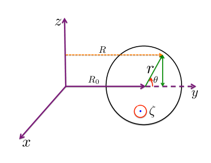
Figure 1: Schematic diagram of the coordinates of a concentric cross section tokamak.

$$\vec{E}=-\nabla\phi=-\biggl{[}\frac{\partial\phi}{\partial\psi}\nabla\psi+\frac{\partial\phi}{\partial\theta}\nabla\theta+\frac{\partial\phi}{\partial\zeta}\nabla\zeta\biggr{]},$$ (6)

where

$$v^{\psi}=\dot{\psi},\quad v^{\theta}=\dot{\theta},\quad v^{\zeta}=\dot{\zeta}r\text{cos}\theta/(R_{0}+r\text{cos}\theta),$$

$$\vec{e}_{\psi}=[\text{cos}\theta\text{cos}\zeta\hat{x}-\text{cos}\theta\text{sin}\zeta\hat{y}+\text{sin}\theta\hat{z}](\partial r/\partial\psi),$$

$$\vec{e}_{\theta}=-r\text{sin}\theta\text{cos}\zeta\hat{x}+r\text{sin}\theta\text{sin}\zeta\hat{y}+r\text{cos}\theta\hat{z},$$ (7)

$$\vec{e}_{\zeta}=-(R_{0}+r\text{cos}\theta)\text{sin}\zeta\hat{x}-(R_{0}+r\text{cos}\theta)\text{cos}\zeta\hat{y}$$

$$\psi(r)=\int_{0}^{r}(r/q)dr\quad\quad\quad\quad\quad\quad\quad\quad$$

Ion dynamics - Ion dynamics is described by the six dimensional Vlasov equation,

$$\biggl{[}\frac{\partial}{\partial t}+\vec{v}\cdot\nabla+\frac{Z_{i}}{m_{i}}(\vec{E}+\vec{v}\times\vec{B})\cdot\frac{\partial}{\partial\vec{v}}\biggr{]}f_{i}=0,$$ (8)

where $f_{i}$ is the ion distribution function, $Z_{i}$ is the ion charge, and $m_{i}$ is the ion mass.

The evolution of the ion distribution function $f_{i}$ can be described by the Newtonian equation of motion in the presence of self-consistent electromagnetic field as follows

$$\frac{d}{dt}\vec{r}=\vec{v},\quad\quad\frac{d}{dt}\vec{v}=\frac{Z_{i}}{m_{i}}\biggl{[}\vec{E}+\vec{v}\times\vec{B}\biggr{]}$$ (9)

In our simulation we compute the marker particle trajectory [Eq.(9)] by the time centered Boris push methodBoris (1970); Birdsall and Langdon (2005); Kuley et al. (2013) as discussed in the following section.

In our GTC simulation we have implemented both perturbative $(\delta f)$ and non-perturbative (full-$f$) methods. We use $(\delta f_{i})$ method to reduce the particle noise. Now we decompose the distribution function $(f_{i})$ into its equilibrium $(f_{0i})$ and perturb part $(\delta f_{i})$ i.e., $f_{i}=f_{0i}+\delta f_{i}$. The perturbed density for ion is defined as the fluid moment of ion distribution function, $\delta n_{i}=\int\delta f_{i}d^{3}v$. By defining the particle weight $w_{i}=\delta f_{i}/f_{i}$, we can rewrite the Vlasov equation for Maxwellian ion with uniform temperature $T_{i}$ and uniform density as follows

$$\frac{d}{dt}w_{i}=-\frac{Z_{i}}{T_{i}}(1-w_{i})\biggl{[}\frac{\partial\phi}{\partial\psi}v^{\psi}+\frac{\partial\phi}{\partial\theta}v^{\theta}+\frac{\partial\phi}{\partial\zeta}v^{\zeta}\biggr{]}$$ (10)

Electron dynamics - Electron dynamics is described by the five-dimensional drift kinetic equation

$$\biggl{[}\frac{\partial}{\partial t}+\dot{\vec{X}}\cdot\nabla+\dot{v}_{\parallel}\frac{\partial}{\partial v_{\parallel}}\biggr{]}f_{e}(\vec{X},v_{\parallel},\mu,t)=0$$ (11)

where $f_{e}$ is the guiding center distribution function, $\vec{X}(\psi,\theta,\zeta)$ is the guiding center position, $\mu$ is the magnetic moment, and $v_{\parallel}$ is the parallel velocity. The evolution of the electron distribution function can be described by the following equations of guiding center motion:Brizard and Hahm (2007)

$$\dot{\vec{X}}=v_{\parallel}\hat{b}+\vec{v}_{E}+\vec{v}_{c}+\vec{v}_{g},$$

$$\dot{v}_{\parallel}=-\frac{1}{m_{e}}\frac{\vec{B}^{*}}{B}\cdot(\mu\nabla B-e\nabla\phi),$$ (12)

where $\vec{B}^{*}=\vec{B}+Bv_{\parallel}/\omega_{ce}\nabla\times\hat{b}$, and $\mu=m_{e}v_{\perp}^{2}/2B$. The $\vec{E}\times\vec{B}$ drift velocity $\vec{v}_{E}$, the grad-$B$ drift velocity $\vec{v}_{g}$, and curvature drift velocity $\vec{v}_{c}$ are given by

$$\vec{v}_{E}=\frac{c\hat{b}\times\nabla\phi}{B},$$

$$\vec{v}_{g}=\frac{\mu}{m\omega_{ce}}\hat{b}\times\nabla B,$$ (13)

$$\vec{v}_{c}=\frac{v_{\parallel}^{2}}{\omega_{ce}}\nabla\times\hat{b}.$$

This electron model is suitable for the dynamics with the wave frequency $\omega\ll\omega_{ce}$ and $k_{\perp}\rho_{e}\ll 1$, where $\omega_{ce}$ is the electron cyclotron frequency and $\rho_{e}$ is the electron gyro radius. Electron dynamics are described by conventional Runge-Kutta method. The perturbed density for electron also can be found from the fluid moment of electron distribution function, $\delta n_{e}=\int\delta f_{e}d^{3}v$. The weight equation for electron can be written as

$$\frac{d}{dt}w_{e}=(1-w_{e})\biggl{[}-e\frac{\vec{B}^{*}}{B_{0}}\cdot\nabla\phi\frac{1}{m_{e}}\frac{1}{f_{0e}}\frac{\partial f_{0e}}{\partial v_{\parallel}}\biggr{]}$$ (14)

where $w_{e}=\delta f_{e}/f_{e}$ and $f_{e}=f_{0e}+\delta f_{e}$. $f_{0e}$ and $\delta f_{e}$ are the equilibrium and perturbed distribution function, respectively. Simulation related to nonuniform plasma density and temperature will be reported in future work.

Field equation - This paper describes the electrostatic model of fully kinetic ion and drift kinetic electron. Most recently Bao et al. have formulated the electromagnetic description of this model.Bao et al. (2015a) The electrostatic potential can be calculated from the Poisson’s equation

$$\nabla_{\perp}\cdot\biggl{[}\biggl{(}1+\frac{\omega_{p}^{2}}{\omega_{c}^{2}}\biggr{)}\nabla_{\perp}\phi\biggr{]}=-4\pi(Z_{i}\delta n_{i}-e\delta n_{e})$$ (15)

Here we consider that fact that the perpendicular wavelength is much shorter than the parallel wavelength to suppress the high frequency electron plasma oscillation along the magnetic field line. Second term on the left hand side corresponds to the electron density due to its perpendicular polarization drift. For an axisymmetric system, the perpendicular Laplacian can be explicitly expressed asXiao et al. (2015)

$$\nabla_{\perp}^{2}=\text{g}^{\psi\psi}\frac{\partial^{2}}{\partial\psi^{2}}+2\text{g}^{\psi\theta}\frac{\partial^{2}}{\partial\psi\partial\theta_{0}}+(\text{g}^{\theta\theta}+\text{g}^{\zeta\zeta}/q^{2})\frac{\partial^{2}}{\partial\theta_{0}^{2}}$$

$$+\frac{1}{J}\biggl{(}\frac{\partial J\text{g}^{\psi\psi}}{\partial\psi}+\frac{\partial J\text{g}^{\psi\theta}}{\partial\theta_{0}}\biggr{)}\frac{\partial}{\partial\psi}+\frac{1}{J}\biggl{(}\frac{\partial J\text{g}^{\psi\theta}}{\partial\psi}+\frac{\partial J\text{g}^{\theta\theta}}{\partial\theta_{0}}\biggr{)}\frac{\partial}{\partial\theta_{0}}$$

where $\theta_{0}=\theta-\zeta/q$, and $\zeta_{0}=\zeta$. In GTC we used the field aligned coordinates $(\psi,\theta_{0},\zeta_{0})$, for reducing the number of parallel grids. Secondly we use the B-spline representation of the magnetic field, which provides a transformation $R=R(\psi,\theta)$, and $Z=Z(\psi,\theta)$, where $(R,Z,\zeta)$ are the cylindrical coordinates. We define the contravariant geometric tensor $\text{g}^{\xi^{\alpha}\xi^{\beta}}=\nabla{\xi^{\alpha}}\cdot\nabla{\xi^{\beta}}$, $(\xi^{1},\xi^{2},\xi^{3})=(\psi,\theta,\zeta)$. The covariant geometric tensor $\text{g}_{\xi^{\alpha}\xi^{\beta}}$ can be expressed as

$$\text{g}_{\psi\psi}=\biggl{(}\frac{\partial R}{\partial\psi}\biggr{)}^{2}+\biggl{(}\frac{\partial Z}{\partial\psi}\biggr{)}^{2},$$

$$\text{g}_{\theta\theta}=\biggl{(}\frac{\partial R}{\partial\theta}\biggr{)}^{2}+\biggl{(}\frac{\partial Z}{\partial\theta}\biggr{)}^{2},$$ (17)

$$\text{g}_{\psi\theta}=\frac{\partial R}{\partial\psi}\frac{\partial R}{\partial\theta}+\frac{\partial Z}{\partial\psi}\frac{\partial Z}{\partial\theta},$$

and $\text{g}_{\psi\theta}=\text{g}_{\theta\psi},\text{g}_{\zeta\zeta}=R^{2}=(R_{0}+r\text{cos}\theta)^{2}$ for concentric cross-section tokamak, where $R_{0}$ is the major radius of the tokamak.

II.2 Boris push for ion dynamics

The efficiency of particle simulation strongly depends on the particle pusher. Boris scheme is the most widely used orbit integrator in explicit particle-in-cell (PIC) simulation of plasmas. In this paper we have extended our Boris push scheme from cylindrical geometry to toroidal geometry.Kuley et al. (2013) This scheme offers second order accuracy while requiring only one force (or field) evaluation per step. The interplay between the PIC cycle and the Boris scheme is schematically represented in Fig.2. At the beginning of each cycle the position of the particles and their time centered velocity $\vec{v}(t-1/2)$, weight $w_{i}(t)$, as well as the grid based electromagnetic fields $\vec{E}(t),\vec{B}(t)$ are given.

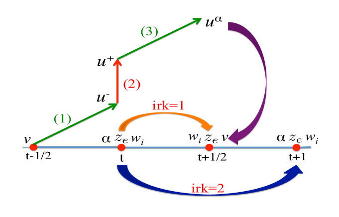
Figure 2: Schematic diagram for the PIC cycle and ion Boris push. The first step indicates the addition of the first half of the electric field acceleration to the velocity $(v\rightarrow u^{-})$. The second step is rotation of the velocity vector $(u^{-}\rightarrow u^{+})$. In the third step, we add the second half of the electric field impulse to the rotated velocity component $(u^{+}\rightarrow u^{\alpha},\alpha=\psi,\theta,\zeta)$. Ion particle weight $(w_{i})$ and electron guiding center $(z_{e})$ are updated using the second order Runge-Kutta (irk=1 and irk=2) method. Dark purple blue indicates the transformation from $u^{\alpha}\rightarrow v$, which is needed to update the ion position [cf. Eq.(27)].

In the first step, we add the first half of the electric field acceleration to the velocity $\vec{v}(t-1/2)$ to obtain the velocity at the particle position $\vec{r}(t)$ as follows

$$\vec{u}(t)=\vec{v}(t-1/2)+\frac{Z_{i}}{m_{i}}\frac{\Delta t}{2}\vec{E}(t)$$ (18)

One can write down the components of velocity at particle position $\vec{r}(t)$ as

$$u^{\alpha-}(t)=\sum_{\beta=\psi,\theta,\zeta}v^{\beta}(t-1/2)\vec{e}_{\beta}(t-1/2)\cdot\nabla\alpha(t)$$

$$+\frac{Z_{i}}{m_{i}}\frac{\Delta t}{2}\vec{E}(t)\cdot\nabla\alpha(t)$$ (19)

where $\alpha=\psi,\theta,\zeta$. We note that in Boozer coordinates, the basis vectors are non-orthogonal in nature. However, for simplicity we consider the orthogonal components only, and Eq.(19) can be rewrite as follows

$$u^{\psi-}(t)=\frac{1}{\text{g}_{\psi\psi}(t)}\biggl{[}v^{\psi}(t-1/2)\vec{e}_{\psi}(t-1/2)\cdot\vec{e}_{\psi}(t)\quad\quad\quad\quad$$

$$+v^{\theta}(t-1/2)\vec{e}_{\theta}(t-1/2)\cdot\vec{e}_{\psi}(t)\quad\quad\quad\quad$$

$$+v^{\zeta}(t-1/2)\vec{e}_{\zeta}(t-1/2)\cdot\vec{e}_{\psi}(t)\biggr{]}+\frac{Z_{i}}{m_{i}}\frac{\Delta t}{2}\vec{E}(t)\cdot\nabla\psi(t),$$

$$u^{\theta-}(t)=\frac{1}{\text{g}_{\theta\theta}(t)}\biggl{[}v^{\psi}(t-1/2)\vec{e}_{\psi}(t-1/2)\cdot\vec{e}_{\theta}(t)\quad\quad\quad\quad$$

$$+v^{\theta}(t-1/2)\vec{e}_{\theta}(t-1/2)\cdot\vec{e}_{\theta}(t)\quad\quad\quad\quad$$

$$+v^{\zeta}(t-1/2)\vec{e}_{\zeta}(t-1/2)\cdot\vec{e}_{\theta}(t)\biggr{]}+\frac{Z_{i}}{m_{i}}\frac{\Delta t}{2}\vec{E}(t)\cdot\nabla\theta(t),$$

$$u^{\zeta-}(t)=\frac{1}{\text{g}_{\zeta\zeta}(t)}\biggl{[}v^{\psi}(t-1/2)\vec{e}_{\psi}(t-1/2)\cdot\vec{e}_{\zeta}(t)\quad\quad\quad\quad$$

$$+v^{\theta}(t-1/2)\vec{e}_{\theta}(t-1/2)\cdot\vec{e}_{\zeta}(t)\quad\quad\quad\quad$$

$$+v^{\zeta}(t-1/2)\vec{e}_{\zeta}(t-1/2)\cdot\vec{e}_{\zeta}(t)\biggr{]}+\frac{Z_{i}}{m_{i}}\frac{\Delta t}{2}\vec{E}(t)\cdot\nabla\zeta(t)$$

Using Eq.(7) we can simplify the above equations as

$$u^{\psi-}(t)=\frac{(\partial r/\partial\psi)_{t}}{\text{g}_{\psi\psi}(t)}\biggl{[}Av^{\psi}(t-1/2)(\partial r/\partial\psi)_{t-1/2}\quad\quad$$

$$+Bv^{\theta}(t-1/2)r(t-1/2)\quad\quad\quad$$

$$+Cv^{\zeta}(t-1/2)(R_{0}+r(t-1/2)\text{cos}\theta(t-1/2))\biggr{]}$$

$$-\frac{Z_{i}}{m_{i}}\frac{\Delta t}{2}\frac{\partial\phi}{\partial\psi}\text{g}^{\psi\psi},$$

$$u^{\theta-}(t)=\frac{1}{\text{g}_{\theta\theta}(t)}\biggl{[}Dv^{\psi}(t-1/2)(\partial r/\partial\psi)_{t-1/2}r(t)\quad\quad$$

$$+Ev^{\theta}(t-1/2)r(t-1/2)r(t)\quad\quad\quad$$

$$+Fv^{\zeta}(t-1/2)r(t)(R_{0}+r(t-1/2)\text{cos}\theta(t-1/2))\biggr{]}$$

$$-\frac{Z_{i}}{m_{i}}\frac{\Delta t}{2}\frac{\partial\phi}{\partial\theta}\text{g}^{\theta\theta},$$

$$u^{\zeta-}(t)=\frac{1}{\text{g}_{\zeta\zeta}(t)}\biggl{[}Gv^{\psi}(t-1/2)(\partial r/\partial\psi)_{t-1/2}\quad\quad\quad\quad$$

$$+Hv^{\theta}(t-1/2)r(t-1/2)\quad\quad\quad\quad$$

$$+Pv^{\zeta}(t-1/2)(R_{0}+r(t-1/2)\text{cos}\theta(t-1/2))\biggr{]}$$

$$\times(R_{0}+r(t)\text{cos}\theta(t))-\frac{Z_{i}}{m_{i}}\frac{\Delta t}{2}\frac{\partial\phi}{\partial\zeta}\text{g}^{\zeta\zeta},\quad\quad$$ (21)

where

$$A=P\text{cos}\theta_{1}\text{cos}\theta_{2}+\text{sin}\theta_{1}\text{sin}\theta_{2},$$

$$B=-P\text{sin}\theta_{1}\text{cos}\theta_{2}+\text{cos}\theta_{1}\text{sin}\theta_{2},$$

$$C=\text{cos}\theta_{2}(-\text{sin}\zeta_{1}\text{cos}\zeta_{2}+\text{cos}\zeta_{1}\text{sin}\zeta_{2}),$$

$$D=-P\text{cos}\theta_{1}\text{sin}\theta_{2}+\text{sin}\theta_{1}\text{cos}\theta_{2},$$

$$E=P\text{sin}\theta_{1}\text{sin}\theta_{2}+\text{cos}\theta_{1}\text{cos}\theta_{2},$$ (22)

$$F=\text{sin}\theta_{2}(\text{sin}\zeta_{1}\text{cos}\zeta_{2}-\text{cos}\zeta_{1}\text{sin}\zeta_{2}),$$

$$G=\text{cos}\theta_{1}(-\text{cos}\zeta_{1}\text{sin}\zeta_{2}+\text{sin}\zeta_{1}\text{cos}\zeta_{2}),$$

$$P=\text{cos}\zeta_{1}\text{cos}\zeta_{2}+\text{sin}\zeta_{1}\text{sin}\zeta_{2}$$

$$H=-G\text{tan}\theta_{1},\theta_{1}=\theta(t-1/2),\theta_{2}=\theta(t)$$

$$\zeta_{1}=\zeta(t-1/2),\zeta_{2}=\zeta(t)$$

In the second step we consider the rotation of the velocity at time $(t)$. Rotated vector can be written as

$$\vec{u}^{+}(t)=\vec{u}^{-}(t)+\vec{u}^{-}(t)\times\vec{s}(t)+[\vec{u}^{-}(t)\times\vec{T}(t)]\times\vec{s}(t)$$ (23)

where $\vec{T}=(Z_{i}\vec{B}/m_{i})(\Delta t/2)$ and $\vec{s}=2\vec{T}/(1+T^{2})$. Most recently Wei et al.,Wei et al. (2015) have developed the single particle ion dynamics in general geometry using both toroidal and poloidal components of magnetic field. In our formulations we also incorporate both toroidal and poloidal components of magnetic field. However, for simplicity during rotation we consider the toroidal component of magnetic field only, $\vec{B}=g\nabla\zeta=q\nabla\psi\times\nabla\theta$, and the components of the rotated vector become

$$u^{\psi+}(t)=\biggl{[}1-\biggl{(}\frac{2}{1+T^{2}}\biggr{)}\biggr{(}\frac{Z_{i}}{m_{i}}\frac{\Delta t}{2}\biggr{)}^{2}B^{2}\biggr{]}u^{\psi-}(t)$$

$$+\biggl{(}\frac{2}{1+T^{2}}\biggr{)}\biggr{(}\frac{Z_{i}}{m_{i}}\frac{\Delta t}{2}\biggr{)}\biggl{(}\frac{g}{J}\biggr{)}\text{g}_{\theta\theta}(t)u^{\theta-}(t),$$

$$u^{\theta+}(t)=\biggl{[}1-\biggl{(}\frac{2}{1+T^{2}}\biggr{)}\biggr{(}\frac{Z_{i}}{m_{i}}\frac{\Delta t}{2}\biggr{)}^{2}B^{2}\biggr{]}u^{\theta-}(t)$$

$$-\biggl{(}\frac{2}{1+T^{2}}\biggr{)}\biggr{(}\frac{Z_{i}}{m_{i}}\frac{\Delta t}{2}\biggr{)}\biggl{(}\frac{g}{J}\biggr{)}\text{g}_{\psi\psi}(t)u^{\psi-}(t),$$ (24)

$$u^{\zeta+}(t)=u^{\zeta-}(t)\quad\quad\quad\quad\quad\quad\quad\quad\quad\quad\quad\quad\quad$$

where $T=(Z_{i}B/m_{i})(\Delta t/2)$. We assume orthogonal basis vectors, so the off-diagonal terms of metric tensor are zero, and one can redefine the Jacobian as $J^{2}=\text{g}_{\psi\psi}\text{g}_{\theta\theta}\text{g}_{\zeta\zeta}$, and the diagonal components of the metric tensor as $\text{g}_{\psi\psi}=(\partial r/\partial\psi)^{2}$, $\text{g}_{\theta\theta}=r^{2}$, $\text{g}_{\zeta\zeta}=(R_{0}+r\text{cos}\theta)^{2}$. For $g=1$, and $B=(1+r/R_{0}\text{cos}\theta)^{-1}$, one can explicitly prove that

$${u^{\psi+}}^{2}\text{g}_{\psi\psi}(t)+{u^{\theta+}}^{2}\text{g}_{\theta\theta}(t)+{u^{\zeta+}}^{2}\text{g}_{\zeta\zeta}(t)=$$

$${u^{\psi-}}^{2}\text{g}_{\psi\psi}(t)+{u^{\theta-}}^{2}\text{g}_{\theta\theta}(t)+{u^{\zeta-}}^{2}\text{g}_{\zeta\zeta}(t)$$ (25)

i.e., the magnitude of velocity is unchanged during the rotation. In the third step, we add the other half electric acceleration to the rotated vectors to obtain the velocity at time $(t+1/2)$

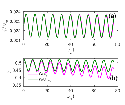
Figure 3: Verification of $\vec{E}\times\vec{B}$ drift in toroidal geometry. Time variations of (a) poloidal flux function and (b) poloidal angle of the ion position. Here $\psi_{w}$ is the poloidal flux function at the last closed flux surface.

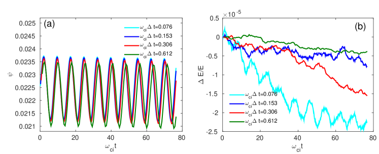
Figure 4: Time step convergence of (a) poloidal flux function, and (b) relative energy error of ion.

$$u^{\alpha}(t+1/2)=u^{\alpha+}(t)+\frac{Z_{i}}{m_{i}}\frac{\Delta t}{2}\vec{E}(t)\cdot\nabla\alpha(t)$$ (26)

To update the particle position we need to recover $\vec{v}(t+1/2)$, which can be done through the following transformation (cf. Fig.2 dark purple arrow)

$$v^{\gamma}(t+1/2)=\sum_{\alpha=\psi,\theta,\zeta}u^{\alpha}(t+1/2)\vec{e}_{\alpha}(t)\cdot\nabla\gamma(t+1/2)$$ (27)

where $\gamma=\psi,\theta,\zeta$. However, the basis vector $\nabla\gamma(t+1/2)$ is still unknown, since $\gamma(t+1/2)$ does not exist in standard leap-frog scheme. Here we use an estimator for $\gamma(t+1/2)$ as

$$\gamma(t+1/2)=\gamma(t)+u^{\gamma}(t+1/2)\frac{\Delta t}{2}$$ (28)

After we find the velocity at time $(t+1/2)$, we can update the particle position using the leap-frog scheme as

$$\gamma(t+1)=\gamma(t)+v^{\gamma}(t+1/2)\Delta t$$ (29)

In Eq.(27) we have the dot-product of two basis vectors at different time steps. We have evaluated this equation in the similar way as described in Eqs. (20)-(22).

To verify this cyclotron integrator we have carried out a single particle ion dynamics in toroidal geometry with inverse aspect ratio $r/R_{0}=0.357$, and $\rho_{i}/r=0.0048$. First we calculate the time variations of the the poloidal flux function and the poloidal angle in the absence of electric field [cf. Fig.3 green line]. Secondly we introduce a radial electric field in the particle equation of motion. In the presence of this static electric field, an ion will experience a $\vec{E}\times\vec{B}$ drift in the poloidal direction, as shown in Fig.3 (magenta line). These results between the theory and GTC simulations are summarized in Table I.

Fig. 4(a)-(b) show the time step convergence of the poloidal flux function and the relative energy error of the marker particle. Fig. 4(a) shows that poloidal flux function can converge with 40 time steps per cyclotron period $(\omega_{ci}\Delta t=0.153)$. However, there is no such time dependent relation for the calculation of the energy error. Error in the energy arises mostly due to the decomposition of velocity during first and last steps of the Boris scheme and it is in the acceptable limit $(\sim 10^{-5})$.

In the above section we have discussed the time advancement of the dynamical quantities like velocity and position of ion in the time centered manner. However, for the the self-consistent simulation we need to update particle weight, electron guiding center and electric field. We use the second order Runge-Kutta (RK) method, to advance these quantities, which can be described as follows. In our global simulation we use reflective boundary condition for the particle and fields.

II.3 RK pusher for particle weight and electron dynamics

Using the initial ion velocity at time $(t-1/2),$ the ion particle push module update the velocity up to (t+1/2). The velocity at time (t) is computed by linear average of velocities as follows

$$v^{\gamma}(t)=\frac{v^{\gamma}(t-1/2)+v^{\gamma}(t+1/2)}{2}$$ (30)

Now using the electric field and average velocity at time $(t)$, one can compute $(dw_{i}/dt)$ from Eq.(10). For the first step of the RK method we advance the particle weight from $w_{i}(t)$ to $w_{i}(t+1/2)$, and $w_{e}(t)$ to $w_{e}(t+1/2)$. With the updated values of the source term (charge density), the field solver compute the electric field at time $(t+1/2)$ (cf. Fig.2 orange arrow). In the second step of RK we use the updated electric field at $(t+1/2)$ for the advancement of the particle weight, and electron guiding center $(z_{e})$ from $(t)$ to $(t+1)$ [cf. Fig.2 dark blue arrow]. Mathematically we can write these two steps as follows

• First step (irk=1)

$$\blacktriangleright\text{Ion pusher}\rightarrow w_{i}(t+1/2)=w_{i}(t)+\frac{dw_{i}}{dt}\biggr{|}_{t}\frac{\Delta t}{2},\quad\quad\quad$$

$$\left.\begin{aligned} \blacktriangleright\text{Electron}&\\ \text{pusher}&\end{aligned}\right.\quad\Rightarrow\left\{\begin{aligned} &z_{e}(t+1/2)=z_{e}(t)+\frac{dz_{e}}{dt}\biggr{|}_{t}\frac{\Delta t}{2}\\ &w_{e}(t+1/2)=w_{e}(t)+\frac{dw_{e}}{dt}\biggr{|}_{t}\frac{\Delta t}{2}\quad\quad\end{aligned}\right.$$

$$\bullet\quad\text{Solve field solver for}\quad\vec{E}(t+1/2)\quad\quad\quad\quad\quad\quad\quad\quad\quad$$

• Second step (irk=2)

$$\blacktriangleright\text{Ion pusher}\rightarrow w_{i}(t+1)=w_{i}(t)+\frac{dw_{i}}{dt}\biggr{|}_{(t+1/2)}\Delta t,\quad\quad\quad$$

$$\left.\begin{aligned} \blacktriangleright\text{Electron}&\\ \text{pusher}&\end{aligned}\right.\Rightarrow\left\{\begin{aligned} &z_{e}(t+1)=z_{e}(t)+\frac{dz_{e}}{dt}\biggr{|}_{(t+1/2)}\Delta t\\ &w_{e}(t+1)=w_{e}(t)+\frac{dw_{e}}{dt}\biggr{|}_{(t+1/2)}\Delta t\quad\quad\end{aligned}\right.$$

$$\bullet\quad\text{Solve field solver for}\quad\vec{E}(t+1)\quad\quad\quad\quad\quad\quad\quad\quad\quad\quad$$

Table 1: Comparison of ion cyclotron motion including $\vec{E}\times\vec{B}$ drift from simulation and theory

Parameter	Theory	GTC Simulation
Gyro radius	8.415$\times 10^{-3}$(m)	8.46$\times 10^{-3}$(m)
Gyro frequency	4.557$\times 10^{6}$(rad/sec)	4.538$\times 10^{6}$(rad/sec)
$\vec{E}\times\vec{B}$ drift	1.815$\times 10^{4}$(m/s)	1.785$\times 10^{4}$(m/s)

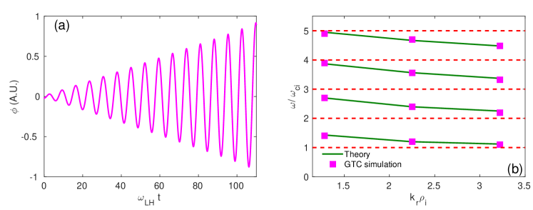
Figure 5: Verification of Normal modes in toroidal geometry. (a) Time history of LH wave amplitude excited by antenna, (b) comparison of IBW dispersion relation between the analytical solution and the GTC simulations for the first four harmonics.

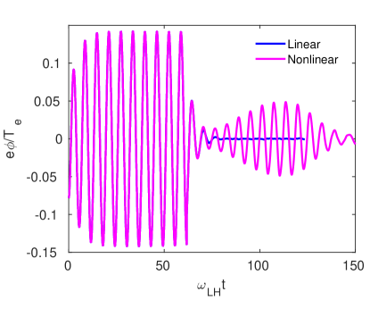
Figure 6: Nonlinear GTC simulation of LH wave exhibits oscillation in wave amplitude (magenta line), while linear simulation shows exponential decay (blue line).

III Linear Verification of Normal modes and nonlinear particle trapping

In this section, we will discuss the electrostatic normal modes with $k_{\parallel}=0$ as a benchmark of toroidal Boris scheme in the linear simulation. The general dispersion relation of the normal mode in uniform plasma can be written as Liu and Tripathi (1986)

$$1+\chi_{j}=0$$ (31)

For a Maxwellian background, one can write down the susceptibility as

$$\chi_{j}=-\sum_{j=e,i}\frac{1}{k^{2}\lambda_{Dj}^{2}}\sum_{l=1}^{\infty}\frac{2l^{2}\omega_{cj}^{2}}{\omega^{2}-l^{2}\omega_{cj}^{2}}I_{l}(b_{j})e^{-b_{j}}$$ (32)

where $b_{j}=k_{\perp}^{2}\rho_{j}^{2}$, $\rho_{j}=\sqrt{(T_{j}/m_{j})}/\omega_{cj}$, $\lambda_{Dj}^{2}=\epsilon_{0}T_{j}/n_{0j}e^{2}$, and $\omega_{ci}=Z_{i}B/m_{i}$. For normal modes (LHW, IBW), we have $|\omega/\omega_{ce}|\sim\mathcal{O}(\omega/\omega_{ce})\ll 1$ and $k_{\perp}\rho_{e}\ll 1$, hence the electron susceptibility is dominated by $l=1$ term. So the above Eq (32) becomes

$$1+\frac{\omega_{pe}^{2}}{\omega_{ce}^{2}}-\frac{1}{k_{\perp}^{2}\lambda_{Di}^{2}}\sum_{l=1}^{\infty}\frac{2l^{2}\omega_{ci}^{2}}{\omega^{2}-l^{2}\omega_{ci}^{2}}I_{l}(b_{i})e^{-bi}=0$$ (33)

For long wavelength limit $k\rightarrow 0^{+}$, with $\omega_{ci}\ll\omega\ll\omega_{ce}$, the frequency of the LH is

$$\omega_{LH}^{2}=\omega_{pi}^{2}\biggl{(}1+\frac{\omega_{p}^{2}}{\omega_{c}^{2}}\biggr{)}^{-1}$$ (34)

We use an artificial antenna to excite these modes and to verify the mode structure and frequency in our simulation. The electrostatic potential of the antenna can be written as:

$$\phi_{ext}=\phi_{0}\text{sin}(k_{r}r)\text{cos}(\omega_{0}t)\text{cos}(m_{0}\theta-n_{0}\zeta)$$ (35)

In our simulation, the inverse aspect ratio of the tokamak is $r/R_{0}=0.018$, $\rho_{i}/r=0.002$, and the background plasma density is uniform with a uniform temperature. We use poloidal and toroidal mode filters to select m=0, n=0 modes. For the lower hybrid simulation, $\omega_{pi}=145.2\omega_{ci}$,, $\omega_{pe}=6242.8\omega_{ci}$, $\omega_{ci}\Delta t\simeq 1.33\times 10^{-3}$, $m_{e}/m_{i}=5.44618\times 10^{-4}$, and particles per wavelength are $8\times 10^{6}$. We carry out the scan with different antenna frequencies, and find out the frequency in which the mode response has the maximum growth of the amplitude. That frequency is then identified as the eigenmode frequency of the system. Fig. 5(a) shows the time history of the lower hybrid wave amplitude for the antenna frequency $\omega_{0}=41.0\omega_{ci}$, which agrees well with the analytical frequency $40.9\omega_{ci}$. Also the amplitude of the LH wave increases linearly with time, since there is no damping due to $k_{\parallel}=0$. To avoid the boundary effects we consider $(\Delta/\rho_{i}=41.13)$, where $\Delta$ is the width of the simulation domain.

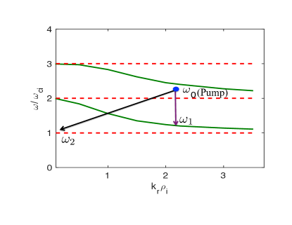
Figure 7: Schematic of an IBW parametric decay process. Pump wave $(\omega_{0},\vec{k}_{0})$ decays into an IBW side band $(\omega_{1},\vec{k}_{1})$ and an ion cyclotron quasi mode (ICQM) $(\omega_{2},\vec{k}_{2})$. Green lines represent the theoretical dispersion curve of the IBW for first two harmonics.

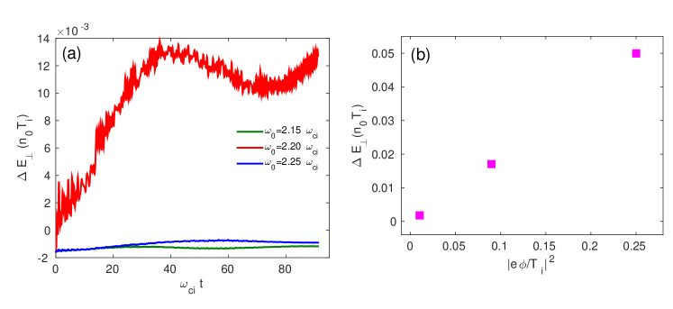
Figure 8: (a) Time history of change of perpendicular kinetic energy of ion for different pump wave frequency, and (b) change in kinetic energy of ion as a function of intensity of the pump wave.

Similarly we carried out the simulation of the IBW waves for the first four harmonics $(l=1-4)$. In this simulation by changing the plasma density we consider $\omega_{pi}=10.01\omega_{ci}$, $\omega_{pe}=422.3\omega_{ci}$, $\Delta/\rho_{i}=19.45$, $\omega_{ci}\Delta t\simeq 0.055$, and particles per wavelength are $8\times 10^{6}$. Fig. 5(b) shows a good agreement between the analytical and GTC simulation results of the IBW frequency.

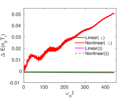
Figure 9: Time history of change of kinetic energy of ion. Green and magenta lines represent the energy change during linear simulation in the perpendicular and parallel direction, respectively. Red and dotted lines indicate the energy change during nonlinear simulation in the perpendicular and parallel direction, respectively.

As a first step in developing this nonlinear toroidal particle simulation model, we carry out the nonlinear GTC simulation of electron trapping by the LH wave with a large amplitude [cf. Fig. 6] in cylindrical geometry. Initially the linear lower hybrid eigen mode $(m=4$, and $n=1)$ is excited using an artificial antenna. After the wave amplitude reaches the plateau regime, we turn off the antenna, and the wave decays exponentially due to the Landau damping on electrons in the linear simulation (blue line).Bao et al. (2014) The linear damping rates obtained from the theory $(0.3\omega_{LH})$ agree well with the simulation $(0.31\omega_{LH})$. However, in the nonlinear simulation, the resonant electrons can be trapped by the electric field of the wave. The wave amplitude become oscillatory with a frequency equal to the trapped electron oscillation frequency (magenta line). The bounce frequencies $\omega_{b}=k_{\parallel}v_{the}\sqrt{e\phi/T_{e}}$ are close to the analytical values (Table II). During the antenna excitation of LH wave eignemode, the particle dynamics are linear for both linear and nonlinear simulation.

Table 2: Comparison of bounce frequency of nonlinearly trapped particle in LH wave simulation

$e\phi/T_{e}$	Theory	GTC Simulation
0.00885	2.91$\omega_{ci}$	3.04$\omega_{ci}$
0.04866	6.8$\omega_{ci}$	6.7$\omega_{ci}$

IV PDI of ion cyclotron wave and Nonlinear Ion heating

Magnetized plasma supports a large number of electrostatic and electromagnetic modes. When wave energy is still relatively low, these modes are mutually independent and represent a description for the response of the plasma to local perturbation and external field. However, at higher amplitudes these modes are coupled and exchange momentum and energy with each other through the coherent wave phenomenon , e.g., parametric decay instabilities (PDI). In this process the pump wave $(\omega_{0},\vec{k}_{0})$ decays into two daughter waves or one daughter wave $(\omega_{1},\vec{k}_{1})$ and a quasimode $(\omega_{2},\vec{k}_{2})$ pair. The selection rule for this decay process is given by

$$\omega_{0}=\omega_{1}+\omega_{2}\quad\quad\quad\vec{k}_{0}=\vec{k}_{1}+\vec{k}_{2}$$ (36)

Looking at Figure 7, we see that in this case, the pump wave can decay into one daughter with a near zero wavenumber and another wave with nearly the same wavenumber as the pump wave. This process is considered to be the most probable non-resonant decay channel of PDI in the ion cyclotron heating regime. Possible decay channels in the ion cyclotron range of frequency in experiments have been discussed by Porkolob.Porkolab (1990) In Figure 7, we show the IBW dispersion relation (green lines) for the same parameter as in Figure 5(b). In our simulation, the pump wave itself is not an IBW, and the value of $\omega/\omega_{ci}$ at the antenna position is 2.25, as indicated in Fig.7. When $\omega_{0}=\omega_{\text{IBW}}+\omega_{ci}$ i.e., the frequency shift of the wave is close to the ion cyclotron frequency, the wave is strongly damped on ions and known as ion cyclotron quasi-mode (ICQM).

In experiment, a pump wave of fixed frequency passing through the nonuniform plasma density and temperature experiences the variation of the wave vector to satisfy the dispersion relation. As a result of this inhomogeneity, layers may exist where selection rules of mode-mode coupling are easily satisfied. However, in our simulation plasma density and temperature are uniform and the wave vectors of the pump wave and the sideband wave are chosen by the antenna. To satisfy the frequency matching condition in our simulation, we scan the pump wave frequencies with fixed wavevector. The energy transfer from the wave to ion (nonlinear ion heating) is maximum, when the frequency selection of parametric decay, $\omega_{1}=\omega_{\text{IBW}}$ and $\omega_{2}=\omega_{ci}$ are satisfied (cf. Fig.8(a) red line). Otherwise the energy transfer is negligible (cf. Fig.8(a) green and blue lines). Our simulations are all electrostatic and we consider only m=0, n=0 mode. We consider $\omega_{pi}=10.01\omega_{ci}$, $\omega_{pe}=422.3\omega_{ci}$, $\Delta/\rho_{i}=19.45$, $100$ radial grid points per wavelength, 200 particles per cell. The simulation time step $(\omega_{ci}\Delta t\simeq 0.02)$ is sufficient to resolve IBW, ion cyclotron wave and pump wave dynamics. In this case the particles trajectory are described by the perturbed electric field in addition to the equilibrium magnetic field [cf. IIA]. Fig.8(b) shows that the temperature of the hot ions increases linearly as the amount of rf power increases, since the kinetic energy of the ion [$(1/2)m_{i}(U/c_{s})^{2}$] is proportial to $(e\phi/T_{i})^{2}$, where $U/c_{s}=k_{0\perp}\rho_{i}(e\phi/T_{i})$ is the normalized ion velocity, and $c_{s}=\sqrt{T_{e}/m_{i}}$ is the ion sound speed. We measure the energy of the ion after 400 ion cyclotron periods. This simulation time is long enough to excite the daughter waves for the prominent PDI phenomenon.

Fig.9 shows that ion heating takes place only in the perpendicular direction. The ion temperature in the parallel direction does not change. Since the wave heating affects predominantly the perpendicular ion distribution, which is consistent with the results observed in the scrape-off layer (SOL) of DIII-D,Pinsker et al. (1993) Alcator-C Mod,Rost, Porkolab, and Boivin (2002) and HT-7Li et al. (2001) experiments during the IBW heating and high harmonic fast waves heating in NSTX.Biewer et al. (2005) This parasitic absorption of the wave energy degrade the performance of ion Bernstein and ion cyclotron harmonics resonance heating. However, our simulations are limited to the core region only. In our nonlinear simulation the ponderomotive effect is absent, since we consider the plasma response in the $r$ direction only. With the present simulation setup, the amount of power transferred to the sideband (IBW) has not been measured directly, but the energy of the quasi-mode is measured from the particle diagnosis. During the linear simulation, wave particle interaction can be possible only through the linear damping, which is negligible compared to the nonresonant damping.

V Discussion

In summary, nonlinear global toroidal particle simulations have been developed using fully kinetic ion and drift kinetic electron to study the electron trapping by LHW and parametric decay process of ion cyclotron range of frequency (ICRF) waves in uniform core plasma. We verify our simulation results with the linear dispersion relation. In the nonlinear simulation of LH wave, we find that the amplitude of the electrostatic potential oscillates with a bounce frequency, which is due to the wave trapping of resonant electrons. We also find the nonlinear anisotropic ion heating due to nonresonant three wave coupling. One must mention here that in tokamak scenario with non-uniform density and temperature, energy density of the wave can begin to approach the thermal energy in the edge. Since, in the edge region the densities and temperatures are factors of $10^{2}$ to $10^{3}$ lower than in the core produce strong ponderomotive effects and parametric decay physics.