Radiative heat transfer between spatially nonlocally responding dielectric objects

Abstract

We calculate numerically the heat transfer rate between a spatially dispersive sphere and a half-space. By utilising Huygens’ principle and the extinction theorem, we derive the necessary reflection coefficients at the sphere and the plate without the need to resort to additional boundary conditions. We find for small distances $d\sim 1$nm a significant modification of the spectral heat transfer rate due to spatial dispersion. As a consequence, the spurious divergencies that occur in spatially local approach are absent.

1 Introduction

In the past decade, the advances in nanooptics and nanophotonics made the fabrication of ever smaller dielectric and metallic objects feasible, whose separation can be controlled down to a few nanometers [1, 2, 3, 4]. The near-field of such nanoscopic objects exhibit strong mode confinement and field enhancement due to the presence of evanescent fields. This results in an increase of heat transfer rates several orders of magnitude larger than the classical far-field limit. These enhancements open up new possibilities in numerous applications including thermal near-field imaging [5], heat-assisted magnetic recording [6], nanopatterning [7], and near-field thermophotovoltaics [8].

It is well known that thermal heat transfer described by black-body radiation is an insufficient description for separation distances smaller than the thermal wavelength $\lambda_{T}$. It strongly underestimates the near-field contribution from photon tunnelling mediated by surface phonon-polaritons in polar dielectrics or (spoof) surface plasmon-polaritons at metal interfaces [9, 10] or doped silicon [11] in the near-IR. A theoretical framework, namely fluctuation electrodynamics, has been developed by Rytov as early as the 1950’s (see, e.g. the textbook [12]). In this theory, electromagnetic radiation is created by either the thermal random motion of charge carries, i.e. fluctuating current densities, or fluctuation dipoles in polar media. In linear response theory, these fluctuations are ultimately linked, via the fluctuation-dissipation theorem, to their respective response functions (e.g. conductivity or dielectric permittivity). In the commonly employed spatially local limit, the near-field heat transfer varies with gap distance $d$ for the respective geometries, as $d^{-2}$ (plate-plate), $d^{-1.5}$ (cylinder–cylinder) and $d^{-1}$ (sphere-plate). These findings agree well with several recent experiments [3, 4, 13, 14, 15].

However, in the spatially local theory the calculated heat transfer rate diverges as soon as the separation of the bodies vanishes, i.e. when $d\rightarrow 0$. Recent works [16, 17, 18, 19] showed that, in order to overcome these divergences, spatial nonlocality (or spatial dispersion) of the dielectric tensor must be taken into account. In addition, spatial dispersion changes the mode structure of surface plasmons and thus the spectral heat transfer rate. In general, spatial nonlocality becomes important whenever the electromagnetc field varies appreciably on a length scale comparable with the intrinsic natural length scales of a medium, e.g. the electron mean free path or interatomic spacings. Well-known effects associated with spatial dispersion are the anomalous skin effect and resonant excitation of longitudinal modes in nanoparticles [20], band-gap photoluminescence and dynamical screening [21].

When considering the transition of electromagnetic waves between two media one usually fits the bulk modes at the interface according Maxwell boundary conditions (MBCs). However, in a spatially dispersive media there exist additional longitudinal and transverse modes by virtue of the dispersion relations

$$k^{2}=k^{2}_{0}\varepsilon_{\bot}(\mathbf{k},\omega),\quad\varepsilon_{\parallel}(\mathbf{k},\omega)=0\>,$$ (1)

where $k_{0}=\omega/c$ is the wave number of free space, $\varepsilon_{\bot}(\mathbf{k},\omega)$ is the transverse dielectric function and $\varepsilon_{\parallel}(\mathbf{k},\omega)$ is the longitudinal dielectric function. At the interface of a medium with free space, these modes have to be match with the free-space modes for which the Maxwell boundary conditions are seemingly insufficient. Pekar [22] and later Hopfield and Thomas [23] provided the missing relations by introducing the ad hoc concept of additional boundary conditions (ABCs). Since then, the applicability of these and other ABCs [24] have been a matter of controversy [25, 26, 27]. A disadvantage of ABCs is that the number ABC’s required to match the modes at the surface depends on the number of supported modes by the media. In addition, the choice of the appropriate ABC depends on the particular system under consideration [28]. However, when applying the extinction theorem together with Huygens’ principle, Maxwell’s boundary conditions are indeed sufficient as they contain all information required to match any number of modes for any spatially dispersive media [29].

In this article, we investigate the heat transfer rate between a sphere and a half-space of different types of spatially dispersive media separated by a vacuum gap. We follow the macroscopic approach of fluctuation electrodynamics in which the sources of thermal radiation are expressed via the fluctuation-dissipation theorem. The boundary value problem is dealt with by virtue of Huygens’ principle and the extinction theorem (HuyEx). In Sec. 2 we apply this principle to the scattering problem at a single plate and compare the obtained reflection coefficients with different ABC approaches. In Sec. 3 we derive the thermal emissivity of a spatially dispersive sphere. We combine these results in Sec. 4 to calculate the net heat transfer in the plate-sphere geometry and we present our numerical results.

2 Extinction theorem and Huygens’ principle

2.1 Source-quantity representation of the electromagnetic field

The evolution of an electromagnetic wave is described by the Helmholtz equation. In the case of a spatially nonlocal medium the relation between the displacement field $\mathbf{D}(\mathbf{r},\omega)$ and the electric field $\mathbf{E}(\mathbf{r},\omega)$ is given by a convolution integral

$$\mathbf{D}(\mathbf{r},\omega)=\int\limits\mathrm{d}^{3}r^{\prime}\>\boldsymbol{\mathcal{\varepsilon}}(\mathbf{r},\mathbf{r}^{\prime},\omega)\cdot\mathbf{E}(\mathbf{r}^{\prime},\omega)$$ (2)

where $\boldsymbol{\mathcal{\varepsilon}}(\mathbf{r},\mathbf{r}^{\prime},\omega)$ is the dielectric permittivity tensor. It depends both on the source position $\mathbf{r}^{\prime}$ at which the field excitation occurs as well as on the observation point $\mathbf{r}$ which in general is different from $\mathbf{r}^{\prime}$. Note that a spatially nonlocal permittivity also partially covers (para-)magnetic media [20]. The propagation of the electromagnetic field is then governed by the Helmholtz equation. For spatially dispersive media it becomes an integrodifferential equation, viz.

$$\nabla\times\nabla\times\mathbf{E}(\mathbf{r},\omega)-\frac{\omega^{2}}{c^{2}}\int\limits\mathrm{d}^{3}r^{\prime}\>\boldsymbol{\mathcal{\varepsilon}}(\mathbf{r},\mathbf{r}^{\prime},\omega)\cdot\mathbf{E}(\mathbf{r}^{\prime},\omega)=i\mu_{0}\omega\mathbf{j}(\mathbf{r},\omega)\>.$$ (3)

The electromagnetic field is driven by the current density $\mathbf{j}(\mathbf{r},\omega)$ which becomes the central quantity in fluctuation electrodynamics as well in electromagnetic field quantisation within the framework of macroscopic quantum electrodynamics [30, 31, 32, 33, 34, 35, 36]. The formal solution of the Helmholtz is then

$$\mathbf{E}(\mathbf{r},\omega)=i\mu_{0}\omega\int\limits_{\mathbb{R}^{3}}\mathrm{d}^{3}r^{\prime}\>{\boldsymbol{\mathcal{G}}}(\mathbf{r},\mathbf{r}^{\prime},\omega)\cdot\mathbf{j}(\mathbf{r}^{\prime},\omega)\;.$$ (4)

The dyadic Green function ${\boldsymbol{\mathcal{G}}}(\mathbf{r},\mathbf{r}^{\prime},\omega)$ is the fundamental solution to the Helmholtz equation (3) and is thus the unique solution to

$$\nabla\times\nabla\times{\boldsymbol{\mathcal{G}}}(\mathbf{r},\mathbf{r}^{\prime},\omega)-\frac{\omega^{2}}{c^{2}}\int\limits\mathrm{d}^{3}s\>\boldsymbol{\mathcal{\varepsilon}}(\mathbf{r},\mathbf{s},\omega)\cdot{\boldsymbol{\mathcal{G}}}(\mathbf{s},\mathbf{r}^{\prime},\omega)={\boldsymbol{\mathcal{I}}}\delta(\mathbf{r}-\mathbf{r}^{\prime})$$ (5)

together with the appropriate boundary conditions at infinity. It describes the propagation of an elementary dipolar excitation from $\mathbf{r}^{\prime}$ to $\mathbf{r}$. The dyadic Green function contains all information about the electromagnetic response as well as the geometries of the dielectric media involved. Due to the linearity of the Helmholtz equation, the dyadic Green function can be decomposed into a bulk part $\boldsymbol{\mathcal{G}}_{\mathrm{i}}(\mathbf{r},\mathbf{r}^{\prime},\omega)$ inside one medium, and a scattering part $\boldsymbol{\mathcal{G}}^{(fs)}(\mathbf{r},\mathbf{r}^{\prime},\omega)$ describing transmission and reflection at interfaces between media as

$$\boldsymbol{\mathcal{G}}^{(fs)}(\mathbf{r},\mathbf{r}^{\prime},\omega)=\boldsymbol{\mathcal{G}}_{\mathrm{i}}(\mathbf{r},\mathbf{r}^{\prime},\omega)\delta_{fs}+\boldsymbol{\mathcal{G}}^{(fs)}(\mathbf{r},\mathbf{r}^{\prime},\omega)\;.$$ (6)

Here, $s$ and $f$ denote the regions of the $s$ource and $f$ield points, respectively. Furthermore, the dyadic Green function is reciprocal $\boldsymbol{\mathcal{G}}(\mathbf{r},\mathbf{r}^{\prime},\omega)=\boldsymbol{\mathcal{G}}^{T}(\mathbf{r}^{\prime},\mathbf{r},\omega)$, and it is analytic in the upper half of the complex $\omega$ plane and obeys the Schwarz reflection principle $\boldsymbol{\mathcal{G}}^{\ast}(\mathbf{r},\mathbf{r}^{\prime},\omega)=\boldsymbol{\mathcal{G}}(\mathbf{r},\mathbf{r}^{\prime},-\omega^{\ast})$.

2.2 The dyadic Green function for spatially dispersive bulk media

In the case of an infinitely extended homogeneous medium, the dielectric permittivity becomes translationally invariant, $\boldsymbol{\mathcal{\varepsilon}}(\mathbf{r},\mathbf{r}^{\prime},\omega)\equiv\boldsymbol{\mathcal{\varepsilon}}(\mathbf{r}-\mathbf{r}^{\prime},\omega)$, but still includes potential anisotropy, absorption, as well as spatial and temporal dispersion. The translational invariance allows one to solve Eq. (5) for the bulk Green tensor $\boldsymbol{\mathcal{G}}(\mathbf{r},\mathbf{r}^{\prime},\omega)$ by Fourier transform techniques. As mentioned above, in a spatially dispersive medium it is impossible to distinguish between (transverse) electric and magnetic responses. This allows to gauge all electromagnetic responses into a single dielectric permittivity tensor [20]. If the dielectric tensor fulfils either the relation $\boldsymbol{\mathcal{\varepsilon}}(\mathbf{k},\omega)=\boldsymbol{\mathcal{\varepsilon}}^{T}(\mathbf{k},\omega)$ or $\boldsymbol{\mathcal{\varepsilon}}(\mathbf{k},\omega)=\boldsymbol{\mathcal{\varepsilon}}(-\mathbf{k},\omega)$ in Fourier space, the material is nongyrotropic.

The dielectric tensor of a homogeneous and isotropic medium with $\boldsymbol{\mathcal{\varepsilon}}(\mathbf{r}-\mathbf{r}^{\prime},\omega)$ $=\varepsilon(\mathbf{r}-\mathbf{r}^{\prime},\omega)\boldsymbol{\mathcal{I}}$ can be decomposed into a transverse and a longitudinal part with respect to the wave vector $\mathbf{k}$. In spatial Fourier space this decomposition reads

$$\epsilon(\mathbf{k},\omega)=\epsilon_{\perp}(\mathbf{k},\omega)\bigg{(}\boldsymbol{\mathcal{I}}-\frac{\mathbf{k}\otimes\mathbf{k}}{k^{2}}\bigg{)}+\epsilon_{\parallel}(\mathbf{k},\omega)\frac{\mathbf{k}\otimes\mathbf{k}}{k^{2}}\>,$$ (7)

where $\epsilon_{\perp}(\mathbf{k},\omega)$ and $\epsilon_{\parallel}(\mathbf{k},\omega)$ are the scalar transverse and longitudinal dielectric functions, respectively. Solving Eq. (5), the bulk Green tensor is then given by

$${\boldsymbol{\mathcal{G}}}_{\mathrm{i}}(\mathbf{r},\mathbf{r}^{\prime},\omega)=\int\frac{\mathrm{d}^{3}k}{(2\pi)^{3}}e^{i\mathbf{k}\cdot(\mathbf{r}-\mathbf{r}^{\prime})}\bigg{[}\frac{\boldsymbol{\mathcal{I}}-\mathbf{k}\otimes\mathbf{k}/k^{2}}{D^{(\mathrm{i})}_{\bot}(k,\omega)}-\frac{\mathbf{k}\otimes\mathbf{k}/k^{2}}{D^{(\mathrm{i})}_{\|}(k,\omega)}\bigg{]}\;,$$ (8)

where $D^{(\mathrm{i})}_{\|}(k,\omega)=k_{0}^{2}\epsilon^{(\mathrm{i})}_{\parallel}(k,\omega)$ and $D^{(\mathrm{i})}_{\bot}(k,\omega)=k^{2}-k_{0}^{2}\epsilon^{(\mathrm{i})}_{\bot}(k,\omega)$ are the dispersion relations in medium $\mathrm{i}$ for longitudinal and transverse waves, respectively.

Equation (8) is a general expression for the bulk medium Green function as we did not yet specify the dielectric permittivity function of the medium. Depending on the material under consideration, some examples of known spatially dielectric dispersive dielectric functions are the random-phase approximation (RPA) [37] used for plasmas (or metals), with the later extension to the Mermin [38] and Born–Mermin [39] approximations. For the purpose of our numerical evaluation we will use the damped harmonic oscillator model [23]

$$\epsilon(k_{,}\omega)=\epsilon_{b}+\frac{\omega_{p}^{2}}{\omega_{T}^{2}+Dk^{2}-\omega^{2}-i\gamma\omega}\;,$$ (9)

with $\epsilon_{b}$ the background dielectric function and $\gamma$ the damping constant. Here, $\hbar\omega_{T}=E_{g}+E_{n}$ is the energy required to create a motionless exciton with principal quantum number $n$ and effective mass $M$. The dispersion parameter is given by $D=\hbar\omega_{T}/M$ [40]. For the material ZnSe we will use the parameters $\omega_{T}=2.8$eV, $\gamma=10^{-5}\omega_{T}$, $\omega^{2}_{p}=5.5\cdot 10^{-3}\omega^{2}_{T}$ and $D=5.5\cdot 10^{-5}c^{2}/\epsilon_{b}$ throughout this manuscript.

2.3 Extinction theorem and Huygens’ principle

The starting point are the expressions for the extinction theorem and Huygens’ principle for two media separated by a single interface. Their construction is based on the bulk Helmholtz equation for spatially dispersive media, Eqs. (3) and (5), as has been shown in Refs. [29, 36, 41]. They are a direct consequence of Maxwell’s equations with the only assumptions of a sufficiently sharp boundary (dielectric approximation), the validity of the reciprocity relation for the Green tensor and the radiation condition, i.e. that all electromagnetic fields vanish at infinity. This set of equations reads as

$$\mathbf{E}_{0}(\mathbf{r},\omega)\Theta_{V_{0}}(\mathbf{r})=\mathbf{E}_{inc}(\mathbf{r},\omega)+i\omega\mu_{0}\int\limits_{\partial V}\mathrm{d}a(\mathbf{r}^{\prime})\>\bigg{\{}\mu_{0}^{-1}{\boldsymbol{\mathcal{G}}}_{0}(\mathbf{r},\mathbf{r}^{\prime},\omega)\cdot[\mathbf{n}(\mathbf{r}^{\prime})\times\mathbf{B}_{0}(\mathbf{r}^{\prime},\omega)]$$

$$-\boldsymbol{\mathit{\Gamma}}^{T}_{0}(\mathbf{r}^{\prime},\mathbf{r},\omega)\cdot[\mathbf{n}(\mathbf{r}^{\prime})\times\mathbf{E}_{0}(\mathbf{r}^{\prime},\omega)]\bigg{\}}$$ (10)

and

$$\mathbf{E}_{1}(\mathbf{r},\omega)\Theta_{V_{1}}(\mathbf{r})=-i\mu_{0}\omega\int\limits_{\partial V}\mathrm{d}a(\mathbf{r}^{\prime})\>\bigg{\{}\mu_{0}^{-1}{\boldsymbol{\mathcal{G}}}_{1}(\mathbf{r},\mathbf{r}^{\prime},\omega)\cdot[\mathbf{n}(\mathbf{r}^{\prime})\times\mathbf{B}_{1}(\mathbf{r}^{\prime},\omega)]$$

$$-\boldsymbol{\mathit{\Gamma}}^{T}_{1}(\mathbf{r}^{\prime},\mathbf{r},\omega)\cdot[\mathbf{n}(\mathbf{r}^{\prime})\times\mathbf{E}_{1}(\mathbf{r}^{\prime},\omega)]\bigg{\}}\;.$$ (11)

Here, $\mathbf{E}_{inc}$ is the incoming field and indices $0,1$ label the respective media. The characteristic function $\Theta_{V_{i}}(\mathbf{r})$ of the body labelled with index $i$ is one if the point $\mathbf{r}$ is inside of volume $V_{i}$ and vanishes otherwise. The magnetic Green tensor is denoted by

$$\boldsymbol{\mathit{\Gamma}}_{\mathrm{i}}(\mathbf{r},\mathbf{r}^{\prime},\omega)=-(i\mu_{0}\omega)^{-1}\boldsymbol{\nabla}\times{\boldsymbol{\mathcal{G}}}_{\mathrm{i}}(\mathbf{r},\mathbf{r}^{\prime},\omega)\>.$$ (12)

The Green function $\boldsymbol{\mathcal{G}}_{i}(\mathbf{r},\mathbf{r}^{\prime},\omega)$ is the bulk Green function of medium $i$ and the vector $\mathbf{n}(\mathbf{r}^{\prime})$ denotes the unit normal vector at the interface location $\mathbf{r}^{\prime}$. Both Eqs. (10) and (11) are connected via the Maxwell boundary conditions (MBC)

$$\mathbf{n}\times\mathbf{B}_{0}=\mathbf{n}\times\mathbf{B}_{1}\>,\qquad\mathbf{n}\times\mathbf{E}_{0}=\mathbf{n}\times\mathbf{E}_{1}\;$$ (13)

at the interface.

At this point, let us remark on the chosen boundary conditions, and how these fit the additional amplitudes for which ABC’s are usually required. By virtue of the source quantity representation, Eq. (4), it becomes evident that once the source current density is known, one is able to compute the electric field components for every possible number of bulk modes uniquely. Suppose that a plane electromagnetic wave propagates, e.g. along the $-\mathbf{e}_{z}$ direction in an infinitely extended bulk medium ($i=0$). At $z=0$, the equivalent current density distribution required to create this field is given by the extinction theorem, Eq. (10), with $\mathbf{r}\in V_{1}$. Its left hand side vanishes, hence the incoming field has to be equated with the remaining surface integrals containing two contributions. The first is a convolution of the Green tensor with the electric surface current distribution $\mathbf{n}(\mathbf{r}^{\prime})\times\mathbf{B}_{0}(\mathbf{r}^{\prime},\omega)$, and the second is a convolution of the magnetic Green tensor with the magnetic surface current distribution $\mathbf{n}(\mathbf{r}^{\prime})\times\mathbf{E}_{0}(\mathbf{r}^{\prime},\omega)$. As such, Eq. (10) is merely a different form of the source quantity representation (4). If we place another medium $i=1$ in the bottom half space, the extinction theorem becomes Eq. (11) with $\mathbf{r}\in V_{0}$. Together with the Maxwell boundary conditions (13) one can solve the extinction theorem for the surface current densities. Then, Huygens’ principle, Eq. (10) with $\mathbf{r}\in V_{0}$ and Eq. (11) with $\mathbf{r}\in V_{1}$ has to be used to construct the respective fields ${\mathbf{E}_{0}}$ and $\mathbf{E}_{1}$. This procedure can be used to derive the reflection coefficients of a spatially dispersive medium without having to resort to ABC’s. For a spherical geometry this has been demonstrated in detail in Ref. [29].

2.4 Scattering at a planar halfspace

We now apply the concepts of Sec. 2.3 to the scattering at a spatially dispersive halfspace $i=1$ located at $z<0$. The incoming field is impinging onto the surface from the upper halfspace $i=0$, which we assume to be free space. We seek to find the reflection coefficients in cylindrical coordinates in preparation for Sec. 4 where we consider the heat transfer between a plate and a sphere for which it will be necessary to transform spherical waves into cylindrical waves. For this reason we expand the electromagnetic field as

$$\begin{split}\mathbf{E}(\mathbf{r})&=\sum_{n}\int\mathrm{d}\beta\int\mathrm{d}q\;q\bigg{[}\alpha_{n}(\mathbf{q},\beta)\mathbf{M}_{n}(\mathbf{q},\beta,\mathbf{r})+\bar{\beta}_{n}(\mathbf{q},\beta)\mathbf{N}_{n}(\mathbf{q},\beta,\mathbf{r})+\gamma_{n}(\mathbf{q},\beta)\mathbf{L}(\mathbf{q},\beta,\mathbf{r})\bigg{]}\end{split}$$ (14)

in terms of vector cylindrical harmonics $\mathbf{M}_{n}$, $\mathbf{N}_{n}$ and $\mathbf{L}_{n}$. In this basis, the bulk Green function (8) is diagonal and reads

$$\begin{split}\boldsymbol{\mathcal{G}}_{l}(\mathbf{r},\mathbf{r}^{\prime},\omega)&=\sum_{n}\int\limits^{\infty}_{0}\int\limits^{\infty}_{-\infty}\mathrm{d}\beta\mathrm{d}q\,q\bigg{\{}\frac{\mathbf{M}_{n}(\mathbf{q},\beta,\mathbf{r})\otimes\mathbf{M}_{-n}(-\mathbf{q},-\beta,\mathbf{r}^{\prime})}{D^{(l)}_{\bot}(k,\omega)}\\ &+\frac{\mathbf{N}_{n}(\mathbf{q},\beta,\mathbf{r})\otimes\mathbf{N}_{-n}(-\mathbf{q},-\beta,\mathbf{r}^{\prime})}{D^{(l)}_{\bot}(k,\omega)}-\frac{\mathbf{L}_{n}(\mathbf{q},\beta,\mathbf{r})\otimes\mathbf{L}_{-n}(-\mathbf{q},-\beta,\mathbf{r}^{\prime})}{D^{(l)}_{\parallel}(k,\omega)}\bigg{\}}\>.\end{split}$$ (15)

The surface is in the $(x,y)$ plane at $z=0$. Hence, we can decompose the vectors $\mathbf{r}$ and $\mathbf{k}$ into $\mathbf{r}=\rho\mathbf{e}_{\rho}+z\mathbf{e}_{z}$ and $\mathbf{k}=\mathbf{q}+\beta\mathbf{e}_{z}$. The surface integral is to be performed over $\mathrm{d}a(\mathbf{r}^{\prime})=\rho~{}\mathrm{d}\rho~{}\mathrm{d}\theta$ with $\theta\in[0,2\pi]$ and $\rho\in[0,\infty)$ at $z=0$. In order to solve Eqs. (10) and (11) we have to expand the fields in an appropriate basis to make use of the convolution theorem. Here we choose the basis $\mathbf{X}_{n}(\mathbf{q},\theta,\rho)$ and $\mathbf{e}_{z}\times\mathbf{X}_{n}(\mathbf{q},\theta,\rho)$ as vectors in the $(x,y)$ plane and ${\boldsymbol{\chi}}_{n}(\mathbf{q},\theta,\rho)$ parallel to $\mathbf{e}_{z}$ (App. A). In contrast to the $\mathbf{M}_{n}$, $\mathbf{N}_{n}$ and $\mathbf{L}_{n}$ basis, these basis functions only depend on $\theta,\rho$ which is convenient when performing the surface integral. The field expansion then becomes

$$\begin{split}\mathbf{F}_{i}(\mathbf{r})&=\sum_{n}\int\mathrm{d}q\;q\bigg{[}A^{(i)}_{n}(\mathbf{q},z)\mathbf{e}_{z}\times\mathbf{X}_{n}(\mathbf{q},\phi,\rho)+B^{(i)}_{n}(\mathbf{q},z)\mathbf{X}_{n}(\mathbf{q},\phi,\rho)+C^{(i)}_{n}(\mathbf{q},z){\boldsymbol{\chi}}_{n}(\mathbf{q},\phi,\rho)\bigg{]}\;,\end{split}$$ (16)

where $A,B,C$ are the expansion coefficients of the electric field and $a,b,c$ are those of the magnetic field, respectively. For more details about the orthogonality relations and how the bases transform into one another, see App. A. These will be used to transform the coefficients $A,B,C$ in Eq. (16) into $\alpha_{n}$, $\bar{\beta}_{n}$ and $\gamma_{n}$ necessary for Eq. (14).

To this end, we use the MBCs (13) together with the field expansion (16) as well as the bulk Green tensor (15) in Huygens’ principle and the extinction theorem Eqs. (10) and (11). After performing the surface convolution integral we find

$$\mathbf{E}_{0}(\mathbf{r},\omega)\Theta(z) = \mathbf{E}_{inc}(\mathbf{r},\omega)+\mathbf{E}^{(0)}_{G}(\mathbf{r})+\mathbf{E}^{(0)}_{\Gamma}(\mathbf{r})$$

$$\mathbf{E}_{1}(\mathbf{r},\omega)\Theta(-z) = -\mathbf{E}^{(1)}_{G}(\mathbf{r})-\mathbf{E}^{(1)}_{\Gamma}(\mathbf{r})\>,$$ (17)

with

$$\mathbf{E}^{(l)}_{G}(\mathbf{r})=i\omega\sum_{n}\int\mathrm{d}q\;q\bigg{\{}b^{(0)}_{n}(\mathbf{q},0)Z^{(l)}_{s}(z,0)\mathbf{e}_{z}\times\mathbf{X}_{n}(\mathbf{q},\phi,\rho)$$

$$-a^{(0)}_{n}(\mathbf{q},0)Z^{(l)}_{q}(z,0)\mathbf{X}_{n}(\mathbf{q},\phi,\rho)+a^{(0)}_{n}(\mathbf{q},0)Z^{(l)}_{z}(z,0){\boldsymbol{\chi}}_{n}(\mathbf{q},\phi,\rho)\bigg{\}}$$ (18)

and

$$\mathbf{E}^{(l)}_{\Gamma}(\mathbf{r})=-i\sum_{n}(-1)^{n}\int\mathrm{d}q\;q\bigg{\{}A^{(0)}_{n}(\mathbf{q},0)\zeta^{(l)}_{s}(z,0)\mathbf{e}_{z}\times\mathbf{X}_{-n}(-\mathbf{q},\phi,\rho)$$

$$+B^{(0)}_{n}(\mathbf{q},0)\big{[}q\zeta^{(l)}_{q}(z,0){\boldsymbol{\chi}}_{-n}(-\mathbf{q},\phi,\rho)+\zeta^{(l)}_{s}(z,0)\mathbf{X}_{-n}(-\mathbf{q},\phi,\rho)\big{]}\bigg{\}}\;.$$ (19)

In order to simplify the $\beta$ integration, which has its origin in the Green tensor Eq. (15), we defined the surface impedances

$$\begin{split}Z^{(l)}_{s}(z,z^{\prime})&=\int\limits^{\infty}_{-\infty}\frac{\mathrm{d}\beta}{2\pi}\frac{e^{i\beta(z+z^{\prime})}}{D^{(l)}_{\bot}(q,\beta,\omega)},\\ Z^{(l)}_{q}(z,z^{\prime})&=\int\limits^{\infty}_{-\infty}\frac{\mathrm{d}\beta}{2\pi}\frac{e^{i\beta(z+z^{\prime})}}{\beta^{2}+q^{2}}\Big{[}\frac{\beta^{2}}{D^{(l)}_{\bot}(q,\beta,\omega)}-\frac{q^{2}}{D^{(l)}_{\parallel}(q,\beta,\omega)}\Big{]},\\ Z^{(l)}_{z}(z,z^{\prime})&=\int\limits^{\infty}_{-\infty}\frac{\mathrm{d}\beta}{2\pi}\frac{q\beta e^{i\beta(z+z^{\prime})}}{\beta^{2}+q^{2}}\Big{[}\frac{1}{D^{(l)}_{\bot}(q,\beta,\omega)}+\frac{1}{D^{(l)}_{\parallel}(q,\beta,\omega)}\Big{]},\end{split}$$ (20)

as well as

$$\zeta^{(l)}_{s}(z,z^{\prime})=\int\limits^{\infty}_{-\infty}\frac{\mathrm{d}\beta}{2\pi}\frac{\beta e^{-i\beta(z-z^{\prime})}}{D^{(l)}_{\bot}(q,\beta,\omega)},$$

$$\zeta^{(l)}_{q}(z,z^{\prime})=\int\limits^{\infty}_{-\infty}\frac{\mathrm{d}\beta}{2\pi}\frac{e^{-i\beta(z-z^{\prime})}}{D^{(l)}_{\bot}(q,\beta,\omega)}.$$ (21)

In the local limit, i.e. when spatial dispersion can be disregarded, these integrals are known and have been calculated previously [41]. Note that only $Z^{(l)}_{q}$ and $Z^{(l)}_{z}$ contain the longitudinal dispersion relation $D^{(l)}_{\parallel}$. We also note in passing that $Z_{q}$ and $Z_{s}$ are, up to an irrelevant prefactor, the well-known Fuchs-Kliewer impedances [42, 43, 44].

When expanding the left-hand side of Eq. (17) as well as the incoming field we find a conditional equation for the field amplitudes corresponding to Eq. (10), i.e.

$$A^{(0)}_{n}(\mathbf{q},z)\Theta(z) = \big{[}A^{inc}_{n}(\mathbf{q},z)+i\omega b^{(0)}_{n}(\mathbf{q},0)Z^{(0)}_{s}(z,0)+iA_{n}(\mathbf{q},0)\zeta^{(0)}_{s}(z,0)\big{]}$$

$$B^{(0)}_{n}(\mathbf{q},z)\Theta(z) = \big{[}B^{inc}_{n}(\mathbf{q},z)-i\omega a^{(0)}_{n}(\mathbf{q},0)Z^{(0)}_{q}(z,0)+iB_{n}(\mathbf{q},0)\zeta^{(0)}_{s}(z,0)\big{]}$$

$$C^{(0)}_{n}(\mathbf{q},z)\Theta(z) = \big{[}c^{inc}_{n}(\mathbf{q},z)+i\omega a^{(0)}_{n}(\mathbf{q},0)Z^{(0)}_{z}(z,0)-iB_{n}(\mathbf{q},0)q\zeta^{(0)}_{q}(z,0)\big{]}.$$ (22)

The extinction theorem is obtained by taking the limit $z\nearrow 0^{-}$ which is equivalent to demanding $\mathbf{E}^{(0)}_{inc}+\mathbf{E}^{(0)}_{scat}=0$ at the boundary. Together with the second part of the extinction theorem, that is, by taking the limit $z\searrow 0^{+}$ inside the medium Eq. (11), viz.

$$0=\omega b^{(0)}_{n}(\mathbf{q},0)Z^{(1)}_{s}(0^{+},0)+A^{(0)}_{n}(\mathbf{q},0)\zeta^{(1)}_{s}(0^{+},0),$$

$$0=-\omega a^{(0)}_{n}(\mathbf{q},0)Z^{(1)}_{q}(0^{+},0)+B^{(0)}_{n}(\mathbf{q},0)\zeta^{(1)}_{s}(0^{+},0)$$

$$0=\omega a^{(0)}_{n}(\mathbf{q},0)Z^{(1)}_{z}(0^{+},0)-B^{(0)}_{n}(\mathbf{q},0)q\zeta^{(1)}_{q}(0^{+},0),$$ (23)

one is able to derive the field amplitudes. Thus we find as an intermediate result,

$$A^{(0)}_{n}(\mathbf{q},0)=-\frac{iA^{inc}_{n}(\mathbf{q},0)Z^{(1)}_{s}(0^{+},0)}{\zeta^{(1)}_{s}(0^{+},0)Z^{(0)}_{s}(0^{-},0)-Z^{(1)}_{s}(0^{+},0)\zeta^{(0)}_{s}(0^{-},0)},$$

$$B^{(0)}_{n}(\mathbf{q},0)=-i\frac{B^{inc}_{n}(\mathbf{q},0)Z^{(1)}_{q}(0^{+},0)}{\zeta^{(1)}_{s}(0^{+},0)Z^{(0)}_{q}(0^{-},0)-\zeta^{(0)}_{s}(0^{-},0)Z^{(1)}_{q}(0^{+},0)}.$$ (24)

In the free-space region there are no additional bulk modes. For this reason the $C^{(0)}_{n}$ are not required as they are linearly dependent on $B^{(0)}_{n}$, see App. A. Next, we use Huygens’ principle, Eq. (22), with $z>0$ and decompose the field in the free-space region into an incoming $\mathbf{E}^{(0)}_{inc}$ and scattering $\mathbf{E}^{(0)}_{scat}$ part. In the scattered field $\mathbf{E}^{(0)}_{scat}$, the components $A^{scat}_{n}(\mathbf{q},z)=A^{inc}_{n}(\mathbf{q},0)R_{s}(\mathbf{q},z)$ and $B^{scat}_{n}(\mathbf{q},z)=B^{inc}_{n}(\mathbf{q},0)R_{q}(\mathbf{q},z)$ are proportional to their respective reflection coefficients. We thus obtain the reflection coefficients as

$$R_{s}(\mathbf{q},z)=-\frac{\zeta^{(1)}_{s}(0^{+},0)Z^{(0)}_{s}(z,0)-Z^{(1)}_{s}(0^{+},0)\zeta^{(0)}_{s}(z,0)}{\zeta^{(1)}_{s}(0^{+},0)Z^{(0)}_{s}(0^{-},0)-Z^{(1)}_{s}(0^{+},0)\zeta^{(0)}_{s}(0^{-},0)}$$

$$R_{q}(\mathbf{q},z)=-\frac{\zeta^{(1)}_{s}(0^{+},0)Z^{(0)}_{q}(z,0)-Z^{(1)}_{q}(0^{+},0)\zeta^{(0)}_{s}(z,0)}{\zeta^{(1)}_{s}(0^{+},0)Z^{(0)}_{q}(0^{-},0)-\zeta^{(0)}_{s}(0^{-},0)Z^{(1)}_{q}(0^{+},0)}\>,$$ (25)

which still depend on $z$. The impedances describing the free-space region can be evaluated analytically to

$$R_{s}(\mathbf{q},z)=r_{s}(q_{0})e^{i\beta^{+}_{0}z},\>R_{q}(\mathbf{q},z)=-r_{p}(q_{0})e^{i\beta_{0}z}$$ (26)

with

$$r_{s}(q_{0})=-\frac{\zeta^{(1)}_{s}(0^{+},0)+\beta^{+}_{0}Z^{(1)}_{s}(0^{+},0)}{\zeta^{(1)}_{s}(0^{+},0)-\beta^{+}_{0}Z^{(1)}_{s}(0^{+},0)},$$

$$r_{p}(q_{0})=\frac{\beta_{0}\zeta^{(1)}_{s}(0^{+},0)+k^{2}_{0}Z^{(1)}_{q}(0^{+},0)}{\beta_{0}\zeta^{(1)}_{s}(0^{+},0)-k^{2}_{0}Z^{(1)}_{q}(0^{+},0)}.$$ (27)

In the case of a local medium $i=1$, the usual Fresnel reflection coefficients are retrieved. The minus sign in Eq. (26) has its origin in the definition basis functions (App. A.3).

2.5 Numerical results of the reflection coefficients

The reflection coefficients in Eq. (27) depend on the impedances $\zeta^{(1)}_{s}$, $Z^{(1)}_{s}$ and $Z^{(1)}_{q}$. All of them are integrals over the dispersion relations $D^{(1)}_{\bot}$ and $D^{(1)}_{\|}$ for which the longitudinal and transversal dielectric functions have to be specified. Calculating these integrals analytical is feasible, but only for algebraic dielectric functions. One such function has been introduced in Eq. (9). The longitudinal and transversal dielectric response function differ only in their spatial dispersion parameter $D_{\|}=(1+\delta)D_{\bot}$.

A material whose electromagnetic response can be cast into such an algebraic form which is used to investigate the influence of spatial dispersion is ZnSe. For this material, the reflection coefficients are plotted in Fig. 1 as a function of the incident angle $\theta$ as well as the frequency $\omega$ for different values of $\delta$. We compare the results derived from Huygens’ principle and the extinction theorem to the local case and ABCs from various sources: Agarwal et al. [26, 45, 46, 47, 48], Ting et al. [49], Fuchs-Kliewer [42, 43, 44], Rimbey-Mahan [50, 51, 52, 53, 54] and Pekar [55, 56, 57, 58]. For a general derivation of these ABCs, taking the longitudinal-transversal splitting into account, the interested reader is referred to a recent work by Churchill and Philbin [59].

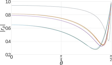
(a)

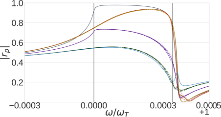
(b)

Figure 1: Absolute value of the reflection coefficient of a planar ZnSe surface. Left: reflection coefficient as function of incident angle $\theta$ at $\omega=\omega_{T}$. Right: reflection coefficient as function of frequency at $\theta=\pi/4$ with $\delta=0$ (solid lines), $\delta=0.5$ (doted) and $\delta=-0.5$ (dashed) and the color coding: Local (grey), HuyEx (red), Ting et al. (dark gold), Pekar (green), Agarwal et al. (indigo), Fuchs-Kliewer (brown), Rimbey-Mahan (ice blue).

It is evident that spatial dispersion significantly reduces the reflectivity for most of the angular spectrum at the transition frequency $\omega_{T}$. Only when the incident field arrives at a shallow angle, is the reflectivity increased. The Pekar and Rimbey-Mahan ABC’s predict the lowest reflectivity for frequencies smaller than $\omega_{L}$. The Fuchs-Kliewer and Ting et al. boundary conditions resemble the results obtained from the Huygens’ principle and the extinction theorem. In fact, the Fuchs-Kliewer boundary condition matches quite well the HuyEx results, although in a narrow frequency and angular interval, the transverse-longitudinal splitting $\delta\neq 0$ is less pronounced.

3 Thermal emissivity of an isolated spatially dispersive sphere

Now we turn to the thermal emissivity of a spatially dispersive sphere. The spectral energy flux mediated by the electromagnetic field from a sphere of radius $R$ at temperature $T_{sp}$ into free space through a surface $\mathcal{A}$ is given by

$$S(\omega,T_{sp})=\mu^{-1}_{0}\mathrm{Re}\int\limits_{\mathcal{A}}\mathrm{d}\mathbf{a}(\mathbf{r})\cdot\big{\langle}{\boldsymbol{E}}(\mathbf{r},\omega)\times{\boldsymbol{B}}^{\ast}(\mathbf{r},\omega)\big{\rangle}_{T_{sp}}$$ (28)

where $\langle...\rangle_{T_{sp}}$ denotes the thermal average over the spherical volume. The electromagnetic field $\mathbf{E}(\mathbf{r},\omega)$ is a solution of the Helmholtz equation. If we use the source quantity representation (4), we can write the expectation value as

$$\big{\langle}\mathbf{E}(\mathbf{r},\omega)\times\mathbf{B}^{\ast}(\mathbf{r}^{\prime},\omega)\big{\rangle}_{T}=-\mu^{3}_{0}\omega^{2}\int\limits_{V_{\mathrm{sp}}}\mathrm{d}^{3}s\int\limits_{V_{\mathrm{sp}}}\mathrm{d}^{3}s^{\prime}\mathrm{O_{c}}\big{\{}\boldsymbol{\mathcal{G}}(\mathbf{r},\mathbf{s})\cdot\big{\langle}\mathbf{j}(\mathbf{s},\omega)\otimes\mathbf{j}^{\ast}(\mathbf{s}^{\prime},\omega)\big{\rangle}_{T}\cdot\mathbf{\Gamma}^{\dagger}(\mathbf{r}^{\prime},\mathbf{s}^{\prime})\big{\}}\;,$$ (29)

where ${\boldsymbol{\Gamma}}(\mathbf{r},\mathbf{r^{\prime}},\omega)=-(i\mu_{0}\omega)^{-1}\nabla\times\boldsymbol{\mathcal{G}}(\mathbf{r},\mathbf{r}^{\prime},\omega)$ is again the magnetic dyadic Green function. We also introduced the outer vector product $\mathrm{O_{c}}\{\cdots\}$, which is defined as the curl between the outermost left and right vectors $\mathrm{O_{c}}\{\mathbf{A}\otimes\mathbf{B}\}=\mathbf{A}\times\mathbf{B}$. Note, that the vectors $\mathbf{r}$ and $\mathbf{r}^{\prime}$ remain outside $V_{\mathrm{sp}}$.

In thermal equilibrium and within linear response theory, we can apply the fluctuation-dissipation theorem to compute the thermal expectation value of the current density as

$$\big{\langle}\mathbf{j}(\mathbf{r},\omega)\otimes\mathbf{j}^{\ast}(\mathbf{r}^{\prime},\omega)\big{\rangle}_{T}=2\omega\epsilon_{0}\mathrm{Im}\boldsymbol{\mathcal{\epsilon}}(\mathbf{r},\mathbf{r}^{\prime},\omega)\Theta(\omega,T)\>.$$ (30)

Here, $\Theta(\omega,T)$ refers to the thermal distribution function $\Theta(\omega,T)=\hbar\omega/(e^{\hbar\omega/k_{b}T}-1)$. One can then derive the spectral heat transfer rate $S(\omega,T_{sp})$ in terms of the dyadic Greens function applying some algebra (for details, see App. B) as

$$S(\omega,T_{A})=\mu_{0}\omega\Theta(\omega,T)\mathrm{Im}\int\limits_{\mathcal{A}}\mathrm{d}\mathbf{a}(\mathbf{r})\cdot\int\limits_{\partial V_{\mathrm{sp}}}\mathrm{d}^{2}s\;\mathrm{O_{p}}\Big{\{}\big{[}\mathbf{n}(\mathbf{s})\times\boldsymbol{\mathcal{G}}^{T}(\mathbf{r},\mathbf{s})\big{]}\times\big{[}\mathbf{\Gamma}^{\ast}(\mathbf{r}^{\prime},\mathbf{s})\times\overleftarrow{\nabla}_{s}\big{]}$$

$$-\mathbf{n}(\mathbf{s})\times\big{[}\nabla_{s}\times\boldsymbol{\mathcal{G}}^{T}(\mathbf{r},\mathbf{s})\big{]}\times\mathbf{\Gamma}^{\ast}(\mathbf{r},\mathbf{s})\Big{\}}\;.$$ (31)

Here we introduced the notation for the outer scalar product $\mathrm{O_{p}}\{\cdots\}$ which is defined as the scalar product between the outermost left and right vectors $\mathrm{O_{p}}\{\mathbf{A}\otimes\mathbf{B}\}=\mathbf{A}\cdot\mathbf{B}$.

Equation (31) contains two surface integrals, one extends over the surface $\partial V_{sp}$ encapsulating the source region, the other covers the surface $\mathcal{A}$ through which the energy flux has to be computed. The latter is taken to be another spherical surface with radius $\rho>R$. We decompose the Green tensor into a freely propagating and a scattering part according to Eq. (6) which can be found in the literature, see e.g. Ref. [60]. In contrast to the local case, we use the reflection coefficients that take spatial dispersion into account. Performing the surface integrals and making use of the Wronskian of the spherical Hankel functions, we obtain a result that is independent of $\rho$,

$$S(\omega,T)=(k_{0}R)^{2}\Theta(\omega,T)e(\omega)$$ (32)

$$=-2k^{2}_{0}R^{2}\Theta(\omega,T)\sum\limits^{\infty}_{n=1}(2n+1)\big{(}\mathrm{Im}[\tilde{R}^{1,M}_{n}\tilde{R}^{2,M\ast}_{n}]+\mathrm{Im}[\tilde{R}^{1,N}_{n}\tilde{R}^{2,N\ast}_{n}]\big{)}.$$

where $e(\omega)$ denotes the spectral emissivity. This can be further simplified by applying the Wronskian once again to obtain

$$\mathrm{Im}[\tilde{R}^{1,X}_{n}\tilde{R}^{2,X\ast}_{n}]=\frac{\mathrm{Re}\big{[}r^{X}_{n}\big{]}}{k^{2}_{0}R^{2}}-\frac{|r^{X}_{n}|^{2}}{k^{2}_{0}R^{2}}$$ (34)

with $X\in\big{\{}\mathbf{M},\mathbf{N}\big{\}}$. This result corresponds to findings previously obtained in the local case [61].

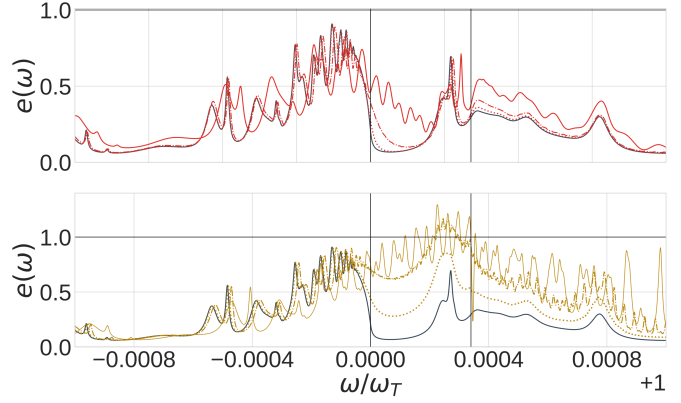
Figure 2: Depicts a comparison of local (black) versus the nonlocal spectral emissivity for a ZnSe sphere with $R=220$nm for different dispersion parameters: $D=D_{ZnSe}$ (solid), $D=D_{ZnSe}/10$ (dashed) and $D=D_{ZnSe}/100$ (dotted). The local case is compared to HuyEx (red, top) and Pekar (gold, bottom).

Figure 2 shows the emissivity of ZnSe as a function of frequency for a sphere of radius $R=220$nm resulting in a size parameter $k_{0}R=3.12>1$.

There is a noticeable difference between the local and nonlocal results. The overall emissivity is increased, and the spectral features are shifted towards higher frequencies. This is more pronounced for the Pekar ABC than for the HuyEx results. In both cases, the emissivity converges towards the local results with decreasing dispersion parameter $D=D_{ZnSe}$. The Pekar ABC predict plenty of spectral features, and the emissivity is highest within the stop band, exceeding $e(\omega)=1$. In contrast, the HuyEx results predict the maximum emissivity below the stop band and a lower emissivity.

We also notice that there are frequencies for which the emissivity is enhanced beyond the boundary of a perfect Planckian emitter, i.e. $e(\omega)>1$. That is a well-understood phenomenon [62, 63] which becomes more pronounced with decreasing radius. A perfect black body is one that absorbs all radiation incident on it. However, this standard definition has a geometric component to it. Due to the wave nature of light, this definition is only sensible when the size of the object is much larger than the wavelength. As soon as the size of an object becomes comparable to the wavelength, its geometric cross-section becomes smaller than the absorption/emission cross-section which implies that the emissivity can exceed $e(\omega)=1$.

4 Radiation driven near-field heat transfer between a sphere and a plate

We now turn to the problem of combining the emission from a sphere with that of a planar halfspace and compute the radiative heat transfer between them. We consider a plate $pl$ in the $(x,y)$ plane that occupies the entire lower half space $z\leq 0$. At a distance $d$ a sphere $sp$ with radius $R$ is embedded into free space. Its centre of mass is located at $z=d+R$, see Fig. 3. The sphere is held at a temperature $T_{sp}$ and the plate at temperature $T_{pl}$, respectively. We assume the temperatures to be constant, and the energy flow is mediated only by electromagnetic fields. Then both objects emit and absorb thermal radiation at a constant rate. It is sufficient to consider the effective energy transfer in one direction only, to establish the net heat transfer, we will apply the reciprocity condition.

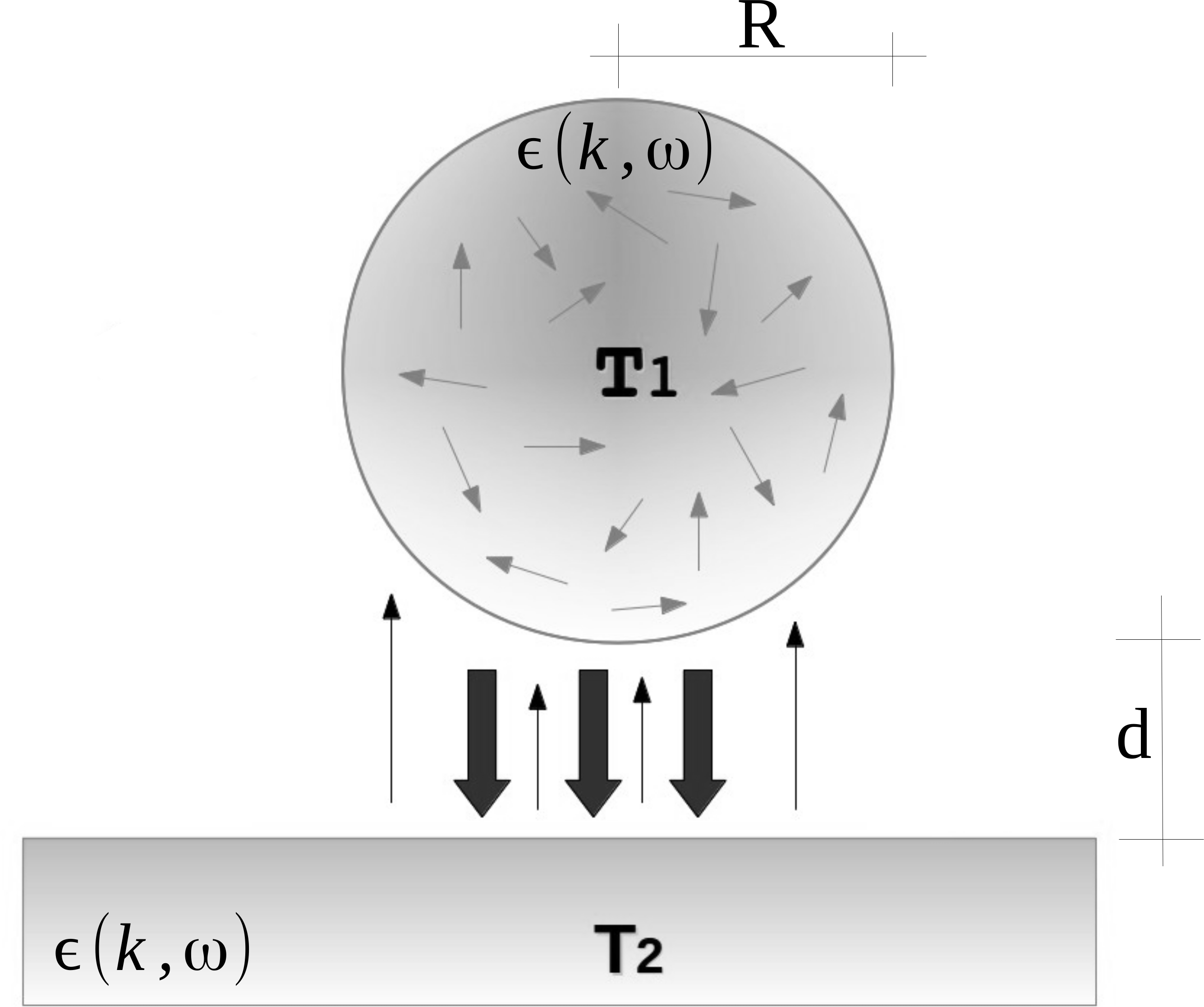
Figure 3: Schematic set up with a dielectric sphere of Radius $R$ at a distance $d$ above a dielectric half-space. Both are held at constant temperatures $T_{sp}$ and $T_{pl}$, respectively.

We begin this section by briefly reviewing the approach to heat transfer between dielectric bodies [64] and introduce the necessary modifications to include spatial dispersion. In the previous sections, we have presented the derivation of the plate reflection coefficients and the emissivity of an isolated sphere. In each derivation, we required basis vectors of their particular geometry, i.e. either vector spherical or cylindrical harmonics. For the joint geometry of plate and sphere, it will be necessary to interconvert between the bases.

Let ${\boldsymbol{\Psi}}^{(\pm)}_{\alpha}(k,\mathbf{r})$ represent the set of vector spherical harmonics, where $\alpha=\{\mathbf{P},n,m\}$ is a multi-index containing the polarisation $\mathbf{P}\in\{\mathbf{M},\mathbf{N}\}$ and the indices $n\in\mathbb{N}$ as well as $m\in\big{[}-n,n\big{]}$. The origin of the vector spherical harmonics is at the centre of the sphere. The superscript $(\pm)$ denotes an outgoing $(+)$ or an incoming wave $(-)$, relative to the origin of the reference frame, and requires one to replace the Bessel function by the Hankel function of the first kind (superscript $(+)\rightarrow(1)$) and the Hankel function of the second kind (superscript $(-)\rightarrow(2)$), respectively. In this notation the electric field outside an isolated, radiating sphere becomes

$$\mathbf{E}_{sp}(\mathbf{r},\omega)=\sum\limits_{\alpha}\mathcal{A}^{0}_{\alpha+}{\boldsymbol{\Psi}}^{(+)}_{\alpha}(k_{0},\mathbf{r}).$$ (35)

It describes waves propagating away from the sphere with amplitude $\mathcal{A}^{0}_{\alpha+}$. In this notation, Eqs. (28) and (LABEL:SpEmission) become

$$\big{\langle}\mathbf{E}_{sp}(\mathbf{r},\omega)\times\mathbf{B}_{sp}^{*}(\mathbf{r}^{\prime},\omega)\big{\rangle}_{T}=\mathcal{N}(\omega,T)e_{\alpha}(\omega){\boldsymbol{\Psi}}^{(+)}_{\alpha}(k_{0},\mathbf{r})\times\big{[}\nabla^{\prime}\times{\boldsymbol{\Psi}}^{(+)*}_{\alpha,}(k_{0},\mathbf{r}^{\prime})\big{]}$$

$$=-i\omega\big{\langle}\mathcal{A}^{0}_{\alpha_{+}}\mathcal{A}^{0*}_{\alpha_{+}}\big{\rangle}_{T}{\boldsymbol{\Psi}}^{(+)}_{\alpha}(k_{0},\mathbf{r})\times\big{[}\nabla^{\prime}\times{\boldsymbol{\Psi}}^{(+)*}_{\alpha}(k_{0},\mathbf{r}^{\prime})\big{]},$$ (36)

where we introduced the variables

$$e_{\alpha}(\omega)=2ik_{0}\mathrm{Im}[\tilde{R}^{1,P}_{n}\tilde{R}^{2,P*}_{n}]\big{(}\delta_{\mathbf{P},\mathbf{N}}+\delta_{\mathbf{P},\mathbf{M}}\big{)},$$

$$\mathcal{N}(\omega,T)=\mu_{0}k^{2}_{0}R^{2}\Theta(\omega,T).$$ (37)

For the plate reference system we already introduced the vector cylindrical harmonics, here denoted by ${\boldsymbol{\phi}}^{(\pm)}_{\beta}(\mathbf{k},\mathbf{r})$. The multi-index $\beta\in\{\mathbf{P},n\}$ contains the polarisation $\mathbf{M},\mathbf{N}$ and $n\in\mathbb{N}$. The point of origin is on the plate surface closest to the sphere, i.e. the direction of the $z$-axis points to the centre of the sphere. The superscript $\pm$ refers to outgoing or incoming waves, relative to the origin of the plate reference frame.

While Eqs. (35) and (36) describe the field emitted by an isolated sphere, we require the knowledge of the total emitted field including multiple reflections between the sphere and the plate. The total electromagnetic field emitted, by the sphere, and in cylindrical coordinates with the origin at the plate interface, shall hereby be denoted with

$$\mathbf{E}^{tot}_{sp}(\mathbf{r},\omega)=\sum\limits_{\beta}\mathcal{B}_{\beta}{\boldsymbol{\phi}}^{(+)}_{\beta}(\mathbf{k}_{0},\mathbf{r}).$$ (38)

The thermal expectation value of the vector product of the electric and magnetic field becomes

$$\big{\langle}\mathbf{E}(\mathbf{r},\omega)\times\mathbf{B}^{*}(\mathbf{r}^{\prime},\omega)\big{\rangle}_{T}=-i\omega\sum\limits_{\beta^{\prime},\beta}\big{\langle}\mathcal{B}_{\beta}\mathcal{B}_{\beta^{\prime}}\big{\rangle}_{T}{\boldsymbol{\phi}}^{(+)}_{\beta}(\mathbf{k}_{0},\mathbf{r})\times\big{[}\nabla\times{\boldsymbol{\phi}}^{(+)*}_{\beta^{\prime}}(\mathbf{k}_{0},\mathbf{r}^{\prime})\big{]}\;.$$ (39)

Next, we relate the amplitudes $\mathcal{A}^{0}_{\alpha_{+}}$ of a wave emitted by an isolated sphere to its total amplitude $\mathcal{B}_{\beta}$ in the presence of a plate. The conversion is described by an operator $\mathbb{O}_{\beta\alpha_{+}}$ as

$$\mathcal{B}_{\beta}=\sum\limits_{\alpha}\mathbb{O}_{\beta\alpha_{+}}\mathcal{A}^{0}_{\alpha_{+}}.$$ (40)

To determine this operator we consider a mode $\Pi\in\{\mathbf{M}_{nm},\mathbf{N}_{nm}\}$ of spherical waves, emanating from the sphere ${\boldsymbol{\Psi}}^{(+)}_{\alpha}$ and a corresponding mode emanating from the plate ${\boldsymbol{\phi}}^{(\pm)}_{\beta}$. The resulting electric field $\mathbf{E}^{\Pi}$ in the vacuum region is then given as a superposition

$$\mathbf{E}^{\Pi}(\mathbf{r},\omega)=\sum\limits_{\alpha}\mathcal{A}^{\Pi}_{\alpha_{+}}{\boldsymbol{\Psi}}^{(+)}_{\alpha}(k_{0},\mathbf{r})+\sum\limits_{\beta}\mathcal{B}^{\Pi}_{\beta_{+}}{\boldsymbol{\phi}}^{(+)}_{\beta}(\mathbf{k}_{0},\mathbf{r}).$$ (41)

It is useful to introduce another operator $\Lambda_{yx}$ that transforms vector spherical into cylindrical waves or vice versa [65]. An incoming spherical wave is partially reflected at the plate, which is the only source of cylindrical waves. Hence, we can write

$$\mathcal{B}^{\Pi}_{\beta_{+}}=R_{\beta+\beta^{\prime}-}\Lambda_{\beta_{-}^{\prime},\alpha_{+}}\mathcal{A}^{\Pi}_{\alpha_{+}},$$ (42)

where $R_{\beta+\beta^{\prime}-}$ are the reflection coefficients in cylindrical coordinates of the plate, which we derived in Sec. 2. An outgoing spherical wave with amplitude $\mathcal{A}^{\Pi}_{\alpha_{+}}$ can be generated by an emission $\mathcal{A}^{0}_{\alpha_{+}}$ or by reflection of an impinging cylindrical wave at the surface of the sphere. Thus we find

$$\mathcal{A}^{\Pi}_{\alpha_{+}}=\mathcal{A}^{0}_{\alpha_{+}}\delta_{\alpha_{+}\Pi}+r_{\alpha_{+}\alpha_{-}^{\prime}}\Lambda_{\alpha_{-}^{\prime},\beta_{+}}\mathcal{B}^{\Pi}_{\beta_{+}}.$$ (43)

Combined with Eq. (42) we obtain a conditional equation for the total amplitude $A^{\Pi}_{\alpha_{+}^{\prime}}$

$$\Big{[}\delta_{\alpha_{+},\alpha_{+}^{\prime}}-T_{\alpha_{+},\alpha_{+}^{\prime}}\Big{]}\mathcal{A}^{\Pi}_{\alpha_{+}^{\prime}}=\mathcal{A}^{0}_{\alpha_{+}^{\prime}}\delta_{\alpha_{+}^{\prime}\Pi}\;,$$ (44)

with

$$T_{\alpha_{+},\alpha_{+}^{\prime}}=r_{\alpha_{+}\tilde{\alpha}_{-}}\Lambda_{\tilde{\alpha}_{-},\beta_{+}^{\prime}}R_{\beta^{\prime}_{+}\beta_{-}}\Lambda_{\beta_{-},\alpha_{+}^{\prime}}.$$ (45)

Once the amplitudes $\mathcal{A}^{\Pi}_{\alpha_{+}}$ are determined from Eq. (44), one is able to derive an expression for the conversion operator

$$\mathbb{O}_{\beta\alpha+}=\tau_{\beta_{+}\beta_{-}^{\prime}}\Lambda_{\beta_{-}^{\prime},\alpha_{+}^{\prime}}\Big{[}\delta_{\alpha_{-},\alpha_{+}^{\prime}}-T_{\alpha_{+},\alpha_{+}^{\prime}}\Big{]}^{-1}\;.$$ (46)

We are only interested in the radiation absorbed by the half space, which is represented by the transmission coefficients $\tau_{\beta\beta^{\prime}}$. However, $\tau_{\beta\beta^{\prime}}$ is a diagonal matrix, and only the absolute square will contribute. Hence, we can replace $|\tau_{\beta\beta^{\prime}}|^{2}$ with $1-|R_{\beta,\beta^{\prime}}|^{2}$. Together with Eq. (44), we can write the Poynting vector as a function of the total emission coefficients

$$S(\omega,T)=\mu^{-1}_{0}\mathrm{Re}\int\limits_{\mathcal{A}}\mathrm{d}\mathbf{a}(\mathbf{r})\cdot\big{\langle}\mathbf{E}(\mathbf{r},\omega)\times\mathbf{B}^{*}(\mathbf{r},\omega)\big{\rangle}_{T}$$

$$=\mathbb{S}_{\alpha_{+},\alpha_{+}^{\prime}}\big{\langle}\mathcal{A}^{\Pi}_{\alpha_{+}}\mathcal{A}^{\Pi*}_{\alpha_{+}^{\prime}}\big{\rangle}_{T}\;.$$ (47)

They in return depend on the emission coefficients of an isolated sphere as in Eq. (36) through

$$\mathbb{S}_{\alpha_{+},\alpha_{+}^{\prime}}=\Lambda^{\dagger}_{\beta_{-}^{\prime},\alpha_{+}}\tau^{\dagger}_{\beta_{+}\beta_{-}^{\prime}}\mathbb{I}_{\beta_{-}\tilde{\beta}_{+}}\tau_{\tilde{\beta}_{+}\tilde{\beta}_{-}^{\prime}}\Lambda_{\tilde{\beta}_{-}^{\prime},\alpha_{+}^{\prime}}$$ (48)

with the corresponding surface integral

$$\mathbb{I}_{\beta\beta^{\prime}}=\mu^{-1}_{0}\mathrm{Re}\int\limits_{\partial V_{pl}}\mathrm{d}\mathbf{a}(\mathbf{r})\cdot{\boldsymbol{\phi}}_{\beta}(\mathbf{k}_{0},\mathbf{r})\times\big{[}\nabla\times{\boldsymbol{\phi}}^{*}_{\beta^{\prime}}(\mathbf{k}_{0},\mathbf{r})\big{]}.$$ (49)

This integral can be solved analytically and only the diagonal terms with $\beta=\beta^{\prime}$ do not vanish. In the nonlocal case, this simplifies the computation significantly as we can use the results from Sec. 2.

The heat transfer in the nonequilibrium case where the half-space is at temperature $T_{pl}$ and the sphere at $T_{sp}$ is obtained by applying the reciprocity argument [66]. The net heat transfer can then be written as

$$Q(T_{pl},T_{sp})=Q(T_{pl},0)+Q(0,T_{sp})$$

$$=\int\frac{\mathrm{d}\omega}{2\pi}\;\big{[}S(\omega,T_{pl})-S(\omega,T_{sp})\big{]},$$

$$=\int\frac{\mathrm{d}\omega}{2\pi}\;\big{[}\Theta(\omega,T_{pl})-\Theta(\omega,T_{sp})\big{]}\mathcal{T}(\omega).$$ (50)

where the last equation has been cast into the Landauer-like form [67, 63] by introducing the transmissivity $\mathcal{T}(\omega)$ which will be of use in the next section.

4.1 Numerical Results

We now apply our results to numerically compute the heat transfer rate between a ZnSe sphere and half-space using the dielectric function for ZnSe given by Eq. (9). The temperature of the sphere is $k_{B}T_{sp}=\hbar\omega_{T}$ and that of the plate is taken to be 5$\%$ smaller.

In order to compute $\mathcal{T}(\omega)$ and $S(T)$ we have to solve Eq. (44) for the spherical scattering amplitudes $\mathcal{A}^{\Pi}_{\alpha_{+}^{\prime}}$. To this end, we introduce a cutoff at $n=n_{max}$ which we chose such that $n_{max}=8+2.5k_{0}R+R/d$. Finally, we use these result in Eq. (47) to obtain the heat flux spectral density $S(\omega,T)$, from which we obtain $S(T)$ by integrating over the frequency with an adaptive Gauss quadrature method. For more details on the numerical convergence and scaling properties of this method, we refere the reader to Ref. [64].

In Fig. 4 we show the transmissivity $\mathcal{T}(\omega)$ for a sphere of Radius $R=220$ nm as function of frequency. In the upper panel, the far-field spectrum is shown for $d=3600nm$, roughly eight times the transition wavelength. In the lower panel, the gap distance is only $d=1$nm.

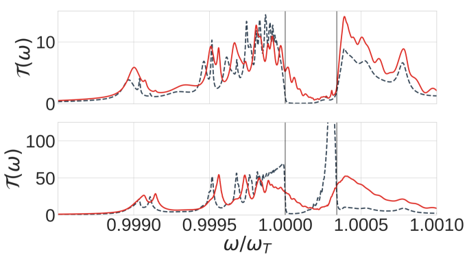
Figure 4: Spectral transmissivity for a ZnSe sphere with radius $R=220$nm and gap distance to a ZnSe plate of $d=3600$nm (top) and $d=1$nm (bottom) with the colour coding: local (dashed, grey) and HuyEx (solid, red).

In the far-field spectrum, one observes the expected suppressed transmissivity within the stopband $\omega_{T}<\omega<\omega_{L}$. In the nonlocal case, this effect is enhanced. The previously observed frequency shifts in the emissivity are retained. It is apparent that the overall transmissivity in the nonlocal case is enhanced. From this, it follows that heat transfer rate is increased as well. In the lower panel of Fig. 4 the gap distance is much smaller than the transition wavelength $d\ll\lambda_{T}$. Hence, evanescent modes govern the heat transfer rate. Below the transverse resonance frequency $\omega_{T}$, one observes the influence of the whispering gallery modes, and within the stop band, the enhancement of the surface guided modes dominate the spectrum. In the local case and for $n_{max}=60$ these modes peak at $\mathcal{T}\approx 400$, beyond the shown region.

When comparing the far-field spectrum with the near-field spectrum, one observes the enhancement in the transmissivity due to surface guided modes. We expect nonlocal contributions to dominate the resonances whenever the gap distance is in the order of $d\sim\sqrt{D4\pi^{2}/\omega^{2}_{T}}\approx 1.2$nm. This is indeed evident from Fig. 4. The surface resonance is suppressed, broadened and shifted towards higher frequencies.

In Fig. 5 the heat transfer rate $S(d)/S_{0}$ is shown as a function of distance, where the normalisation $S_{0}$ is simply the value of $S(d)$ at $d=3600$nm (far-field). It is worth noting that $S_{0}$ in the nonlocal case is $36.5\%$ larger than its local analogue. This is evident from the top panel in Fig. 4 as the nonlocal spectrum, beyond the transition frequency $\omega_{T}$, exceeds the local spectrum. At short distances $d\lesssim 100$nm, both curves diverge from one another, with the result for the spatially dispersive material levelling out at a constant value. Hence, the inclusion of spatial dispersion removes the divergent behaviour due to the damping of the surface guided modes (Fig. 4). The removal of the spurious divergence that occurs in a local theory is consistent with recent studies of heat transfer between planar boundaries [59, 19]. However, the absolute length scales at which the heat transfer rate tails off is already so small that any macroscopic approach could be questionable, and other effects might become important.

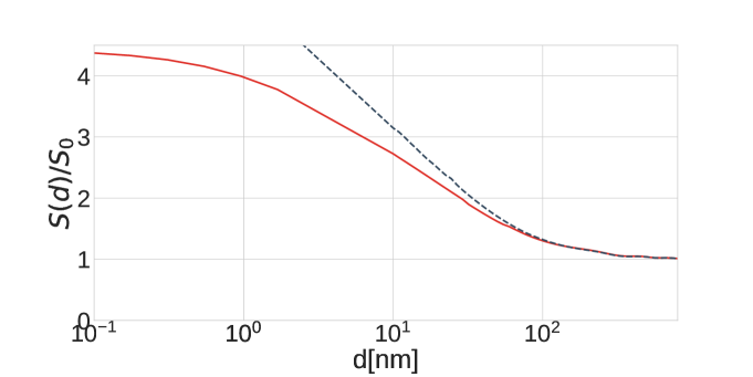
Figure 5: Heat transfer rate as a function of distance. The nonlocal HuyEx (solid, red) results level off at short distances, while the local (dashed, grey) case shows the typical spurious divergence at short distances.

5 Summary

We have utilised Huygens’ principle and the extinction theorem (HuyEx) to derive the reflection coefficients for a spatially dispersive half-space. We found the reflection coefficients to be dependent on surface impedances, which can be evaluated for arbitrary homogeneous and isotropic spatially dispersive dielectric functions. Numerical results for ZnSe material have shown a remarkable resemblance to results obtained with the Fuchs and Kliever ABC’s for most of the frequency and angular spectrum, apart from the longitudinal and transverse splitting which, in the vicinity of the longitudinal resonance frequency $\omega_{L}$, is more pronounced for Maxwell boundary conditions.

Based on the fluctuation dissipation theorem, we derived the emissivity of an isolated spatially dispersive sphere. We compared the HuyEx and Pekar ABC’s to the local results and found significant differences for a ZnSe sphere of radius $R=220$ nm. The overall emissivity is enhanced in both nonlocal cases. The ABC’s spectrum shows an increased number of resonances, and in contrast to the HuyEx and local case, the maximal emissivity lies within the stop band. The HuyEx emissivity is much more similar to the local result. The peaks are shifted towards higher frequencies, and additional resonances appear above $\omega_{T}$.

Finally, we used an exact mode matching method to investigate the influence of spatial dispersion on the near-field heat transfer. We found a significant impact of spatial dispersion on the spectral heat transfer rate. In particular, the surface guided modes are suppressed, blue shifted and broadened compared to the local analogue. As a consequence and in contrast to the local case, the heat transfer rate levels off at small distances, thereby removing the spurious divergences that plague local theories.

Appendix A Basis vectors and orthogonality relations

A.1 Vector cylindrical harmonics

The vector wave function in cylindrical coordinates used in this article are defined as

$$\mathbf{M}_{n}(\mathbf{k},\mathbf{r})=\frac{\mathcal{N}_{n}}{q}\nabla\times\mathbf{e}_{z}J_{n}(q\rho)e^{i\beta z+in\phi},$$

$$\mathbf{N}_{n}(\mathbf{k},\mathbf{r})=\frac{\mathcal{N}_{n}}{qk}\nabla\times\nabla\times\mathbf{e}_{z}J_{n}(q\rho)e^{i\beta z+in\phi},$$

$$\mathbf{L}_{n}(\mathbf{k},\mathbf{r})=\frac{1}{k}\mathcal{N}_{n}\nabla J_{n}(q\rho)e^{i\beta z+in\phi}$$ (51)

with the normalisation constant $\mathcal{N}_{n}=i^{n}/2\pi$. Note that $(-1)^{n}\mathcal{N}_{-n}=\mathcal{N}_{n}$. The normalisation constants are chosen such that the vector cylindrical harmonics are orthonormal, i.e.

$$\int\mathrm{d}^{3}r\mathbf{M}_{n}(\mathbf{k},\mathbf{r})\cdot\mathbf{M}_{-n^{\prime}}(-\mathbf{k}^{\prime},\mathbf{r})=\delta_{n,n^{\prime}}\delta(\beta-\beta^{\prime})\frac{\delta(\mathbf{q}-\mathbf{q}^{\prime})}{q},$$

$$\int\mathrm{d}^{3}r\mathbf{N}_{n}(\mathbf{k},\mathbf{r})\cdot\mathbf{N}_{-n^{\prime}}(-\mathbf{k}^{\prime},\mathbf{r})=\delta_{n,n^{\prime}}\delta(\beta-\beta^{\prime})\frac{\delta(\mathbf{q}-\mathbf{q}^{\prime})}{q},$$

$$\int\mathrm{d}^{3}r\mathbf{L}_{n}(\mathbf{k},\mathbf{r})\cdot\mathbf{L}_{-n^{\prime}}(-\mathbf{k}^{\prime},\mathbf{r})=\delta_{n,n^{\prime}}\delta(\beta-\beta^{\prime})\frac{\delta(\mathbf{q}-\mathbf{q}^{\prime})}{q}.$$ (52)

A.2 Field expansion

We require an expansion of the field into components orthogonal to the surface and parallel to it. For this purpose we introduce a new orthonormal basis

$$\mathbf{X}_{n}(\mathbf{q},\phi,\rho)=\tilde{\mathcal{N}}_{n}J_{n}(q\rho)e^{in\phi}\mathbf{e}_{q},$$

$$\mathbf{e}_{z}\times\mathbf{X}_{n}(\mathbf{q},\phi,\rho)=-\tilde{\mathcal{N}}_{n}J_{n}(q\rho)e^{in\phi}\mathbf{e}_{q}\times\mathbf{e}_{z},$$

$${\boldsymbol{\chi}}_{n}(\mathbf{q},\phi,\rho)=\tilde{\mathcal{N}}_{n}J_{n}(q\rho)e^{in\phi}\mathbf{e}_{z},$$ (53)

with $\tilde{\mathcal{N}}_{n}=\frac{i^{n}}{\sqrt{2\pi}}$. They obey the orthogonality relations

$$\int\mathrm{d}\phi\int\mathrm{d}\rho\rho\mathbf{X}_{n}(\mathbf{q},\phi,\rho)\cdot\mathbf{X}_{-n^{\prime}}(-\mathbf{q}^{\prime},\phi,\rho)=-\frac{\delta(q-q^{\prime})}{q}\delta_{nn^{\prime}},$$

$$\int\mathrm{d}\phi\int\mathrm{d}\rho\rho\big{[}\mathbf{e}_{z}\times\mathbf{X}_{n}(\mathbf{q},\phi,\rho)\big{]}\cdot\big{[}\mathbf{e}_{z}\times\mathbf{X}_{-n^{\prime}}(-\mathbf{q}^{\prime},\phi,\rho)\big{]}=-\frac{\delta(q-q^{\prime})}{q}\delta_{nn^{\prime}},$$

$$\int\mathrm{d}\phi\int\mathrm{d}\rho\rho{\boldsymbol{\chi}}_{n}(\mathbf{q},\phi,\rho)\cdot{\boldsymbol{\chi}}_{-n^{\prime}}(-\mathbf{q}^{\prime},\phi,\rho)=\frac{\delta(q-q^{\prime})}{q}\delta_{nn^{\prime}}.$$ (54)

They are connected to the vector cylindrical harmonics as

$$\mathbf{M}_{n}(\mathbf{k},\mathbf{r})=-i\frac{1}{\sqrt{2\pi}}e^{i\beta z}\mathbf{e}_{z}\times\mathbf{X}_{n}(\mathbf{q},\phi,\rho),$$

$$\mathbf{N}_{n}(\mathbf{k},\mathbf{r})=\frac{1}{\sqrt{2\pi}}\frac{1}{k}e^{i\beta z}\big{[}q{\boldsymbol{\chi}}_{n}(\mathbf{q},\phi,\rho)-\beta\mathbf{X}_{n}(\mathbf{q},\phi,\rho)\big{]},$$

$$\mathbf{L}_{n}(\mathbf{k},\mathbf{r})=\frac{1}{\sqrt{2\pi}}\frac{i}{k}e^{i\beta z}\big{[}\beta{\boldsymbol{\chi}}_{n}(\mathbf{q},\phi,\rho)+q\mathbf{X}_{n}(\mathbf{q},\phi,\rho)\big{]}.$$ (55)

A.3 Important relations and basis transformations

In equation 25 we derived the reflection coefficients $R_{s}$ and $R_{q}$ in the basis of Eq. (A.2). we are interested in the relation between these reflection coefficients and the corresponding reflection coefficients in the basis of vector cylindrical harmonics $r_{s}$, $r_{p}$. Let the field $\mathbf{F}(\mathbf{r})$ be in the basis of Eq. (16). Then,

$$\alpha_{n}(\mathbf{q},\beta)=\int\mathrm{d}^{2}r\mathbf{F}(\mathbf{r})\cdot\mathbf{M}_{-n}(-\mathbf{q},-\beta,\mathbf{r})$$

$$=\sum_{n^{\prime}}\int\mathrm{d}z\int\mathrm{d}q\;qA_{n^{\prime}}(\mathbf{q},z)i\frac{e^{-i\beta z}}{\sqrt{2\pi}}\frac{\delta(q-q^{\prime})}{q}\delta_{nn^{\prime}}.$$ (56)

For the incoming field we may choose

$$\alpha^{inc}_{n}(\mathbf{q},\beta)=\alpha^{inc}_{n}(\mathbf{q}_{0},\beta_{0})\frac{\delta(q-q_{0})}{q}\delta(\beta+\beta_{0})$$

$$=\int\mathrm{d}zA^{inc}_{n}(\mathbf{q},z)i\frac{e^{-i\beta z}}{\sqrt{2\pi}}.$$ (57)

The term $\delta(\beta+\beta_{0})$ takes the direction of the incoming wave, traveling into the $-z$ direction, into account. We can also derive $A^{inc}_{n}(\mathbf{q},z)$ in terms of $\alpha^{inc}_{n}(\mathbf{q},\beta)$ and find

$$A^{inc}_{n}(\mathbf{q},z)=-\int\mathrm{d}^{3}r\mathbf{F}(\mathbf{r})\cdot\mathbf{e}_{z}\times\mathbf{X}_{-n}(-\mathbf{q},-\beta,\mathbf{\rho})$$

$$=-\frac{i}{\sqrt{2\pi}}\int\mathrm{d}\beta e^{i\beta z}\alpha_{n}(\mathbf{q},\beta),$$

$$A^{inc}_{n}(\mathbf{q},z)=-\frac{i}{\sqrt{2\pi}}\alpha^{inc}_{n}(\mathbf{q}_{0},\beta_{0})\frac{\delta(q-q_{0})}{q}\frac{e^{-i\beta_{0}z}}{\sqrt{2\pi}}.$$ (58)

In order to expand the reflection amplitudes in terms of reflection coefficients,

$$A^{scat}_{n}(\mathbf{q},z)=A^{inc}_{n}(\mathbf{q},0)R_{s}(\mathbf{q},z),$$

we decompose $\alpha^{scat}_{n}(\mathbf{q},\beta)$ by writing $\alpha^{scat}_{n}(\mathbf{q},\beta)=r_{s}(\mathbf{q},\beta)\alpha^{inc}_{n}(\mathbf{q},-\beta)$, taking into account that the scattered field travels in the opposite $z$ direction to the incoming field. Thus, we find

$$A^{scat}_{n}(\mathbf{q},z)=A^{inc}_{n}(\mathbf{q},0)R_{s}(\mathbf{q},z)=\frac{i}{\sqrt{2\pi}}\int\mathrm{d}\beta e^{i\beta z}\alpha_{n}(\mathbf{q},\beta)$$

$$=\frac{i}{\sqrt{2\pi}}r_{s}(\mathbf{q},\beta_{0})\alpha^{inc}_{n}(\mathbf{q}_{0},\beta_{0})\frac{\delta(q-q_{0})}{q}\frac{e^{i\beta_{0}z}}{\sqrt{2\pi}}.$$ (59)

Using the above and $R_{s}(\mathbf{q},z)=R_{s}(\mathbf{q})e^{i\beta z}$ we obtain

$$R_{s}(\mathbf{q}_{0})=r_{s}(\mathbf{q}_{0},\beta_{0}).$$ (60)

Similarly, we can relate $R_{q}$ with $r_{p}$. Therefore we need to take into account that the incoming and reflected field are transversal only. Hence $\gamma_{n}$ in Eq. (14) vanishes. As a consequence $B^{(0)}_{n}$ and $C^{(0)}_{n}$ are linear dependent. In analogy to the above procedure, we find

$$r_{p}(\mathbf{q}_{0},\beta_{0})=-R_{q}(\mathbf{q}_{0}).$$ (61)

Appendix B Algebraic transformation of the fluctuation-dissipation theorem

In this appendix we derive Eq. (31). The starting point is Eq. (29) together with the fluctuation-dissipation theorem Eq. (30),

$$\big{\langle}\mathbf{E}(\mathbf{r},\omega)\times\mathbf{B}^{*}(\mathbf{r}^{\prime},\omega)\big{\rangle}_{T}=-2\epsilon_{0}\mu^{3}_{0}\omega^{3}\Theta(\omega,T)\int\limits_{V_{\mathrm{sp}}}\mathrm{d}^{3}s\int\limits_{V_{\mathrm{sp}}}\mathrm{d}^{3}s^{\prime}\mathrm{O_{c}}\big{\{}\boldsymbol{\mathcal{G}}(\mathbf{r},\mathbf{s})\cdot\mathrm{Im}\boldsymbol{\mathcal{\epsilon}}(\mathbf{s},\mathbf{s}^{\prime},\omega)\cdot\mathbf{\Gamma}^{\dagger}(\mathbf{r}^{\prime},\mathbf{s}^{\prime})\big{\}}.$$ (62)

If we split the imaginary part of the dielectric tensor into $\mathrm{Im}\boldsymbol{\mathcal{\epsilon}}(\mathbf{s},\mathbf{s}^{\prime})=(2i)^{-1}\big{[}\boldsymbol{\mathcal{\epsilon}}(\mathbf{s},\mathbf{s}^{\prime})-\boldsymbol{\mathcal{\epsilon}}^{*}(\mathbf{s},\mathbf{s}^{\prime})\big{]}$, and use the Helmholtz equation for the Green tensor, we can eliminate the dielectric tensor from Eq. (62) and find

$$\big{\langle}\mathbf{E}(\mathbf{r},\omega)\times\mathbf{B}^{*}(\mathbf{r}^{\prime},\omega)\big{\rangle}_{T}=i\mu^{2}_{0}\omega\Theta(\omega,T)\mathrm{O_{c}}\bigg{\{}$$

$$\int\limits_{V_{\mathrm{sp}}}\mathrm{d}^{3}s^{\prime}\big{[}\boldsymbol{\mathcal{G}}(\mathbf{r},\mathbf{s}^{\prime})\times\overleftarrow{\nabla}_{s^{\prime}}\times\overleftarrow{\nabla}_{s^{\prime}}-\boldsymbol{\mathcal{I}}\delta(\mathbf{r}-\mathbf{s}^{\prime})\big{]}\cdot\mathbf{\Gamma}^{\dagger}(\mathbf{r}^{\prime},\mathbf{s}^{\prime})$$

$$-\int\limits_{V_{\mathrm{sp}}}\mathrm{d}^{3}s\,\boldsymbol{\mathcal{G}}(\mathbf{r},\mathbf{s})\cdot\big{[}\nabla_{s}\times\nabla_{s}\times\mathbf{\Gamma}^{\dagger}(\mathbf{r}^{\prime},\mathbf{s})-\frac{\boldsymbol{\mathcal{I}}\delta(\mathbf{s}-\mathbf{r}^{\prime})}{i\mu_{0}\omega}\times\overleftarrow{\nabla}_{r^{\prime}}\big{]}\bigg{\}}.$$ (63)

Note that both integrals over $s$ and $s^{\prime}$ are finite volume integrals and the points $\mathbf{r}$ and $\mathbf{r}^{\prime}$ are located outside this volume. Thus, the delta function terms do not contribute to the integrals. Hence, we can write

$$\big{\langle}\mathbf{E}(\mathbf{r},\omega)\times\mathbf{B}^{*}(\mathbf{r}^{\prime},\omega)\big{\rangle}_{T}=i\mu^{2}_{0}\omega\Theta(\omega,T)\mathrm{O_{c}}\bigg{\{}\int\limits_{V_{\mathrm{sp}}}\mathrm{d}^{3}s\bigg{[}\boldsymbol{\mathcal{G}}(\mathbf{r},\mathbf{s})\times\overleftarrow{\nabla}_{s}\times\overleftarrow{\nabla}_{s}\cdot\mathbf{\Gamma}^{\dagger}(\mathbf{r^{\prime}},\mathbf{s})$$

$$-\boldsymbol{\mathcal{G}}(\mathbf{r},\mathbf{s})\cdot\big{[}\nabla_{s}\times\nabla_{s}\times\mathbf{\Gamma}^{\dagger}(\mathbf{r}^{\prime},\mathbf{s})\big{]}\bigg{]}\bigg{\}}\;.$$ (64)

It is convenient to eliminate the outer curl and transform the volume integral into a surface integral by applying the vector Green theorem. For this reason we first transform the outer vector product into an outer product

$$\mathrm{O_{c}}\big{\{}\big{(}\big{(}\boldsymbol{\mathcal{G}}(\mathbf{r},\mathbf{s})\times\overleftarrow{\nabla}_{s}\big{)}\times\overleftarrow{\nabla}_{s}\big{)}\cdot\mathbf{\Gamma}^{\dagger}(\mathbf{r^{\prime}},\mathbf{s})\big{\}}=\mathrm{O_{p}}\big{\{}\nabla_{s}\times\nabla_{s}\times\boldsymbol{\mathcal{G}}^{T}(\mathbf{r},\mathbf{s})\times\mathbf{\Gamma}^{*}(\mathbf{r}^{\prime},\mathbf{s})\big{\}},$$

$$\mathrm{O_{c}}\big{\{}\boldsymbol{\mathcal{G}}(\mathbf{r},\mathbf{s})\cdot\big{(}\nabla_{s}\times\big{(}\nabla_{s}\times\mathbf{\Gamma}^{\dagger}(\mathbf{r}^{\prime},\mathbf{s})\big{)}\big{)}\big{\}}=\mathrm{O_{p}}\big{\{}\boldsymbol{\mathcal{G}}^{T}(\mathbf{r},\mathbf{s})\times\big{(}\mathbf{\Gamma}^{*}(\mathbf{r}^{\prime},\mathbf{s})\times\overleftarrow{\nabla}_{s}\big{)}\times\overleftarrow{\nabla}_{s}\big{\}}\;.$$ (65)

This can be applied to

$$\nabla_{s}\cdot\mathrm{O_{c}}\big{\{}\big{[}\nabla_{s}\times\boldsymbol{\mathcal{G}}^{T}(\mathbf{r},\mathbf{s})\big{]}\times\mathbf{\Gamma}^{*}(\mathbf{r}^{\prime},\mathbf{s})\big{\}}=\mathrm{O_{p}}\big{\{}\nabla_{s}\times\big{(}\nabla_{s}\times\boldsymbol{\mathcal{G}}^{T}(\mathbf{r},{\bf s})\big{)}\times\mathbf{\Gamma}^{*}(\mathbf{r}^{\prime},\mathbf{s})\big{\}}$$

$$+\mathrm{O_{p}}\big{\{}\nabla_{s}\times\boldsymbol{\mathcal{G}}^{T}(\mathbf{r},\mathbf{s})\times\big{(}\mathbf{\Gamma}^{*}(\mathbf{r}^{\prime},\mathbf{s})\times\overleftarrow{\nabla}_{s}\big{)}\big{\}},$$

$$\nabla_{s}\cdot\mathrm{O_{c}}\big{\{}\boldsymbol{\mathcal{G}}^{T}(\mathbf{r},\mathbf{s})\times\big{[}\mathbf{\Gamma}^{*}(\mathbf{r}^{\prime},\mathbf{s})\times\overleftarrow{\nabla}_{s}\big{]}\big{\}}=\mathrm{O_{p}}\big{\{}\nabla_{s}\times\boldsymbol{\mathcal{G}}^{T}(\mathbf{r},\mathbf{s})\times\mathbf{\Gamma}^{*}(\mathbf{r}^{\prime},\mathbf{s})\times\overleftarrow{\nabla}_{s}\big{\}}$$

$$+\mathrm{O_{p}}\big{\{}\boldsymbol{\mathcal{G}}^{T}(\mathbf{r},\mathbf{s})\times\big{(}\mathbf{\Gamma}^{*}(\mathbf{r}^{\prime},\mathbf{s})\times\overleftarrow{\nabla}_{s}\big{)}\times\overleftarrow{\nabla}_{s}\big{\}}\;.$$ (66)

Hence we can rewrite

$$\mathrm{O_{c}}\big{\{}\big{(}\big{(}\boldsymbol{\mathcal{G}}(\mathbf{r},\mathbf{s})\times\overleftarrow{\nabla}_{s}\big{)}\times\overleftarrow{\nabla}_{s}\big{)}\cdot\mathbf{\Gamma}^{\dagger}(\mathbf{r^{\prime}},\mathbf{s})\big{\}}-\mathrm{O_{c}}\big{\{}\boldsymbol{\mathcal{G}}(\mathbf{r},\mathbf{s})\cdot\big{(}\nabla_{s}\times\big{(}\nabla_{s}\times\mathbf{\Gamma}^{\dagger}(\mathbf{r}^{\prime},\mathbf{s})\big{)}\big{)}\big{\}}$$

$$=\mathrm{O_{p}}\big{\{}\nabla_{s}\times\nabla_{s}\times\boldsymbol{\mathcal{G}}^{T}(\mathbf{r},\mathbf{s})\times\mathbf{\Gamma}^{*}(\mathbf{r}^{\prime},\mathbf{s})\big{\}}-\mathrm{O_{p}}\big{\{}\boldsymbol{\mathcal{G}}^{T}(\mathbf{r},\mathbf{s})\times\big{(}\mathbf{\Gamma}^{*}(\mathbf{r}^{\prime},\mathbf{s})\times\overleftarrow{\nabla}_{s}\big{)}\times\overleftarrow{\nabla}_{s}\big{\}}$$

$$=\nabla_{s}\cdot\mathrm{O_{c}}\big{\{}\big{[}{\nabla}_{s}\times\boldsymbol{\mathcal{G}}^{T}(\mathbf{r},\mathbf{s})\big{]}\times\mathbf{\Gamma}^{*}(\mathbf{r}^{\prime},\mathbf{s})\big{\}}-\nabla_{s}\cdot\mathrm{O_{c}}\big{\{}\boldsymbol{\mathcal{G}}^{T}(\mathbf{s},\mathbf{r})\times\big{[}\mathbf{\Gamma}^{*}(\mathbf{r}^{\prime},\mathbf{s})\times\overleftarrow{\nabla}_{s}\big{]}\big{\}}.$$ (67)

Thus we find

$$\big{\langle}\mathbf{E}(\mathbf{r},\omega)\times\mathbf{B}^{*}(\mathbf{r}^{\prime},\omega)\big{\rangle}_{T}=i\mu^{2}_{0}\omega\Theta(\omega,T)\int\limits_{\partial V}\mathrm{d}^{2}s\;\mathrm{O_{p}}\Big{\{}\big{[}\mathbf{n}(\mathbf{s})\times\boldsymbol{\mathcal{G}}^{T}(\mathbf{r},\mathbf{s})\big{]}\times\big{[}\mathbf{\Gamma}^{*}(\mathbf{r}^{\prime},\mathbf{s})\times\overleftarrow{\nabla}_{s}\big{]}$$

$$-\mathbf{n}(\mathbf{s})\times\big{[}\nabla_{s}\times\boldsymbol{\mathcal{G}}^{T}(\mathbf{r},\mathbf{s})\big{]}\times\mathbf{\Gamma}^{*}(\mathbf{r}^{\prime},\mathbf{s})\Big{\}}$$ (68)

from which Eq. (31) follows.

References

• [1] Kim K et al. 2015 Nature 528 387
• [2] Shen S, Narayanaswamy A and Chen G 2009 Nano Lett. 9 2909
• [3] Rousseau E, Siria A, Jourdan G, Volz S, Comin F, Chevrier J and Greffet J-J 2009 Nat. Photonics 3 514
• [4] Song B et al. 2015 Nat. Nanotechnol. 10 253
• [5] Kittel A,Müller-Hirsch W, Parisi J,Biehs S-A, Reddig D and Holthaus M 2005 Phys. Rev. Lett. 95 224301
• [6] Challener W A et al. 2009 Nat. Photonics 3 220
• [7] Lee B J, Chen Y-B and Zhang Z M 2008 J. Quant. Spectrosc. Radiat. Transf. 109 608
• [8] Basu S, Zhang Z M and Fu C J 2009 Int. J. Energy Res. 33 1203
• [9] Dai J, Dyakov S A, and Yan M 2015 Phys. Rev. B 92 035419
• [10] Pendry J B, Martín-Moreno L, and Garcia-Vidal F J 2004 Science 305 847
• [11] Fu C J and Zhang Z M 2006 Int. J. Heat Mass Transfer 49 1703
• [12] Rytov S M, Krastov Yu A, and Tatarskii V I 1987 Principles of Statistical Radiophysics Vol. 3 (New York: Springer-Verlag)
• [13] St-Gelais R, Zhu L, Fan S H and Lipson M 2016 Nat. Nanotechnol. 11 515
• [14] Song B,Thompson D, Fiorino A, Ganjeh Y, Reddy P and Meyhofer E 2016 Nat. Nanotechnol. 11 509
• [15] Chen K F, Santhanam P and Fan S H 2015 Appl. Phys. Lett. 107 091106
• [16] Horsley S A R and Philbin T G 2014 New J. Phys. 16 013030
• [17] Singer F, Ezzahri Y, Joulain K 2014 J. Quant. Spectrosc. Radiat. Transfer. 154 55
• [18] Henkel C and Joulain K 2006 Appl. Phys. B 84 61
• [19] Chapuis P O, Volz S, Henkel C, Joulain K, and Greffet J-J 2008 Phys. Rev. B 77 035431
• [20] Melrose D B and McPhedran R C 1987 Electromagnetic processes in dispersive media (Cambridge: Cambridge University Press).
• [21] Röpke G and Wierling A 1998 Phys. Rev. E 57 7075
• [22] Pekar S I 1958 Sov. Phys. JETP 6 785; Sov. Phys. Solid State 4 953
• [23] Hopfield J J and Thomas D G 1963 Phys. Rev. 132 563
• [24] P. Halevi 1992 Spatial Dispersion In Solids and Plasmas (Amsterdam : North-Holland).
• [25] Henneberger K 1998 Phys. Rev. Lett. 80 2889
• [26] Agarwal G S, Pattanayak D N, and Wolf E 1975 Phys. Rev. B 11 1342
• [27] Muljarov E A and Zimmermann R 2002 Phys. Rev. B 66 235319
• [28] Maslovski S I, Morgado T A, Silveirinha M G, Kaipa C S R and Yakovlev A B 2010 New J. Phys. 12 113047
• [29] Schmidt R and Scheel S 2016 Phys. Rev. A 93 033804
• [30] Gruner T and Welsch D-G 1996 Phys. Rev. A 53 1818
• [31] Dung H T, Knöll L and Welsch D-G 1998 Phys. Rev. A 57 3931
• [32] Scheel S, Knöll L and Welsch D-G 1998 Phys. Rev. A 58 700
• [33] Matloob R and Loudon R 1996 Phys. Rev. A 53 4567
• [34] Matloob R 1999 Phys. Rev. A 60 50
• [35] Scheel S and Buhmann S Y 2008 Acta Phys. Slov. 58 675
• [36] Raabe C, Scheel S, and Welsch D-G 2007 Phys. Rev. A 75 053813
• [37] Bohm D and Pines D 1951 Phys. Rev. 82 625
• [38] Mermin N D 1970 Phys. Rev. B. 1 2362
• [39] Reinholz H 2005 Ann. Phys. 30 1
• [40] Cocoletzia G H and Mochán W L 2005 Surf. Sci. Rep. 57 1
• [41] Chew W C 1995 Waves and Fields in Inhomogeneous Media (New York: IEEE Press).
• [42] Kliewer K L and Fuchs R R 1968 Phys. Rev. 172 607
• [43] Kliewer K L and Fuchs R R 1971 Phys. Rev. B 3 2270
• [44] Fischer B and Queisser H J 1975 Solid State Commun. 16 1125
• [45] Agarwal G S, Pattanayak D N and Wolf E 1971 Phys. Rev. Lett. 27 1022
• [46] Agarwal G S, Pattanayak D N and Wolf E 1971 Opt. Commun. 4 255
• [47] Agarwal G S Opt. Commun. 4 221
• [48] Agarwal G S Phys. Rev. B 8 4768
• [49] Ting C S, Frankel M J and Birman J L 1975 Solid State Commun. 17 1285
• [50] Rimbey P R and Mahan G D 1974 Solid State Commun. 15 35
• [51] Rimbey P R 1975 Phys. Status Solidi B 68 617
• [52] Johnson D and Rimbey P R 1976 Phys. Rev. B 14 2398
• [53] Rimbey P R 1977 Phys. Rev. B 15 1215
• [54] Rimbey P R 1978 Phys. Rev. B 18 977
• [55] Pekar S J 1958 Sov. Phys. JETP 6 785
• [56] Pekar S J 1958 Sov. Phys. JETP 7 813
• [57] Pekar S J 1958 J. Phys. Chem. Solids 5 11
• [58] Pekar S J 1959 Sov. Phys. JETP 9 314
• [59] Churchill R J and Philbin T G 2016 Phys. Rev 94 235422
• [60] Li L W, Kooi P S, Leong M S and Yeo T S 1994 IEEE Trans. Microwave Theory Tech. 42 2302
• [61] Kattawar G W and Eisner M 1970 Apl. Opt. 9 2685
• [62] Bohren C F and Huffman D R 2004 Absorption and Scattering of Light by Small Particles (Weinheim: Wiley-Vch Verlag GmbH & Co. KGaA).
• [63] Biehs S-A and Ben-Abdallah P 2016 Phys. Rev. B 93 165405
• [64] Otey C and Fan S 2011 Phys. Rev. B 84 245431
• [65] Han G, Han Y and Zhang H J 2008 J. Opt. Pure Appl. Opt. 10 015006
• [66] Polder D and van Hove M 1971 Phys. Rev. B 4 3303
• [67] Biehs S-A, Rousseau E, and Greffet J-J 2010 Phys. Rev. Lett. 105 234301.