A Faint Flux-Limited Lyman Alpha Emitter Sample at $z\sim 0.3$

Abstract

We present a flux-limited sample of $z\sim 0.3$ Ly$\alpha$ emitters (LAEs) from Galaxy Evolution Explorer (GALEX) grism spectroscopic data. The published GALEX $z\sim 0.3$ LAE sample is pre-selected from continuum-bright objects and thus is biased against high equivalent width (EW) LAEs. We remove this continuum pre-selection and compute the EW distribution and the luminosity function of the Ly$\alpha$ emission line directly from our sample. We examine the evolution of these quantities from $z\sim 0.3$ to $2.2$ and find that the EW distribution shows little evidence for evolution over this redshift range. As shown by previous studies, the Ly$\alpha$ luminosity density from star-forming galaxies declines rapidly with declining redshift. However, we find that the decline in Ly$\alpha$ luminosity density from $z=2.2$ to $z=0.3$ may simply mirror the decline seen in the H$\alpha$ luminosity density from $z=2.2$ to $z=0.4$, implying little change in the volumetric Ly$\alpha$ escape fraction. Finally, we show that the observed Ly$\alpha$ luminosity density from AGNs is comparable to the observed Ly$\alpha$ luminosity density from star-forming galaxies at $z=0.3$. We suggest that this significant contribution from AGNs to the total observed Ly$\alpha$ luminosity density persists out to $z\sim 2.2$.

1. Introduction

Observational surveys of Ly$\alpha$ emitters (LAEs) have proven to be an efficient method to identify and study large numbers of galaxies over a wide redshift range. To understand what types of galaxies are selected in surveys – and how this evolves with redshift – it is important to establish a low-redshift reference sample that can be directly compared to high-redshift samples. While $z\sim 0$ LAE studies have provided insight into the physical conditions that facilitate strong Ly$\alpha$ emission (e.g., Hayes et al., 2013; Östlin et al., 2014; Rivera-Thorsen et al., 2015; Alexandroff et al., 2015; Henry et al., 2015; Izotov et al., 2016), it is very difficult to make statistical comparisons to high-redshift LAE populations because – unlike the high-redshift samples – the $z\sim 0$ studies have not been selected based solely on their Ly$\alpha$ emission. There is not currently a survey instrument capable of observing a large number of $z\sim 0$ LAEs. Thus, local LAEs are typically pre-selected from identified high equivalent width H$\alpha$ emitters, compact [OIII] emitters, or ultraviolet-luminous galaxies and subsequently observed with the Hubble Space Telescope (HST) to investigate the existence of Ly$\alpha$ emission.

The lowest redshift where a direct LAE survey is presently possible is at a redshift of $z\sim 0.3$ via the Galaxy Evolution Explorer (GALEX) Far Ultraviolet (FUV) ($1344-1786$ Å) grism data. By examining the GALEX pipeline spectra for emission line objects, a sample of about $50$ $z\sim 0.3$ LAE galaxies was discovered (Deharveng et al., 2008; Cowie et al., 2010). The advent of this low-redshift LAE sample has been very exciting, and many follow-up papers have been written (e.g., Finkelstein et al., 2009a, b, 2011; Atek et al., 2009; Scarlata et al., 2009; Cowie et al., 2011). Furthermore, using this $z\sim 0.3$ sample as an anchor point, studies of the evolution of LAE samples have suggested that at low redshifts high equivalent width (EW) LAEs become less prevalent and that the amount of escaping Ly$\alpha$ emission declines rapidly (e.g., Hayes et al., 2011; Blanc et al., 2011; Zheng et al., 2014; Konno et al., 2016). A number of explanations for these trends have been suggested including increasing dust content, increasing neutral gas column density, and/or increasing metallicity of star-forming galaxies at lower redshifts. However, the GALEX pipeline sample is biased against continuum-faint objects. It is therefore of interest to determine the effect of this bias on the evolutionary trends listed above.

The GALEX pipeline only extracts sources with a bright Near Ultraviolet continuum counterpart (NUV $<22$). Thus, the LAE pipeline sample is analogous to locating LAEs in the high-redshift Lyman break galaxy (LBG) population (which is continuum selected) via spectroscopy (e.g., Shapley et al., 2003). This results in a sample that is biased against high-EW LAEs - objects with detectable emission lines but continuum magnitudes that fall below the pipeline’s threshold. In the pipeline sample, no LAE galaxies are found with a rest-frame EW(Ly$\alpha$)$>$120 Å(Cowie et al., 2010, Section 5.4). Beyond having an unbiased LAE sample, searching for these extreme EW LAEs is of interest given the recent studies suggesting that high-EW LAEs may be efficient emitters of ionizing photons and potential analogs of reionization-era galaxies (e.g., Jaskot & Oey, 2014; Erb et al., 2016; Trainor et al., 2016).

Table 1GALEX field exposure time, $50\%$ completeness flux threshold, number of LAE candidates, number of confirmed LAE galaxies, and number of star-forming LAEs in our final sample

GALEX	$\alpha$	$\delta$	Exposure	$f_{\rm{Ly}\alpha}$	Number of	Number of	Number of
Field	(J2000)	(J2000)	time	(erg cm-2 s-1)	candidate LAEs	confirmed LAEs	final SF LAEs
(1)	(2)	(3)	(4)	(5)	(6)	(7)	(8)
CDFS	3h30m40s	-27∘27′43′′	353 ks	1.2$\times$10-15	62	57	33
GROTH	14h19m58s	52∘46′54′′	291 ks	1.2$\times$10-15	51	43	27
NGPDWS	14h36m37s	35∘10′17′′	165 ks	1.5$\times$10-15	22	16	6
COSMOS	10h00m29s	+2∘12′21′′	140 ks	1.6$\times$10-15	38	28	17

In this paper, we apply our data cube reduction technique (Barger et al., 2012; Wold et al., 2014) on the deepest archival GALEX FUV grism data to remove the continuum pre-selection and investigate whether high-EW LAEs exist in the low-redshift universe. While previous studies have attempted to account for these missing LAEs when computing the $z\sim 0.3$ luminosity function (LF), these corrections rely on ad-hoc assumptions and the two independently computed pipeline LFs are offset by an overall multiplicative factor of $\sim 5$ (Deharveng et al., 2008; Cowie et al., 2010). By removing the continuum selection and obtaining a sample that is limited by Ly$\alpha$ emission line flux, we avoid these problems and increase the sample size of known $z\sim 0.3$ LAEs to better measure the Ly$\alpha$ EW distribution and LF. Unless otherwise noted, we give all magnitudes in the AB magnitude system ($m_{\mbox{AB}}=23.9-2.5$log${}_{10}f_{\nu}$ with $f_{\nu}$ in units of $\mu$Jy) and EWs are given in the rest-frame. We use a standard $H_{0}=70$ km s^-1 Mpc^-1, $\Omega_{M}=0.3$, and $\Omega_{\Lambda}=0.7$ cosmology.

2. Choice of Fields and Existing Ancillary Data

Our data cube reconstruction of the GALEX grism data requires fields observed with hundreds of rotation angles (see Section 3.1 and Barger et al., 2012, for details). This limits our study to the four deepest FUV grism observations: Chandra Deep Field South, Groth, the North Galactic Pole Deep Wide Survey, and the Cosmic Evolution Survey (archival tilename: CDFS-00, GROTH-00, NGPDWS-00, and COSMOS-00). These fields are some of the most heavily studied extra-galactic fields and contain ancillary data which has greatly aided this work. We note that the GALEX fields are large ($\sim 1$ deg²), and with the exception of the archival ground-based imaging, the existing ancillary surveys only cover subregions of the fields.

These ancillary data include archival optical spectra and redshifts which were used to verify the redshifts derived from the candidate Ly$\alpha$ emission. We used cataloged redshifts in CDFS (Cooper et al., 2012; Cardamone et al., 2010; Mao et al., 2012; Le Fèvre et al., 2013), GROTH (Matthews et al., 2013; Flesch, 2015), NGPDWS (Kochanek et al., 2012), and COSMOS (Prescott et al., 2006; Lilly et al., 2007; Adelman-McCarthy & et al., 2009; Adams et al., 2011; Knobel et al., 2012), and we used the CDFS and COSMOS optical spectra published by Le Fèvre et al. (2013); Lilly et al. (2007), respectively. The 7 Ms Chandra image (Luo et al., 2017) of the CDFS (Giacconi et al., 2002; Luo et al., 2008) region, along with shallower X-ray observations in the Extended CDFS (Lehmer et al., 2005; Virani et al., 2006), COSMOS (Civano et al., 2016; Elvis et al., 2009), GROTH (Laird et al., 2009), and NGPDWS (Kenter et al., 2005) fields, were used to identify AGNs. We also used data from the Wide-field Infrared Survey Explorer (WISE) to identify AGNs via the color cut prescribed by Assef et al. (2013).

3. GALEX FUV LAEs

3.1. Data Cube Catalog Extraction

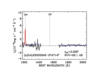
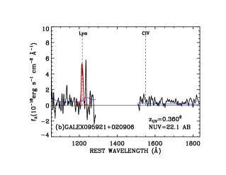
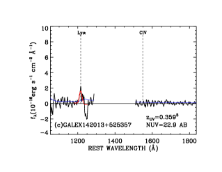
Figure 1.— (Top row) Examples of LAE UV spectra with the full range of assigned confidence classes (1=good, 2=marginal, 3=poor) indicated by superscripts to the listed Ly$\alpha$ redshifts. The Ly$\alpha$ redshift and the Ly$\alpha$ flux are measured from the Gaussian fit (red profile). We indicate the 1$\sigma$ noise array with the blue line. Each UV spectrum consists of the GALEX FUV spectral band, a band gap, and the GALEX NUV spectral band. We examine the UV spectra for high-excitation lines like CIV to help identify AGNs. (Bottom row) Below each UV spectrum, we show the corresponding optical spectrum. The three example LAEs were also selected to illustrate the quality of the optical spectra obtained from different telescopes/instruments. The archival VLT/VIMOS spectrum is from zCOSMOS (Lilly et al., 2007). We use these optical spectra to confirm our LAE candidates and to help identify AGNs via the BPT diagnostic diagram.

(A color version of this figure is available in the online journal.)

In Barger et al. (2012), we describe in detail our method to convert multiple GALEX low-resolution slitless spectroscopic images into a three-dimensional (two spatial axes and one wavelength axis) data cube. Here, we provide a brief overview of this process. For each of our four fields, we begin our data cube construction with archival 1.25 degree diameter FUV grism intensity maps. For each intensity map, we know the wavelength dispersion and the dispersion direction, and this allows us to extract a spectrum for each spatial position thus forming an initial data cube. A data cube constructed from a single slitless spectroscopic image will suffer from overlapping spectra caused by neighboring objects that are oriented in-line with the dispersion direction. However, the spectral dispersion direction can be altered from one exposure to the next by changing the grism rotation angle, and objects that overlap in one rotation angle are unlikely to overlap in another rotation angle. Thus, we are able to disentangle overlaps by requiring our selected fields to have hundreds of exposures with a corresponding number of rotation angles.

For each field, we construct hundreds of data cubes - one for each exposure - and then combine these initial data cubes applying a 5$\sigma$ cut to remove contamination from overlapping sources. This results in an intermediate data cube that has a wavelength step of 2.5 Å and a wavelength range of $1345$ to $1795$ Å. We resample this intermediate cube to form wavelength slices with a 10 Å wavelength extent sampled every 5 Å. We designed the wavelength slices to have a wavelength extent that matches the spectral resolution of GALEX. To account for emission line objects that would otherwise be split into two adjacent wavelength slices, we decided to make wavelength slices every 5 Å interval. For each slice, we subtracted the average of independent slices on either side of the primary slice, N. We used slices N-10, N-8, N-6 and slices N+6, N+8, and N+10 to form this average. This procedure subtracts most of the background residual structure and most of the continuum from objects within the data cube.

The final background subtracted FUV data cubes have a 50^′ diameter field of view and cover a wavelength range of 1395 to 1745 Å or a Ly$\alpha$ redshift range of $z=$ 0.15 to 0.44. For each wavelength slice, we used SExtractor (Bertin & Arnouts, 1996) to identify all 4$\sigma$ sources within the cube and then visually inspected each source and its spectrum (1-D and 2-D) to eliminate objects that were artifacts. During this visual inspection, we assigned a confidence category ($1=$ good, $2=$ fair, $3=$ uncertain) reflecting our confidence that the identified candidate is real and not an artifact. We applied this data cube search method and found 62 CDFS, 51 GROTH, 22 NGPDWS, and 38 COSMOS candidate LAEs (see Table 1). In Figure 1(a), (b), and (c), we show extracted 1D spectra for all confidence categories to illustrate the quality of our GALEX spectra. We estimate spectral noise by examining regions above and below the object’s two-dimensional spectrum. In general, spectral noise will increase as contamination from neighboring sources increases and as the spectral response falls off toward the edges of the spectral window. As in Barger et al. (2012) and Wold et al. (2014), we use our modified version of the GALEX pipeline software to extract two and one-dimensional spectra rather than extracting spectra directly from our data cubes. Our modified method uses profile-weighted spectral extraction (Horne, 1986) which provides modest improvement to the spectral signal to noise. Additionally, our modified extraction method, which is optimized to extract a single spectrum, provides a check on our LAE candidate sample which is selected based on a search of our four data cubes.

3.2. Optical Spectroscopic Follow-up

We used optical spectroscopic follow-up to confirm the veracity of our candidate LAEs and to identify optical AGNs. For our sample of 173 candidate LAEs, we obtained optical spectroscopic information for 171. To populate our optical spectroscopic target list, we visually identified the closest optical counterpart to the LAE candidate’s position in the FUV image which has a spatial resolution of $\sim 5^{\prime\prime}$. Follow-up spectroscopic observations were primarily obtained with the Hydra fiber spectrograph on the Wisconsin–Indiana–Yale–NOAO (WIYN) telescope. Each WIYN target was observed for a total of $\sim 3$ hours in a series of runs from January to March 2016. We configured the spectrograph using the “red” fiber bundle and the 316@7.0 grating at first order with the GG-420 filter to provide a spectral window of $\sim$4500–9500 Å with a pixel scale of 2.6 Å per pixel. The Hydra “red” fibers are 2^′′ diameter and have a positional accuracy of 0.3^′′, which ensured that the majority of light from our target galaxies was observed with little contamination from the sky and neighboring sources. We employed the IRAF task dohydra in the reduction of our spectra. This task is specifically designed for reduction of data from the Hydra spectrograph and includes steps for dark and bias subtraction, flat fielding, dispersion calibration, and sky subtraction. In Figure 1(f), we show an example of a WIYN/HYDRA obtained spectrum.

We also targeted a subset of LAE candidates with the DEep Imaging Multi-Object Spectrograph (DEIMOS; Faber et al., 2003) on Keck II. The observations were made with the ZD600 line mm^-1 grating blazed at 7500 Å. This gives a resolution of $\sim$ 5 Å  with a 1^′′ slit and a wavelength coverage of 5300 Å. Each $\sim$30 minute exposure was broken into three subsets, with the objects stepped along the slit by 1.5^′′ in each direction. The raw two-dimensional spectra were reduced and extracted using the procedure described in Cowie et al. (1996). In Figure 1(d), we show an example of a Keck/DEIMOS spectrum.

Our optical follow-up with WIYN and Keck was designed to have sufficient signal-to-noise to place our sources on the BPT diagnostic diagram (Baldwin et al., 1981, see Section 3.6). Thus, our optical spectra typically displayed easily identifiable H$\alpha$ and [OIII] emission lines. In all cases, at least two spectroscopic lines were required to measure the optical redshift. From our observed Keck spectra, we find that our LAEs have a median H$\alpha$ line flux of $9\times 10^{-16}$ erg s^-1cm^-2 giving an uncorrected-for-dust SFR of 2 M_⊙ yr^-1 at $z=0.3$. From our shallower WIYN spectra, we estimate any H$\alpha$ line with a flux greater than $2\times 10^{-16}$ erg s^-1cm^-2 will be detected at the 5$\sigma$ level. Thus, we do not expect any significant confirmation bias to be introduced by optically following-up our candidates with two different telescopes. In Section 3.5, we show that the vast majority of LAE candidates without a recovered optical redshift are assigned the lowest confidence category, and we argue that as a general rule increasing the depth of our optical spectra would only serve to further follow-up spurious LAE candidates.

When a LAE candidate’s optical counterpart was found to have an existing archival optical redshift, we relied on the archival data to confirm our proposed Ly$\alpha$ based redshift. This practice reduces the need for telescope time and should not impose a significant sample selection bias since (in all but two cases) we have targeted the non-archival sources with WIYN or Keck. We used archival VLT/VIMOS redshifts and spectra from the zCOSMOS survey (for COSMOS; Lilly et al., 2007) and from the VIMOS VLT Deep Survey (for CDFS; Le Fèvre et al., 2013). In Figure 1(e), we show an example of the archival VLT/VIMOS spectra. For 23 LAE candidates, their published optical redshifts lack accompanying optical spectra. These optical redshifts allow us to confirm the veracity of 19 candidates and falsify 4 candidates, but we are unable to examine their optical spectra for AGN features. In one case, GALEX033150-280811, there is a published optical spectroscopic AGN classification (Mao et al., 2012), and we use this classification in our study. They find that this object has emission line ratios typical of AGN activity, which is broadly consistent with one of our optical AGN classes. In Section 3.6, we discuss our AGN classification scheme in more detail.

3.3. Catalog Completeness

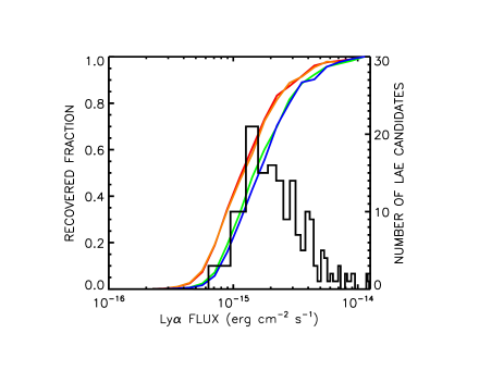
Figure 2.— Fraction of simulated Ly$\alpha$ emitters recovered as a function of the emission-line flux. The red, orange, green, and blue curves show recovered fractions from the CDFS, GROTH, NGPDWS, and COSMOS fields, respectively (also see Table 1). The histogram shows the number of LAE candidates as a function of flux for all four GALEX fields.

(A color version of this figure is available in the online journal.)

To determine the limitations of our multi-field catalogs and to compute the LAE galaxy LF, we measured our ability to recover fake emitters as a function of flux. For each field, we added 1000 simulated emitters uniformly within the field’s data cube. We did not model morphology or size difference, since nearly all emitters are unresolved at the spatial ($\sim 5^{\prime\prime}$) and spectral resolution ($\sim 10$ Å) of the GALEX grism data. We then ran our standard selection procedure and found the number of recovered objects. We independently performed the above procedure ten times, giving a total of 10,000 input sources. In Table 1, we list the flux threshold above which each field is greater than 50$\%$ complete. As expected, the completeness limit scales as the inverse square root of the exposure time. In Figure 2, we show the completeness as a function of the emission-line flux. The black histogram displays the Ly$\alpha$ flux distribution of our 173 LAE candidates.

3.4. Catalogs of LAE Candidates by Field

In Tables 4-7, we list all of the LAE candidates in the CDFS (Table 4), GROTH (Table 5), NGPDWS (Table 6), and COSMOS (Table 7) fields ordered by right ascension. We measured FUV and NUV AB magnitudes from the archival GALEX background subtracted intensity maps (Morrissey et al., 2007). We first determined the magnitudes within 8^′′ diameter apertures centered on each of the emitter positions. To correct for flux that falls outside our apertures, we measured the offset between 8^′′ aperture magnitudes and GALEX pipeline total magnitudes for all bright cataloged objects (20-23 mag range) within our fields. We determined the median offset for each field (typically $\sim 0.5$ mag) and applied these to our aperture magnitudes. For extended sources we adopt the GALEX cataloged magnitude which uses SExtractor’s AUTO aperture. We list these magnitudes in Tables 4-7.

We corrected our one-dimensional FUV spectra for Galactic extinction assuming a Fitzpatrick (1999) reddening law with R_V=3.1. We obtained $A_{V}$ values from the Schlafly & Finkbeiner (2011) recalibration of the Cardelli et al. (1989) extinction map as listed in the NASA/IPAC Extragalactic Database (NED). Galactic extinction increases the Ly$\alpha$ flux by $\sim$11% for the COSMOS LAEs, $\sim$4% for the GROTH LAEs, and $\sim$6% for the CDFS and NGPDWS LAEs.

From these extinction corrected spectra, we measured the redshifts, the Ly$\alpha$ fluxes, and the line widths using a two step process. First, we fit a 140 Å  rest-frame region around the Ly$\alpha$ line with a Gaussian and a sloped continuum (e.g., see Figure 1(a), (b), and (c)). A downhill simplex optimization routine was used to $\chi^{2}$ fit the five free parameters (continuum level and slope plus Gaussian center, width, and area). We used the results of this fitting process to subtract the continuum and as a starting point for the second step. In the second step, we used the IDL MPFIT procedures of Markwardt (2009) to $\chi^{2}$ fit the remaining three Gaussian parameters. We found that this two step procedure rather than a 5 parameter MPFIT solution resulted better $\chi^{2}$ fits. With the best-fit redshifts and Ly$\alpha$ fluxes, we calculated Ly$\alpha$ luminosities. When available, we used the more precise optical redshift rather than the Ly$\alpha$ redshift to calculate the Ly$\alpha$ luminosities. We list the Ly$\alpha$ redshifts and luminosities in Tables 4-7. During the initial visual inspection of the 1-D and 2-D spectra, we classified our LAE candidates into three qualitative categories ($1=$good, $2=$fair, $3=$uncertain) reflecting our confidence that the identified candidate is real and not an artifact. Our LAE detection confidence is given in Tables 4-7 as superscripts to the Ly$\alpha$ redshift.

The rest-frame EW_r(Ly$\alpha$) measured on the spectra are quite uncertain due to the very faint UV continuum. We obtained a more accurate rest-frame EW by dividing the measured Ly$\alpha$ flux by the continuum flux measured from the broadband FUV image (corrected for the emission-line contribution). We computed the EW uncertainty by propagating the 1$\sigma$ error from our FUV and Ly$\alpha$ flux measurements. It is these rest-frame EWs with 1$\sigma$ errors that are listed in Tables 4-7. In Section 4, we use these measurements to construct the $z\sim 0.3$ rest-frame EW distribution for star-forming LAEs.

Candidate X-ray counterparts were identified by matching all X-ray sources within a $6^{\prime\prime}$ radius from the data cube position. We then manually inspected the matches to reject false counterparts caused by X-ray sources with an optical counterpart neighboring but not associated with the LAE in question. We list the Chandra X-ray luminosity of each identified counterpart in Tables 4-7. LAE candidates within the X-ray footprint that lack detections were given X-ray luminosities of ‘-999’. At our survey’s redshift of $z\sim 0.3$, the X-ray imaging depth ($f_{2-8,10,10{\rm\,{keV}}}\sim 6.7$, $3.8$, $8.9\times 10^{-16}$ erg cm^-2 s^-1) corresponds to an X-ray luminosity of $\sim 10^{41}$ erg s^-1 for our CDFS, GROTH and COSMOS fields (Lehmer et al., 2005; Laird et al., 2009; Civano et al., 2016). The X-ray imaging depth for the NGPDWS field ($f_{2-7\,{\rm{keV}}}\sim 1.5\times 10^{-16}$ erg cm^-2 s^-1) corresponds to an X-ray luminosity of $\sim 10^{42}$ erg s^-1 (Kenter et al., 2005). For the central 484.2 arcmin² of the CDFS, we use a deeper X-ray imaging survey that has a sensitivity limit ($f_{2-7\,{\rm{keV}}}\sim 2.7\times 10^{-17}$ erg cm^-2 s^-1) that corresponds to an X-ray luminosity of $\sim 10^{40}$ erg s^-1 (Luo et al., 2017).

In the final column of Tables 4-7, we give an AGN classification. Our AGN classification scheme is described in Section 3.6.

3.5. Spurious LAE Candidates

We obtained optical redshifts and spectra from archival sources and combined this with our own optical spectra from Keck-DEIMOS and WIYN-Hydra (see Section 3.2). For our sample of 173 candidate LAEs, we have optical spectroscopic information for 171. Using these data, we found that 27 LAE candidates are spurious. These spurious sources have optical redshifts that are not consistent with the redshifts derived from the candidate Ly$\alpha$ emission line ($z_{UV}$) or have no viable optical counterpart. Specifically, we consider any source with an optical redshift outside of $z_{UV}\pm 0.03$ to be spurious. We found that two of our spurious LAE candidates are known X-ray bright stars. Both stars are relatively high confidence candidates (given 1 and 2 confidence classifications) and were selected based on emission at an observed wavelength of $1550$ Å indicating C IV $\lambda 1549$ emission. We are confident that these are C IV $\lambda 1549$ selected because both stars display Mg II $\lambda 2798$ emission in their GALEX NUV spectrum. We also found two O VI $\lambda 1035$ selected AGNs (GALEX142010+524029 and 143554+351910) at $z\sim 0.55$. For these two high-redshift interlopers, Ly$\alpha$ emission falls in the gap between the GALEX FUV and NUV bands. For both sources, strong C IV $\lambda 1549$ emission is observed in the NUV spectrum. Overall, our optical spectroscopic follow up indicates that our data cube search selects real emission line objects (Ly$\alpha$, C IV, and O VI emitters) 87% of the time or 148 confirmed sources out of a total of 171 candidates. For the purposes of this study, we consider any non-Ly$\alpha$ selected source to be spurious.

In Tables 4-7, we indicate spurious objects with optical redshifts not consistent with their Ly$\alpha$ redshifts by showing their optical redshift in parentheses. We indicate stars by setting their optical redshift to ‘star’ in Column 14. Additionally, we targeted 8 candidate LAEs with WIYN but did not recover an optical redshift. We indicate these objects by setting their optical redshifts to ‘no z’ in Column 14. All spurious LAE candidates are given blank entries for the Ly$\alpha$ luminosity and the rest-frame EW_r(Ly$\alpha$) fields in Columns 8 and 9.

Given the $\sim 5^{\prime\prime}$ spatial resolution of GALEX, it is possible that some of the spurious LAE candidates result from closely paired systems in which we have inadvertently targeted the wrong optical counterpart. To investigate this possibility, we examine the available optical images and find that the majority ($55\%$) of candidates have alternative optical counterparts within $5^{\prime\prime}$. However, the centroid of the GALEX source can typically be determined with an accuracy much less than $5^{\prime\prime}$, and we know that $87\%$ of our candidates are confirmed with optical spectra. Thus, we suspect that the importance of inadvertently targeting the wrong optical counterpart can be better assessed by computing our confirmation rate of high confidence candidates. As discussed in Section 3.1, during our initial data cube search we visually inspected each GALEX spectrum (1-D and 2-D) and assigned a confidence category ($1=$ good, $2=$ fair, $3=$ uncertain) reflecting our confidence that the identified candidate is real and not an artifact. Candidates with higher confidence measures (1 or 2) are optically confirmed $98\%$ percent of the time, or 116 out of a total of 118. On the other hand, candidates with low confidence measures (3) are optically confirmed $60\%$ percent of the time, or 32 out of a total of 53. Applying the high confidence percentage to our total sample size, we estimate that $\sim 3$ spurious LAE candidates could result from closely paired systems in which we have inadvertently targeted the wrong optical counterpart. Given this low estimate, we make no attempt to correct for this effect, and we simply exclude all spurious candidates from further analysis.

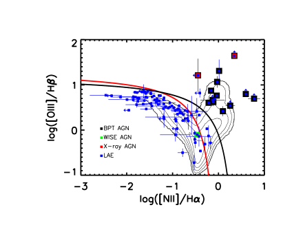
Figure 3.— BPT diagram for our LAE sample with narrow emission line optical spectra. The black curve shows the theoretical separation between AGNs and star-forming galaxies proposed by Kewley et al. (2001). The red curve shows the empirical separation between SDSS AGNs and star-forming galaxies proposed by Kauffmann et al. (2003). For the purposes of our study we require BPT AGNs to lie to the upper-right of both curves (see Section 3.6 for details). We show narrow-line X-ray AGNs which are LAEs with X-ray luminosities greater than $10^{42}$ erg s^-1 (red squares). We also indicate a WISE AGN which is identified via the color cut prescribed by Assef et al. (2013, green square). The black contours show the distribution of SDSS sources on a log scale.

(A color version of this figure is available in the online journal.)

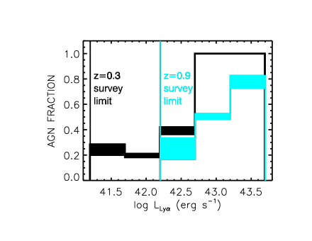
Figure 4.— AGN fraction per Ly$\alpha$ luminosity bin for both the $z=0.3$ (black histogram) and $z=0.9$ (cyan histogram; Wold et al., 2014) EW $>20$ Å LAE samples. The filled histogram regions show the boost in the AGN fractions caused by restricting the survey to areas with deep X-ray data. This restriction ensures a robust AGN classification at the expense of sample size. We show the approximate luminosity limit for each LAE survey with vertical black and cyan lines. In all observed $0.5$ dex Ly$\alpha$ luminosity bins, we find AGN fractions that are $\sim 20\%$ or greater.

(A color version of this figure is available in the online journal.)

3.6. AGN - Galaxy Identification

We made a classification of whether an emitter was an AGN based on: X-ray imaging, UV spectra, optical spectra, and infrared imaging. We classified objects as X-ray AGNs (denoted by ‘x’ in Tables 4-7 Column 15) if their X-ray luminosity exceeded $10^{42}$ erg s^-1 (e.g., see Hornschemeier et al., 2001; Barger et al., 2002; Szokoly et al., 2004). We note that archival X-ray imaging is available for $75\%$ percent of our survey area, and deep X-ray imaging that has a depth better than $1\times 10^{-15}$ erg cm^-2 s^-1 is available for $49\%$ percent of our survey area. We classified objects as UV AGNs (denoted by ‘u’ in Tables 4-7 Column 15) by examining the GALEX spectra for high-excitation lines such as C IV $\lambda 1549$ (for details on this procedure see Cowie et al., 2010, 2011). We note that this does not provide a uniform AGN diagnostic because in some cases the gap between the FUV and NUV bands prevents the observation of potential high excitation UV lines (e.g., see Figure 1(a)). We classified objects as WISE AGNs (denoted by ‘w’ in Tables 4-7 Column 15) via the color cut as prescribed by Assef et al. (2013). Finally, we classified objects as optical AGNs based on emission line ratios via the BPT diagnostic diagram (Baldwin et al., 1981) or the presence of broad emission lines ($\gtrsim 1000$ km s^-1 denoted by ‘n’ or ‘b’, respectively in Tables 4-7 Column 15).

In Figure 3, we show a BPT diagram of [OIII]$\lambda 5007/$H$\beta$ versus [NII]$\lambda 6584$/H$\alpha$ for our sample of LAEs with narrow emission line optical spectra. The BPT diagram uses the ratio of neighboring emission lines which are insensitive to flux calibration and reddening effects to separate star-forming (SF) galaxies from AGNs. The red curve shows the empirical separation between SDSS AGNs and SFs proposed by Kauffmann et al. (2003). The black curve shows the theoretical separation between AGNs and SFs proposed by Kewley et al. (2001). Objects that lie in between these two curves are generally classified as intermediate objects with both AGN and SF contributions. For our study, we require a BPT AGN to be positioned above or to the right of both curves. As a reference we show contours representing the distribution of sources from the Sloan Digital Sky Survey (SDSS; York et al., 2000) on a log scale. We have taken emission line measurements from the MPA-JHU catalog for SDSS DR7.

We restricted our BPT sample to sources with either H$\alpha$ or [OIII]$\lambda 5007$ detected with a signal-to-noise above 4. Objects with [NII]$\lambda 6584$ or H$\beta$ detected with a signal-to-noise below 1, have their flux values set to 1$\sigma$ and are displayed as upper or lower limits, respectively. In Figure 3, the 13 LAEs identified as BPT AGNs are outlined in black. Two of these BPT AGNs are also identified as X-ray AGNs (red outlined symbols). We find one WISE AGN that is not identified as a BPT AGN (green outlined symbol). For our sample of LAEs, all UV AGNs are also found to be broad-line AGNs (BLAGNs; note only narrow-emission line objects are shown in Figure 3). Overall, we find that 37 out of our 146 non-spurious LAEs are classified as AGNs by some means. As described in the next section, we classify optical absorber LAEs as AGNs, and we include these objects in our total AGN count of 37.

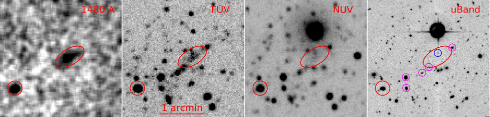
Figure 5.— Images of the extended LAE candidate GALEX033145-281038 with $z_{UV}=0.218$ (red ellipse). From left to right, we show a 1480Å data cube slice with a width of 10Å, the GALEX FUV band ($\Delta\lambda=$ 1344-1786 Å), the GALEX NUV band ($\Delta\lambda=$ 1771-2831 Å), and a CFHT u-band ($\Delta\lambda=$ 3400-4100 Å) image with a 5$\sigma$ depth of $\sim 26.5$ AB magnitude. The extended LAE has a major axis of about 23^′′ based on the FUV broad band image or $\sim$80 kpc at $z=0.218$. It has a $\sim$22 AB FUV counterpart but is very faint in the NUV and u-band. We highlight a nearby LAE, GALEX033150-281120, with $z_{UV}\sim z_{opt}=0.213$ (red $r=10^{\prime\prime}$ circle), five sources with known optical redshifts at $z\sim 0.215$ (magenta $r=5^{\prime\prime}$ circles), and a background source with an optical redshift of $z=0.387$ (blue $r=5^{\prime\prime}$ circle). We note that the wavelength range of FUV broadband image encompasses the wavelength of the proposed extended Ly$\alpha$ emission. In the FUV image, we indicate the angular size of 1^′.

(A color version of this figure is available in the online journal.)

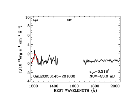
Figure 6.— The GALEX spectrum of the extended LAE candidate GALEX033145-281038. As in Figure 1, we show our Gaussian fit from which we measure the Ly$\alpha$ redshift and the Ly$\alpha$ flux (red profile). This source was not discovered in previous GALEX studies because of their requirement for all objects to have a bright NUV continuum (NUV$<22$).

(A color version of this figure is available in the online journal.)

Figure 7.— Optical spectra for three LAEs with weak optical emission lines, referred to as absorber LAEs. Ly$\alpha$ emission requires a source of relatively hard ionizing radiation and, as discussed in Section 3.7, we suspect that these objects are obscured AGNs with favorable geometry and/or kinematics that allows for the escape of Ly$\alpha$ photons.

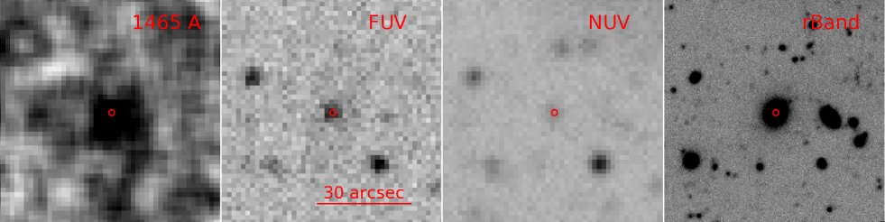
Figure 8.— Images of the absorber LAE GALEX143613+344813 with $z_{UV}\sim z_{opt}=0.204$. From left to right, we show a 1465Å data cube slice with a width of 10Å, the GALEX FUV band ($\Delta\lambda=$ 1344-1786 Å), the GALEX NUV band ($\Delta\lambda=$ 1771-2831 Å), and a KPNO Mayall 4m telescope/MOSAIC r-band ($\Delta\lambda=$ 5700-7000 Å) image with a 5$\sigma$ depth of $\sim 26$ AB magnitude. We obtained an optical spectrum with WIYN/HYDRA. We indicate the $r=1^{\prime\prime}$ WIYN/HYDRA fiber position with a red circle. The resulting spectrum is shown in Figure 7(b). We argue that the source targeted by WIYN is the only viable target and this suggests that - at least in some cases - our absorber LAEs are not closely paired systems in which we have inadvertently targeted the wrong optical counterpart. In the FUV image, we indicate the angular size of 30^′′.

(A color version of this figure is available in the online journal.)

Previous $z=0.3$ studies based on the GALEX pipeline reductions have estimated a wide range AGN contribution to the FUV LAE sample. These AGN fraction estimates have ranged from approximately 15 to 45$\%$ (Finkelstein et al., 2009b; Cowie et al., 2011). Our AGN contribution estimate for our EW $>20$ Å LAE sample is 26 $\pm$ 5$\%$, or 22 $\pm$ 5 $\%$ if absorber LAEs are not included in the AGN count. We apply the EW cut to be consistent with high-redshift LAEs samples which typically use this constraint to remove low-redshift interlopers such as [OII] emitters. If we limit our sample to EW $>20$ Å LAEs previously discovered in the GALEX pipeline reductions, then we find an AGN fraction of $\sim 34\%$. We note that the AGN fraction is not an invariant property of LAE samples. As previously pointed out by Nilsson & Møller (2011), Wold et al. (2014), and discussed in Section 5, the AGN fraction is strongly dependent on the sample’s Ly$\alpha$ luminosity range, such that - holding everything else constant - samples probing more luminous LAEs will have higher AGN fractions. In Figure 4, we show how the AGN fraction increases with Ly$\alpha$ luminosity in both the $z=0.3$ and $z=0.9$ EW $>20$ Å LAE samples. For this Figure, we have counted the $z=0.3$ absorber LAEs as AGNs. In all observed $0.5$ dex Ly$\alpha$ luminosity bins, we find AGN fractions that are $\sim 20\%$ or greater. At a given Ly$\alpha$ luminosity the $z=0.3$ sample has a higher AGN fraction. This can be attributed to the strong luminosity boost from $z=0.3$ to $0.9$ observed in the typical LAE galaxy (discussed further in Section 6).

Previous studies have shown that in order to achieve a complete consensus of AGNs, multi-wavelength datasets are required (e.g., Hickox et al., 2009). Thus, our primary reason for using X-ray imaging, UV spectra, optical spectra, and infrared imaging to identify AGNs is to increase the completeness of our AGN sample. The other reason we use multiple identification methods is because we lack uniform coverage for any one method. We lack deep X-ray imaging for $49\%$ of our survey. Depending on the LAE’s redshift, the GALEX band gap between FUV and NUV bands may prevent us from observing high-excitation lines in the UV spectrum. While we have optical redshifts for all but two of our LAEs, we only have optical spectra for $86\%$ of our LAE sample (archival redshifts are more readily available than archival spectra). We have infrared imaging for all fields via the all sky WISE survey, but the depth of this survey depends strongly on ecliptic latitude. By using our multi-wavelength data, we ensure that every LAE is classified by at least two methods. While utilizing all methods clearly provides advantages, we may also be reducing the reliability of our AGN sample. For example, Assef et al. (2013) estimate that their prescribed WISE color selection reliably identifies AGNs 90% of the time.

We assess the importance of these completeness and purity concerns by limiting our survey to regions with deep X-ray imaging. X-ray selection provides a robust AGN identification which is often used as the base-line truth in studies that compare AGN classification methods (e.g., Trouille & Barger, 2010). Furthermore, by limiting our survey to regions with deep X-ray imaging, we ensure that every LAE is classified by at least three methods. We compare results derived from our full sample to results computed from our X-ray covered sample to assess any significant incompleteness in our AGN sample. Additionally, within the deep X-ray fields, we find that all UV and WISE AGNs are independently classified as X-ray AGNs. Falsely identified AGN in one method are unlikely to be falsely identified in another method. Thus, concerns about the purity of the WISE and UV selected AGNs should be eased. We note that within the deep X-ray fields 8 optically identified AGN are not identified as X-ray AGN. Three of these eight are $10^{41}$erg s^-1 X-ray sources, perhaps indicating that our straight $10^{42}$ erg s^-1 luminosity cut is missing some X-ray faint AGN. The remaining 5 optical only AGNs are composed of two ‘absorbers’ (see 3.7) and three BPT AGNs. These could indicate falsely identified optical AGNs or represent a population of heavily obscured AGNs.

While the comparison of our full sample to our X-ray deep sample does not completely alleviate all completeness and purity concerns, it does significantly improve our AGN classification and allows us to assess any effect on our main results. Furthermore, in Section 5, we consider a method to measure the LAE luminosity function without AGN identification. Here we simultaneously fit the combined SF+AGN LF with a Schechter + power-law function. This bypasses AGN identification concerns at the expense of having to assume a functional form to the AGN luminosity function. In Section 5, we show that restricting the survey’s area to deep X-ray fields or simultaneously fitting the combined SF+AGN LF does not significantly change our LAE luminosity function results.

3.7. Extended and Absorber LAE Candidates

We found one highly extended Ly$\alpha$ source, LAE candidate GALEX033145-281038 with $z_{UV}=0.218$. In Figure 5, we show this candidate in a 1480A data cube slice with a width of 10A, the GALEX FUV band ($\Delta\lambda=$ 1344-1786 Å), the GALEX NUV band ($\Delta\lambda=$ 1771-2831 Å), and a CFHT u-band ($\Delta\lambda=$ 3400-4100 Å) image with a 5$\sigma$ depth of $\sim$26.5 AB magnitude. In Figure 6, we show our exacted 1-D GALEX spectrum for this object. With a measured FUV major axis of 0.37^′ or 80 kpc at $z=0.218$ and a Ly$\alpha$ luminosity of $7.8\times 10^{41}$ erg s^-1, this extended source falls below the typical high-redshift Ly$\alpha$ blob physical extent ($\sim 100$ kpc) and Ly$\alpha$ luminosity ($\sim 10^{43}$ erg s^-1). It has a 22 AB FUV counterpart but is very faint in the NUV and u-band. In Figure 5, we highlight a nearby LAE, GALEX033150-281120, with $z_{UV}\sim z_{opt}=0.213$ (red $r=10^{\prime\prime}$ circle), five sources with known optical redshifts at $z\sim 0.215$ (magenta $r=5^{\prime\prime}$ circles), and a background source with an optical redshift of $z=0.387$ (blue $r=5^{\prime\prime}$ circle). The closest object with known matching redshift ($z=0.216$) is about 60 kpc away from the centroid of the extended source (magenta circle to the south-east or lower-left relative to the extended LAE). The ECDFS X-ray field lies to the north of this source, and we lack X-ray data for this source or any of the potential counterparts.

While more data is needed to study this extended object, we note some similarities with more extensively studied spatially extended LAEs. In particular, the lack of a clear optical counterpart and the apparent over-density of nearby $z\sim 0.215$ sources is consistent with the properties of the Nilsson et al. (2006) Ly$\alpha$ nebula at $z=3.157$. The Nilsson et al. Ly$\alpha$ nebula has recently been re-examined by Prescott et al. (2015) with data from the Hubble Space Telescope and the Herschel Space Observatory. This object exists within a local over-density of galaxies and has no continuum source located within the nebula. Prescott et al. conclude that the Ly$\alpha$ nebula is likely powered by an obscured AGN located $\sim$30 kpc away. We also note that the only probable candidate found for the Barger et al. (2012) low-redshift ($z=0.977$) Ly$\alpha$ nebula was an AGN located 170 kpc away (Barger et al., 2012). Further advancing an AGN power source, Schirmer et al. (2016) have suggested that SDSS galaxies selected for their strong [OIII] emission lines and for their large spatial extent (Green Beans) are likely ionized by AGNs. Green Beans are estimated to be extremely rare ($\sim 3.3$ Gpc^-3) and to have very high Ly$\alpha$ luminosities ($\sim 10^{43}$ erg s^-1), so it is not clear that these objects are directly related to our relatively faint extended object found in a survey volume of $\sim 0.90\times 10^{6}$ Mpc³.

In Figure 7, we show 3 of the 6 LAEs with very weak optical emission lines. We refer to these LAEs as absorbers, and they are denoted with an ‘a’ in Column 15 in Tables 4-7. Given the poor resolution of GALEX, it is possible that absorbers are closely paired systems in which we have inadvertently targeted the wrong optical counterpart. In this scenario, the real LAE counterpart could still have an emission line optical spectrum. However, in Figure 8, we present our strongest case against this interpretation being true for all cases. For this LAE, the Ly$\alpha$ emission seen in the data cube slice has only one viable FUV counterpart which we targeted with WIYN/HYDRA (red circle indicates HYDRA’s $r=1^{\prime\prime}$ fiber location). The resulting optical spectra is shown in Figure 7(b). As might be expected from an absorber spectrum, the $r$-band morphology appears to be spheroidal. This LAE is within an X-ray imaging survey (Kenter et al., 2005) but is not detected. Based on the hard X-ray band detection limit, this absorber has an X-ray luminosity upper limit of $\sim 2\times 10^{42}$ erg s^-1. Four of the other absorbers, GALEX033145-274615, 033213-280405, 033251-280305, and 100010+015453, are also within X-ray surveys and are not detected in the hard X-ray band. This places an upper limit on their X-ray luminosities of $5\times 10^{39}$, $2\times 10^{41}$, $1\times 10^{41}$, and $2\times 10^{41}$ erg s^-1, respectively. We find that absorber GALEX033251-280305 is a soft X-ray source with a luminosity of $1\times 10^{41}$ erg s^-1 (Lehmer et al., 2005).

Another plausible explanation for an absorber LAE is that a faint star-forming galaxy responsible for the Ly$\alpha$ emission is out-shined in the optical by a superimposed absorber galaxy at the same redshift. In this scenario, even if we followup the correct optical counterpart, we would not recover the LAE’s uncontaminated optical spectrum.

We note that 4 out of 6 absorbers have blue FUV to NUV colors (FUV-NUV$<0$ ) and very large rest-frame EWs ($>200$ Å). While these objects lack a clear SF or AGN signature, we suggest that these objects are likely obscured AGNs with favorable geometry and/or kinematics that allows for the escape of Ly$\alpha$ photons.

Further evidence that heavily obscured AGNs can be strong Ly$\alpha$ emitters is demonstrated by our newly discovered data cube LAE GALEX095910+020732. This object was the focus of a multi-wavelength study that concluded that its nuclear emission must be suppressed by a N_H $\gtrsim 10^{25}$ cm^-2 column density (Lanzuisi et al., 2015). Unlike our absorber LAEs, this obscured object has strong optical emission lines including H$\alpha$. With our data cube search, we now know that this object is also a very luminous LAE with $L_{{\rm{Ly}\alpha}}=10^{42.7}$ erg s^-1. While this object did not meet our X-ray or infrared AGN criteria, we classified this object as a UV AGN based on a strong C IV emission line. For all six of our absorber LAEs, we find that C IV is not observable with the GALEX grism data because the emission line feature falls between the FUV and NUV bandpasses.

Throughout our subsequent analysis we classify these 6 absorber LAEs as AGNs. Furthermore, we exclude the extended LAE GALEX033145-281038 from both SF and AGN categories.

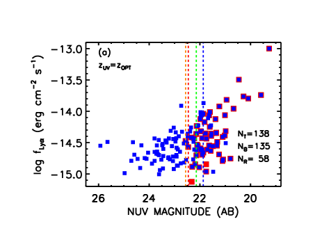
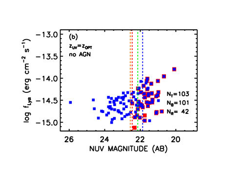
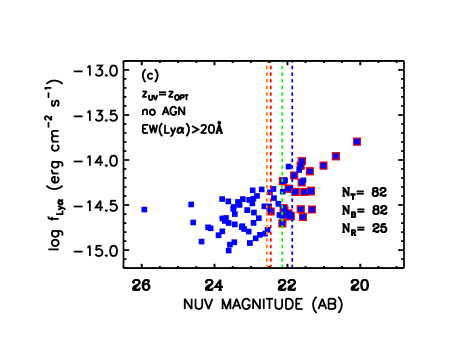
Figure 9.— (a) LAE NUV magnitude vs. Ly$\alpha$ flux for LAEs with optical redshifts that confirm their Ly$\alpha$ redshifts based on Ly$\alpha$ emission. Red squares show the pipeline LAEs found by Cowie et al. (2010, 2011) constrained to the data cubes’ 50^′ diameter FOVs. Blue squares show our data cube LAEs constrained to the pipeline’s redshift range ($z=0.195-0.44$). The dashed red, orange, green, and blue line shows the maximum NUV magnitude found in the pipeline sample for the CDFS, GROTH, NGPDWS, and COSMOS field, respectively. This roughly corresponds to the GALEX pipeline’s magnitude limit of NUV$\sim 22$. (b) The same as Figure 9(a), but with all AGNs removed. We note that many of the most luminous sources are removed by this cut. (c) The same as Figure 9(b), but with all EW_r(Ly$\alpha$)$<20$Å  objects removed. We note that the final sample contains $25$ pipeline LAEs. The data cube sample recovers all 25 of these objects plus 57 previously unidentified LAEs. In all panels, we indicate the number of data cube LAEs or blue squares (N_B), the number of pipeline LAEs or red squares (N_R), and the total number of LAEs (N_T).

(A color version of this figure is available in the online journal.)

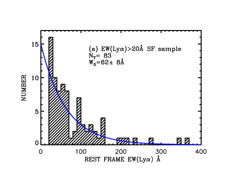
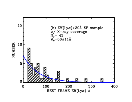
Figure 10.— (a) Ly$\alpha$ galaxy EW distribution. (b) Same as Figure 10(a), but with the LAE survey limited to regions with deep X-ray data to ensure a robust AGN classification. In each Figure, we indicate the best fit exponential (blue curve), the total number (N_T) of star-forming LAEs with EW $>20$ Å  used to compute the distribution and the EW distribution scale length (W₀).

(A color version of this figure is available in the online journal.)

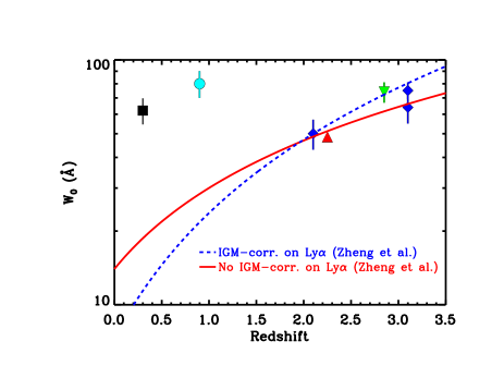
Figure 11.— Rest-frame EW scale lengths from our $z\sim 0.3$ sample (black square), the $z\sim 0.9$ Wold et al. (2014) sample (cyan circle), the $z=2.25$ Nilsson et al. (2009) sample (red upward triangle), the $z=2.1$ Guaita et al. (2010), $z=3.1$ Gronwall et al. (2007), and $z=3.1$ Ciardullo et al. (2012) samples (blue diamonds; values quoted from Ciardullo et al.), and $z\sim 2.85$ Blanc et al. (2011) sample (green downward triangle) vs. redshift. The dashed blue and solid red curves indicate the empirical EW scale length evolution with and without IGM absorption to the Ly$\alpha$ line flux, respectively, proposed by Zheng et al. (2014). In contrast to these previously suggested evolutionary trends, our new $z=0.3$ result plus our recent $z=0.9$ result favors a relatively constant EW scale length from $z=0.3$ - $3$.

(A color version of this figure is available in the online journal.)

3.8. Comparison of the GALEX Data Cube Sample with the GALEX Pipeline Sample

In Figure 9, we compare our data cube sample (blue squares) to the pipeline sample (red squares) as presented in Cowie et al. (2010) and Cowie et al. (2011) for GALEX fields CDFS, GROTH, NGPDWS, and COSMOS constrained to the data cubes’ 50^′ diameter FOVs. We require the sources to have optical redshifts in agreement with their Ly$\alpha$ based redshifts, and we limit our sample in this comparison to LAEs with $z>0.195$ to be consistent with the pipeline sample. The dashed vertical lines indicate the pipeline’s NUV continuum thresholds. As expected, the pipeline begins to miss objects fainter than the pipeline’s extraction threshold of $\sim$22 AB magnitude. In Figure 9(a), we show that within the same FOV our sample contains 135 LAEs, while the pipeline sample contains 58 LAEs. We note that there are three low-EW LAEs detected in the pipeline but not found with our data cube search. These objects have relatively low Ly$\alpha$ flux measurements (ranging from 8$\times 10^{-16}$ to 4 $\times$ 10^-15 erg cm^-2 s^-1 ). We find that our recovered fraction of fake sources falls below $\sim$90% at 4$\times$10^-15 erg cm^-2 s^-1 and then quickly declines with a $\sim$30$\%$ recovery at 1 $\times$ 10^-15 erg cm^-2 s^-1. Thus, we suspect that the missed pipeline LAE are accounted for by the data cube’s flux limit. Regardless, the missed sources have low EWs ($<20$Å) and are thus excluded from our final sample used to compute the Ly$\alpha$ EW distribution and LF. In Figure 9(b), we remove all AGNs (see Section 3.6 for AGN classification) and show that our sample contains 101 SF LAEs, while the pipeline sample contains 42 SF LAEs. In Figure 9(c), we show that the data cube sample finds all pipeline EW(Ly$\alpha$)$>$20 Å  star-forming LAEs plus an additional 57 LAEs that fall below the pipeline’s continuum detection threshold.

3.9. EW and LF Sample Definition

For the 146 non-spurious sources, we have 144 (125) optical redshifts (spectra) that agree with our Ly$\alpha$ redshifts. We note that 19 LAEs with optical redshifts were obtained from archival sources (see Tables 4-7) that lacked published spectra. For our final SF LAE sample, we start from these 146 LAEs and require sources to not be identified as an AGN in any way, have EW(Ly$\alpha$) $\geq$ 20Å, have $z>0.195$, and be detected above the $50\%$ flux completeness threshold as determined from our Monte Carlo simulations. We require our LAEs to have $z>0.195$ to be consistent with previous studies (Cowie et al., 2010, 2011). This removes 6 LAEs with $0.15<z<0.195$ from our final sample. Our final SF sample which is used to derive the Ly$\alpha$ LF and EW distribution has a size of 83 objects. Of these 83 LAEs, we have optical redshifts (spectra) for 81 (71) objects. The two LAEs in our final sample without optical followup (GALEX033108-274214 and 033346-274736) are assigned a high LAE confidence classification of 2 and 1, respectively. We include these optically un-targeted LAEs because targeted high confidence (1 and 2) candidates are optically confirmed $98\%$ percent of the time.

We emphasize that previous $z\sim 0.3$ samples used to compute the Ly$\alpha$ LF were biased against high-EW objects and had a smaller sample size of SF LAEs (Deharveng et al., 2008; Cowie et al., 2010). For example, Cowie et al. (2010) derived the $z\sim 0.3$ LF from 41 star-forming LAEs with EW(Ly$\alpha$)$>$20 Å in nine GALEX fields. With only four fields we have obtained a sample of 83 SF LAEs. Most importantly, our sample is not pre-selected from continuum bright objects, which facilitates the comparison of our LAE sample to high-redshift samples.

4. Equivalent Width Distribution

The Ly$\alpha$ EW in the rest frame is the ratio of Ly$\alpha$ flux relative to the continuum flux density divided by ($1+z$). Galaxies with extremely high Ly$\alpha$ EWs are proposed sites of low metallicity starbursts (Schaerer, 2003; Tumlinson et al., 2003), and these extreme emitters may play an increasingly dominant role at higher redshifts. In line with these expectations, there are studies that find a shift toward lower EW objects at lower redshifts (e.g., Ciardullo et al., 2012; Zheng et al., 2014). However, these studies lack an unbiased low-redshift constraint. Previously, the $z\sim 0.3$ EW distribution was derived from the GALEX pipeline reductions and thus was biased against high-EW objects (as described in Section 5.4 of Cowie et al., 2010). With our data cube sample we remove this bias and make a valid comparison to high-redshift EW distributions.

In Figure 10(a), we show our $z\sim 0.3$ rest-frame EW distribution for all LAEs in our SF sample. To compare our EW distribution to previous studies, we fit it with an exponential and find a scale length of 62 $\pm$ $8$ Å. We compute a maximum likelihood estimate of the scale length and compute the 1$\sigma$ error using the parameterized bootstrap method. In Figure 10(b), we show our $z\sim 0.3$ rest-frame EW distribution for all LAEs in our SF sample that have available deep X-ray data. The deep X-ray data have a depth of $\sim 10^{41}$erg s^-1 at $z\sim 0.3$ and provide a uniform AGN diagnostic. We find that the computed scale length is not significantly altered by the requirement of a more strict AGN diagnostic.

In Figure 11, we show the redshift evolution of the EW scale length. The dashed blue and solid red curves indicate the empirical EW scale length evolution with and without IGM absorption to the Ly$\alpha$ line flux, respectively, proposed by Zheng et al. (2014). In contrast to these previously suggested evolutionary trends, our new $z=0.3$ result plus our recent $z=0.9$ result (Wold et al., 2014) favors a relatively constant EW scale length from $z=0.3$ - $3$, or roughly 8 Gyrs. Our measured large scale length is in sharp contrast to the biased $z\sim 0.3$ GALEX pipeline LAE sample, which has an EW scale length of 23.7 Å (Cowie et al., 2010). We note that Cowie et al. (2010) corrected their EW distribution for the pipeline sample’s incompleteness and found their corrected distribution to be well described by a EW scale length of 75 Å. This estimate is within 2$\sigma$ of our result.

In the pipeline sample, no LAE galaxies are found with an EW(Ly$\alpha$)$>$120 Å. In our final SF sample, we find 16 of these extreme EW LAEs. These extreme EW LAEs are of interest given the recent studies suggesting that high-EW LAEs are efficient emitters of ionizing photons and potential analogs of reionization-era galaxies (e.g., Erb et al., 2016; Trainor et al., 2016).

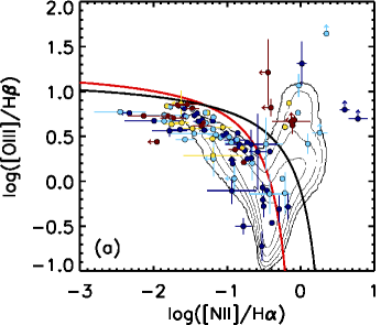
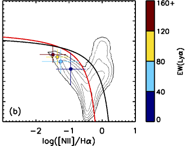
Figure 12.— (a) BPT diagram as presented in Figure 3 but with data points color-coded to indicate Ly$\alpha$ EWs. We note that star-forming LAEs with EW $>80$ Å  are only found in the upper left corner of the BPT diagram. (b) The average star-former [NII] to H$\alpha$ and [OIII] to H$\beta$ line ratios for each EW bin with error bars that indicate the standard deviation of the component data points. We find that the average high-EW LAE probes galaxies with more extreme ISM properties.

(A color version of this figure is available in the online journal.)

In Figure 12(a), we color-code our BPT diagram data (Figure 3) to show our Ly$\alpha$ EW measurements. We find that star-forming LAEs have a wide range of [NII] to H$\alpha$ and [OIII] to H$\beta$ line ratios, most likely indicating a wide range of ISM conditions. However, we note that LAEs with EW $>80$ Å  are only found in the upper left corner of the BPT diagram. This region is thought to be dominated by galaxies with lower metallicities, higher ionization parameters, and higher electron densities. To illustrate this trend more clearly, in Figure 12(b), we show the average star-former [NII] to H$\alpha$ and [OIII] to H$\beta$ line ratios for each of our adopted EW bins. The error bars show the standard deviation of the data points. We note that our observed trend, where high-EW LAEs preferentially occupy the upper left corner of the BPT diagram, is consistent with earlier $z=0.3$ results (Cowie et al. 2011; and see Trainor et al. 2016 for $z=2.5$ results). Cowie et al. compared LAEs to UV-selected galaxies (Ly$\alpha$ EW $\sim 0$ Å) and found that their $z\sim 0.3$ UV-selected galaxies were preferentially located in the lower right of the BPT diagram, roughly corresponding to our highest SDSS density contour shown in Figure 12, while their $z\sim 0.3$ LAEs were preferentially found in the upper left of the BPT diagram. Our results indicate that higher EW LAEs at $z=0.3$ on average probe galaxies with more extreme ISM properties and may offer promise as local analogs to high-redshift galaxies. We will further investigate the emission properties of the $z\sim 0.3$ LAE sample in a follow-up paper.

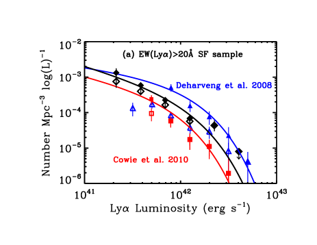
Figure 13.— (a) The SF Ly$\alpha$ LF at $z$ = 0.195-0.44 in deep GALEX grism fields with $EW(Ly\alpha)\geqslant 20$ Å(open diamonds–raw data; solid diamonds–corrected for the effects of incompleteness using the results from our Monte Carlo simulations). The black curve indicates the best-fit Schechter function to the SF data assuming a fixed slope of $\alpha=-1.75$. For comparison, we show raw and completeness corrected data from Deharveng et al. (2008, blue curve and triangle symbols) and Cowie et al. (2010, red curve and square symbols). (b) Same as Figure 13(a), but with the LAE survey limited to regions with deep X-ray data to ensure a robust AGN classification. We find that requiring a more robust AGN classification does not significantly alter our results derived from our full sample.

(A color version of this figure is available in the online journal.)

Figure 14.— The AGN Ly$\alpha$ LF at $z$ = 0.195-0.44 in deep GALEX grism fields with $EW(Ly\alpha)\geqslant 20$ Å(open stars–raw data; solid stars–corrected for the effects of incompleteness using the results from our Monte Carlo simulations). The black line indicates the best-fit power-law to the AGN data. Integrating over the observed luminosity range, we calculate the observed AGN Ly$\alpha$ luminosity density and find log $\rho_{Ly\alpha,AGN}^{obs}=38.1\pm 0.1$ erg s^-1Mpc^-3(from log $L=41.2$ to $43.7$) which is only 0.2 dex less than the observed SF Ly$\alpha$ luminosity density. We show our SF Ly$\alpha$ LF from Figure 13(a) for comparison.

Table 2Best-fit $z\sim 0.3$ Ly$\alpha$ Luminosity Function Parameters using a $\rho_{Ly\alpha}$ lower integration limit of log $L=41.2$.

Reference	$\alpha$	log $L^{\star}$	log $\phi^{\star}$	$\sigma$	log $\rho^{obs}_{Ly\alpha,SF}$	m	b	log $\rho^{obs}_{Ly\alpha,AGN}$
	(fixed)	(erg s-1)	(Mpc-3)		(erg s-1 Mpc-3)			(erg s-1 Mpc-3)
(1)	(2)	(3)	(4)	(5)	(6)	(7)	(8)	(9)
Deharveng et al. 2008	-1.35	42.0$\pm$0.1	-3.4$\pm$0.2	$\cdots$	38.6$\pm$0.2	$\cdots$	$\cdots$	$\cdots$
Cowie et al. 2010	-1.60	41.8$\pm$0.1	-3.8$\pm$0.1	$\cdots$	38.0$\pm$0.1	$\cdots$	$\cdots$	$\cdots$
This work (Best estimate)	-1.75	42.0$\pm$0.2	-3.7$\pm$0.3	$\cdots$	38.3$\pm$0.1	-2.0$\pm$0.3	38.6$\pm$12.4	38.1$\pm$0.1
This work (X-ray Covered)	-1.75	41.9$\pm$0.2	-3.6$\pm$0.4	$\cdots$	38.3$\pm$0.1	-2.4$\pm$0.2	55.1$\pm$8.6	38.1$\pm$0.1
This work (Schechter + fPL)	-1.75	41.9$\pm$0.2	-3.7$\pm$0.3	$\cdots$	38.3$\pm$0.1	-2.0(fixed)	38.8$\pm$0.2	38.2$\pm$0.2
This work (Schechter + PL)	-1.75	41.9$\pm$0.2	-3.7$\pm$0.3	$\cdots$	38.2$\pm$0.2	-2.1$\pm$0.6	43.0$\pm$24.3	38.3$\pm$0.2
This work (Saunders + fPL)	-1.75	41.2$\pm$1.6	-3.1$\pm$1.4	0.5$\pm$0.4	38.4$\pm$0.2	-2.0(fixed)	38.7$\pm$0.3	38.1$\pm$0.3
This work (Saunders + PL)	-1.75	41.3$\pm$1.2	-3.1$\pm$1.0	0.5$\pm$0.4	38.4$\pm$0.1	-1.7$\pm$0.4	25.5$\pm$17.0	38.0$\pm$0.4

Note. —

5. Luminosity Function

For the combined CDFS, GROTH, NGPDWS, and COSMOS fields, we compute the Ly$\alpha$ LF in the redshift range $z=0.195-0.44$ using the $1/V$ technique (Felten, 1976). The total area covered by our survey is 7423 arcmin² which indicates a Ly$\alpha$ survey volume of $0.90\times 10^{6}$ Mpc³. This is comparable to the largest LAE survey at $z=2.2$ which has a survey volume of $1.32\times 10^{6}$ Mpc³ (Konno et al., 2016) and is about 10 times smaller than the GALEX NUV LAE survey at $z=0.67-1.16$ which has a survey volume of $9.25\times 10^{6}$ Mpc³ (Wold et al., 2014). In Figure 13(a), we show our raw EW$({\rm{Ly}}\alpha)\geqslant 20$ Å star-forming Ly$\alpha$ LF with black open diamonds. We show the LF corrected for incompleteness using the results from our Monte Carlo simulations with solid symbols. Error bars are $\pm 1\sigma$ Poisson errors. We fit a Schechter function (Schechter, 1976) to the SF Ly$\alpha$ LF, where

$$\Phi_{SF}(L)dL=\phi^{\star}\left(\frac{L}{L^{\star}}\right)^{\alpha}e^{-(L/L^{\star})}d\left(\frac{L}{L^{\star}}\right).$$ (1)

For the Schechter function fit, we assume a fixed faint-end slope of $\alpha=-1.75$, which is the best-fit $z=2.2$ value found by Konno et al. (2016). This assumption is required because our $z\sim 0.3$ data lack the faint luminosity range necessary to constrain $\alpha$.

In Figure 13(b), we restrict our fields to regions with deep X-ray data and re-derive the star-forming Ly$\alpha$ LF. This removes the NGPDWS field and restricts the area of the remaining GALEX fields but ensures a uniform means of AGN classification (See Section 3.6). The X-ray imaging depth for our restricted field is $\sim 10^{41}$ erg s^-1 at $z\sim 0.3$, which is well below the $10^{42}$ erg s^-1 threshold typically used to identify AGN. Comparing this LF to the LF computed from the full LAE galaxy sample, we find that all star-forming LF points are consistent within 1$\sigma$ error bars. We find that requiring a more robust AGN classification does not significantly alter our results derived from our full sample.

In both panels of Figure 13, we compare our $z\sim 0.3$ LF to the results of two $z\sim 0.3$ Ly$\alpha$ LFs derived from GALEX pipeline data (Deharveng et al., 2008; Cowie et al., 2010, blue data and red data, respectively). Cowie et al. (2010) pointed out that all of their $z\sim 0.3$ raw Ly$\alpha$ LF measurements are comparable to the previously published raw LF determined by Deharveng et al. (2008). It is only after corrections for incompleteness are applied that the their results differ. Unlike the previous pipeline samples, our data cube LAE sample is not pre-selected from continuum bright objects and this greatly simplifies the estimation of corrections for incompleteness. With our larger and less biased sample, we find that our LF data points fall in between these two previous $z\sim 0.3$ LFs with best fit Schechter parameters summarized in Table 2.

Having identified the AGNs within our LAE sample, we may also compute the LF for Ly$\alpha$ emitting AGNs. In Figure 14, we show the AGN Ly$\alpha$ LF at $z$ = 0.195-0.44 in our survey fields with EW$({\rm{Ly}}\alpha)\geqslant 20$ Å(open stars–raw data; solid stars–corrected for the effects of incompleteness using the results from our Monte Carlo simulations). The black line indicates the best-fit power-law to the AGN data with the functional form:

$$\Phi_{AGN}(L)dL=10^{b}L^{m}dL.$$ (2)

The best-fit parameters are listed in Table 2.

To assess the amount of Ly$\alpha$ light emitted by star-formers and AGNs we calculate the observed Ly$\alpha$ luminosity density:

$$\rho_{Ly\alpha}^{obs}=\int L\Phi(L)dL,$$ (3)

and find log $\rho_{Ly\alpha,SF}^{obs}=38.3\pm 0.1$ (integrating over the luminosity range of log $L=41.2$ to infinity) and log $\rho_{Ly\alpha,AGN}^{obs}=38.1\pm 0.1$ erg s^-1Mpc^-3 (integrating over the survey’s luminosity range of log $L=41.2$ to $43.7$). This result indicates that AGNs are responsible for $\sim 39\%$ of the observed Ly$\alpha$ light at $z\sim 0.3$. We emphasize that this result is dependent on our survey’s luminosities limits. To estimate a lower limit to the AGN contribution, we integrate the SF LF from zero to infinity and compare this value to the $\rho_{Ly\alpha,AGN}^{obs}$. With these integration limits the luminosity density is simply

$$\rho_{{\rm{Ly}\alpha,}SF}^{total}=L^{\star}\phi^{\star}\Gamma(\alpha+2),$$ (4)

where $\Gamma$ is the Gamma function. Integrating down to zero makes our calculation more sensitive to the poorly constrained faint-end slope, but assuming reasonable $\alpha$ values we do not expect our total SF luminosity density calculations to be altered by more than a factor of 2. We find a total SF luminosity density of log $\rho_{Ly\alpha,SF}^{total}=38.8\pm 0.1$ erg s^-1Mpc^-3 which gives a lower-limit $z\sim 0.3$ AGN contribution of $17\%$. This significant AGN contribution emphasizes the need for caution when interpreting higher redshift LAE samples with limited or no AGN identification. We note that the assumed form of the AGN LF results in an AGN luminosity density that is very sensitive to the assumed upper integration limit. The assumed power-law LF is merely the simplest functional form given the observed Ly$\alpha$ luminosity range. This is also true for the assumed Schechter function since the SF LF must turn over at lower luminosities to prevent the total number of galaxies from diverging (for $\alpha\leq-1$).

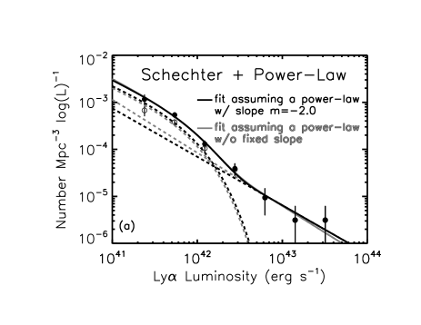
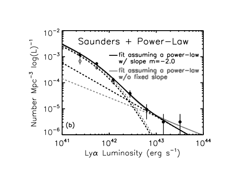
Figure 15.— (a) Combined SF and AGN Ly$\alpha$ LF at $z$ = 0.195-0.44 in deep GALEX grism fields with $EW(Ly\alpha)\geqslant 20$ Å(open circles–raw data; solid circles–corrected for the effects of incompleteness using the results from our Monte Carlo simulations). The black curve indicates the best-fit Schechter function $+$ power-law to the combined data assuming a Schechter fixed faint-end slope of $\alpha=-1.75$. The black dashed curve and line indicate the underlying best-fit Schechter function and power-law, respectively. The slope of the power-law has been fixed to the isolated best-fit value of -2.0 (see Figure 14 and Row 3 of Table 2). (b) Same as Figure 15(a), but with the data fit by a Saunders function $+$ power-law. Computing luminosity densities for both Schechter and Saunders fits, we find that the results agree within 1$\sigma$ errors. In both Figures, we also show the effect of allowing the power law slope to be a free parameter (grey dashed and solid curves). We find that this alteration does not significantly alter our computed luminosity densities. All results are summarized in Table 2.

Table 3Evolution of Ly$\alpha$ Luminosity Function Parameters assuming $\alpha=-1.75$ and a $\rho_{Ly\alpha}$ lower integration limit of log $L=41.41$.

Redshift	log $L^{\star}$	log $\phi^{\star}$	$\sigma$	log $\rho^{obs}_{Ly\alpha,SF}$	m	b	log $\rho^{obs}_{Ly\alpha,AGN}$	Reference
	(erg s-1)	(Mpc-3)		(erg s-1 Mpc-3)			(erg s-1 Mpc-3)
(1)	(2)	(3)	(4)	(5)	(6)	(7)	(8)	(9)
0.3	41.9$\pm$0.2	-3.7$\pm$0.3	$\cdots$	38.2$\pm$0.1	-2.0(fixed)	38.8$\pm$0.2	38.2$\pm$0.2	This work (Schechter + fPL)
0.3	41.9$\pm$0.2	-3.7$\pm$0.3	$\cdots$	38.1$\pm$0.2	-2.1$\pm$0.5	43.0$\pm$23.4	38.3$\pm$0.3	This work (Schechter + PL)
0.3	41.2$\pm$1.6	-3.1$\pm$1.6	0.5$\pm$0.4	38.2$\pm$1.4	-2.0(fixed)	38.7$\pm$0.7	38.1$\pm$0.7	This work (Saunders + fPL)
0.3	41.3$\pm$1.6	-3.1$\pm$1.6	0.5$\pm$0.4	38.3$\pm$0.9	-1.7$\pm$0.3	25.5$\pm$13.2	38.2$\pm$0.6	This work (Saunders + PL)
0.9	43.0$\pm$0.2	-4.9$\pm$0.3	$\cdots$	38.4$\pm$0.1	$\cdots$	$\cdots$	$\cdots$	Wold+2014 (Schechter)
2.2	42.7$\pm$0.1	-3.2$\pm$0.2	$\cdots$	39.8$\pm$0.0	$\cdots$	$\cdots$	$\cdots$	Konno+2016 (their Schechter)
2.2	42.4$\pm$0.1	-2.9$\pm$0.1	$\cdots$	39.7$\pm$0.1	-2.0(fixed)	40.0$\pm$0.1	39.5$\pm$0.1	Konno+2016 (Schechter + fPL)
2.2	42.4$\pm$0.1	-2.8$\pm$0.1	$\cdots$	39.7$\pm$0.1	-2.0$\pm$0.5	38.5$\pm$21.4	39.5$\pm$0.1	Konno+2016 (Schechter + PL)
2.2	42.0$\pm$0.4	-2.6$\pm$0.4	0.4$\pm$0.2	39.7$\pm$0.1	-2.0(fixed)	40.0$\pm$0.1	39.5$\pm$0.1	Konno+2016 (Saunders + fPL)
2.2	41.8$\pm$0.3	-2.4$\pm$0.3	0.5$\pm$0.2	39.8$\pm$0.1	-1.8$\pm$0.4	27.9$\pm$17.7	39.4$\pm$0.2	Konno+2016 (Saunders + PL)

Note. —

At higher redshifts the LAEs that make up the bright-end tail of the Ly$\alpha$ LF are typically (but not always e.g., Matthee et al., 2015; Hu et al., 2016) attributed to AGNs due to their bright counterparts in X-ray, UV and/or radio imaging data (e.g., Ouchi et al., 2008; Konno et al., 2016). However, high-redshift LAEs with faint luminosities are generally assumed to be star-formers. With our low-redshift survey that has identified AGNs in multiple ways (see Section 3.6), we have shown that AGNs are also present at lower Ly$\alpha$ luminosities. With this in mind, we developed a procedure that does not require AGN identification – yet can accurately recover the SF luminosity density – by simultaneously fitting the SF and AGN Ly$\alpha$ LFs. In Section 6, we use this procedure to help avoid potential systematic errors in the study of the evolution of the SF luminosity density.

In Figure 15 (a) and (b), we show the combined $z\sim 0.3$ SF+AGN Ly$\alpha$ LF (here the LF is computed for all LAEs regardless of their SF or AGN classification). In Figure 15(a), we simultaneously fit a Schechter function and power-law and find log $\rho_{Ly\alpha,SF}^{obs}=38.3\pm 0.1$ (integrating over the luminosity range of log $L=41.2$ to infinity) and log $\rho_{Ly\alpha,AGN}^{obs}=38.2\pm 0.2$ erg s^-1Mpc^-3(integrating over the survey’s luminosity range of log $L=41.2$ to $43.7$) which is consistent with our best estimate based on the isolated SF and AGN Ly$\alpha$ LFs. We have fixed the power-law slope to the best-fit value of $-2.0$ (see Row 3 of Table 2) because the AGN LF is hard to constrain at the faint end where the SF+AGN Ly$\alpha$ LF is dominated by star-forming galaxies. We find that allowing the power-law slope to be a free parameter (grey curves) does not alter our luminosity density measurements beyond our 1$\sigma$ error bars (see Table 2).

Observational and theoretical studies (e.g., Gunawardhana et al., 2015; Salim & Lee, 2012), have suggested that LFs of SFR tracers are better fit by a Saunders function (Saunders et al., 1990):

$$\Phi_{SF}(L)dL=\phi^{\star}\left(\frac{L}{L^{\star}}\right)^{\alpha}e^{-{\rm{log}^{2}(1+L/L^{\star})}/(2\sigma^{2})}d\left(\frac{L}{L^{\star}}\right).$$ (5)

This function is similar to a Schechter function, except beyond $L^{\star}$ the function declines in a Gaussian manner rather than exponentially. The increased occurrence of AGNs at higher Ly$\alpha$ luminosities makes the exact shape of the Ly$\alpha$ SF LF beyond $L^{\star}$ difficult to constrain, and we fit our combined SF$+$AGN LF data points with a Saunders function to access any effect on our computed luminosity densities. In Figure 15(b), we simultaneously fit a Saunders function and power-law and find log $\rho_{Ly\alpha,SF}^{obs}=38.4\pm 0.2$ and log $\rho_{Ly\alpha,AGN}^{obs}=38.1\pm 0.3$ erg s^-1Mpc^-3. We find that the measured luminosity densities are not significantly altered by the choice of Schechter or Saunders function.

The agreement between isolated SF LF fits (see Figure 13) and simultaneous SF+AGN fits (see Figure 15) suggests that we can accurately recover SF luminosity densities even without AGN classification. The best-fit LF parameters and observed Ly$\alpha$ luminosity densities are summarized in Table 2.

6. Ly$\alpha$ LF Evolution

In Figure 16, we show the evolution of the SF $+$ AGN Ly$\alpha$ LF for $z\sim 0.3$, $0.9$, and $2.2$ (black, cyan, and red data points, respectively). The $z=2.2$ data are from the deep Subaru narrowband survey presented by Konno et al. (2016). This sample contains a total of 3,137 LAEs covering a Ly$\alpha$ luminosity range of log $L_{{\rm{Ly}\alpha}}=41.7$ - $44.4$ erg s^-1. The $z\sim 0.9$ data are from the archival GALEX NUV LAE survey presented by Wold et al. (2014). This sample contains 60 SF LAEs covering a Ly$\alpha$ luminosity range of log $L_{{\rm{Ly}\alpha}}=42.5$ - $43.4$ erg s^-1 and a redshift range of $z=0.67-1.16$.

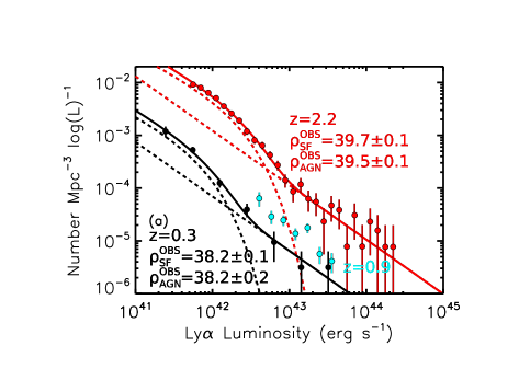
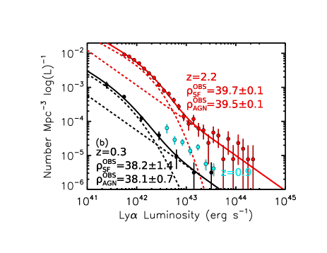
Figure 16.— (a) Evolution of the combined SF and AGN Ly$\alpha$ LFs from $z\sim 0.3$ to $z=2.2$ with best-fit Schechter function $+$ power-law. The black points show our $z\sim 0.3$ LF data. The cyan points show $z\sim 0.9$ LF data from Wold et al. (2014). The red points show the $z=2.2$ LF data from Konno et al. (2016). (b) Same as Figure 16(a), but with the data fit by a Saunders function $+$ power-law. The listed log luminosity densities and corresponding best-fit parameters are summarized in Table 3.

(A color version of this figure is available in the online journal.)

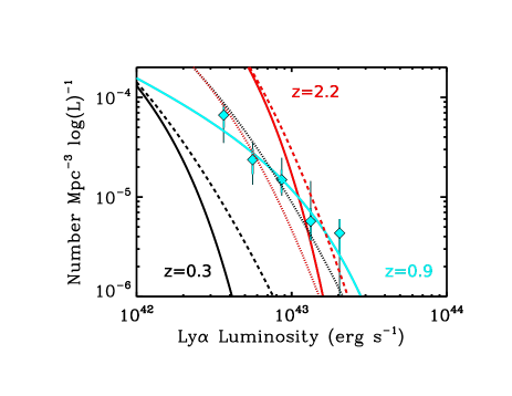
Figure 17.— The $z\sim 0.9$ Ly$\alpha$ SF LF compared to the $z\sim 0.3$ and $z=2.2$ Ly$\alpha$ SF LFs. The cyan data points indicate the $z\sim 0.9$ SF LF with thick Poisson error bars. To assess the effect of any unidentified AGNs, we also show thin error bars that indicate the 1$\sigma$ Poisson error obtained by restricting the $z\sim 0.9$ survey area to regions with deep X-ray data. All SF LAEs within this sub-sample are not identified as AGNs in any way (see Wold et al. 2014 for details) and are known to have X-ray luminosities below $10^{42}$ erg s^-1. The best-fit $z\sim 0.3$, $0.9$, and $2.2$ Schechter functions are indicated by black, cyan, and red solid curves, respectively. The best-fit $z\sim 0.3$ and $2.2$ Saunders functions are indicated by black and red dashed curves, respectively. The $z\sim 0.3$ Saunders function with $L^{\star}$ increased by $0.45$ dex is indicated by the black dotted curve. The $z=2.2$ Saunders function with $\phi^{\star}$ decreased by $0.8$ dex is indicated by the red dotted curve.

(A color version of this figure is available in the online journal.)

For the $z\sim 0.3$ and $2.2$ data, we apply our fitting technique developed in the previous section to obtain self-consistently measured luminosity densities. In this section, we are most interested in a direct comparison of our results to Konno et al. (2016). Thus, for the luminosity density calculations we adopt Konno et al.’s lower integration limit of log $L=41.41$ erg s^-1 that corresponds to $(0.03)L_{Ly\alpha,z=3}^{\star}$ (Ouchi et al., 2008). For the $\rho_{Ly\alpha,AGN}^{obs}$ computations, we set the upper integration limit to the survey’s maximum observed Ly$\alpha$ luminosity. For the $z=0.3$ and $z=2.2$ survey, this corresponds to log $L=$$43.7$ and $44.4$ erg s^-1, respectively .

In Figure 16(a), we simultaneously fit a Schechter function + a fixed slope power-law (listed as fPL in Table 3) to the $z=0.3$ and $z=2.2$ data. It is not clear that our fixed-slope assumption is accurate but given the limited luminosity range over which AGN density dominates over SF galaxies, we adopt this convention. We find that allowing the AGN power-law slope to be a free parameter does not significantly alter our results (see Table 3). Using this simultaneous fitting method, we find a factor of 30 increase in the SF luminosity density from $z\sim 0.3$ to $z=2.2$. Over the same redshift range, Konno et al. (2016) found a more dramatic factor of $\sim 100$ increase in SF luminosity density. The steeper drop found by Konno et al. is caused by their use of the Cowie et al. $z=0.3$ LF. We find a $z=2.2$ log $\rho_{Ly\alpha,SF}^{obs}$ of $39.7\pm 0.1$ erg s^-1Mpc^-3 based on our fit to the data from Konno et al. (2016). Our $z=2.2$ measurement is consistent with the value reported in Konno et al. (log $\rho\sim 39.8$ erg s^-1 Mpc^-3; 2016). Our simultaneous fits favor a lower $L^{\star}$ (by 0.3 dex) and higher $\phi^{\star}$ (by 0.3 dex) at $z=2.2$ than found by Konno et al. (2016, their result labeled ‘Best estimate’). Given the number of assumptions in our fitting method, we do not consider our $L^{\star}$ and $\phi^{\star}$ results to supersede the results of Konno et al. However, if $z=2.2$ AGNs contribute to the overall LAE population in a manner similar to our low-redshift sample, then these proposed offsets may prove to be real.

Comparing our computed $z=2.2$ SF and AGN luminosity densities, we estimate an AGN contribution of $\sim 40\%$ to the total observed Ly$\alpha$ luminosity density with a lower-limit estimate of $\sim 20\%$ . These results are comparable to our previously computed $z\sim 0.3$ AGN contribution estimates of $39\%$ with a lower-limit estimate of $17\%$ (See Section 5). Even if all the low-luminosity AGNs found in our $z=0.3$ sample disappear at $z=2.2$, a significant AGN contribution to the total luminosity density is still expected. For example, integrating the bright-end tail of the AGN LF from $(2.5)L_{{\rm{Ly}\alpha}}^{\star}(z=2.2)=10^{42.8}$ to the observed maximum Ly$\alpha$ luminosity of $10^{44.4}$ erg s^-1, we find that $\rho_{Ly\alpha,AGN}=$39.1 erg s^-1Mpc^-3 which corresponds to an AGN contribution of $\sim 20\%$ to the total observed Ly$\alpha$ luminosity density. These results suggest tentatively that the SF and AGN luminosity densities coevolve from $z=0.3$ to $2.2$ such that star-forming galaxies and AGNs contribute roughly equally to the observed Ly$\alpha$ light.

As in Section 5 and Figure 15, we also consider a Saunders function fit to the data. In Figure16(b), we simultaneously fit a Saunders function + power-law to the $z=0.3$ and $z=2.2$ data. We find that this alteration does not significantly change the measured luminosity densities. Our results are summarized in Table 3. Our main conclusion from these results is that the drop in SF luminosity density from $z=2.2$ to $0.3$ is not as large as some studies have previously claimed (though still very large). Additionally, the contribution of AGNs to the total observed Ly$\alpha$ luminosity density at $z\sim 0.3$ is comparable to the contribution from SF galaxies and this trend appears to continue out to $z=2.2$.

Although the $z\sim 0.9$ data lack sufficient luminosity range to allow us to simultaneously fit the $z\sim 0.9$ SF+AGN LF, in Figure 17 we reproduce the $z\sim 0.9$ SF LF from Wold et al. (2014, cyan curve) to show how the $z\sim 0.3$ and $z=2.2$ SF LFs compare, solid black and red curves, respectively. Taken at face value, the intersection of the best-fit $z\sim 0.9$ Schechter function with the best-fit $z=2.2$ Schechter function implies that SF LAEs more luminous than $\sim 2\times 10^{43}$ erg s^-1 are more common at $z\sim 0.9$ than at $z=2.2$. Over the same redshift range, a similar behavior is not observed in H$\alpha$ LFs (Sobral et al., 2013), and a discordant H$\alpha$ / Ly$\alpha$ LF evolution is not naively expected because to first order Ly$\alpha$ emitting galaxies will be a subset drawn from H$\alpha$ emitting galaxies modulo the escape fraction.

We note that the rate of decline of the Ly$\alpha$ SF LF at high luminosities is difficult to measure due to the increasing AGN contribution, and we suspect that the inferred Ly$\alpha$ LF evolution can be explained by a non-exponential decline in the the bright end of the LF coupled with the attempted Schechter function fit to a very limited and bright $z\sim 0.9$ Ly$\alpha$ luminosity range. As shown in Figure 17, the $z\sim 0.9$ SF LF data-points (cyan diamonds with Poisson error bars) are relatively flat, and they are not well fit by an exponentially declining function. However, we find that our best-fit $z\sim 0.3$ Saunders function with an $L^{\star}$ boost of 0.45 dex (black dotted curve) or our best-fit $z=2.2$ Saunders function with a $\phi^{\star}$ decline by $0.8$ dex (red dotted curve) provide a reasonable fit to the $z\sim 0.9$ SF LF. This implies a $z\sim 0.9$ log $\rho_{Ly\alpha,SF}$ of approximately $38.9$ erg s^-1Mpc^-3 which is $0.5$ dex higher than the SF luminosity density computed from the best-fit Schechter function (see Table 3). We suggest the the previous estimate for $\rho_{Ly\alpha,SF}$ at $z\sim 0.9$ is likely biased low, but we cannot completely rule out alternative explanations such as discordant H$\alpha$ / Ly$\alpha$ LF evolution or undiagnosed AGNs in the $z\sim 0.9$ LAE sample.

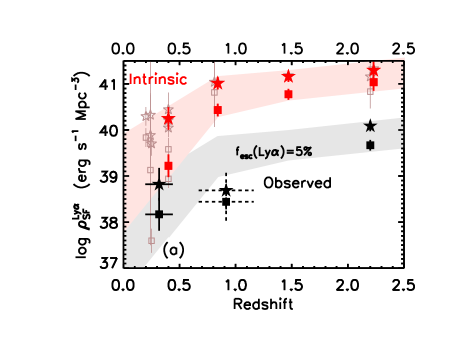
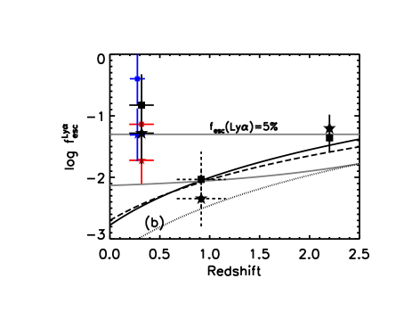
Figure 18.— (a) The evolution of the observed (black symbols) and intrinsic (red symbols) Ly$\alpha$ luminosity densities from $0.3<z<2.2$. Partial luminosity densities are shown with square symbols, while total luminosity densities are shown with star symbols. The red shaded region maps out the intrinsic Ly$\alpha$ luminosity density evolution implied by our fixed $\alpha=-1.6$ fits to Sobral et al.’s H$\alpha$ LFs. The grey region shows this same region offset by -1.3 dex indicating a Ly$\alpha$ escape fraction of $5\%$. The open shaded square and star symbols show partial and total intrinsic Ly$\alpha$ luminosity densities computed from alternative dust-corrected H$\alpha$ LFs (Ly et al. 2007, 2011; Shioya et al. 2008; Lee et al. 2012; Drake et al. 2013; Stroe & Sobral 2015 and total luminosity densities from Sobral et al. 2013). (b) The volumetric Ly$\alpha$ escape fraction computed from the ratio of the observed and intrinsic Ly$\alpha$ luminosity densities. The black star and square symbols show our measured Ly$\alpha$ escape fractions with full and partial integration limits, respectively. The red and blue data points show escape fractions computed from the Ly$\alpha$ studies of Cowie et al. (2010) and Deharveng et al. (2008), respectively. The solid, dashed, and dotted black curves are from Hayes et al. (2011), Blanc et al. (2011), and Konno et al. (2016) , respectively, and show their best fit power law to $f_{esc}({\rm{Ly}}\alpha)$ data. The lower gray curve shows the best fit transition curve from Blanc et al. (2011). The gray horizontal line shows a constant escape fraction of $5\%$. The calculated points and the selected curves have not been corrected for IGM absorption, which should be small for all presented $z<2.2$ data. The $z=0.9$ Ly$\alpha$ luminosity density and escape fraction error bars are dashed because these data points are less secure as discussed in Section 6 and Figure 17.

(A color version of this figure is available in the online journal.)

7. Luminosity Density and Ly$\alpha$ Escape Fraction Evolution

In Figure 18 (a), we show the observed and intrinsic Ly$\alpha$ luminosity density evolution from $z=0.3$ to $2.2$. The observed Ly$\alpha$ luminosity densities are computed from the best-fit Schechter function parameters reported in our Table 3. The intrinsic Ly$\alpha$ luminosity densities are computed from dust-corrected H$\alpha$ LFs from the High-redshift(Z) Emission Line Survey (HiZELS; Sobral et al., 2013). HiZELS is a series of narrow-band surveys that produced self-consistent H$\alpha$ LFs at $z=0.4$, $0.84$, $1.47$, and $2.23$. A constant $A_{{\rm{H}\alpha}}=1$ magnitude of dust extinction correction is applied for all four redshifts, where

$$L_{{\rm{H}\alpha}}=10^{0.4A_{{\rm{H}\alpha}}}L_{{\rm{H}\alpha}}^{{\rm{uncorr}}}.$$ (6)

For consistency with our study, we chose to independently fit the dust-corrected H$\alpha$ LF data (Sobral et al.’s Table 4) with Schechter functions rather than directly using Sobral et al.’s best-fit parameters. Sobral et al. found the faint-end slope of the H$\alpha$ luminosity function to be $\alpha=-1.60\pm 0.08$ with no significant evolution from $z=0.4$ to $2.2$. Thus, we assume a constant $\alpha=-1.6$ for our Schechter functions fits. We find that altering the faint-end to a constant $\alpha=-1.75$, which is consistent with our Ly$\alpha$ LF fits, does not significantly change our results. As prescribed by Sobral et al., we make a 10 to 15$\%$ correction to our H$\alpha$ luminosity densities to account for any AGN contribution (see their Section 4.1). To convert from H$\alpha$ to intrinsic Ly$\alpha$ luminosity, we assume the typical case B recombination ratio of 8.7. In Figure 18 (a), we also show intrinsic Ly$\alpha$ luminosity densities from other dust-corrected H$\alpha$ LFs obtained from the literature. For consistency across both H$\alpha$ and Ly$\alpha$ surveys, we estimate the luminosity density errors by adding in quadrature the reported 1$\sigma$ errors in the best fit Schechter function parameters $L^{\star}$ and $\phi^{\star}$.

As in the previous section, for the Ly$\alpha$ luminosity density calculations we adopt Konno et al.’s lower integration limit of $L=10^{41.41}$ erg s^-1 which corresponds to $10\%$ of our best fit $L_{{\rm{Ly}\alpha}}^{\star}$ at $z=2.2$ (see Table 3). We adopt a consistent H$\alpha$ lower integration limit of $(0.10)L_{{\rm{H}\alpha}}^{\star}(z=2.23)=10^{41.9}$ erg s^-1. Thus, the intrinsic Ly$\alpha$ luminosity densities (square red symbols) are computed with integration limits from $(0.10)L_{{\rm{H}\alpha}}^{\star}(z=2.23)=10^{41.9}$ erg s^-1 to infinity, and the observed Ly$\alpha$ luminosity densities (square black symbols) are computed with integration limits from $(0.10)L_{{\rm{Ly}\alpha}}^{\star}(z=2.2)=10^{41.41}$ erg s^-1 (see Table 3) to infinity.

While our adopted lower integration limits are roughly consistent with the values used by previous studies (e.g., see Hayes et al., 2011; Blanc et al., 2011; Konno et al., 2016), these values are somewhat arbitrary and a source of systematic uncertainty. In particular, we find that the convention of fixing the lower integration limit to a percentage of $L^{\star}$ at high-redshift can contribute to large variations in the computed luminosity densities at low-redshift. Moving from $z=2.2$ to $0$, $L^{\star}$ declines rapidly and if the chosen integration limit approaches $L^{\star}$, then relatively small differences in the best-fit $L^{\star}$ between studies can result in very different luminosity density measures. Integrating down to zero removes this effect but makes our calculation more sensitive to the assumed faint-end slope, but given reasonable $\alpha$ values we do not expect our total luminosity density calculations to be altered by more than a factor of 2. Consistent with this expectation, we find that the variation seen between H$\alpha$ studies in partial luminosity densities (red square symbols) is significantly larger than the variation in total luminosity densities (red star symbols). Given these issues, we consider our total luminosity density measurements to be more reliable when evaluating evolutionary trends, and unless otherwise noted, we use total luminosity densities in the following discussion.

In Figure 18 (a), the red shaded region maps out the intrinsic Ly$\alpha$ luminosity density evolution. The grey region shows this same region offset by -1.3 dex, which corresponds to a Ly$\alpha$ escape fraction of $5\%$. We find that the decline in observed Ly$\alpha$ luminosity density from $z=2.2$ to $z=0.3$ may simply mirror the decline seen in the intrinsic Ly$\alpha$ luminosity density and hence the H$\alpha$ luminosity density. At $z=0.9$, the observed Ly$\alpha$ luminosity density may dip relative to the intrinsic Ly$\alpha$ luminosity density, but this data point is less secure because the luminosity data covers a smaller dynamical range and is limited to the bright end of the LF (see Figure 16).

The volumetric Ly$\alpha$ escape fraction is a measure of the fraction of Ly$\alpha$ photons that escape from the survey volume. It is defined as the ratio of the observed and intrinsic Ly$\alpha$ luminosity densities:

$$f_{esc}^{{\rm{Ly}\alpha}}=\frac{\rho_{Ly\alpha,SF}^{obs}}{\rho_{Ly\alpha,SF}^{int}}=\frac{\rho_{Ly\alpha,SF}^{obs}}{8.7\times\rho_{H\alpha,SF}^{int}}.$$ (7)

Many groups have studied the redshift evolution of this quantity and concluded that the volumetric Ly$\alpha$ escape fraction increases rapidly with redshift until $z=7$ at which point the escape fraction drops, which is typically attributed to the increasing opacity of the IGM and the onset of reionization (Hayes et al., 2011; Blanc et al., 2011; Konno et al., 2016). For this study, we are concerned with the previously claimed rapid decline in $f_{esc}^{{\rm{Ly}\alpha}}$ at low redshifts where the intervening IGM will have a negligible effect. Various explanations for the low-redshift decline have been proposed including increasing dust content and increasing neutral column density of star-forming galaxies. We can now better constrain the escape fraction by including our robust low-redshift constraint and by making a more direct comparison to H$\alpha$ results that are now self-consistently measured out to a redshift of $z=2.23$. Beyond this redshift, H$\alpha$ surveys are not currently available and the intrinsic Ly$\alpha$ luminosities must be estimated from the dust-corrected UV luminosity functions, which require large corrections for extinction and are dependent on the assumed initial mass function, metallicity, and star formation history. We also have the advantage of obtaining all of our H$\alpha$ constraints from a single study (Sobral et al., 2013). This ensures consistency in the employed data reduction and LF incompleteness corrections. We have also assumed the same standard $H_{0}=70$ km s^-1 Mpc^-1, $\Omega_{M}=0.3$, and $\Omega_{\Lambda}=0.7$ cosmology.

In Figure 18 (b), we show the evolution of the volumetric Ly$\alpha$ escape fraction inferred from the intrinsic and observed Ly$\alpha$ luminosity densities presented in Figure 18 (a). Comparing our computed $z=0.3$ and $z=2.2$ Ly$\alpha$ escape fractions, we find results that are consistent with a relatively constant $f_{esc}^{{\rm{Ly}\alpha}}$ with a value of $\sim 10^{-1.3}$ or $\sim 5\%$. The $z=0.9$ data-point may suggest a dip in the escape fraction, but as discussed in Section 6 this data point is less secure. Although our 1$\sigma$ error bars are quite large, we find that the existing low-redshift observational constraints do not provide convincing evidence for rapidly declining $f_{esc}^{{\rm{Ly}\alpha}}$ with decreasing redshift at $0.3<z<2.2$. We emphasize that our results are not inconsistent with an evolving $f_{esc}^{{\rm{Ly}\alpha}}$ at $z>2$. For example, Blanc et al. (2011) found that the overall $0.3<z<7.7$ evolution of $f_{esc}^{{\rm{Ly}\alpha}}$ can be described by a function that levels off at both low-redshift (with $f_{esc}^{{\rm{Ly}\alpha}}(z=0.3)\sim 0.01$) and high-redshift (with $f_{esc}^{{\rm{Ly}\alpha}}(z\sim 6)\sim 0.80$) with a transition between these two extremes at $z\sim 4$. This transitional function was motivated by the observed evolution of dust extinction derived from the UV slope of continuum selected galaxies (Bouwens et al., 2009). Blanc et al.’s best-fit transitional function is shown as a grey curve in Figure 18 (b). While our study favors a higher normalization at low redshifts, the relatively constant $f_{esc}^{{\rm{Ly}\alpha}}$ from $z=0.3$ to $z=2.2$ is consistent with our results.

We find that the difference between our study and previous results (e.g., Hayes et al., 2011; Konno et al., 2016) suggesting a factor of 10 decline in $f_{esc}^{{\rm{Ly}\alpha}}$ from $z=2.2-0.3$ cannot be solely attributed to the numerator, our new $z=0.3$ Ly$\alpha$ LF measurement. Our LF when compared to Cowie et al.’s Ly$\alpha$ LF can only account for a factor of $3$ boost to the $f_{esc}^{{\rm{Ly}\alpha}}(z=0.3)$. To investigate whether the denominator, our $\rho_{Ly\alpha,SF}^{int}(z=0.3)$ measure, is reliable, we compiled measurements from low-redshift dust-corrected H$\alpha$ LFs from the literature (see Figure 18 (a)). Overall, we find that our utilized intrinsic luminosity density is not an outlier when compared to other measurements. If we adopt the highest $\rho_{Ly\alpha,SF}^{int}(z=0.4)=10^{40.48}$erg s^-1Mpc^-3 estimate, which is roughly consistent with the UV derived value used by Konno et al. (2016), we can reduce our $f_{esc}^{{\rm{Ly}\alpha}}(z=0.3)$ measure by an additional factor of 2. We find that other small differences between $f_{esc}^{{\rm{Ly}\alpha}}$ studies are explained by the assumed integration limits, Ly$\alpha$ EW cuts, and best-fit Schechter parameters.

Overall we consider our results that show a relatively constant $f_{esc}^{{\rm{Ly}\alpha}}=0.05$ from $z=0.3-2.2$ to be more reliable because our study has the advantage of a robust $\rho_{Ly\alpha,SF}^{obs}(z=0.3)$ estimate and uniform H$\alpha$ constraints. At the very least, we have shown that the existing low-redshift observational constraints do not provide clear-cut evidence for rapidly evolving $f_{esc}^{{\rm{Ly}\alpha}}$ at $z<2$.

Figure 19.— The observed Ly$\alpha$ luminosity functions (circle symbols) compared to the intrinsic Ly$\alpha$ luminosity functions (shaded diamond and square symbols from Sobral et al. 2013 and Matthee et al. 2017, respectively) with a constant $A_{{\rm{Ly}\alpha}}=3.53$ magnitude of dust extinction applied. Our best-fit H$\alpha$ Schechter functions and our best-fit Ly$\alpha$ Schechter plus power-law functions are shown over the extent of their data-points.

(A color version of this figure is available in the online journal.)

A constant $f_{esc}^{{\rm{Ly}\alpha}}=0.05$ measurement is roughly consistent with expectations given the assumed constant $A_{{\rm{H}\alpha}}=1$ magnitude of dust extinction. Sobral et al. (2013) argue that past H$\alpha$ studies typically find $A_{{\rm{H}\alpha}}=1\pm 0.2$ with no clear redshift evolution. For these reasons, a simple 1 magnitude of H$\alpha$ extinction is corrected for in Sobral et al. and in this study. Assuming a Calzetti et al. (2000) dust law and $R_{V}=4.1$, a magnitude of dust extinction at $\lambda 6563$ implies $A_{{\rm{Ly}\alpha}}=3.53$ mag. In Figure 19, we show the intrinsic Ly$\alpha$ LFs at $z=0.4$, $0.8$, and $2.2$ with a constant 3.53 magnitudes of extinction applied. This is equivalent to multiplying the intrinsic Ly$\alpha$ $L$^⋆ values by a factor of $0.04$ and is consistent with our proposed constant $\sim 5\%$ Ly$\alpha$ escape fraction. Given this very simple assumption the agreement between observed Ly$\alpha$ LFs and intrinsic Ly$\alpha$ LFs with extinction applied is encouraging. Particularly, the agreement is notable for the two narrow-band $z=2.2$ LFs where the bright-end AGN tail becomes dominant at L${}_{{\rm{Ly}\alpha}}\gtrsim 2\times 10^{43}$erg s^-1 in both cases. This scenario implies that within the LAE population the average Ly$\alpha$ photon encounters the same amount of dust opacity as H$\alpha$ photons. This has been previously suggested by studies that examined the relation between the Ly$\alpha$ escape fraction and the dust extinction for samples of LAEs (e.g., Cowie et al. 2011; Blanc et al. 2011). If dust extinction is the main driver of Ly$\alpha$ escape, then this may also help to explain the non-evolution of the Ly$\alpha$ EW scale length since similar to the Ly$\alpha$ escape fraction the EW is also governed by HI scattering and dust absorption, but complicating the interpretation, EWs will also depend on the star formation history and metallicity of the host galaxy. While more complex scenarios cannot be ruled out, we find that the simplest explanation for the lack of evolution observed in the Ly$\alpha$ escape fraction (and perhaps the EW scale length) from $z=0.3$ to $2.2$ is a relatively constant dust extinction over this same redshift range.

8. Summary

Previous studies have suggested that at low redshifts high-EW LAEs become less prevalent and that the amount of Ly$\alpha$ emission able to escape (as measured by $f_{esc}^{{\rm{Ly}\alpha}}$) declines rapidly. A number of explanations for these trends have been suggested including increasing dust content, increasing neutral column density, and/or increasing metallicity of star-forming galaxies at lower redshifts. In this paper we presented the first local sample of LAEs selected based solely on their Ly$\alpha$ emission and showed that the dramatic decline previously suggested in the Ly$\alpha$ EW distribution scale length and volumetric Ly$\alpha$ escape fraction from $z=2.2$ to $0.3$ becomes less convincing when local LAEs are selected in manner similar to high-redshift LAEs. Our results are consistent with these quantities not evolving, despite the intrinsic Ly$\alpha$ luminosity (as probed by $L_{{\rm{H}\alpha}}^{\star}$) plummeting by an order of magnitude from $z=2.2$ to $0.4$ (Sobral et al., 2013). This may imply that the physical conditions that allow strong Ly$\alpha$ emission are present at both low and high redshifts, or that changing conditions conspire make no apparent evolutionary trend. We show that the current Ly$\alpha$ and H$\alpha$ LFs are surprisingly consistent with a simple scenario in which dust extinction is relatively constant and is the main driver of Ly$\alpha$ escape. Finally, our work finds that AGNs contribute significantly to the total Ly$\alpha$ luminosity density, and we find evidence that this holds true out to a redshift of $z=2.2$. We emphasize that larger and more sensitive LAE surveys are needed to further constrain the evolution of the EW distribution scale length and volumetric Ly$\alpha$ escape fraction. The limited facilities currently available in the ultraviolet prevent significant improvement below a redshift of $z\sim 2$. However, the HETDEX survey which will detect close to one million LAEs will resolve whether these quantities evolve from a redshift of $z=2-3.5$.

Table 4Emission-line Sample: CDFS-00

Num	Name	R.A.	Decl.	FUV	NUV	$z^{c}_{\rm{galex}}$	log $L$(Ly$\alpha$)	EWr(Ly$\alpha$)	R.A.(opt)	Decl.(opt)	Offset	$z_{\rm{opt}}$	log $L^{d}_{2-8~{}\rm{keV}}$	Class
		(J2000.0)	(J2000.0)	(AB)	(AB)		(erg s-1)	(Å)	(J2000.0)	(J2000.0)	(arcsec)		(erg s-1)
(1)	(2)	(3)	(4)	(5)	(6)	(7)	(8)	(9)	(10)	(11)	(12)	(13)	(14)	(15)
1	GALEX033102-275130	52.760130	-27.858466	21.97	21.50	0.340	41.95	24$\pm$3	52.760235	-27.858490	0.3	0.335	$\cdots$ string	$\cdots$
2	GALEX033108-2742140	52.785524	-27.704094	23.03	23.44	0.230	41.58	92$\pm$37	52.785574	-27.704395	1.1	$\cdots$ string	$\cdots$ string	$\cdots$
3	GALEX033111-275258	52.797118	-27.882930	21.24	20.62	0.267	41.54	8$\pm$2	52.797794	-27.882475	2.7	0.265	$\cdots$ string	w
4	GALEX033112-274801	52.800331	-27.800321	22.24	21.96	0.260	41.43	18$\pm$6	52.800362	-27.800318	0.1	0.258	$\cdots$ string	$\cdots$
5	GALEX033115-2749530	52.814216	-27.831617	21.20	21.52	0.184	42.17	132$\pm$53	52.814224	-27.831604	0.1	0.182	-999string	$\cdots$
6	GALEX033120-2754490	52.837457	-27.913616	23.62	24.26	0.289	41.97	346$\pm$79	52.836938	-27.913108	2.5	0.290	-999string	$\cdots$
7	GALEX033129-2734490	52.873386	-27.580340	21.47	21.07	0.303	41.48	7$\pm$2	52.872960	-27.580422	1.4	0.297	-999string	$\cdots$
8	GALEX033132-2738030	52.884050	-27.634405	21.95	21.73	0.253			52.884105	-27.634381	0.2	(0.088)	-999string	$\cdots$
9	GALEX033132-2750070	52.885785	-27.835416	21.02	21.01	0.183	41.69	26$\pm$3	52.885924	-27.835377	0.5	0.180	-999string	$\cdots$
10	GALEX033137-2738440	52.906576	-27.645563	23.24	22.80	0.198	41.36	97$\pm$17	52.907163	-27.645389	2.0	0.195	41.4string	$\cdots$
11	GALEX033143-281145	52.930008	-28.196035	22.14	21.91	0.243	41.41	19$\pm$7	52.930058	-28.196028	0.2	0.242	$\cdots$ string	$\cdots$
12	GALEX033145-2810380	52.938978	-28.177395	22.05	23.60	0.218	41.88	85$\pm$9	52.942211	-28.180876	16.2	0.216	$\cdots$ string	$\cdots$
13	GALEX033145-2746150	52.940221	-27.770865	24.83	25.64	0.249	41.27	359$\pm$301	52.939929	-27.770922	1.0	0.247	-999string	a
14	GALEX033147-2808120	52.946718	-28.136678	22.98	23.14	0.286	41.96	129$\pm$54	52.946629	-28.136681	0.3	0.283	$\cdots$ string	$\cdots$
15	GALEX033148-2739460	52.950147	-27.663035	23.44	23.53	0.257	41.60	108$\pm$47	52.950225	-27.662988	0.3	0.259	-999string	$\cdots$
16	GALEX033150-2808110	52.958425	-28.136512	22.74	22.13	0.219	42.24	1110$\pm$381	52.957666	-28.135944	3.2	0.219	$\cdots$ string	n
17	GALEX033150-281120	52.962210	-28.189010	21.01	20.88	0.216	41.74	19$\pm$6	52.962204	-28.189028	0.1	0.213	$\cdots$ string	$\cdots$
18	GALEX033154-281419	52.976513	-28.238641	21.75	21.64	0.282	42.21	67$\pm$23	52.976501	-28.238640	0.0	0.280	$\cdots$ string	$\cdots$
19	GALEX033154-281409	52.978447	-28.235871	21.91	21.27	0.319	41.94	26$\pm$9	52.978458	-28.235889	0.1	0.316	$\cdots$ string	$\cdots$
20	GALEX033155-2812450	52.979571	-28.212720	22.17	22.04	0.329	42.05	42$\pm$14	52.979557	-28.212870	0.5	0.326	$\cdots$ string	$\cdots$
21	GALEX033159-280951	52.999330	-28.164434	21.25	21.15	0.239	41.72	18$\pm$6	52.999458	-28.164722	1.1	0.236	$\cdots$ string	$\cdots$
22	GALEX033200-281057	53.001047	-28.182500	22.46	21.97	0.279	41.81	47$\pm$6	53.002308	-28.182331	4.0	0.278	$\cdots$ string	$\cdots$
23	GALEX033202-2811120	53.010433	-28.186867	23.37	24.22	0.258	41.65	105$\pm$44	53.010105	-28.187319	1.9	0.257	$\cdots$ string	$\cdots$
24	GALEX033204-2804290	53.018110	-28.074785	22.72	22.32	0.282	41.67	42$\pm$15	53.018246	-28.075474	2.5	0.280	42.6string	xn
25	GALEX033211-280911	53.049368	-28.153184	21.09	20.49	0.239	41.44	7$\pm$2	53.049267	-28.152910	1.0	0.237	$\cdots$ string	$\cdots$
26	GALEX033211-280130	53.049749	-28.025048	21.54	21.51	0.218	41.88	52$\pm$18	53.049732	-28.025000	0.2	0.215	-999string	$\cdots$
27	GALEX033213-2804050	53.056197	-28.068263	23.80	22.55	0.298	41.71	133$\pm$25	53.056889	-28.068632	2.6	0.302	-999string	a
28	GALEX033214-2731020	53.059095	-27.517397	22.92	22.53	0.298	41.70	52$\pm$9	53.059971	-27.517139	2.9	0.287	$\cdots$ string	n
29	GALEX033214-281111	53.061569	-28.186519	21.71	21.18	0.263	41.71	21$\pm$2	53.061661	-28.186567	0.3	0.261	$\cdots$ string	n
30	GALEX033216-2813080	53.067724	-28.219051	22.51	22.05	0.278	41.84	55$\pm$7	53.068790	-28.219053	3.4	0.277	$\cdots$ string	$\cdots$
31	GALEX033218-281320	53.078007	-28.222441	21.54	21.16	0.283	42.37	82$\pm$29	53.078033	-28.222441	0.1	0.279	$\cdots$ string	$\cdots$
32	GALEX033219-2741220	53.082533	-27.689716	23.52	23.56	0.229	41.44	108$\pm$19	53.082588	-27.689594	0.5	0.227	41.0string	b
33	GALEX033221-2730440	53.088036	-27.512391	22.75	22.83	0.250	41.62	58$\pm$21	53.088074	-27.512411	0.1	0.248	$\cdots$ string	$\cdots$
34	GALEX033221-2756020	53.088287	-27.934010	22.95	22.75	0.239	41.31	34$\pm$13	53.088452	-27.934212	0.9	0.237	-999string	$\cdots$
35	GALEX033221-2735280	53.091494	-27.591373	23.62	24.11	0.245	41.61	197$\pm$105	53.091785	-27.591337	0.9	0.242	-999string	$\cdots$
36	GALEX033225-2758570	53.107151	-27.982616	23.25	23.55	0.279	41.86	158$\pm$70	53.107237	-27.982728	0.5	0.278	-999string	$\cdots$
37	GALEX033225-2729560	53.107671	-27.499077	23.05	22.82	0.248	41.48	55$\pm$21	53.107868	-27.499100	0.6	0.245	$\cdots$ string	$\cdots$
38	GALEX033232-2757050	53.134436	-27.951597	22.55	22.58	0.233	41.39	29$\pm$10	53.134488	-27.951649	0.2	0.233	-999string	$\cdots$
39	GALEX033234-2747070	53.144657	-27.785525	23.55	23.38	0.248	41.25	51$\pm$21	53.144683	-27.785447	0.3	0.247	39.4string	$\cdots$
40	GALEX033235-2736300	53.148298	-27.608605	22.92	22.53	0.370			53.146029	-27.607698	7.9	(0.251)	-999string	$\cdots$
41	GALEX033236-281038	53.154145	-28.177407	21.32	21.01	0.207	41.75	27$\pm$3	53.155334	-28.177498	3.8	0.204	$\cdots$ string	$\cdots$
42	GALEX033238-2729460	53.159236	-27.496269	23.21	23.47	0.214	41.20	45$\pm$18	53.158962	-27.495813	1.9	0.211	$\cdots$ string	$\cdots$
43	GALEX033241-2736200	53.171766	-27.605734	22.32	22.37	0.260	41.88	65$\pm$23	53.171760	-27.605750	0.1	0.257	-999string	$\cdots$
44	GALEX033241-281125	53.174262	-28.190311	20.03	20.26	0.207	42.29	30$\pm$10	53.174255	-28.190306	0.0	0.204	$\cdots$ string	$\cdots$
45	GALEX033244-2751390	53.184739	-27.860948	22.75	22.26	0.280	41.69	51$\pm$8	53.184493	-27.861438	1.9	0.273	40.8string	n
46	GALEX033244-2745140	53.185187	-27.754043	23.61	24.25	0.263	41.62	145$\pm$66	53.185311	-27.753926	0.6	0.260	-999string	$\cdots$
47	GALEX033246-274714	53.195124	-27.787351	21.97	22.12	0.228	41.85	56$\pm$3	53.195644	-27.787776	2.3	0.226	-999string	$\cdots$

Note. —

Table 4Emission-line Sample: CDFS-00 (Continued)

Num	Name	R.A.	Decl.	FUV	NUV	$z^{c}_{\rm{galex}}$	log $L$(Ly$\alpha$)	EWr(Ly$\alpha$)	R.A.(opt)	Decl.(opt)	Offset	$z_{\rm{opt}}$	log $L^{d}_{2-8~{}\rm{keV}}$	Class
		(J2000.0)	(J2000.0)	(AB)	(AB)		(erg s-1)	(Å)	(J2000.0)	(J2000.0)	(arcsec)		(erg s-1)
(1)	(2)	(3)	(4)	(5)	(6)	(7)	(8)	(9)	(10)	(11)	(12)	(13)	(14)	(15)
48	GALEX033248-2745500	53.201922	-27.764088	22.87	22.96	0.215	41.26	38$\pm$14	53.201833	-27.764037	0.3	0.214	39.6string	$\cdots$
49	GALEX033249-273243	53.208065	-27.545501	21.91	21.81	0.221	41.64	34$\pm$4	53.208122	-27.545031	1.7	0.219	$\cdots$ string	$\cdots$
50	GALEX033251-280305	53.213904	-28.051582	22.30	21.88	0.213	41.77	84$\pm$8	53.214363	-28.051258	1.9	0.214	41.0	a
51	GALEX033253-274834	53.221815	-27.809538	21.57	21.77	0.229	42.16	95$\pm$37	53.221824	-27.809313	0.8	0.226	-999string	$\cdots$
52	GALEX033253-2807040	53.223911	-28.117843	22.15	22.14	0.305	41.82	29$\pm$10	53.223999	-28.117916	0.4	0.297	$\cdots$ string	$\cdots$
53	GALEX033307-274433	53.279518	-27.742550	20.79	20.27	0.220	41.53	10$\pm$1	53.280520	-27.742386	3.2	0.218	40.6string	$\cdots$
54	GALEX033321-273339	53.340413	-27.560853	22.03	21.93	0.278	42.13	76$\pm$27	53.340530	-27.560711	0.6	0.276	-999string	$\cdots$
55	GALEX033333-275645	53.389526	-27.945835	21.80	21.38	0.429	42.12	15$\pm$6	53.389565	-27.946243	1.5	0.422	-999string	$\cdots$
56	GALEX033334-2811270	53.392972	-28.191032	23.41	22.94	0.340	42.06	157$\pm$68	53.393167	-28.191083	0.6	0.338	$\cdots$ string	$\cdots$
57	GALEX033343-2801080	53.431270	-28.019159	23.28	22.09	0.355			53.431339	-28.020054	3.2	(0.656)	$\cdots$ string	$\cdots$
58	GALEX033346-2747360	53.444531	-27.793457	23.36	22.97	0.363	42.43	361$\pm$54	53.445130	-27.793115	2.3	$\cdots$ string	$\cdots$ string	$\cdots$
59	GALEX033351-2735590	53.464008	-27.599818	21.15	20.99	0.184	41.28	10$\pm$4	53.463917	-27.599806	0.3	0.181	$\cdots$ string	$\cdots$
60	GALEX033357-274910	53.489190	-27.819597	21.96	21.65	0.242	41.43	16$\pm$6	53.489895	-27.819418	2.3	0.242	$\cdots$ string	$\cdots$
61	GALEX033359-275759	53.496427	-27.966480	22.16	21.72	0.370	42.21	44$\pm$16	53.496417	-27.966500	0.1	0.358	$\cdots$ string	n
62	GALEX033413-275246	53.555083	-27.879595	21.68	21.66	0.235	41.43	14$\pm$5	53.554714	-27.880039	2.0	0.233	$\cdots$ string	$\cdots$

Note. —

Table 5Emission-line Sample: GROTH-00

Num	Name	R.A.	Decl.	FUV	NUV	$z^{c}_{\rm{galex}}$	log $L$(Ly$\alpha$)	EWr(Ly$\alpha$)	R.A.(opt)	Decl.(opt)	Offset	$z_{\rm{opt}}$	log $L^{d}_{2-10~{}\rm{keV}}$	Class
		(J2000.0)	(J2000.0)	(AB)	(AB)		(erg s-1)	(Å)	(J2000.0)	(J2000.0)	(arcsec)		(erg s-1)
(1)	(2)	(3)	(4)	(5)	(6)	(7)	(8)	(9)	(10)	(11)	(12)	(13)	(14)	(15)
1	GALEX141731+5246100	214.383060	52.769511	22.51	22.54	0.214	41.73	99$\pm$36	214.381970	52.768856	3.3	0.213	$\cdots$	$\cdots$
2	GALEX141745+524618	214.438460	52.771876	22.08	21.84	0.246	41.63	30$\pm$4	214.437670	52.771730	1.8	0.244	-999	$\cdots$
3	GALEX141752+5243160	214.466990	52.721363	23.11	23.19	0.273	41.58	58$\pm$20	214.466800	52.721325	0.4	0.267	-999	$\cdots$
4	GALEX141758+5238110	214.495610	52.636401	23.33	23.21	0.285	41.50	50$\pm$18	214.496290	52.636562	1.6	0.284	-999	$\cdots$
5	GALEX141800+5244010	214.501170	52.733693	22.42	22.44	0.251	41.75	57$\pm$18	214.501820	52.733604	1.5	0.249	-999	$\cdots$
6	GALEX141805+524507	214.521650	52.752176	21.50	21.32	0.245	41.71	20$\pm$6	214.521420	52.751970	0.9	0.244	-999	$\cdots$
7	GALEX141810+5246590	214.541760	52.783332	24.08	22.28	0.360	42.19	542$\pm$195	214.540000	52.784660	6.1	0.356	-999	n
8	GALEX141821+525725	214.588890	52.957118	20.87	20.53	0.384	42.90	50$\pm$14	214.589200	52.957214	0.8	0.379	$\cdots$	ubw
9	GALEX141833+5305400	214.640710	53.094582	22.56	22.77	0.291	41.92	66$\pm$21	214.640470	53.094540	0.5	0.287	$\cdots$	$\cdots$
10	GALEX141845+5256590	214.687990	52.949806	21.93	22.22	0.354	42.48	66$\pm$20	214.687867	52.949653	0.6	0.350	-999	$\cdots$
11	GALEX141851+5224590	214.714340	52.416608	23.82	23.94	0.303	41.65	118$\pm$48	214.714342	52.416469	0.5	0.300	$\cdots$	$\cdots$
12	GALEX141854+530747	214.729040	53.129873	21.72	22.10	0.205	41.73	44$\pm$13	214.728740	53.129887	0.6	0.203	$\cdots$	$\cdots$
13	GALEX141855+525935	214.732990	52.993122	21.92	21.47	0.288	41.79	24$\pm$3	214.732960	52.992176	3.4	0.287	-999	$\cdots$
14	GALEX141859+5223290	214.749790	52.391640	23.03	23.15	0.250	42.02	438$\pm$78	214.749813	52.391408	0.8	0.249	$\cdots$	a
15	GALEX141914+522326	214.812240	52.390660	22.18	21.86	0.256	41.49	21$\pm$7	214.811371	52.390653	1.9	0.252	$\cdots$	$\cdots$
16	GALEX141915+5248250	214.815100	52.807083	22.32	21.88	0.278	41.57	21$\pm$7	214.813220	52.806420	4.7	0.284	-999	$\cdots$
17	GALEX141915+5302460	214.815250	53.046206	23.19	23.33	0.207	41.41	97$\pm$37	214.816610	53.046950	4.0	0.203	$\cdots$	$\cdots$
18	GALEX141920+5302440	214.836310	53.045636	24.81	24.48	0.270	41.56	1100$\pm$917	214.836400	53.046524	3.2	0.271	-999	n
19	GALEX141925+5223330	214.854710	52.392550	23.72	24.14	0.243	41.44	122$\pm$51	214.854700	52.392375	0.6	0.239	$\cdots$	$\cdots$
20	GALEX141934+5256590	214.894880	52.949932	24.13	24.58	0.328	41.81	234$\pm$114	214.895029	52.949811	0.5	0.325	-999	$\cdots$
21	GALEX141937+523024	214.907460	52.506826	21.75	21.18	0.282	41.46	10$\pm$3	214.907440	52.506832	0.0	0.282	$\cdots$	$\cdots$
22	GALEX141938+5230490	214.912120	52.513875	23.33	23.84	0.250	41.67	137$\pm$57	214.912925	52.513550	2.1	0.248	$\cdots$	$\cdots$
23	GALEX141946+5259420	214.943380	52.995262	22.78	21.53	0.275			214.943219	52.995189	0.4	(STAR)string	$\cdots$	$\cdots$
24	GALEX141947+5223040	214.948280	52.384671	22.72	22.47	0.270	41.61	42$\pm$7	214.949570	52.385818	5.0	0.267	$\cdots$	$\cdots$
25	GALEX141951+5242100	214.964510	52.702953	23.80	23.48	0.241			214.964523	52.701321	5.9	(0.549)	43.2	x
26	GALEX141959+5242430	214.998650	52.712043	22.62	22.62	0.241	41.64	59$\pm$21	214.999179	52.712519	2.1	0.240	42.4	xb
27	GALEX142010+5240290	215.042870	52.674995	22.15	21.15	0.319			215.042847	52.674995	0.1	(0.549)	$\cdots$	$\cdots$
28	GALEX142010+5242310	215.045110	52.708868	22.20	22.04	0.239	41.38	18$\pm$3	215.046310	52.707977	4.1	0.239	$\cdots$	n
29	GALEX142011+5229060	215.048720	52.485110	24.30	24.49	0.231	41.29	204$\pm$108	215.048221	52.485156	1.1	0.229	$\cdots$	$\cdots$
30	GALEX142011+5241220	215.049060	52.689652	23.14	23.22	0.224	41.35	131$\pm$55	215.049200	52.689378	1.0	0.221	$\cdots$	$\cdots$
31	GALEX142013+5253570	215.055240	52.899426	23.84	22.89	0.359	42.11	271$\pm$120	215.056592	52.900261	4.2	0.349	-999	$\cdots$
32	GALEX142013+5246520	215.056810	52.781112	22.33	22.17	0.266	41.55	26$\pm$8	215.056690	52.780621	1.8	0.262	-999	$\cdots$
33	GALEX142031+524757	215.132760	52.799350	21.10	20.73	0.253	41.84	17$\pm$2	215.133040	52.799362	0.6	0.253	$\cdots$	$\cdots$
34	GALEX142043+524306	215.180380	52.718352	21.38	21.32	0.251	41.62	14$\pm$4	215.180354	52.718847	1.8	0.247	$\cdots$	$\cdots$
35	GALEX142043+523612	215.181420	52.603344	21.16	20.90	0.341	42.68	68$\pm$21	215.181370	52.603191	0.6	0.337	$\cdots$	ubw
36	GALEX142044+525006	215.186110	52.835135	21.60	21.45	0.255	41.70	20$\pm$6	215.186130	52.835140	0.0	0.251	-999	$\cdots$
37	GALEX142048+5229170	215.203490	52.488241	23.16	22.45	0.239			215.203380	52.488094	0.6	(0.169)	$\cdots$	$\cdots$
38	GALEX142048+5251520	215.203960	52.864454	22.31	21.82	0.213			215.203950	52.864460	0.0	(0.290)	-999	$\cdots$
39	GALEX142051+5243310	215.212510	52.725413	22.70	22.71	0.277	41.55	32$\pm$10	215.212283	52.725239	0.8	0.275	$\cdots$	$\cdots$
40	GALEX142102+5254100	215.259780	52.902805	25.13	23.54	0.188			215.265590	52.903996	13.3	(0.351)	-999	$\cdots$
41	GALEX142121+523805	215.341500	52.634802	21.77	21.63	0.284	42.01	38$\pm$11	215.340940	52.634773	1.2	0.281	$\cdots$	b
42	GALEX142124+523919	215.352620	52.655506	22.07	21.81	0.258	41.60	24$\pm$7	215.352620	52.655499	0.0	0.258	$\cdots$	$\cdots$
43	GALEX142127+5240220	215.363800	52.673039	24.63	23.60	0.281			215.363710	52.672962	0.3	(0.468)	$\cdots$	$\cdots$
44	GALEX142130+5253040	215.375990	52.884719	22.10	22.04	0.195	41.42	33$\pm$10	215.376190	52.884827	0.6	0.193	$\cdots$	$\cdots$
45	GALEX142135+523139	215.399700	52.527553	20.21	20.09	0.250	42.44	39$\pm$12	215.399540	52.527500	0.4	0.249	$\cdots$	ubw
46	GALEX142140+5235120	215.417840	52.586910	22.86	23.00	0.249	41.56	57$\pm$19	215.417750	52.586611	1.1	0.247	$\cdots$	$\cdots$
47	GALEX142151+524950	215.462830	52.830705	21.83	21.64	0.201	41.39	21$\pm$7	215.462970	52.830853	0.6	0.202	$\cdots$	b

Note. —

Table 5Emission-line Sample: GROTH-00 (Continued)

Num	Name	R.A.	Decl.	FUV	NUV	$z^{c}_{\rm{galex}}$	log $L$(Ly$\alpha$)	EWr(Ly$\alpha$)	R.A.(opt)	Decl.(opt)	Offset	$z_{\rm{opt}}$	log $L^{d}_{2-10~{}\rm{keV}}$	Class
		(J2000.0)	(J2000.0)	(AB)	(AB)		(erg s-1)	(Å)	(J2000.0)	(J2000.0)	(arcsec)		(erg s-1)
(1)	(2)	(3)	(4)	(5)	(6)	(7)	(8)	(9)	(10)	(11)	(12)	(13)	(14)	(15)
48	GALEX142157+5245450	215.488030	52.762516	23.34	22.51	0.294			215.488860	52.763329	3.4	(0.381)	$\cdots$	$\cdots$
49	GALEX142206+5236580	215.525010	52.616296	23.33	23.79	0.330	42.11	214$\pm$95	215.525729	52.617000	3.0	0.325	$\cdots$	$\cdots$
50	GALEX142208+525225	215.533960	52.873800	22.49	21.37	0.307	42.05	76$\pm$25	215.533500	52.873810	1.0	0.302	$\cdots$	w
51	GALEX142244+5248050	215.686910	52.801616	23.52	23.28	0.357	42.09	158$\pm$57	215.685780	52.801151	3.0	0.354	$\cdots$	b

Note. —

Table 6Emission-line Sample: NGPDWS-00

Num	Name	R.A.	Decl.	FUV	NUV	$z^{c}_{\rm{galex}}$	log $L$(Ly$\alpha$)	EWr(Ly$\alpha$)	R.A.(opt)	Decl.(opt)	Offset	$z_{\rm{opt}}$	log $L^{d}_{2-7~{}\rm{keV}}$	Class
		(J2000.0)	(J2000.0)	(AB)	(AB)		(erg s-1)	(Å)	(J2000.0)	(J2000.0)	(arcsec)		(erg s-1)
(1)	(2)	(3)	(4)	(5)	(6)	(7)	(8)	(9)	(10)	(11)	(12)	(13)	(14)	(15)
1	GALEX143443+3510520	218.679860	35.181172	22.13	22.20	0.265	41.52	19$\pm$8	218.679520	35.181183	1.0	0.262	-999	$\cdots$
2	GALEX143446+3517030	218.695440	35.284394	21.41	20.92	0.191	41.64	35$\pm$4	218.695370	35.283958	1.6	0.190	41.5	n
3	GALEX143519+3452410	218.829270	34.878325	23.96	23.66	0.234			218.826907	34.877567	7.5	no $z$	-999	$\cdots$
4	GALEX143533+3527410	218.890140	35.461598	24.41	23.58	0.402			218.890710	35.461303	2.0	no $z$	-999	$\cdots$
5	GALEX143544+3500200	218.935920	35.005605	22.43	22.43	0.343	42.07	49$\pm$18	218.935930	35.005558	0.2	0.339	-999	$\cdots$
6	GALEX143554+3519100	218.976530	35.319503	20.80	20.55	0.317			218.977102	35.319122	2.2	(0.552)	42.2	xw
7	GALEX143556+3450060	218.984970	34.835058	22.04	21.64	0.290	42.05	52$\pm$19	218.984820	34.835007	0.5	0.289	-999	$\cdots$
8	GALEX143605+3527290	219.023510	35.458240	21.84	21.21	0.252	41.52	16$\pm$7	219.023280	35.458237	0.7	0.251	-999	$\cdots$
9	GALEX143609+3522420	219.041500	35.378367	21.99	21.85	0.217			219.041391	35.378250	0.5	no $z$	-999	$\cdots$
10	GALEX143613+3448130	219.056080	34.803716	23.15	24.28	0.205	41.78	438$\pm$157	219.055690	34.804249	2.2	0.204	-999	a
11	GALEX143618+3456300	219.077080	34.941691	21.57	21.89	0.271	42.24	62$\pm$23	219.077000	34.941654	0.3	0.269	-999	$\cdots$
12	GALEX143622+345632	219.091790	34.942329	21.27	21.21	0.271	42.01	25$\pm$9	219.092209	34.942055	1.6	0.269	-999	$\cdots$
13	GALEX143624+345938	219.100460	34.993919	21.54	21.50	0.214	41.77	35$\pm$13	219.100418	34.993500	1.5	0.213	-999	$\cdots$
14	GALEX143636+345033	219.152880	34.842770	20.91	20.63	0.283	42.33	36$\pm$12	219.152878	34.842777	0.0	0.280	-999	$\cdots$
15	GALEX143647+3526060	219.197900	35.435101	20.78	20.94	0.180	42.23	84$\pm$31	219.197952	35.435272	0.6	0.178	-999	$\cdots$
16	GALEX143647+3510320	219.198950	35.175702	20.98	20.46	0.253	41.76	13$\pm$2	219.198930	35.175804	0.4	0.251	-999	$\cdots$
17	GALEX143733+352212	219.388110	35.370157	21.11	20.66	0.249	41.84	19$\pm$2	219.388123	35.370167	0.1	0.243	-999	$\cdots$
18	GALEX143738+3522320	219.409870	35.375633	22.39	22.00	0.239	41.84	82$\pm$34	219.410080	35.375557	0.7	0.237	41.4	n
19	GALEX143745+352825	219.437740	35.473771	21.90	21.54	0.396	42.61	71$\pm$25	219.437520	35.473343	1.7	0.394	42.1	xub
20	GALEX143805+345849	219.523550	34.980417	19.50	19.38	0.430	43.04	15$\pm$5	219.523575	34.980476	0.2	0.425	43.1	xubw
21	GALEX143806+3513510	219.528710	35.230987	25.20	23.85	0.334			219.529090	35.231754	3.0	no $z$	-999	$\cdots$
22	GALEX143808+3521110	219.533370	35.353059	25.16	24.97	0.354			219.534508	35.353594	3.9	no $z$	-999	$\cdots$

Note. — Same format as Table 4

Table 7Emission-line Sample: COSMOS-00

Num	Name	R.A.	Decl.	FUV	NUV	$z^{c}_{\rm{galex}}$	log $L$(Ly$\alpha$)	EWr(Ly$\alpha$)	R.A.(opt)	Decl.(opt)	Offset	$z_{\rm{opt}}$	log $L^{d}_{2-10~{}\rm{keV}}$	Class
		(J2000.0)	(J2000.0)	(AB)	(AB)		(erg s-1)	(Å)	(J2000.0)	(J2000.0)	(arcsec)		(erg s-1)
(1)	(2)	(3)	(4)	(5)	(6)	(7)	(8)	(9)	(10)	(11)	(12)	(13)	(14)	(15)
1	GALEX095902+021906	149.761580	2.318473	20.36	20.01	0.350	43.00	69$\pm$19	149.761505	2.318429	0.3	0.345	44.2	xuw
2	GALEX095909+0221540	149.790540	2.365217	24.12	23.02	0.416			149.791031	2.365119	1.8	(0.452)	-999	$\cdots$
3	GALEX095910+0207320	149.793100	2.125737	21.87	21.95	0.357	42.65	103$\pm$30	149.792969	2.125635	0.6	0.353	42.7	xu
4	GALEX095913+0218410	149.804440	2.311585	22.39	22.50	0.245	41.92	82$\pm$28	149.804291	2.311690	0.7	0.250	-999	$\cdots$
5	GALEX095920+0214310	149.837270	2.241971	21.45	21.70	0.307	42.25	36$\pm$10	149.837006	2.241960	1.0	0.303	-999	$\cdots$
6	GALEX095921+0209060	149.840630	2.151739	22.07	22.06	0.360	42.41	66$\pm$11	149.840350	2.151680	1.0	0.355	-999	$\cdots$
7	GALEX095924+0214470	149.852770	2.246435	22.16	21.61	0.348	42.14	39$\pm$12	149.853820	2.245720	4.6	0.345	-999	$\cdots$
8	GALEX095928+0159350	149.868860	1.993090	23.25	22.29	0.255			149.868546	1.992900	1.3	(1.166)	43.6	x
9	GALEX095929+0208490	149.874530	2.147199	22.61	22.76	0.202	41.60	61$\pm$21	149.872147	2.148790	10.3	0.220	-999	$\cdots$
10	GALEX095939+0228380	149.915380	2.477289	22.38	22.70	0.253	41.96	90$\pm$17	149.915110	2.477260	1.0	0.250	-999	$\cdots$
11	GALEX095940+015122	149.917560	1.856112	21.30	21.13	0.251	41.93	25$\pm$7	149.917760	1.855986	0.9	0.251	-999	$\cdots$
12	GALEX095943+0205030	149.930820	2.084299	21.38	21.62	0.189	41.72	34$\pm$10	149.930600	2.083960	1.5	0.186	-999	$\cdots$
13	GALEX095943+0210220	149.932750	2.172934	22.03	21.86	0.263	41.70	25$\pm$8	149.932632	2.173122	0.8	0.262	-999	$\cdots$
14	GALEX095946+0202260	149.942960	2.040575	23.85	24.69	0.394			149.942825	2.040343	1.0	(0.208)	-999	$\cdots$
15	GALEX095950+0225010	149.960410	2.416999	22.83	23.21	0.242	41.80	113$\pm$42	149.960379	2.416972	0.1	0.240	-999	$\cdots$
16	GALEX095955+0231110	149.982740	2.519945	23.97	24.09	0.422			149.983307	2.519970	2.0	no $z$	-999	$\cdots$
17	GALEX095958+0149290	149.995580	1.824732	22.86	22.99	0.221	41.66	102$\pm$37	149.995400	1.824658	0.7	0.219	-999	$\cdots$
18	GALEX100003+0211370	150.012980	2.193794	22.57	22.50	0.238	41.91	126$\pm$48	150.012758	2.193483	1.4	0.238	-999	$\cdots$
19	GALEX100006+0155240	150.026660	1.923501	22.85	22.94	0.265			150.026581	1.923215	1.1	(0.206)	-999	$\cdots$
20	GALEX100006+0222240	150.027990	2.373421	21.28	22.00	0.219	41.62	15$\pm$3	150.028450	2.375111	6.3	0.223	-999	$\cdots$
21	GALEX100010+0154530	150.043040	1.914787	23.94	24.34	0.269	41.69	239$\pm$129	150.042969	1.914580	0.8	0.266	-999	a
22	GALEX100017+0224170	150.074090	2.404956	24.85	25.45	0.288			150.073914	2.405210	1.1	no $z$	-999	$\cdots$
23	GALEX100019+0204380	150.080640	2.077489	23.64	23.30	0.268	41.69	153$\pm$71	150.080279	2.077317	1.4	0.265	-999	$\cdots$
24	GALEX100025+015853	150.105520	1.981567	19.16	19.07	0.379	43.68	80$\pm$21	150.105220	1.981140	1.9	0.372	44.1	xubw
25	GALEX100027+015705	150.115670	1.951455	20.56	20.71	0.268	42.45	38$\pm$10	150.115650	1.951172	1.0	0.265	42.0	$\cdots$
26	GALEX100032+0157210	150.134570	1.955847	22.85	22.79	0.389	42.37	99$\pm$33	150.134384	1.955910	0.7	0.384	-999	$\cdots$
27	GALEX100035+020113	150.148970	2.020404	20.87	20.73	0.269	41.98	16$\pm$4	150.148880	2.020370	0.3	0.266	-999	$\cdots$
28	GALEX100040+0218330	150.169970	2.309275	23.09	24.02	0.266	41.89	151$\pm$58	150.169879	2.308947	1.2	0.262	-999	$\cdots$
29	GALEX100043+020637	150.179780	2.110421	21.76	20.78	0.367	42.61	76$\pm$22	150.179779	2.110381	0.1	0.360	43.3	xub
30	GALEX100047+0204060	150.198650	2.068510	21.56	21.23	0.187	41.90	64$\pm$7	150.198479	2.068497	0.6	0.185	-999	n
31	GALEX100055+0156360	150.232640	1.943342	21.86	23.44	0.220	42.28	238$\pm$40	150.232590	1.942600	2.7	0.219	42.8	xn

Note. —

Table 7Emission-line Sample: COSMOS-00 (Continued)

Num	Name	R.A.	Decl.	FUV	NUV	$z^{c}_{\rm{galex}}$	log $L$(Ly$\alpha$)	EWr(Ly$\alpha$)	R.A.(opt)	Decl.(opt)	Offset	$z_{\rm{opt}}$	log $L^{d}_{2-10~{}\rm{keV}}$	Class
		(J2000.0)	(J2000.0)	(AB)	(AB)		(erg s-1)	(Å)	(J2000.0)	(J2000.0)	(arcsec)		(erg s-1)
(1)	(2)	(3)	(4)	(5)	(6)	(7)	(8)	(9)	(10)	(11)	(12)	(13)	(14)	(15)
32	GALEX100106+0205020	150.277590	2.084125	22.24	21.94	0.284	42.14	83$\pm$25	150.277400	2.084197	0.7	0.283	-999	n
33	GALEX100110+022049	150.294790	2.346956	21.27	21.50	0.250	42.11	41$\pm$11	150.294650	2.347014	0.5	0.248	-999	$\cdots$
34	GALEX100133+0225000	150.388390	2.416912	22.92	22.32	0.349	42.03	64$\pm$20	150.388214	2.417060	0.8	0.350	-999	$\cdots$
35	GALEX100140+0205080	150.418990	2.085591	24.21	23.20	0.377			150.418321	2.085153	2.9	(0.425)	43.4	x
36	GALEX100143+0204370	150.431150	2.077187	24.40	24.01	0.239			150.430496	2.076470	3.5	no $z$	-999	$\cdots$
37	GALEX100150+0224510	150.459720	2.414426	22.42	21.66	0.416			150.459564	2.414530	0.7	(0.267)	-999	$\cdots$
38	GALEX100152+0211580	150.467490	2.199598	21.93	19.93	0.277			150.467380	2.199554	0.4	(STAR)	$\cdots$	$\cdots$

Note. — Same format as Table 4

References

- Adams et al. (2011) Adams, J. J., Blanc, G. A., Hill, G. J., et al. 2011, ApJS, 192, 5
- Adelman-McCarthy & et al. (2009) Adelman-McCarthy, J. K., & et al. 2009, VizieR Online Data Catalog, 2294
- Alexandroff et al. (2015) Alexandroff, R. M., Heckman, T. M., Borthakur, S., Overzier, R., & Leitherer, C. 2015, ApJ, 810, 104
- Assef et al. (2013) Assef, R. J., Stern, D., Kochanek, C. S., et al. 2013, ApJ, 772, 26
- Atek et al. (2009) Atek, H., Kunth, D., Schaerer, D., et al. 2009, A&A, 506, L1
- Baldwin et al. (1981) Baldwin, J. A., Phillips, M. M., & Terlevich, R. 1981, PASP, 93, 5
- Barger et al. (2002) Barger, A. J., Cowie, L. L., Brandt, W. N., et al. 2002, AJ, 124, 1839
- Barger et al. (2012) Barger, A. J., Cowie, L. L., & Wold, I. G. B. 2012, ApJ, 749, 106
- Bertin & Arnouts (1996) Bertin, E., & Arnouts, S. 1996, A&AS, 117, 393
- Blanc et al. (2011) Blanc, G. A., Adams, J. J., Gebhardt, K., et al. 2011, ApJ, 736, 31
- Bouwens et al. (2009) Bouwens, R. J., Illingworth, G. D., Franx, M., et al. 2009, ApJ, 705, 936
- Calzetti et al. (2000) Calzetti, D., Armus, L., Bohlin, R. C., et al. 2000, ApJ, 533, 682
- Cardamone et al. (2010) Cardamone, C. N., van Dokkum, P. G., Urry, C. M., et al. 2010, ApJS, 189, 270
- Cardelli et al. (1989) Cardelli, J. A., Clayton, G. C., & Mathis, J. S. 1989, ApJ, 345, 245
- Ciardullo et al. (2012) Ciardullo, R., Gronwall, C., Wolf, C., et al. 2012, ApJ, 744, 110
- Civano et al. (2016) Civano, F., Marchesi, S., Comastri, A., et al. 2016, ApJ, 819, 62
- Cooper et al. (2012) Cooper, M. C., Yan, R., Dickinson, M., et al. 2012, MNRAS, 425, 2116
- Cowie et al. (2010) Cowie, L. L., Barger, A. J., & Hu, E. M. 2010, ApJ, 711, 928
- Cowie et al. (2011) —. 2011, ApJ, 738, 136
- Cowie et al. (1996) Cowie, L. L., Songaila, A., Hu, E. M., & Cohen, J. G. 1996, AJ, 112, 839
- Deharveng et al. (2008) Deharveng, J.-M., Small, T., Barlow, T. A., et al. 2008, ApJ, 680, 1072
- Drake et al. (2013) Drake, A. B., Simpson, C., Collins, C. A., et al. 2013, MNRAS, 433, 796
- Elvis et al. (2009) Elvis, M., Civano, F., Vignali, C., et al. 2009, ApJS, 184, 158
- Erb et al. (2016) Erb, D. K., Pettini, M., Steidel, C. C., et al. 2016, ArXiv e-prints
- Faber et al. (2003) Faber, S. M., Phillips, A. C., Kibrick, R. I., et al. 2003, in Society of Photo-Optical Instrumentation Engineers (SPIE) Conference Series, Vol. 4841, Society of Photo-Optical Instrumentation Engineers (SPIE) Conference Series, ed. M. Iye & A. F. M. Moorwood, 1657–1669
- Felten (1976) Felten, J. E. 1976, ApJ, 207, 700
- Finkelstein et al. (2009a) Finkelstein, S. L., Cohen, S. H., Malhotra, S., & Rhoads, J. E. 2009a, ApJ, 700, 276
- Finkelstein et al. (2009b) Finkelstein, S. L., Cohen, S. H., Malhotra, S., et al. 2009b, ApJ, 703, L162
- Finkelstein et al. (2011) Finkelstein, S. L., Cohen, S. H., Moustakas, J., et al. 2011, ApJ, 733, 117
- Fitzpatrick (1999) Fitzpatrick, E. L. 1999, PASP, 111, 63
- Flesch (2015) Flesch, E. W. 2015, PASA, 32, e010
- Giacconi et al. (2002) Giacconi, R., Zirm, A., Wang, J., et al. 2002, ApJS, 139, 369
- Gronwall et al. (2007) Gronwall, C., Ciardullo, R., Hickey, T., et al. 2007, ApJ, 667, 79
- Guaita et al. (2010) Guaita, L., Gawiser, E., Padilla, N., et al. 2010, ApJ, 714, 255
- Gunawardhana et al. (2015) Gunawardhana, M. L. P., Hopkins, A. M., Taylor, E. N., et al. 2015, MNRAS, 447, 875
- Hayes et al. (2011) Hayes, M., Schaerer, D., Östlin, G., et al. 2011, ApJ, 730, 8
- Hayes et al. (2013) Hayes, M., Östlin, G., Schaerer, D., et al. 2013, ApJ, 765, L27
- Henry et al. (2015) Henry, A., Scarlata, C., Martin, C. L., & Erb, D. 2015, ApJ, 809, 19
- Hickox et al. (2009) Hickox, R. C., Jones, C., Forman, W. R., et al. 2009, ApJ, 696, 891
- Horne (1986) Horne, K. 1986, PASP, 98, 609
- Hornschemeier et al. (2001) Hornschemeier, A. E., Brandt, W. N., Garmire, G. P., et al. 2001, ApJ, 554, 742
- Hu et al. (2016) Hu, E. M., Cowie, L. L., Songaila, A., et al. 2016, ApJ, 825, L7
- Izotov et al. (2016) Izotov, Y. I., Orlitová, I., Schaerer, D., et al. 2016, Nature, 529, 178
- Jaskot & Oey (2014) Jaskot, A. E., & Oey, M. S. 2014, ApJ, 791, L19
- Kauffmann et al. (2003) Kauffmann, G., Heckman, T. M., Tremonti, C., et al. 2003, MNRAS, 346, 1055
- Kenter et al. (2005) Kenter, A., Murray, S. S., Forman, W. R., et al. 2005, ApJS, 161, 9
- Kewley et al. (2001) Kewley, L. J., Dopita, M. A., Sutherland, R. S., Heisler, C. A., & Trevena, J. 2001, ApJ, 556, 121
- Knobel et al. (2012) Knobel, C., Lilly, S. J., Iovino, A., et al. 2012, ApJ, 753, 121
- Kochanek et al. (2012) Kochanek, C. S., Eisenstein, D. J., Cool, R. J., et al. 2012, ApJS, 200, 8
- Konno et al. (2016) Konno, A., Ouchi, M., Nakajima, K., et al. 2016, ApJ, 823, 20
- Laird et al. (2009) Laird, E. S., Nandra, K., Georgakakis, A., et al. 2009, ApJS, 180, 102
- Lanzuisi et al. (2015) Lanzuisi, G., Perna, M., Delvecchio, I., et al. 2015, A&A, 578, A120
- Le Fèvre et al. (2013) Le Fèvre, O., Cassata, P., Cucciati, O., et al. 2013, A&A, 559, A14
- Lee et al. (2012) Lee, J. C., Ly, C., Spitler, L., et al. 2012, PASP, 124, 782
- Lehmer et al. (2005) Lehmer, B. D., Brandt, W. N., Alexander, D. M., et al. 2005, ApJS, 161, 21
- Lilly et al. (2007) Lilly, S. J., Le Fèvre, O., Renzini, A., et al. 2007, ApJS, 172, 70
- Luo et al. (2008) Luo, B., Bauer, F. E., Brandt, W. N., et al. 2008, ApJS, 179, 19
- Luo et al. (2017) Luo, B., Brandt, W. N., Xue, Y. Q., et al. 2017, ApJS, 228, 2
- Ly et al. (2011) Ly, C., Lee, J. C., Dale, D. A., et al. 2011, ApJ, 726, 109
- Ly et al. (2007) Ly, C., Malkan, M. A., Kashikawa, N., et al. 2007, ApJ, 657, 738
- Mao et al. (2012) Mao, M. Y., Sharp, R., Norris, R. P., et al. 2012, MNRAS, 426, 3334
- Markwardt (2009) Markwardt, C. B. 2009, in Astronomical Society of the Pacific Conference Series, Vol. 411, Astronomical Data Analysis Software and Systems XVIII, ed. D. A. Bohlender, D. Durand, & P. Dowler, 251
- Matthee et al. (2017) Matthee, J., Sobral, D., Best, P., et al. 2017, MNRAS, 471, 629
- Matthee et al. (2015) Matthee, J., Sobral, D., Santos, S., et al. 2015, MNRAS, 451, 400
- Matthews et al. (2013) Matthews, D. J., Newman, J. A., Coil, A. L., Cooper, M. C., & Gwyn, S. D. J. 2013, ApJS, 204, 21
- Morrissey et al. (2007) Morrissey, P., Conrow, T., Barlow, T. A., et al. 2007, ApJS, 173, 682
- Nilsson et al. (2006) Nilsson, K. K., Fynbo, J. P. U., Møller, P., Sommer-Larsen, J., & Ledoux, C. 2006, A&A, 452, L23
- Nilsson & Møller (2011) Nilsson, K. K., & Møller, P. 2011, A&A, 527, L7
- Nilsson et al. (2009) Nilsson, K. K., Tapken, C., Møller, P., et al. 2009, A&A, 498, 13
- Östlin et al. (2014) Östlin, G., Hayes, M., Duval, F., et al. 2014, ApJ, 797, 11
- Ouchi et al. (2008) Ouchi, M., Shimasaku, K., Akiyama, M., et al. 2008, ApJS, 176, 301
- Prescott et al. (2006) Prescott, M. K. M., Impey, C. D., Cool, R. J., & Scoville, N. Z. 2006, ApJ, 644, 100
- Prescott et al. (2015) Prescott, M. K. M., Momcheva, I., Brammer, G. B., Fynbo, J. P. U., & Møller, P. 2015, ApJ, 802, 32
- Rivera-Thorsen et al. (2015) Rivera-Thorsen, T. E., Hayes, M., Östlin, G., et al. 2015, ApJ, 805, 14
- Salim & Lee (2012) Salim, S., & Lee, J. C. 2012, ApJ, 758, 134
- Saunders et al. (1990) Saunders, W., Rowan-Robinson, M., Lawrence, A., et al. 1990, MNRAS, 242, 318
- Scarlata et al. (2009) Scarlata, C., Colbert, J., Teplitz, H. I., et al. 2009, ApJ, 704, L98
- Schaerer (2003) Schaerer, D. 2003, A&A, 397, 527
- Schechter (1976) Schechter, P. 1976, ApJ, 203, 297
- Schirmer et al. (2016) Schirmer, M., Malhotra, S., Levenson, N. A., et al. 2016, MNRAS, 463, 1554
- Schlafly & Finkbeiner (2011) Schlafly, E. F., & Finkbeiner, D. P. 2011, ApJ, 737, 103
- Shapley et al. (2003) Shapley, A. E., Steidel, C. C., Pettini, M., & Adelberger, K. L. 2003, ApJ, 588, 65
- Shioya et al. (2008) Shioya, Y., Taniguchi, Y., Sasaki, S. S., et al. 2008, ApJS, 175, 128
- Sobral et al. (2013) Sobral, D., Smail, I., Best, P. N., et al. 2013, MNRAS, 428, 1128
- Stroe & Sobral (2015) Stroe, A., & Sobral, D. 2015, MNRAS, 453, 242
- Szokoly et al. (2004) Szokoly, G. P., Bergeron, J., Hasinger, G., et al. 2004, ApJS, 155, 271
- Trainor et al. (2016) Trainor, R. F., Strom, A. L., Steidel, C. C., & Rudie, G. C. 2016, ArXiv e-prints
- Trouille & Barger (2010) Trouille, L., & Barger, A. J. 2010, ApJ, 722, 212
- Tumlinson et al. (2003) Tumlinson, J., Shull, J. M., & Venkatesan, A. 2003, ApJ, 584, 608
- Virani et al. (2006) Virani, S. N., Treister, E., Urry, C. M., & Gawiser, E. 2006, AJ, 131, 2373
- Wold et al. (2014) Wold, I. G. B., Barger, A. J., & Cowie, L. L. 2014, ApJ, 783, 119
- York et al. (2000) York, D. G., Adelman, J., Anderson, Jr., J. E., et al. 2000, AJ, 120, 1579
- Zheng et al. (2014) Zheng, Z.-Y., Wang, J.-X., Malhotra, S., et al. 2014, MNRAS, 439, 1101