Abstract

Fractional Gaussian noise (fGn) is a stationary time series model with long memory properties applied in various fields like econometrics, hydrology and climatology. The computational cost in fitting an fGn model of length $n$ using a likelihood-based approach is ${\mathcal{O}}(n^{2})$, exploiting the Toeplitz structure of the covariance matrix. In most realistic cases, we do not observe the fGn process directly but only through indirect Gaussian observations, so the Toeplitz structure is easily lost and the computational cost increases to ${\mathcal{O}}(n^{3})$. This paper presents an approximate fGn model of ${\mathcal{O}}(n)$ computational cost, both with direct or indirect Gaussian observations, with or without conditioning. This is achieved by approximating fGn with a weighted sum of independent first-order autoregressive processes, fitting the parameters of the approximation to match the autocorrelation function of the fGn model. The resulting approximation is stationary despite being Markov and gives a remarkably accurate fit using only four components. The performance of the approximate fGn model is demonstrated in simulations and two real data examples.

Keywords: Autoregressive processes, Gaussian Markov random field, long memory, R-INLA, Toeplitz matrices

1 Introduction

Many natural processes observed in either time or space exhibit long memory dependency structures. One way to characterise long memory is in terms of the autocorrelation function having a slower than exponential decay, as a function of increasing temporal or geographical distance between observational points. In second-order stationary time series, long memory implies that the autocorrelations are not absolutely summable (McLeod and Hipel, 1978). Long memory behaviour has been observed within a vast variety of time series applications, like hydrology (Hurst, 1951; Hosking, 1984), geophysical time series (Mandelbrot and Wallis, 1969), network traffic modelling (Willinger et al., 1996), econometrics (Baillie, 1996; Cont, 2005) and climate data analysis (Franzke, 2012; Rypdal and Rypdal, 2014). For comprehensive introductions to long memory processes and their applications, see for example Doukhan et al. (2003) and Beran et al. (2013).

Fractional Gaussian noise is defined as the increment process of fractional Brownian motion. It is a stationary and parsimoniously parameterised model, with dependency structure characterised by the Hurst exponent $H$, which gives long memory when $1/2<H<1$. The computational cost of likelihood-based inference in fitting an fGn process of length $n$ is ${\mathcal{O}}(n^{2})$, using the Durbin-Levinson or Trench algorithms (McLeod et al., 2007; Golub and Loan, 1996; Durbin, 1960; Levinson, 1947; Trench, 1964). These algorithms make use of the Toeplitz structure of the covariance matrix of fGn and are considered to be sufficiently fast when $n$ is not too large (McLeod et al., 2007). A main problem is that the required Toeplitz structure is fragile to modifications of the Gaussian observational model and computations of conditional distributions. For example, the Toeplitz structure is destroyed if fGn is observed indirectly with Gaussian inhomogeneous noise, or has missing data. Without the Toeplitz structure, the computational cost in fitting fGn increases to ${\mathcal{O}}(n^{3})$, which is far too expensive in many real data applications.

This paper presents an accurate and computationally efficient approximate fGn model of cost ${\mathcal{O}}(n)$, both with direct and indirect Gaussian observations, with or without additional conditioning. This represents a major computational improvement compared with existing approaches, and allows routinely use of fGn models with large $n$, with negligible loss of accuracy. The new approximate model uses a weighted sum of independent first-order autoregressive processes (AR$(1)$). The motivation is that aggregation of short-memory processes plays an important role to explain long memory behaviour in time series (Beran et al., 2010) and an infinite weighted sum of AR(1) processes will give long memory (Granger, 1980). However, the physical intuition about long memory processes suggests that we leverage this relationship much more than the asymptotic result states, see for example Haldrup and Valdés (2017). The new approximate model only needs a weighted sum of a few AR(1) processes to be accurate. We obtain this by fitting the weights and the coefficients of the approximation to mimic the autocorrelation function of the exact fGn model, as a continuous function of $H$.

A key feature of the approximate fGn model is a high degree of conditional independence within the model. Specifically, the approximate model will be represented as a Gaussian Markov random field (GMRF), which computational properties are not destroyed by indirect Gaussian observations nor conditioning (Rue and Held, 2005). The approximate model is also stationary, a desired property which is not common among GMRFs, as they typically have boundary effects. Since the approximate model is a local GMRF, it also fits well within the framework of latent Gaussian models for which approximate Bayesian analysis is obtained with integrated nested Laplace approximations (INLA) (Rue et al., 2009) using the R-package R-INLA (http://www.r-inla.org). A different aspect is that an aggregated model of a few AR$(1)$ components could actually represent a more plausible and interpretable model than fGn in real data applications. Specifically, the approximate model can serve as a tool for automatic source separation in situations where the data at hand represent combined signals.

The plan of this paper is as follows. Section 2 reviews the computational cost in fitting the exact fGn model to direct and indirect Gaussian observations. Section 3 presents the new approximate fGn model and derives the computational cost and memory requirement for evaluating the log-likelihood. The performance of the approximate model is demonstrated by simulations in Section 4, also including a study of its predictive properties. In Section 5, we use the implicit source separation ability in decomposing the historical dataset of annual water level minima for the Nile river (Toussoun, 1925; Beran, 1994). Implementation within the class of latent Gaussian models is demonstrated in analysing a monthly mean surface air temperature series for Central England (Manley, 1953, 1974; Parker et al., 1992). Concluding remarks are given in Section 6.

2 The computational cost of fGn

Let $\boldsymbol{x}=(x_{1},\ldots,x_{n})^{T}$ be a zero-mean fGn process, $\boldsymbol{x}\sim{\mathcal{N}}_{n}(0,\boldsymbol{\Sigma})$. The elements of the covariance matrix, $\Sigma_{ij}=\sigma^{2}\gamma_{\boldsymbol{x}}(k)$, $k=|i-j|$, are defined by the autocorrelation function

$$\gamma_{\boldsymbol{x}}(k)=\frac{1}{2}\Big{(}|k-1|^{2H}-2|k|^{2H}+|k+1|^{2H}\Big{)},\quad k=0,1,\ldots,n-1.$$

This function has a hyperbolic decay $\gamma_{\boldsymbol{x}}(k)\sim H(2H-1)k^{2(H-1)}$ as $k\rightarrow\infty$. The fGn process has long memory when $1/2<H<1$, while it reduces to white noise when $H=1/2$. When $0<H<1/2$, the fGn model has anti-persistent properties, but we do not discuss this case here.

When fGn is observed directly, we estimate $H$ by maximizing the log-likelihood function

$$\log(\pi(\boldsymbol{x}))=-\frac{n}{2}\log(2\pi)+\frac{1}{2}\log|\boldsymbol{Q}|-\frac{1}{2}\boldsymbol{x}^{T}\boldsymbol{Q}\boldsymbol{x},$$

where $\boldsymbol{Q}=\boldsymbol{\Sigma}^{-1}$ is the precision matrix of $\boldsymbol{x}$. Making use of the Toeplitz structure of $\boldsymbol{\Sigma}$, the likelihood is evaluated in $\mathcal{O}(n^{2})$ flops using the Durbin-Levinson algorithm (Golub and Loan, 1996, Algorithm 4.7.2). Also, the precision matrix $\boldsymbol{Q}$ can be calculated in $\mathcal{O}(n^{2})$ flops by the Trench algorithm (Golub and Loan, 1996, Algorithm 4.7.3). In general, the Trench algorithm can be combined with the Durbin-Levinson recursions (Golub and Loan, 1996, Algorithm 5.7.1), to calculate the exact likelihood of general linear Gaussian time series models (McLeod et al., 2007).

A major drawback of relying on these algorithms for Toeplitz matrices is that the Toeplitz structure is easily destroyed if the time series is observed indirectly. Consider a simple regression setting in which an fGn process is observed with independent Gaussian random noise,

$$\boldsymbol{y}=\boldsymbol{x}+\boldsymbol{\epsilon},$$ (1)

where $\boldsymbol{\epsilon}\sim{\mathcal{N}}_{n}(\boldsymbol{0},\boldsymbol{D}^{-1})$ and $\boldsymbol{D}$ is diagonal. The log-density of $\boldsymbol{x}\mid\boldsymbol{y}$ is

$$\log\pi(\boldsymbol{x}\mid\boldsymbol{y})=\frac{1}{2}\log|\boldsymbol{Q}+\boldsymbol{D}|-\frac{1}{2}\boldsymbol{x}^{T}(\boldsymbol{Q}+\boldsymbol{D})\boldsymbol{x}+\boldsymbol{y}^{T}\boldsymbol{D}\boldsymbol{x}+\text{constant}.$$

The conditional mean of $\boldsymbol{x}$ is found by solving $(\boldsymbol{Q}+\boldsymbol{D})\boldsymbol{\mu}_{\boldsymbol{x}\mid\boldsymbol{y}}=\boldsymbol{D}\boldsymbol{y}$ with respect to $\boldsymbol{\mu}_{\boldsymbol{x}\mid\boldsymbol{y}}$, while the marginal variances equal $\mbox{diag}\{(\boldsymbol{Q}+\boldsymbol{D})^{-1}\}$. The Toeplitz structure of $\text{Cov}(\boldsymbol{y})=\boldsymbol{Q}^{-1}+\boldsymbol{D}^{-1}$ is only retained when the noise term has homogeneous variance, i.e. $\boldsymbol{D}^{-1}\propto\boldsymbol{I}$. With non-homogenous observation variance or missing data, the computational cost in fitting (1) would require general algorithms of cost $\mathcal{O}(n^{3})$. This makes analysis of many real data sets infeasible, or at best challenging.

The motivation for expressing the log-likelihood function in terms of the precision matrix $\boldsymbol{Q}$, is to prepare for an approximate GMRF representation of the fGn model. We have already noted that aggregation of an infinite number of short-memory processes can explain long memory behaviour in time series. This implies that $\boldsymbol{Q}$ is (or can be approximated with) a sparse band matrix, but with a larger dimension (still denoted by $n$) for a finite sum. Assume for a moment that such an approximation exists. We can then apply general numerical algorithms for sparse matrices which only depend on the non-zero structure of the matrix. This implies that the numerical cost in dealing with $\boldsymbol{Q}$ or $\boldsymbol{Q}+\boldsymbol{D}$, is the same. Conditioning on subsets of $\boldsymbol{x}$ implies nothing else than working with a submatrix of $\boldsymbol{Q}$ or $\boldsymbol{Q}+\boldsymbol{D}$, and does not add to the computational costs; see (Rue and Held, 2005, Ch. 2) for details. Specifically, we can make use of the Cholesky decomposition, in which the relevant precision matrix $\boldsymbol{Q}+\boldsymbol{D}$ is factorised as $\boldsymbol{Q}+\boldsymbol{D}=\boldsymbol{L}\boldsymbol{L}^{T}$, where $\boldsymbol{L}$ is a lower triangular matrix. The log-likelihood is then evaluated with negligible cost as the log-determinant is $\log|\boldsymbol{Q}+\boldsymbol{D}|=2\sum_{i=1}^{n}L_{ii}$ (Rue, 2001). The conditional mean is found by solving $\boldsymbol{L}\boldsymbol{u}=\boldsymbol{D}\boldsymbol{y}$ and $\boldsymbol{L}^{T}\boldsymbol{\mu}_{\boldsymbol{x}\mid\boldsymbol{y}}=\boldsymbol{u}$. The numerical cost in finding the Cholesky decomposition depends on the non-zero structure of the matrix. For time-series models (or long skinny graphs), the cost is ${\mathcal{O}}(n)$ (Rue and Held, 2005). The explicit construction of such an approximation is discussed next.

3 An approximate fGn model

This section presents an approximate fGn model which is a weighted sum of just a few independent AR$(1)$ processes. We will fit the parameters of the approximation to mimic the autocorrelation structure of fGn up to a given finite lag. The resulting approximate model is a GMRF with a banded precision matrix of fixed bandwidth, which gives a computational cost of ${\mathcal{O}}(n)$.

3.1 Fitting the autocorrelation function

Define $m$ independent AR$(1)$ processes by

$$z_{j,t}=\phi_{j}z_{j,t-1}+\nu_{j,t},\qquad j=1,\ldots,m,\quad t=1,\ldots,n,$$ (2)

where $0<\phi_{j}<1$ denotes the first-lag autocorrelation coefficient of the $j$th AR$(1)$ process. Further, let $\{\nu_{j,t}\}_{j=1}^{m}$ be independent zero-mean Gaussians, with variance $\sigma^{2}_{\nu,j}=(1-\phi_{j}^{2})$. Define the cross-sectional aggregation of the AR$(1)$ processes,

$$\tilde{\boldsymbol{x}}_{m}=\sigma\sum_{j=1}^{m}\sqrt{w_{j}}\boldsymbol{z}^{(j)},$$ (3)

where $\boldsymbol{z}^{(j)}=(z_{j,1},\ldots,z_{j,n})^{T}$ and $\sum_{j=1}^{m}w_{j}=1$. This implies that $\mbox{Var}(\tilde{\boldsymbol{x}}_{m})=\sigma^{2}$. The finite-sample properties of a similar aggregation of AR(1) processes are studied in Haldrup and Valdés (2017), where $w_{j}=1/m$, $\sigma^{2}_{\nu}=1$ and where the coefficients $\phi_{j}$ are Beta distributed. They conclude that “one should be aware that cross-sectional aggregation leading to long memory is an asymptotic feature that applies for the cross-sectional dimension tending to infinity. In finite samples and for moderate cross-sectional dimensions the observed memory of the series can be rather different from the theoretical memory”.

The approximation presented here only needs a small value of the cross-sectional dimension $m$ to be accurate. The key idea to our approach is to fit the weights $\boldsymbol{w}=\{w_{j}\}_{j=1}^{m}$ and the autocorrelation coefficients $\boldsymbol{\phi}=\{\phi_{j}\}_{j=1}^{m}$ in (3) to match the autocorrelation function of fGn, as a function of $H$. The autocorrelation function of (3) follows directly as

$$\gamma_{\tilde{\boldsymbol{x}}_{m}}(k)=\sum_{j=1}^{m}w_{j}\phi_{j}^{|k|},\quad k=0,1,\ldots,n-1.$$

Now, fix a value of $1/2<H<1$. We fit the weights and coefficients $(\boldsymbol{w},\boldsymbol{\phi})_{H}$ by minimizing the weighted squared error

$$(\boldsymbol{w},\boldsymbol{\phi})_{H}=\underset{(\boldsymbol{w},\boldsymbol{\phi})}{\text{argmin}}\sum_{k=1}^{k_{\max}}\frac{1}{k}\big{(}\gamma_{\tilde{\boldsymbol{x}}_{m}}(k)-\gamma_{\boldsymbol{x}}(k)\big{)}^{2},$$ (4)

where $k_{\max}$ represents a user-specified upper limit (we use $k_{\max}=1000$). The squared error is weighted by $1/k$ to ensure a good fit for the autocorrelation function close to lag 0, while less weight is given to tail behaviour as the autocorrelation function is decaying slowly.

By a quite huge calculation done only once, we find $(\boldsymbol{w},\boldsymbol{\phi})_{H}$ for a fine grid of $H$-values. Spline interpolation is used for values of $H$ in between, to represent the weights and coefficients as continuous functions of $H$. The interpolation and fitting are performed using reparameterised weights and coefficients to ensure uniqueness and improved numerical behaviour. These reparameterisations are defined as

$$w_{j}=\frac{e^{v_{j}}}{\sum_{i=1}^{m}e^{v_{i}}}\quad\text{and}\quad\phi_{j}=\frac{1}{1+\sum_{i=1}^{j}e^{-u_{i}}},$$

where $j=1,\ldots,m$ and where $v_{1}=0$. The Hurst exponent is transformed as $H=1/2+1/2\exp(h)/(1+\exp(h))$. This ensures a stable and unconstrained parameter space on $\mathbb{R}^{2m-1}$ for fixed $h$, where $\phi_{1}>\cdots>\phi_{m}$. Note that the error of the fit tends to zero, when $H$ goes to 1 or $1/2$. The resulting coefficients and weights for $m=3$ and $m=4$ are displayed in Figure 1. The fitted weights and coefficients are also available in R using the function INLA::inla.fgn.

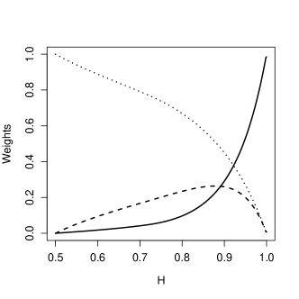
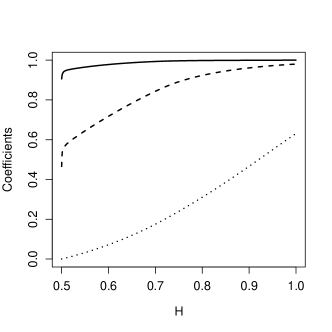
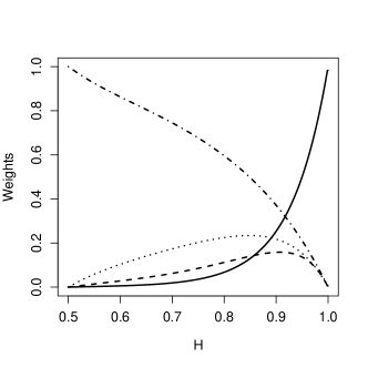
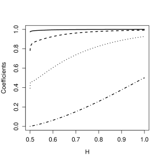
Figure 1: Upper panels: The fitted weights and coefficients $(\boldsymbol{w},\boldsymbol{\phi})_{H}$ in (4) using $m=3$ components in the approximation. Lower panels: Similar using $m=4$.

3.2 A Gaussian Markov random field representation

We will now discuss the precision matrix for the approximate fGn model. We start with one AR$(1)$ process (2) of length $n$, with unit variance and a tridiagonal precision matrix

$$\boldsymbol{R}(\phi_{j})=\frac{1}{1-\phi_{j}^{2}}\begin{pmatrix}1&-\phi_{j}&&&\\ -\phi_{j}&1+\phi_{j}^{2}&-\phi_{j}&&\\ &\ddots&\ddots&\ddots&&\\ &&-\phi_{j}&1+\phi_{j}^{2}&-\phi_{j}\\ &&&-\phi_{j}&1\end{pmatrix}.$$

For the approximate fGn model, we have $m$ such processes and their sum. Hence we need the $(m+1)n\times(m+1)n$ precision matrix of the vector

$$(\tilde{\boldsymbol{x}}_{m}^{T},\boldsymbol{z}^{(1)T},\ldots,\boldsymbol{z}^{(m)T}).$$ (5)

To ensure a non-singular distribution, we will add a small Gaussian noise term to the sum, i.e. we let

$$\tilde{\boldsymbol{x}}_{m}=\sigma\left(\sum_{j=1}^{m}\sqrt{w_{j}}\boldsymbol{z}^{(j)}+\boldsymbol{\epsilon}\right),$$ (6)

where the precision of $\boldsymbol{\epsilon}$ is high, like $\kappa=\exp(15)$. The (upper part of the) precision matrix is found as

$$\begin{pmatrix}\begin{tabular}[]{rrrrr}$\kappa\boldsymbol{I}/\sigma^{2}$&$-\sqrt{w_{1}}\kappa\boldsymbol{I}/\sigma$&$-\sqrt{w_{2}}\kappa\boldsymbol{I}/\sigma$&$\ldots$&$-\sqrt{w_{m}}\kappa\boldsymbol{I}/\sigma$\\ &$\boldsymbol{R}(\phi_{1})+w_{1}\kappa\boldsymbol{I}$&$\sqrt{w_{1}w_{2}}\kappa\boldsymbol{I}$&$\ldots$&$\sqrt{w_{1}w_{m}}\kappa\boldsymbol{I}$\\ &&$\boldsymbol{R}(\phi_{2})+w_{2}\kappa\boldsymbol{I}$&$\ddots$&$\vdots$\\ &&&$\ddots$&$\sqrt{w_{m-1}w_{m}}\kappa\boldsymbol{I}$\\ &&&&$\boldsymbol{R}(\phi_{m})+w_{m}\kappa\boldsymbol{I}$\\ \end{tabular}\end{pmatrix}.$$

The non-zero structure is displayed in Figure 2 (left panel) for $m=3$ and $n=10$. Even though the matrix is sparse, a more optimal structure can be achieved by grouping the $m+1$ variables associated with each of the $n$ time points,

$$\boldsymbol{v}=\left(\tilde{x}_{m1},z^{(1)}_{1},\ldots,z^{(m)}_{1},\;\tilde{x}_{m2},z^{(1)}_{2},\ldots,z^{(m)}_{2},\;\ldots,\;\tilde{x}_{mn},z^{(1)}_{n},z^{(2)}_{n},\ldots,z^{(m)}_{n}\right)^{T}.$$ (7)

The benefit of this reordering is that the corresponding precision matrix $\boldsymbol{Q}_{v}$ is a band matrix, see Figure 2 (middle panel). Doing the Cholesky decomposition, $\boldsymbol{Q}_{v}=\boldsymbol{L}_{v}\boldsymbol{L}_{v}^{T}$, the lower triangular matrix $\boldsymbol{L}_{v}$ will inherit the lower bandwidth of $\boldsymbol{Q}_{v}$ (Rue, 2001; Golub and Loan, 1996, Thm. 4.3.1), see Figure 2 (right panel). This leads to the following key result concerning the computational cost of the approximate model, with a trivial proof.

Theorem 3.1.

The number of flops needed for Cholesky decomposition of $\boldsymbol{Q}_{v}$ is $n(m+1)^{3}$. The memory requirement for the Cholesky triangle is $n(m+1)(m+2)$ reals.

Proof.

$\boldsymbol{Q}_{v}$ is a band matrix with dimension $d=n(m+1)$ and bandwidth $b=m+1$. The computational cost of the Cholesky factorisation, $\boldsymbol{Q}_{v}=\boldsymbol{L}_{v}\boldsymbol{L}_{v}^{T}$ is $db^{2}=n(m+1)^{3}$ and the memory requirement needed is $d(b+1)=n(m+1)(m+2)$ (Golub and Loan, 1996, Section 4.3.5). ∎

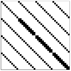
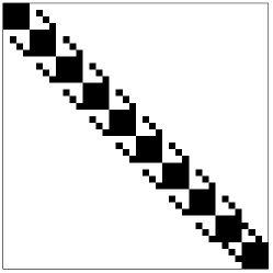
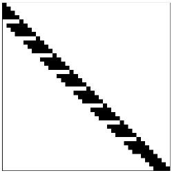
Figure 2: Left panel: The structure of the precision matrix of the vector (5). Middle panel: The structure of the precision matrix of the reordered vector (7). Right panel: The resulting structure of the lower triangular matrix in the Cholesky decomposition. The matrices are illustrated for the case $m=3$ and $n=10$.

The computational cost and memory requirement of the Cholesky decomposition do not change if the approximate fGn model is observed indirectly, like in the regression model (1). Notice that it is also possible to construct an approximation using the cumulative sums of $\sigma\sum_{j=1}^{m}\sqrt{w_{j}}\boldsymbol{z}^{(j)}$ to form a sparse $mn\times mn$ precision matrix, with the same bandwidth. Obviously, this approach gives computational savings but it does not allow for automatic source separation in situations where the fGn can be seen to represent combined signals. This feature of the approximate model is demonstrated in Section 5.1.

3.3 Choosing the number of AR(1) components in the approximation

The choice of $m$ in (6) reflects a trade-off between computational efficiency and approximation error. This implies that $m$ should be as small as possible but still large enough to give a reasonably accurate approximation of the autocorrelation function of fGn. Figure 3 illustrates the autocorrelation function of fGn compared with the approximate model when $m=3$ and $m=4$, using $k_{\max}=1000$ in (4). We only show results for $H=0.9$ as the differences between the curves will be less visible using smaller values of $H$.

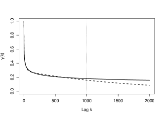
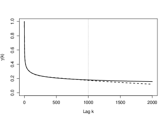
Figure 3: Left panel: The exact autocorrelation function (solid) when $H=0.9$, versus the autocorrelation function of the approximate model (dashed), using $m=3$ and $k_{max}=1000$. Right panel: Similar using $m=4$.

We do notice that $m=4$ gives an almost perfect match of the autocorrelation function up to $k_{\max}$. For larger lags, the autocorrelation function of the approximate fGn model will have an exponential decay, hence we cannot match the hyperbolic decay of the exact fGn. As a consequence, $k_{max}$ can be seen as a trade-off between having a good fit for the first part of the autocorrelation function versus tail behaviour.

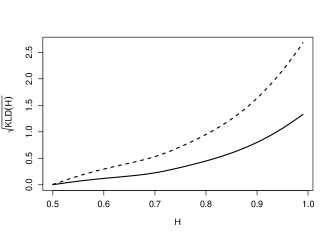
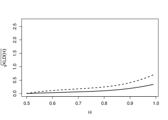
Figure 4: Left panel: The square-root of the Kullback-Leibler divergence as a function of $H$ for time series of length $n=500$ (solid) and $n=2000$ (dashed), using the approximate fGn model with $m=3$. Right panel: Similar using $m=4$.

A different way to illustrate the difference between the approximate and exact fGn models is in terms of the Kullback-Leibler divergence. This is a measure of complexity between probability distributions, which here measures the information lost when the approximate fGn model is used instead of the exact fGn model. Figure 4 displays the square-root of the Kullback-Leibler divergence for $n=500$ and $n=2000$, as a function of $H$. We notice that $m=4$ clearly gives an improvement over $m=3$, in particular for larger values of $H$. The loss in information when $n=2000$ compared to $n=500$ is small, despite the fact that the autocorrelation function is fitted only up to lag $k_{max}=1000$.

4 Simulation results

To evaluate the properties of the approximate fGn model, we now study the loss of accuracy when using the approximate versus the exact fGn model, for estimation and prediction. The results will demonstrate an impressive performance for both the estimation and prediction exercises using the approximate fGn model with $m=4$.

4.1 Maximum likelihood estimation of $H$

We first study the loss of accuracy using the approximate versus the exact fGn model in maximum likelihood estimation of $H$. We fit the approximate model using $m=3$ and $m=4$ to simulated fGn series of length $n=500$, with $N=1000$ replications. The error is evaluated in terms of the root mean squared error (RMSE) and the mean absolute error (MAE) of $\tilde{H}_{i}-\hat{H}_{i}$, where $\tilde{H}_{i}$ and $\hat{H}_{i}$ denote the estimates using the approximate versus the exact fGn, for the $i$th replication.

The results are summarised in Table 1 in which the true Hurst exponent ranges from 0.60 to 0.95. Using $m=3$, the Hurst exponent is underestimated and the error is seen to increase with $H$, at least up to 0.90. The situation really improves for $m=4$, in which the error is small for all values of $H$. The standard deviation estimates found from the empirical Fisher information are more similar than the estimates themselves (results not shown).

	Average MLE of $H$			$\mbox{RMSE}(\tilde{H})$		$\mbox{MAE}(\tilde{H})$
$H$	Exact	$m=3$	$m=4$	$m=3$	$m=4$	$m=3$	$m=4$
0.60	0.5998	0.5998	0.5998	0.0019	0.0007	0.0015	0.0006
0.65	0.6481	0.6478	0.6480	0.0026	0.0008	0.0021	0.0006
0.70	0.7004	0.6997	0.7003	0.0033	0.0008	0.0026	0.0006
0.75	0.7488	0.7472	0.7487	0.0032	0.0007	0.0025	0.0006
0.80	0.7998	0.7974	0.7996	0.0031	0.0006	0.0026	0.0005
0.85	0.8503	0.8471	0.8500	0.0035	0.0004	0.0032	0.0004
0.90	0.8999	0.8965	0.8997	0.0035	0.0003	0.0034	0.0003
0.95	0.9500	0.9475	0.9499	0.0025	0.0002	0.0025	0.0001

Table 1: The average of the maximum likelihood estimates of $H$, the root mean squared error and the absolute mean error using the exact versus the approximate models with $m=3$ and $m=4$. The generated fGn processes are of length $n=500$ with $N=1000$ replications.

Figure 5 displays scatterplots of the maximum likelihood estimates for the approximate model with $m=3$ and $4$, versus the estimates using the exact model, when $H=0.7$, $0.8$ and $0.9$. The inaccuracy for $m=3$ is clearly visible and increases with increasing values of $H$, while $m=4$ shows very good performance. We have noticed that the same general remarks also hold when we increase the length of the series to $n=2000$. The series then contain more information about $H$, and the error due to using $k_{max}=1000$ is negligible. In conclusion, we do get a very low loss of accuracy using the approximate model with $m=4$. This is impressive, especially as it applies for all reasonable values of $H$ in the long memory range.

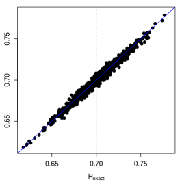
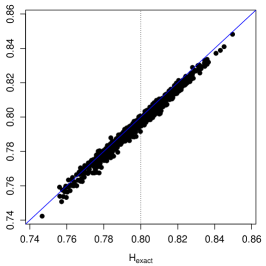
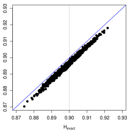
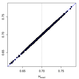
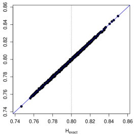
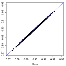
Figure 5: Upper panels: The maximum likelihood estimates of $H$ for $N=1000$ replications using the approximate fGn model with $m=3$ versus the exact fGn (labelled $H_{\mbox{\scriptsize{exact}}}$). The true H-values are $H=0.7$ (left), $H=0.8$ (middle) and $H=0.9$ (right) and the generated series have length $n=500$. Lower panels: Similar using $m=4$.

4.2 Predictive properties

This section investigates the effect of the approximation error when we observe an fGn process of length $n$ with fixed $H$, and then want to predict future time points. The approximate model is implemented with $m=4$. To evaluate the properties of the predictions, we consider the empirical mean of the standardised absolute prediction error,

$$\text{err}_{\mu}(p)=\frac{1}{N}\sum_{i=1}^{N}\frac{|\tilde{\mu}_{p,i}-{\mu}_{p,i}|}{\sigma_{p}},$$ (8)

where $N$ is the number of replications. $\tilde{\mu}_{p,i}$ is the conditional expectation for $p$ time points ahead from the $i$th replication using the approximate fGn model. Correspondingly, ${\mu}_{p,i}$ is the conditional expectation using the exact fGn model while $\sigma_{p}$ is the conditional standard deviation. To measure the error in the conditional standard deviation, we use

$$\text{err}_{\sigma}(p)=\frac{\tilde{\sigma}_{p}}{\sigma_{p}}-1,$$ (9)

which does not depend on the replication.

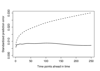
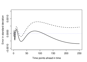
Figure 6: Left panel: The prediction error for the mean (8), predicting up to $250$ points ahead, when $H=0.8$. The observed time series is either of length $n=500$ (solid) or $n=2000$ (dashed). Right panel: The similar error in the conditional standard deviation (9).

The left panel of Figure 6 illustrates the empirical prediction error in (8) for $p=1,\ldots,250$ time-points ahead, following either $n=500$ or $n=2000$ observations. The right panel shows the corresponding error in the prediction standard deviation (9). We only report results for $H=0.8$ as other values of the Hurst exponent give similar results. We notice that the mean prediction error increases slightly when $n=2000$ compared to $n=500$, which is explained by the increased error for lags larger than $k_{\max}=1000$. Otherwise, both errors are relatively small and also quite stable with $p$.

5 Real data applications: Source separation and full Bayesian analysis

This section demonstrates two different aspects of the approximate fGn model in real data applications. First, the approximate model can be used as a tool for source separation of a combined signal, for example representing underlying cycles or variations for different time scales. This will be illustrated in analysing the Nile river dataset (available in R as FGN::NileMin). These data give annual water level minimas for the period 622 - 1284, measured at the Roda Nilometer near Cairo. Second, the approximate model can easily be combined with other model components within the general framework of latent Gaussian models and fitted efficiently using R-INLA. This is demonstrated in analysing the Hadley Centre Central England Temperature series (HadCET), available at http://www.metoffice.gov.uk/hadobs. These data give mean monthly measurements of surface air temperatures for Central England in the period 1659 - 2016. The two datasets are illustrated in Figure 7.

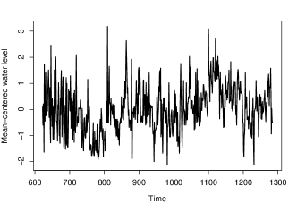
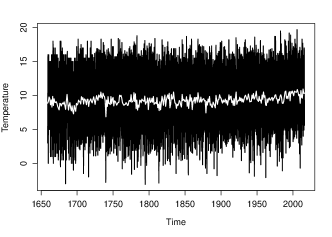
Figure 7: Left panel: Mean-centered annual minimum water level of the Nile river. Right panel: Monthly mean surface air temperatures for Central England, also including the annual mean temperatures in white.

5.1 Signal separation for the Nile river annual minima

The Nile river dataset is a widely studied time series (Beran, 1994; Eltahir, 1996) often used as an example of a real fGn process (Koutsoyiannis, 2002; Benhmehdi et al., 2011). Analysis of this dataset led to the discovery of the Hurst phenomenon (Hurst, 1951). For hydrological time series, this phenomenon has been explained as the tendency of having irregular clusters of wet and dry periods and can be related to characteristics of the fluctuations of the series at different temporal scales (Koutsoyiannis, 2002).

We can easily fit the exact fGn model to this dataset as the process is observed directly and the length of the series is only $n=663$. The maximum likelihood estimate for the Hurst exponent is $\hat{H}=0.831$. Using the approximate fGn model with $m=4$, we get $\hat{H}=0.829$. The resulting four estimated weighted AR(1) components are illustrated in Figure 8. The fitted autocorrelation coefficients for these components equal $\boldsymbol{\phi}=(0.999,0.982,0.847,0.291)$, while the weights are $\boldsymbol{w}=(0.099,0.129,0.232,0.540)$. The estimated standard deviation is $\hat{\sigma}=0.888$.

As illustrated in Figure 1, the first autocorrelation coefficient will always be quite close to 1. This gives a slowly varying trend, which in this case basically represents the mean. The second component also reflects a slowly varying signal, which can be interpreted to represent cycles of the water level fluctuations of about 200 - 250 years. The third component seems to reflect shorter cycles of length 30 - 100 years. These cycles are seen to appear more irregularly and we also notice the tendency of having clusters of years with high and low water levels, respectively. The fourth component, which has the smallest autocorrelation coefficient and the largest weight, can be interpreted as weakly correlated annual noise. These interpretations are in correspondence with the Hurst phenomenon, in which the components reflect signal fluctuations at different temporal scales.

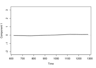
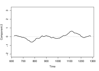
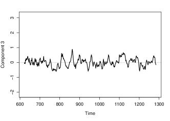
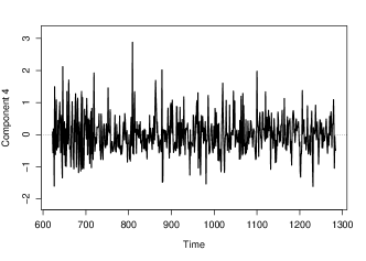
Figure 8: The estimated weighted AR(1) components for mean-centered annual minimum water levels of the Nile river, using the approximate fGn model with $m=4$.

5.2 Full Bayesian analysis of a temperature series

The HadCET series is the longest existing instrumental record of monthly temperatures in the world. The observations started in January 1659 and have been updated monthly. The observed temperatures do have uncertainties (Parker and Horton, 2005), especially in the earliest years, and has been revised several times (Manley, 1953, 1974; Parker et al., 1992). We analyse temperatures up to December 2016, which gives a total of $n=4296$ observations.

In fitting a model to the given temperatures, we assume

$$\text{E}(y_{t})=\beta_{0}+\beta_{1}t+s_{t}+x_{t},\quad t=1,\ldots,4296,$$

where $y_{t}$ is the temperature in month $t$ (measured in degrees Celsius). The given linear predictor includes an intercept $\beta_{0}$, a linear trend $\beta_{1}$, and a seasonal effect $s_{t}$ of periodicity $q=12$ which captures monthly variations. This seasonal effect is modelled as an intrinsic GMRF of rank $n-q+1$, having precision parameter $\tau_{s}$ (Rue and Held, 2005, p. 122) and scaled to have a generalized variance equal to 1 (Sørbye and Rue, 2014). The term $x_{t}$ denotes the approximate fGn model with $m=4$, having precision parameter $\tau_{x}=\sigma^{-2}$.

The parameters $\beta_{0}$ and $\beta_{1}$ are assigned vague Gaussian priors, $\beta_{i}\sim N(0,10^{3})$, while we use penalised complexity priors (PC priors) (Simpson et al., 2017) for all hyperparameters. This implies a type II Gumbel distribution for the precision parameters $\tau_{s}$ and $\tau_{x}$, scaled using the probability statement $P(\tau^{-1/2}>1)=0.01$. The PC prior for $H$ (Sørbye and Rue, 2017) is scaled by assuming the tail probability $P(H>0.9)=0.1$.

Figure 9: The marginal posterior $\pi(H\mid\boldsymbol{y})$, analysing the HadCET data.

Analysis of the given model using an exact fGn term is infeasible in terms of computational cost and memory usage. A MacBook Pro with 16GB of RAM crashes due to memory shortage when analysing exact fGn processes of length $n>2500$. Using the approximate fGn term with $m=4$, the full Bayesian analysis takes about 14 seconds. The inference gives a significantly positive trend with posterior mean $\hat{\beta}_{1}=2.4\cdot 10^{-4}$ with $95\%$ credible interval $(1.2\cdot 10^{-4},3.7\cdot 10^{-4})$. This corresponds to an overall increase in temperature of about $1.05\pm 0.53$ degrees Celsius. The marginal posterior for $H$ is illustrated in Figure 9. The posterior mean is $\hat{H}=0.684$ with $95\%$ credible interval equal to $(0.664,0.704)$.

6 Concluding remarks

In this paper, we obtain a remarkably accurate approximation of fGn using a weighted sum of only four AR$(1)$ components. Our approximate fGn model has a small loss of accuracy for the whole long memory range of $H$. The key idea to obtain this is to ensure that the approximate model captures the most essential part of the autocorrelation structure of the exact fGn model. This is achieved by appropriate weighting, matching the autocorrelation structure up to a specified maximum lag.

By construction, the autocorrelation function of the approximate model has an exponential decay for lags larger than the specified maximum lag. This implies that the approximate model does not satisfy formal definitions of long memory processes. However, this trade-off is needed to make analysis of realistically complex models computationally feasible. The great benefit of the resulting approximation is that it has a GMRF structure. This is crucial, especially as computations can be performed equally efficient in unconditional and conditional scenarios.

An approximate model can never reflect the properties of the exact model perfectly, but neither does a theoretical model in explaining an observed data set. In theory, the fGn model corresponds to an aggregation of an infinite number of AR$(1)$ components which indicates that the model is difficult to interpret in practice. The given decomposition of just a few AR$(1)$ terms might provide a more realistic model. As an example, we have provided a decomposition of the Nile river data, which reflects fluctuations and cycles for different temporal scales. Such a decomposition could also be valuable in analysing climatic time series. For example, long memory in temperature series has been related to an aggregation of a few simple underlying geophysical processes (Fredriksen and Rypdal, 2017).

Implementation of the approximate fGn model in R-INLA provides an easy-to-use tool to analyse models with fGn structure. As demonstrated in the temperature example, we can easily combine the fGn model component with other terms in an additive linear predictor, for example covariates, other random effects or deterministic effects like climate forcing. Also, we do see a potential to incorporate fGn model components in analysis of spatial time series, for example by making use of the methodology in Lindgren et al. (2011).

References

- Baillie (1996) Baillie, R. T. (1996). Long memory processes and fractional integration in econometrics. Journal of Econometrics, 73:5–59.
- Benhmehdi et al. (2011) Benhmehdi, S., Makarava, N., Menhamidouche, N., and Holschneider, M. (2011). Bayesian estimation of the self-similarity exponent of the Nile River fluctuation. Nonlinear Processes in Geophysics, 18:441–446.
- Beran (1994) Beran, J. (1994). Statistics for Long-Memory Processes. Chapman & Hall/CRC, New York, 1st edition.
- Beran et al. (2013) Beran, J., Feng, Y., Ghosh, S., and Kulik, R. (2013). Long-Memory Processes - Probabilistic Properties and Statistical Methods. Springer, Heidelberg.
- Beran et al. (2010) Beran, J., Schützner, M., and Ghosh, S. (2010). From short to long memory: Aggregation and estimation. Computational Statistics and Data Analysis, 54:2432–2442.
- Cont (2005) Cont, R. (2005). Long range dependence in financial markets. In Fractals in Engineering, pages 159–180. Springer, London.
- Doukhan et al. (2003) Doukhan, P., Oppenheim, G., and Taqqu, M. (2003). Theory and Applications of Long-Range Dependence. Birkhauser Boston, c/o Springer-Verlag, New York Inc.
- Durbin (1960) Durbin, J. (1960). The fitting of time-series models. Review of the International Statistical Institute, 28:233–244.
- Eltahir (1996) Eltahir, E. A. B. (1996). El Niño and the natural variability in the flow of the Nile River. Water Resources Research, 32:131–137.
- Franzke (2012) Franzke, C. (2012). Nonlinear trends, long-range dependence, and climate noise properties of surface temperature. Journal of Climate, 25:4172–4182.
- Fredriksen and Rypdal (2017) Fredriksen, H.-B. and Rypdal, M. (2017). Long-range persistence in global surface temperatures explained by linear multibox energy balance models. Journal of Climate, doi.org/10.1175/JCLI-D-16-0877.1.
- Golub and Loan (1996) Golub, G. and Loan, C. V. (1996). Matrix Computations. Johns Hopkins University Press, Baltimore, 3rd edition.
- Granger (1980) Granger, C. W. J. (1980). Long memory relationships and the aggregation of dynamic models. Journal of Econometrics, 14:227–238.
- Haldrup and Valdés (2017) Haldrup, N. and Valdés, J. E. V. (2017). Long memory, fractional integration and cross-sectional aggregation. Journal of Econometrics, 199:1–11.
- Hosking (1984) Hosking, J. R. M. (1984). Modeling persistence in hydrological time series using fractional differencing. Water Resources Research, 20:1898–1908.
- Hurst (1951) Hurst, H. E. (1951). Long-term storage capacities of reservoirs. Transactions of the American Society for Civil Engineers, 116:770–799.
- Koutsoyiannis (2002) Koutsoyiannis, D. (2002). The Hurst phenomenon and fractional Gaussian noise made easy. Hydrological Sciences, 47:573–595.
- Levinson (1947) Levinson, N. (1947). The Wiener (root mean square) error criterion in filter design and prediction. Journal of Mathematics and Physics, 25:261–278.
- Lindgren et al. (2011) Lindgren, F., Rue, H., and Lindström, J. (2011). An explicit link between Gaussian fields and Gaussian Markov random fields: The stochastic partial differential equation approach (with discussion). Journal of the Royal Statistical Society, Series B, 73:423–498.
- Mandelbrot and Wallis (1969) Mandelbrot, B. B. and Wallis, J. R. (1969). Global dependence in geophysical records. Water Resources Research, 5:321–340.
- Manley (1953) Manley, G. (1953). The mean temperature of central England, 1698 to 1952. Quarterly Journal of the Royal Meteorological Society, 79:242–261.
- Manley (1974) Manley, G. (1974). Central England temperatures: Monthly means 1659 to 1973. Quarterly Journal of the Royal Meteorological Society, 100:389–405.
- McLeod and Hipel (1978) McLeod, A. I. and Hipel, K. W. (1978). Preservation of the rescaled adjusted range: 1. A reassessment of the Hurst phenomenon. Water Resources Research, 14:491–508.
- McLeod et al. (2007) McLeod, A. I., Yu, H., and Krougly, Z. L. (2007). Algorithms for linear time series analysis: With R Package. Journal of Statistical Software, 23:1–26.
- Parker and Horton (2005) Parker, D. E. and Horton, E. B. (2005). Uncertainties in the central England temperature series since 1878 and some changes to the maximum and minimum series. International Journal of Climatology, 25:1173–1188.
- Parker et al. (1992) Parker, D. E., Legg, T. P., and Folland, C. K. (1992). A new daily central England temperature series, 1772-1991. International Journal of Climatology, 12:317–342.
- Rue (2001) Rue, H. (2001). Fast sampling of Gaussian Markov random fields. Journal of the Royal Statistical Society, Series B, 63:325–338.
- Rue and Held (2005) Rue, H. and Held, L. (2005). Gaussian Markov Random Fields: Theory and Applications. Chapman & Hall/CRC, London.
- Rue et al. (2009) Rue, H., Martino, S., and Chopin, N. (2009). Approximate Bayesian inference for latent Gaussian models using integrated nested Laplace approximations (with discussion). Journal of the Royal Statistical Society, Series B, 71:319–392.
- Rypdal and Rypdal (2014) Rypdal, M. and Rypdal, K. (2014). Long-memory effects in linear response models of Earth’s temperature and implications for future global warming. Journal of Climate, 27:5240–5258.
- Simpson et al. (2017) Simpson, D., Rue, H., Riebler, A., Martins, T. G., and Sørbye, S. H. (2017). Penalising model component complexity: A principled, practical approach to constructing priors. Statistical Science, 232:1–28.
- Sørbye and Rue (2014) Sørbye, S. H. and Rue, H. (2014). Scaling intrinsic Gaussian Markov random field priors in spatial modelling. Spatial Statistics, 8:39–51.
- Sørbye and Rue (2017) Sørbye, S. H. and Rue, H. (2017). Fractional Gaussian noise: Prior specification and model comparison. Environmetrics, doi:10.1002/env.2457.
- Toussoun (1925) Toussoun, O. (1925). M’emoire sur l’histoire du Nil. In M’emoires a l’Institut d’Egypte, volume 18, pages 366–404.
- Trench (1964) Trench, W. F. (1964). An algorithm for the inversion of finite Toeplitz matrices. Journal of the Society for Industrial and Applied Mathematics, 12:515–522.
- Willinger et al. (1996) Willinger, W., Paxson, V., and Taqqu, M. S. (1996). Self-similarity and heavy tails: Structural modeling of network traffic. In A Practical Guide to Heavy Tails: Statistical Techniques and Applications, pages 27–53. Birkhauser, Boston.