Accelerated sampling by infinite swapping of path integral molecular dynamics with surface hopping

Abstract

To accelerate the thermal equilibrium sampling of multi-level quantum systems, the infinite swapping limit of a recently proposed multi-level ring polymer representation is investigated. In the infinite swapping limit, the ring polymer evolves according to an averaged Hamiltonian with respect to all possible surface index configurations of the ring polymer, thus connects the surface hopping approach to the mean-field path integral molecular dynamics. A multiscale integrator for the infinite swapping limit is also proposed to enable efficient sampling based on the limiting dynamics. Numerical results demonstrate the huge improvement of sampling efficiency of the infinite swapping compared with the direct simulation of path integral molecular dynamics with surface hopping.

I Introduction

This work aims at designing efficient sampling methods of thermal averages of multi-level quantum systems

$$\langle\widehat{A}\rangle=\frac{\operatorname{Tr}_{ne}[e^{-\beta\widehat{H}}\widehat{A}]}{\operatorname{Tr}_{ne}[e^{-\beta\widehat{H}}]},$$ (1)

where $\widehat{H}$ is a multi-level Hamiltonian operator, $\widehat{A}$ is a matrix observable, and $\beta$ is the inverse temperature. The multi-level quantum systems arise when the non-adiabatic effect between different energy surfaces of electronic states cannot be neglected, see e.g., the review articles Makri (1999); Stock and Thoss (2005); Kapral (2006).

The ring polymer representation, originally proposed in Feynman (1972), is an effective way based on path integral to map the quantum thermal average problem to a classical thermal average in an extended phase space. The representation serves as the foundation for various methods, including the path integral Monte Carlo Chandler and Wolynes (1981); Berne and Thirumalai (1986) and path integral molecular dynamics Markland and Manolopoulos (2008); Ceriotti et al. (2010) sampling techniques.

For the multi-level quantum system as in (1), the ring polymer representation can be extended so that each bead in the polymer is associated with a surface index taken into account the multiple levels Schmidt and Tully (2007); Shushkov et al. (2012); Lu and Zhou (2017); Duke and Ananth (2016); Shakib and Huo (2017). Based on the multi-level ring polymer representation, in our previous work Lu and Zhou (2017), a path integral molecular dynamics with surface hopping (PIMD-SH) method is proposed for thermal average calculations, where the discrete electronic state is sampled by a consistent surface hopping algorithm coupled with Hamiltonian dynamics of the position and momentum with Langevin thermostat. Such surface hopping type dynamics for thermal (imaginary time) sampling can be naturally combined with real time surface hopping dynamics Tully (1990); Hammes-Schiffer and Tully (1994); Tully (1998); Kapral (2006); Shenvi et al. (2009); Barbatti (2011); Subotnik and Shenvi (2011); Subotnik et al. (2016); Lu and Zhou (ress, 2016). It is worth emphasizing that, different from Shushkov et al. (2012); Shakib and Huo (2017) where the hopping rate were empirically imposed based on the real time surface hopping dynamics, the hopping process in our previous work Lu and Zhou (2017) satisfies the detailed balance condition and thus the PIMD-SH samples the exact equilibrium distribution of the ring polymer configuration, up to numerical discretization error. Other than the surface hopping approach for which the bead degree of freedom is augmented with a discrete surface index, one could also use the mapping variable approach Meyer and Miller (1979); Stock and Thoss (1997) to extend the conventional ring polymer representation to multi-level systems; see the review article Stock and Thoss (2005) and more recent developments in Ananth and Miller III (2010); Richardson and Thoss (2013); Ananth (2013); Menzeleev et al. (2014); Cotton and Miller (2015); Hele and Ananth (2016); Liu (2016) Let us also mention the related sampling approaches for reduced density matrix for open quantum systems of a system coupled to harmonic bath Moix et al. (2012); Montoya-Castillo and Reichman (2017).

While the PIMD-SH method has been validated through numerical examples in Lu and Zhou (2017), it is observed that sampling off-diagonal elements of the observable, associated with the coupling between different energy surfaces, is more challenging. This is due to the fact that in the ring polymer representation, only consecutive beads living on different energy surfaces (referred to as a kink) can make major contribution to the average; while these kinks are rare to form in the PIMD-SH dynamics since such configuration has higher energy compared to configurations without kinks.

As noted in Lu and Zhou (2017), it is possible to increase the hopping frequency $\eta$ so that the ring polymer develops kinks on a faster time scale, in fact, it can be proved that the sampling efficiency increases as the hopping intensity parameter increases. However, at the same time, a faster hopping dynamics increases the stiffness of the dynamics and hence makes the numerical integration more challenging.

To overcome this difficulty, in this work, we will investigate the infinite swapping limit of the ring polymer representation for multi-level quantum systems. When the hopping frequency $\eta\gg 1$, there are two distinct time scales in the trajectory evolution under PIMD-SH: the fast scale is characterized by the typical time length of changes in the surface index (hopping), and the slow scale corresponds to the Langevin dynamics. Thus, the infinite swapping limit can be viewed as the homogenization limit of a multiscale dynamical systems Pavliotis and Stuart (2008); E (2011). As we will show, as the hopping intensity parameter $\eta$ goes to infinity, the averaging leads to an explicit limiting dynamics of only the slow variables, the position and momentum of beads in the ring polymer, while the fast variables are effectively in local equilibrium and can be integrated out. We show that the PIMD-SH converges to the mean-field ring polymer representation Prezhdo and Rossky (1997); Duke and Ananth (2016) in the infinite swappling limit. This connection facilitates the design of numerical integrators for sampling the ring polymer configuration for thermal averages.

To simulate the infinite swapping dynamics, we borrow the idea from heterogeneous multiscale methods (HMM) E and Engquist (2003); Vanden-Eijnden (2003); E et al. (2007); E (2011) for multiscale dynamics systems (see also earlier works of multiple time-stepping methods with similar ideas Gear and Wells (1984); Tuckerman et al. (1990); Tuckerman and Berne (1991a, b, c)), in particular, the recently developed multiscale integrator for replica exchange method when the swapping frequency is high Yu et al. (2016); Lu and Vanden-Eijnden (2017) by one of us. Our proposed multiscale integrator effectively samples the ring polymer representation for $\eta\gg 1$, while avoiding the enumeration of all possible surface index configurations at every time step. Following the spirit of Yu et al. (2016), the multiscale integrator consists of a macrosolver for the Langevin dynamics and a microsolver for the continuous-time Markov jump process of the surface index, with the two linked by an estimator passing information from micro- to macro-solvers. The details are presented in §III.2. The multiscale integrator efficiently samples the thermal average based on the infinite swapping dynamics, especially when the potential landscape is complicated or the temperature is low, so that it is necessary to use more beads in the ring polymer representation.

The paper is outlined as follows. In Section II, we briefly review the ring polymer representation for the thermal averages for multi-level quantum systems and its direct simulation method. The derivation of the infinite swapping limit is then presented in detail, with discussions on its efficiency compared to the PIMD-SH method. We discuss the numerical algorithms in simulating the PIMD-SH and its infinite swapping limit in Section III, highlighting a multiscale integrator proposed in this work. Numerical tests are presented in Section IV to validate the proposed algorithms.

II Theory

II.1 Thermal equilibrium average of two-level quantum systems and its ring polymer representation

Consider the thermal equilibrium average of observables as in (1) for an operator $\widehat{A}$ and a two level Hamiltonian $\widehat{H}$, where $\beta=(k_{B}T)^{-1}$ with $k_{B}$ the Boltzmann constant and $T$ the absolute temperature. Here, the Hamiltonian is given by

$$\widehat{H}=\widehat{T}+\widehat{V}=\frac{1}{2M}\begin{pmatrix}\widehat{p}^{2}&\\ &\widehat{p}^{2}\end{pmatrix}+\begin{pmatrix}V_{00}(\widehat{q})&V_{01}(\widehat{q})\\ V_{10}(\widehat{q})&V_{11}(\widehat{q})\end{pmatrix},$$

where $\widehat{q}$ and $\widehat{p}$ are the nuclear position and momentum operators, $V(q)$ is a Hermitian matrix for all $q\in{\mathbb{R}}^{d}$, and $M$ is the mass of nuclei (for simplicity we assume all nuclei have the same mass). The Hilbert space of the system is thus $L^{2}({\mathbb{R}}^{d})\otimes{\mathbb{C}}^{2}$, where $d$ is the spatial dimension of the nuclei position degree of freedom, and thus $\operatorname{Tr}_{ne}$ in (1) denotes trace with respect to both the nuclear and electronic degrees of freedom, namely, $\operatorname{Tr}_{ne}=\operatorname{Tr}_{n}\operatorname{Tr}_{e}=\operatorname{Tr}_{L^{2}({\mathbb{R}}^{d})}\operatorname{Tr}_{{\mathbb{C}}^{2}}$. The denominator in (1) is the partition function given by $\mathcal{Z}=\operatorname{Tr}_{ne}[e^{-\beta\widehat{H}}]$. For simplicity, we will assume that the off-diagonal potential functions $V_{01}=V_{10}$ are real valued and do not change sign. We also assume that the observable $\widehat{A}$ only depends on $q$, but it may have off-diagonal elements. As we shall illustrate in Section II.2, sampling off-diagonal elements of $\widehat{A}$ is more challenging with the ring polymer representation, which will be the focus of our current paper.

In this following, we briefly summarize the ring polymer representation of (1) proposed in our previous work Lu and Zhou (2017), and more details can be found in Appendix A. With the ring polymer representation, the thermal average (1) can be approximated by an average with respect to the classical Gibbs distribution for ring polymers on the extended phase space with Hamiltonian $H_{N}$:

$$\langle\widehat{A}\rangle\approx\frac{1}{(2\pi)^{dN}}\int_{{\mathbb{R}}^{2dN}}\,\mathrm{d}\boldsymbol{q}\,\mathrm{d}\boldsymbol{p}\sum_{\boldsymbol{\ell}\in\{0,1\}^{N}}\pi(\widetilde{\boldsymbol{z}})W_{N}[A](\widetilde{\boldsymbol{z}}),$$ (2)

with distribution

$$\pi(\widetilde{\boldsymbol{z}})=\frac{1}{\mathcal{Z}_{N}}\exp(-\beta_{N}H_{N}(\widetilde{\boldsymbol{z}})),$$ (3)

To simplify the notation, we have denoted by $\widetilde{\boldsymbol{z}}=(\boldsymbol{z},\boldsymbol{\ell})\in{\mathbb{R}}^{dN}\times{\mathbb{R}}^{dN}\times\{0,1\}^{N}$ a state vector on the extended phase space, where $\boldsymbol{z}=(\boldsymbol{q},\boldsymbol{p})$ are the position and momentum variables. To be more specific, $\boldsymbol{q}=(q_{1},\cdots,q_{N})$ and $\boldsymbol{p}=(p_{1},\cdots,p_{N})$ are the position and momentum of each bead, and $\boldsymbol{\ell}=(\ell_{1},\cdots,\ell_{N})$ indicates the surface index of the bead (thus each bead in the ring polymer lives on two copies of the classical phase space ${\mathbb{R}}^{2d}$, see Figure 1 for a schematic plot). In particular, when $\ell_{k}\neq\ell_{k+1}$, two consecutive $k$-th and $(k+1)$-th beads in the ring polymer stay on different energy surfaces; this will be referred to as a kink in the ring polymer. Notice that in (3), $\mathcal{Z}_{N}$ normalizes the distribution in the sense that

$$\frac{1}{(2\pi)^{dN}}\int_{{\mathbb{R}}^{2dN}}\,\mathrm{d}\boldsymbol{q}\,\mathrm{d}\boldsymbol{p}\sum_{\boldsymbol{\ell}\in\{0,1\}^{N}}\pi(\widetilde{\boldsymbol{z}})=1.$$

The expressions for $W_{N}[A]$ and $H_{N}$ can be found in Appendix A, and the readers may also refer to Lu and Zhou (2017) for detailed derivations.

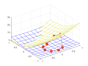
Figure 1: Schematic plot of a ring polymer on the extended phase space with two diabatic energy surfaces.

II.2 Molecular dynamics sampling of the ring polymer representation

With the ring polymer representation, it is then natural to construct a sampling algorithm for $\pi$ as in(3) and thus to approximate the ensemble average in the ring polymer representation given by (2). In our previous work Lu and Zhou (2017), a path-integral molecular dynamics with surface hopping (PIMD-SH) method was proposed, which we will review here. We also discuss its difficulty for sampling off-diagonal elements of $\widehat{A}$, which motivates the development of improved algorithms in the current work.

The PIMD-SH method samples the ring polymer representation by simulating a long trajectory $\widetilde{\boldsymbol{z}}(t)$ that is ergodic with respect to the equilibrium distribution $\pi$, and thus the ensemble average on the right hand side of (2) is approximated by a time average

$$\langle\widehat{A}\rangle\approx\lim_{T\rightarrow\infty}\frac{1}{T}\int_{0}^{T}W_{N}[A](\widetilde{\boldsymbol{z}}(t))\,\mathrm{d}t.$$ (4)

The dynamics of $\widetilde{\boldsymbol{z}}(t)$ is constructed as follows. The position and momentum part of the trajectory $\boldsymbol{z}(t)=(\boldsymbol{q}(t),\boldsymbol{p}(t))$ evolves according to a Langevin dynamics with Hamiltonian $H_{N}(\boldsymbol{q}(t),\boldsymbol{p}(t),\boldsymbol{\ell}(t))$ given the surface index $\boldsymbol{\ell}(t)$, i.e., a Langevin thermostat is used. More specifically, we have

$$\left\{\begin{array}[]{l l}\,\mathrm{d}{\boldsymbol{q}}&=\nabla_{\boldsymbol{p}}H_{N}(\boldsymbol{q}(t),\boldsymbol{p}(t),\boldsymbol{\ell}(t))\,\mathrm{d}t,\vspace{0.2cm}\\ \,\mathrm{d}{\boldsymbol{p}}&=-\nabla_{\boldsymbol{q}}H_{N}(\boldsymbol{q}(t),\boldsymbol{p}(t),\boldsymbol{\ell}(t))\,\mathrm{d}t\vspace{0.1cm}\\ &\qquad\qquad-\gamma\boldsymbol{p}\,\mathrm{d}t+\sqrt{2\gamma\beta^{-1}_{N}M}\,\mathrm{d}\boldsymbol{B}.\end{array}\right.$$ (5)

Here $\boldsymbol{B}=\boldsymbol{B}(t)$ is a vector of $dN$ independent Brownian motions (thus the derivative of each component is an independent white noise), and $\gamma\in\mathbb{R}_{+}$ denotes the friction constant, as usual in Langevin dynamics. By direct calculation, we notice that the evolution of the position just follows as usual

$$\,\mathrm{d}{\boldsymbol{q}}=\frac{1}{M}\boldsymbol{p}\,\mathrm{d}t.$$

The forcing term of the $\boldsymbol{p}$-equation, given by $-\nabla_{\boldsymbol{q}}H_{N}(\boldsymbol{q}(t),\boldsymbol{p}(t),\boldsymbol{\ell}(t))$, is in general $\boldsymbol{\ell}(t)$-dependent, as the potential energy depends on the level index. The dissipation and fluctuation terms are clearly independent of $\boldsymbol{\ell}(t)$.

The evolution of $\boldsymbol{\ell}(t)$ follows a surface hopping type dynamics in the spirit of the fewest switches surface hopping Tully (1990); Lu and Zhou (ress, 2016), which is a Markov jump process with infinitesimal transition rate over the time period $(t,t+\delta t)$ for $\delta t\ll 1$ given by

$$\mathbb{P}\bigl{(}\boldsymbol{\ell}(t+\delta t)=\boldsymbol{\ell}^{\prime}\mid\boldsymbol{\ell}(t)=\boldsymbol{\ell}\,,\boldsymbol{z}(t)=\boldsymbol{z}\bigr{)}\\ =\delta_{\boldsymbol{\ell}^{\prime},\boldsymbol{\ell}}+\eta\lambda_{\boldsymbol{\ell}^{\prime},\boldsymbol{\ell}}(\boldsymbol{z})\delta t+o(\delta t).$$ (6)

Here, $\eta>0$ is an overall scaling parameter for hopping intensity, and the coefficients $\lambda_{\boldsymbol{\ell}^{\prime},\boldsymbol{\ell}}$ are given by

$$\lambda_{\boldsymbol{\ell}^{\prime},\boldsymbol{\ell}}(\boldsymbol{z})=\begin{cases}\displaystyle-\sum_{\widetilde{\boldsymbol{\ell}}\in S_{\boldsymbol{\ell}}}p_{\widetilde{\boldsymbol{\ell}},\boldsymbol{\ell}}(\boldsymbol{z}),&\boldsymbol{\ell}^{\prime}=\boldsymbol{\ell},\\ p_{\boldsymbol{\ell}^{\prime},\boldsymbol{\ell}}(\boldsymbol{z}),&\boldsymbol{\ell}^{\prime}\in S_{\boldsymbol{\ell}},\\ 0,&\text{otherwise}.\end{cases}$$ (7)

In the expression above, $S_{\boldsymbol{\ell}}$ denotes the accessible surface index set from $\boldsymbol{\ell}$ by one “jump”, which is chosen to be $S_{\boldsymbol{\ell}}=\{\boldsymbol{\ell}^{\prime}\mid\lVert\boldsymbol{\ell}^{\prime}-\boldsymbol{\ell}\rVert_{1}=1\;\mbox{or}\;\boldsymbol{\ell}^{\prime}=\boldsymbol{1}-\boldsymbol{\ell}\}$, where $\boldsymbol{1}$ is the vector with all entries $1$. Hence $\boldsymbol{\ell^{\prime}}=\boldsymbol{1}-\boldsymbol{\ell}$ indicates that the surface index of each bead is flipped; and $\lVert\boldsymbol{\ell^{\prime}}-\boldsymbol{\ell}\rVert_{1}=\sum_{k}\lvert\ell^{\prime}_{k}-\ell_{k}\rvert=1$ indicates that one and only one bead jumps to the opposite energy surface. Here in the rate expression, $p_{\boldsymbol{\ell}^{\prime},\boldsymbol{\ell}}(\boldsymbol{z})$ is defined as

$$p_{\boldsymbol{\ell}^{\prime},\boldsymbol{\ell}}(\boldsymbol{z})=\exp\left(\frac{\beta_{N}}{2}\bigl{(}H_{N}(\boldsymbol{z},\boldsymbol{\ell})-H_{N}(\boldsymbol{z},\boldsymbol{\ell}^{\prime})\bigr{)}\right),$$ (8)

which is chosen so that the detailed balance relation is satisfied

$$p_{\boldsymbol{\ell}^{\prime},\boldsymbol{\ell}}(\boldsymbol{z})e^{-\beta_{N}H_{N}(\boldsymbol{z},\boldsymbol{\ell})}=e^{-\frac{\beta_{N}}{2}\bigl{(}H_{N}(\boldsymbol{z},\boldsymbol{\ell})+H_{N}(\boldsymbol{z},\boldsymbol{\ell}^{\prime})\bigr{)}}\\ =p_{\boldsymbol{\ell},\boldsymbol{\ell}^{\prime}}(\boldsymbol{z})e^{-\beta_{N}H_{N}(\boldsymbol{z},\boldsymbol{\ell}^{\prime})}.$$ (9)

This guarantees that the distribution $\pi$ is preserved under the dynamics of the jumping process. Moreover, it has been proved in Lu and Zhou (2017) that $\pi$ as in (3) is indeed the equilibrium distribution of the dynamics $\widetilde{\boldsymbol{z}}(t)$.

We conclude this section by pointing out the challenge of the DS method in sampling off-diagonal elements of $\widehat{A}$. Observe that, for $\beta_{N}\ll 1$, when $\ell_{k}=\ell_{k+1}$, $\exp(\beta_{N}\langle\ell_{k}|G_{k}|\ell_{k+1}\rangle)\sim\mathcal{O}(1)$, and when $\ell_{k}\neq\ell_{k+1}$, $\exp(\beta_{N}\langle\ell_{k}|G_{k}|\ell_{k+1}\rangle)\sim\mathcal{O}(\frac{1}{\beta_{N}})$. Thus the asymptotic behavior of the diagonal and off-diagonal matrix elements of $G_{k}$ is quite different. As a result, we notice from (36) that, when $\beta_{N}\ll 1$ and if we neglect the energy difference between the surfaces, for fixed $\boldsymbol{z}$, $H_{N}(\boldsymbol{z},\boldsymbol{\ell})$ is much larger when the ring polymer has more kinks. In general, the energy difference cannot be ignored, but still we observe in implementations, when $\beta_{N}\ll 1$, $p_{\boldsymbol{\ell}^{\prime},\boldsymbol{\ell}}(\boldsymbol{z})$ might be very small when $\boldsymbol{\ell}^{\prime}$ has more kinks than $\boldsymbol{\ell}$.

On the other hand, from (38), we see that only kinks in a ring polymer effectively contribute to the expectation of off-diagonal elements of $\widehat{A}$. When $\beta_{N}$ is small, forming kinks in the trajectory $\widetilde{\boldsymbol{z}}(t)$ is difficult due to the small jumping rate, as discussed above, but the contribution from each kink to the expectation is large. This makes the direct simulation of $\widetilde{\boldsymbol{z}}(t)$ inefficient to sample off-diagonal observables. We shall further elaborate this point by comparing the ring polymer formulation with its infinite swapping limit in Section II.3.

One could of course try to increase the hopping intensity parameter $\eta$ to encourage hopping of the beads and hence formation of kinks, doing this naively would unfortunately cause more severe stability constraints on the time steps in numerically integrating the trajectory $\widetilde{\boldsymbol{z}}(t)$. Therefore, we aim to explore an alternative formulation which naturally handles the frequent hopping scenario, and thus facilitates efficient sampling. This can be achieved by explicitly taking the infinite swapping limit of $\eta\to\infty$, as presented in the next section.

II.3 The infinite swapping limit

As motivated by the discussions above, we would like to increase the swapping frequency $\eta$. In fact, as we will discuss further below, sampling with larger $\eta$ is more efficient. To get around the time step restriction for the stiffer dynamics with large $\eta$, we consider in this section the dynamics under the infinite swapping limit $\eta\to\infty$. The limiting dynamics can actually be explicitly derived.

When $\eta\gg 1$, the dynamics of $\widetilde{\boldsymbol{z}}(t)$ exhibits a time scale separation, as the position and momentum degrees of freedom $\boldsymbol{z}=(\boldsymbol{q}(t),\boldsymbol{p}(t))$ evolve much more slowly than the surface index $\boldsymbol{\ell}(t)$. In the infinity swapping limit $\eta\to\infty$, within an infinitesimal time interval, while the position and momentum $\boldsymbol{z}=(\boldsymbol{q}(t),\boldsymbol{p}(t))$ has barely changed, the surface index $\boldsymbol{\ell}(t)$ will have already fully explored its parameter space, and equilibrated to the conditional probability distribution in $\boldsymbol{\ell}$ with fixed $\boldsymbol{z}$, namely,

$$\pi(\boldsymbol{\ell}\mid\boldsymbol{z})=\frac{1}{\mathcal{Z}_{\boldsymbol{z}}}\exp(-\beta_{N}H_{N}(\boldsymbol{z},\boldsymbol{\ell})).$$ (10)

Here $\mathcal{Z}_{\boldsymbol{z}}$ introduced in (10) is the normalization constant $\mathcal{Z}_{\boldsymbol{z}}=\sum_{\boldsymbol{\ell}\in\{0,1\}^{N}}\exp(-\beta_{N}H_{N}(\boldsymbol{z},\boldsymbol{\ell}))$, such that $\sum_{\boldsymbol{\ell}}\pi(\boldsymbol{\ell}\mid\boldsymbol{z})=1$. The equilibration to the conditional distribution is guaranteed by the detailed balance relation (9) for fixed $\boldsymbol{z}$.

As the dynamics of $\boldsymbol{\ell}$ is on a much faster scale, the dynamics of the position and momentum $(\boldsymbol{q}(t),\boldsymbol{p}(t))$ is driven effectively by the averaged forcing, given by the average of $-\nabla_{\boldsymbol{q}}H_{N}(\boldsymbol{q}(t),\boldsymbol{p}(t),\boldsymbol{\ell})$ with respect to the conditional distribution of $\boldsymbol{\ell}$ given $(\boldsymbol{q}(t),\boldsymbol{p}(t))$. This is the standard averaging phenomenon for multiscale dynamics and can be made rigorous following for example the books Pavliotis and Stuart (2008); E (2011).

To write down the limiting dynamics as $\eta\to\infty$, we calculate the averaged force given $(\boldsymbol{q},\boldsymbol{p})$ as

$$\sum_{\boldsymbol{\ell}\in\{0,1\}^{N}}\nabla_{\boldsymbol{q}}H_{N}(\boldsymbol{q},\boldsymbol{p},\boldsymbol{\ell})\pi(\boldsymbol{\ell}\mid\boldsymbol{q},\boldsymbol{p})\\ =\frac{1}{\mathcal{Z}_{\boldsymbol{z}}}\sum_{\boldsymbol{\ell}\in\{0,1\}^{N}}\nabla_{\boldsymbol{q}}H_{N}(\boldsymbol{q},\boldsymbol{p},\boldsymbol{\ell})e^{-\beta_{N}H_{N}(\boldsymbol{q},\boldsymbol{p},\boldsymbol{\ell})}.$$ (11)

To simplify the notation, let us define an averaged Hamiltonian as

$$\widebar{H}_{N}(\boldsymbol{q},\boldsymbol{p})=-\frac{1}{\beta_{N}}\ln\Bigl{(}\sum_{\boldsymbol{\ell}\in\{0,1\}^{N}}e^{-\beta_{N}H_{N}(\boldsymbol{q},\boldsymbol{p},\boldsymbol{\ell})}\Bigr{)},$$ (12)

such that

$$\mathcal{Z}_{\boldsymbol{z}}=\exp(-\beta_{N}\widebar{H}_{N}(\boldsymbol{q},\boldsymbol{p})).$$ (13)

We observe by direct calculation that

$$\nabla_{\boldsymbol{q}}\widebar{H}_{N}(\boldsymbol{q},\boldsymbol{p})=\frac{1}{\mathcal{Z}_{\boldsymbol{z}}}\sum_{\boldsymbol{\ell}\in\{0,1\}^{N}}\nabla_{\boldsymbol{q}}H_{N}(\boldsymbol{q},\boldsymbol{p},\boldsymbol{\ell})e^{-\beta_{N}H_{N}(\boldsymbol{q},\boldsymbol{p},\boldsymbol{\ell})},$$ (14)

and hence the average forcing with respect to the conditional distribution $\pi(\boldsymbol{\ell}\mid\boldsymbol{q},\boldsymbol{p})$ is given by

$$-\nabla_{\boldsymbol{q}}\widebar{H}_{N}(\boldsymbol{q},\boldsymbol{p})=-\sum_{\boldsymbol{\ell}\in\{0,1\}^{N}}\nabla_{\boldsymbol{q}}H_{N}(\boldsymbol{q},\boldsymbol{p},\boldsymbol{\ell})\pi(\boldsymbol{\ell}\mid\boldsymbol{q},\boldsymbol{p}).$$ (15)

As a result, in the infinite swapping limit $\eta\to\infty$, the Langevin dynamics (5) takes the limit

$${\,\mathrm{d}\boldsymbol{q}} =\frac{\boldsymbol{p}}{M}\,\mathrm{d}t.$$ (16)

$${\,\mathrm{d}\boldsymbol{p}} =-\nabla_{\boldsymbol{q}}\widebar{H}_{N}(\boldsymbol{q},\boldsymbol{p})\,\mathrm{d}t-\gamma\boldsymbol{p}\,\mathrm{d}t+\sqrt{2\gamma\beta_{N}^{-1}M}\,\mathrm{d}\boldsymbol{B}.$$ (17)

Here as in (5) $\boldsymbol{B}=\boldsymbol{B}(t)$ is a vector of $dN$ independent Brownian motion and $\gamma\in\mathbb{R}^{+}$ denotes the friction constant.

The limiting dynamics (16)-(17) samples the invariant measure

$$\widebar{\pi}(\boldsymbol{q},\boldsymbol{p}) \propto\exp(-\beta_{N}\widebar{H}_{N}(\boldsymbol{q},\boldsymbol{p}))$$ (18)

$$=\exp\Bigl{(}-\beta_{N}\operatorname{Tr}\bigl{(}\prod_{k=1}^{N}G_{k}\bigr{)}\Bigr{)},$$

where the expression of $G_{K}$ is given in the Appendix A. Note that this coincides with the equilibrium measure of the mean-field ring polymer configuration Prezhdo and Rossky (1997); Duke and Ananth (2016). Thus the infinite swapping limit of the path integral molecular dynamics with surface hopping can be understood as the mean-field path integral molecular dynamics.

The average of observable in the ring polymer representation can be also rewritten using the conditional distribution $\pi(\boldsymbol{\ell}\mid\boldsymbol{z})$. Recall the expectation formula for an observable $\widehat{A}$ in the ring polymer representation (38).

$$\operatorname{Tr}_{ne}\, [e^{-\beta\widehat{H}}\widehat{A}]$$

$$\approx\int_{{\mathbb{R}}^{2dN}}\frac{\,\mathrm{d}\boldsymbol{q}\,\mathrm{d}\boldsymbol{p}}{(2\pi)^{dN}}\,\sum_{\boldsymbol{\ell}\in\{0,1\}^{N}}\exp(-\beta_{N}H_{N})W_{N}[A]$$

$$=\int_{{\mathbb{R}}^{2dN}}\frac{\,\mathrm{d}\boldsymbol{q}\,\mathrm{d}\boldsymbol{p}}{(2\pi)^{dN}}\,\mathcal{Z}_{\boldsymbol{z}}\sum_{\boldsymbol{\ell}\in\{0,1\}^{N}}\frac{\exp(-\beta_{N}H_{N})}{\mathcal{Z}_{\boldsymbol{z}}}W_{N}[A]$$

$$=\int_{{\mathbb{R}}^{2dN}}\frac{\,\mathrm{d}\boldsymbol{q}\,\mathrm{d}\boldsymbol{p}}{(2\pi)^{dN}}\,e^{-\beta_{N}\widebar{H}_{N}(\boldsymbol{z})}\sum_{\boldsymbol{\ell}\in\{0,1\}^{N}}\pi(\boldsymbol{\ell}\mid\boldsymbol{z})W_{N}[A].$$

Thus, if we define the weighted averaged observable

$$\widetilde{W}[A](\boldsymbol{z}):=\sum_{\boldsymbol{\ell}\in\{0,1\}^{N}}\pi(\boldsymbol{\ell}\mid\boldsymbol{z})W_{N}[A](\boldsymbol{z},\boldsymbol{\ell}),$$ (19)

the expectation is approximated by

$$\operatorname{Tr}_{ne}[e^{-\beta\widehat{H}}\widehat{A}]=\frac{1}{(2\pi)^{dN}}\int_{{\mathbb{R}}^{2dN}}\,\mathrm{d}\boldsymbol{q}\,\mathrm{d}\boldsymbol{p}\,e^{-\beta_{N}\widebar{H}_{N}(\boldsymbol{z})}\widetilde{W}[A](\boldsymbol{z}).$$ (20)

In the infinite swapping limit, as the dynamics of $\boldsymbol{\ell}$ has instantaneously reached to the equilibrium given $\boldsymbol{z}=(\boldsymbol{q},\boldsymbol{p})$, the configuration space of the limiting dynamics only consists of the position and momentum $(\boldsymbol{q},\boldsymbol{p})$. Therefore, in the corresponding sampling via the infinite swapping dynamics, it suffices to evolve $(\boldsymbol{q},\boldsymbol{p})$ equations (16)–(17) and approximate the ensemble average by the time average as

$$\langle\widehat{A}\rangle\approx\lim_{T\rightarrow\infty}\frac{1}{T}\int_{0}^{T}\widetilde{W}[A](\boldsymbol{z}(t))\,\mathrm{d}t.$$

This is the foundation of the numerical sampling algorithm based on the infinite swapping limit. Base on this, we propose efficient and stable algorithms for sampling thermal averages in Section III.

Before we conclude this section and turn to numerical sampling schemes, let us give some theoretical analysis of the efficiency of the infinite swapping limit. By (19), we have

$$\bigl{\langle}W_{N}[A](\boldsymbol{z},\boldsymbol{\ell})\bigr{\rangle}=\bigl{\langle}\widetilde{W}_{N}[A](\boldsymbol{z})\bigr{\rangle},$$ (21)

where the first average is taken over the configurational space of $(\boldsymbol{z},\boldsymbol{\ell})$, while the second one is taken over the space of $\boldsymbol{z}$. Let us now compare the variance of the two estimators, and calculate

$$\bigl{\langle}(W_{N}[A](\widetilde{\boldsymbol{z}}))^{2}\bigr{\rangle}=\int_{{\mathbb{R}}^{2dN}}\frac{\,\mathrm{d}\boldsymbol{z}}{(2\pi)^{dN}}\sum_{\boldsymbol{\ell}\in\{0,1\}^{N}}\pi(\widetilde{\boldsymbol{z}})(W_{N}[A](\widetilde{\boldsymbol{z}}))^{2}\\ =\int_{{\mathbb{R}}^{2dN}}\frac{\,\mathrm{d}\boldsymbol{z}}{(2\pi)^{dN}}\pi(\boldsymbol{z})\sum_{\boldsymbol{\ell}}\pi(\boldsymbol{\ell}\mid\boldsymbol{z})(W_{N}[A](\widetilde{\boldsymbol{z}}))^{2},$$ (22)

where $\pi(\boldsymbol{z})$ is the marginal distribution of $\pi(\boldsymbol{z},\boldsymbol{\ell})$ on $\boldsymbol{z}$. On the other hand, we have for the estimator $\widetilde{W}_{N}[A]$

$$\bigl{\langle}\widetilde{W}_{N}[A]({\boldsymbol{z}}))^{2}\bigr{\rangle}=\int_{{\mathbb{R}}^{2dN}}\frac{\,\mathrm{d}\boldsymbol{z}}{(2\pi)^{dN}}\pi(\boldsymbol{z})(\widetilde{W}_{N}[A]({\boldsymbol{z}}))^{2}\\ =\int_{{\mathbb{R}}^{2dN}}\frac{\,\mathrm{d}\boldsymbol{z}}{(2\pi)^{dN}}\pi(\boldsymbol{z})\Bigl{(}\sum_{\boldsymbol{\ell}}W_{N}[A](\widetilde{\boldsymbol{z}})\pi(\boldsymbol{\ell}\mid\boldsymbol{z})\Bigr{)}^{2}.$$ (23)

Therefore, by Jensen’s inequality (recall that $\pi(\boldsymbol{\ell}\mid\boldsymbol{z})$ is a conditional probability on $\boldsymbol{\ell}$):

$$\sum_{\boldsymbol{\ell}}\bigl{(}W_{N}[A](\widetilde{\boldsymbol{z}})\bigr{)}^{2}\pi(\boldsymbol{\ell}\mid\boldsymbol{z})\geq\Bigl{(}\sum_{\boldsymbol{\ell}}W_{N}[A](\widetilde{\boldsymbol{z}})\pi(\boldsymbol{\ell}\mid\boldsymbol{z})\Bigr{)}^{2},$$ (24)

this implies that

$$\bigl{\langle}(W_{N}[A](\widetilde{\boldsymbol{z}}))^{2}\bigr{\rangle}\geq\bigl{\langle}(\widetilde{W}_{N}[A]({\boldsymbol{z}}))^{2}\bigr{\rangle}.$$ (25)

Thus, we arrive at

$$\mathrm{Var}\bigl{(}W_{N}[A](\widetilde{\boldsymbol{z}})\bigr{)}\geq\mathrm{Var}\bigl{(}\widetilde{W}_{N}[A](\boldsymbol{z})\bigr{)}.$$ (26)

This means that the estimator of the infinite swapping limit has a smaller variance than that of the original ring polymer representation. Moreover, in terms of the convergence to invariant measure, using the large deviation theory, it can be proved that the dynamics with a larger $\eta$ has faster convergence, and hence the infinite swapping limit is also superior. The rigorous analysis follows similar argument as in Dupuis et al. (2012); Lu and Vanden-Eijnden (2017). Intuitively, the faster convergence is easy to understand since a larger $\eta$ accelerates the sampling in the $\boldsymbol{\ell}$ variable and in the infinite swapping limit, the average over $\boldsymbol{\ell}$ is explicitly taken. The smaller variance and fast convergence to equilibrium justify the use of the infinite swapping limit.

III Numerical methods

III.1 Simulation of the PIMD-SH dynamics and its infinite swapping limit

For completeness, let us first summarize the steps of direct simulation of the PIMD-SH method Lu and Zhou (2017). For the initial conditions to the trajectory $\widetilde{\boldsymbol{z}}(0)=(\boldsymbol{q}(0),\boldsymbol{p}(0),\boldsymbol{\ell}(0))$, thanks to the ergodicity of the dynamics, any initial conditions can be in principle used, while a better initial sampling will accelerate the convergence of the sampling. In our current implementation, for simplicity, we initialize all the beads in the same position, sample their momentum according to a Gaussian distribution $\mathcal{N}(0,M\beta_{N}^{-1})$, and take $\boldsymbol{\ell}(0)=\boldsymbol{0}$, where $\boldsymbol{0}$ is a vector of all zeros, meaning that initially all beads of the ring polymer stay on the lower energy surface.

The overall strategy we take for the time integration is time splitting schemes, by carrying out the jumping step, denoted by J, and the Langevin step denoted by L, in an alternating way. In this work, we apply the Strang splitting, such that the resulting splitting scheme is represented by JLJ. This means that, within the time interval $[t^{n},t^{n}+\Delta t]$ ($\Delta t$ being the time step size), we carry out the following steps in order:

1. Numerically simulate the jumping process for $\boldsymbol{\ell}$ for $\Delta t/2$ time with fixed position and momentum of the ring polymer;

2. Propagate numerically the position and momentum of the ring polymer using a discretization of the Langevin dynamics for $\Delta t$ time while fixing the surface index $\boldsymbol{\ell}$ (from the previous sub-step);

3. The jumping process for $\boldsymbol{\ell}$ is simulated for another $\Delta t/2$ time with fixed position and momentum of the ring polymer;

4. The weight function $W_{N}[A](\widetilde{\boldsymbol{z}}(t^{n+1}))$ of the observable $\widehat{A}$ is calculated (and stored, if needed) to update the running average of the observable.

The above procedure is repeated for each time step until we reach a prescribed total sampling time $T$ or when the convergence of the sampling is achieved under certain stopping criteria (for example, when the estimated empirical variance is smaller than a prescribed threshold). In our test examples, we use standard stochastic simulation algorithm (kinetic Monte Carlo scheme) Gillespie (1977) for the jumping process and the BAOAB integrator for the Langevin dynamics Leimkuhler and Matthews (2013), the details of both can be found in Lu and Zhou (2017). As we already mentioned above, when the swapping frequency $\eta$ is large, we need to take very small time step in the splitting scheme to ensure stability.

The extension of the numerical methods to the infinite swapping limit is natural, which we shall refer to as the straightforward simulation method of the infinite swapping limit (abbreviated by IS hereinafter). In the infinite swapping limit, since we no longer keep track of the discrete level variable $\boldsymbol{\ell}$ (whose effect is averaged out), in the initialization step, we only need to specify $\boldsymbol{z}(0)=\big{(}\boldsymbol{q}(0),\boldsymbol{p}(0)\bigr{)}$. Again, any choice of the initial condition can be taken due to ergodicity.

For the numerical integration, we again use the time splitting scheme. In the infinite swapping step, denoted by $\textsf{J}_{\text{inf}}$, we compute the conditional distribution $\pi(\boldsymbol{\ell}\mid\boldsymbol{z})$ as in (10) for all possible $\boldsymbol{\ell}$ with fixed $(\boldsymbol{q},\boldsymbol{p})$. For the averaged Langevin step, denoted by $\textsf{L}_{\text{inf}}$ we evolve the averaged Langevin dynamics (16), (17) with fixed conditional distribution $\pi(\boldsymbol{\ell}\mid\boldsymbol{z})$. In this work, we choose to use the symmetric Strang splitting represented by $\textsf{J}_{\text{inf}}\textsf{L}_{\text{inf}}\textsf{J}_{\text{inf}}$. In each time interval $[t^{n},t^{n}+\Delta t]$ ($\Delta t$ being the time step size), we carry out the following steps in order:

1. We compute the conditional distribution as in (10) with fixed position and momentum of the ring polymer. Note that except for the first iteration, this step can be skipped since the conditional distribution has already been obtained in the previous time step;

2. We propagate numerically the position and momentum of the ring polymer using the BAOAB discretization of the averaged Langevin dynamics (16), (17) for $\Delta t$ time with the fixed conditional distribution (from the previous sub-step);

3. The averaged weight function $\widetilde{W}_{N}[A](\boldsymbol{z}(t^{n+1}))$ of the observable $\widehat{A}$ is calculated using the conditional distribution as in (10) from the previous sub-step to update the running average of the observable.

The above procedure is repeated for each time step until we reach a prescribed total sampling time $T$ or when the convergence of the sampling is achieved under certain stopping criteria. We remark that, the symmetric splitting is almost as cheap as a first order splitting, since the first $\textsf{J}_{\text{inf}}$ sub-step in each evolution loop $\textsf{J}_{\text{inf}}\textsf{L}_{\text{inf}}\textsf{J}_{\text{inf}}$ can be skipped from the second iteration.

As we will show in Section IV that the infinite swapping PIMD-SH (or equivalently the mean-field PIMD) is better than the direct simulation of PIMD-SH. When $N$ is very large, while the calculation of the averaged force and weighted averaged observable is possible by utilizing the trace product formula as in (18), it could be numerically unstable as it involves multiplications of large number of matrices. In the next section, we show that even though all possible level configurations grows exponentially as $2^{N}$, if we view that as a sampling problem in the configuration space of $\boldsymbol{\ell}$, it is possible to devise efficient sampling schemes to circumvent enumerating all possible configurations. This provides an alternative efficient method to simulate the infinite swapping limit.

III.2 A multiscale implementation of the infinite swapping limit

As we have pointed out above, the direct simulation of PIMD-SH becomes expensive when $\eta\to\infty$ due to the time step size restrictions. The difficulty can be understood as due to the huge time-scale separation of the dynamics of $\boldsymbol{\ell}$ and $(\boldsymbol{q},\boldsymbol{p})$ when $\eta\gg 1$, as the fast time scale of $\boldsymbol{\ell}$ restricts the time step size. To deal with such scale separation, in this section, we propose a multiscale integrator for efficient simulation of the infinite swapping limit following the spirit of heterogeneous multiscale method (abbreviated by HMM hereinafter) E and Engquist (2003); Vanden-Eijnden (2003); E et al. (2007); E (2011). Similar idea of exploiting multiscale integrator has been also used by one of us for replica exchange method in Yu et al. (2016); Lu and Vanden-Eijnden (2017) and for irreversible Langevin sampler in Lu and Spiliopoulos (2016). Let us also mention that the multiscale integrator ideas have been proposed in various fields, e.g., early works in the context of linear multistep methods for ODEs Gear and Wells (1984) and for molecular dynamics with multiple time scales Tuckerman et al. (1990); Tuckerman and Berne (1991a, b, c).

For the HMM scheme, one evolves the slow dynamics of $(\boldsymbol{q},\boldsymbol{p})$ using a macrosolver, while the fast dynamics of $\boldsymbol{\ell}$ (as $\eta\gg 1$) is evolved using a microsolver. The necessary input of the macrosolver (in this case, the averaged force) is obtained from the microsolver through an estimator. The HMM schemes consists of the microsolver, the macrosolver and the estimator connecting the two.

More specifically, here we will use a BAOAB splitting scheme as the macrosolver to evolve the averaged Langevin dynamics of $(\boldsymbol{q},\boldsymbol{p})$, where the weighted sum in the force term is replaced by the approximation provided by the estimator. Choose an appropriate macro time step $\Delta t$ and a frequency $\eta$ such that $\eta\gg\frac{1}{\Delta t}$, for example $\eta=\frac{R}{\Delta t}$, where $R=10^{1}\sim 10^{3}$ is understood as the ratio between the number of macrosteps for $\boldsymbol{z}$ and microsteps for $\boldsymbol{\ell}$. The overall algorithm goes as following for each macro time step $k$:

1. Microsolver. Evolve $\boldsymbol{\ell}_{k}$ via a stochastic simulation algorithm from $t_{k}$ to $t_{k+1}:=t_{k}+\Delta t$ using the rate in (7). That is, set $\boldsymbol{\ell}_{k,0}=\boldsymbol{\ell}_{k}$, $t_{k,0}=t_{k}$, and for $j\geqslant 1$, do

   1. Compute the lag via

      $$\tau_{j}=-\frac{\ln r}{\eta\displaystyle\sum_{\widetilde{\boldsymbol{\ell}}\in S_{\boldsymbol{\ell}_{k,j-1}}}p_{\widetilde{\boldsymbol{\ell}},\boldsymbol{\ell}_{k},j-1}(\boldsymbol{z_{k}})},$$

      where $r$ is a random number uniformly distributed in the interval $(0,1)$.

   2. Pick $\boldsymbol{\ell}_{k,j}\in S_{\boldsymbol{\ell}_{k,j-1}}$ with probability

      $$\frac{p_{{\boldsymbol{\ell}_{k,j}},\boldsymbol{\ell}_{k},j-1}(\boldsymbol{z_{k}})}{\displaystyle\sum_{\widetilde{\boldsymbol{\ell}}\in S_{\boldsymbol{\ell}_{k,j-1}}}p_{\widetilde{\boldsymbol{\ell}},\boldsymbol{\ell}_{k},j-1}(\boldsymbol{z_{k}})}.$$

   3. Set $t_{k,j}=t_{k,j-1}+\tau_{j}$ and repeat till the first $J$, such that $t_{k,J}>t_{k}+\Delta t$. Then, set $\boldsymbol{\ell}_{k+1}=\boldsymbol{\ell}_{k,J}$ and reset $\tau_{J}=t_{k}+\Delta t-t_{k,J-1}$.

2. Estimator. Given the trajectory of $\boldsymbol{\ell}$, namely, $\boldsymbol{\ell}_{k,1},\cdots\boldsymbol{\ell}_{k,J}$ associated with $\tau_{1},\cdots,\tau_{J}$. We estimate the averaged force term by

   $$-\nabla_{\boldsymbol{q}}\widebar{H}(\boldsymbol{z})=-\sum_{\boldsymbol{\ell}\in\{0,1\}^{N}}\pi(\boldsymbol{\ell}\mid\boldsymbol{z})\nabla_{\boldsymbol{q}}H_{N}\\ \approx-\frac{1}{\Delta t}\sum_{j=1}^{J}\nabla_{\boldsymbol{q}}H_{N}(\boldsymbol{z},\boldsymbol{\ell}_{k,j})\tau_{j}.$$ (27)

   And the weighted average is approximated by

   $$\widetilde{W}[A](\boldsymbol{z}_{k})\approx\frac{1}{\Delta t}\sum_{j=1}^{J}W_{N}[A](\boldsymbol{z}_{k},\boldsymbol{\ell}_{k,j})\tau_{j}.$$ (28)

3. Macrosolver. Evolve $\boldsymbol{z}_{k}$ to $\boldsymbol{z}_{k+1}$ using one time-step of size $\Delta t$ using BAOAB integrator for the Langevin equations with the force term replaced by (27) calculated in the estimator.

The above three steps are repeated till the final simulation time.

When $R$ is sufficiently large, the microsolver and the estimator will give an accurate estimation of the averaged force since the jumping process is ergodic with respect to the conditional probability due to detailed balance. Hence the HMM integrator effectively simulates the infinite swapping limit. The numerical analysis of the scheme follows standard machinery of HMM type integrators for multiscale dynamics, see e.g., E and Engquist (2003); Vanden-Eijnden (2003); E et al. (2005); Tao et al. (2010); Lu and Spiliopoulos (2016), and we will not go into the details here. Rather, we shall investigate numerically in Section IV the efficiency of the integrator and choice of parameters.

IV Numerical Tests

To validate the PIMD-SH method in the infinite swapping limit, we consider test problems with the following two potentials. Both potentials are chosen to be one-dimensional and periodic over $[-\pi,\pi]$, so that the reference solutions can be obtained accurately with pseudo-spectral approximations and compared to PIMD-SH results. The first test potential is given by

$$\left\{\begin{split}V_{00}&=a\bigl{(}1-\cos(x)\bigr{)};\\ V_{11}&=b\bigl{(}1-\cos(x)\bigr{)};\\ V_{01}&=V_{10}=ce^{-dx^{2}}.\end{split}\right.$$ (29)

We take $b>a$, so $V_{11}\geqslant V_{00}$ and the two energy surfaces only intersect at $x=0$, where the off-diagonal term takes its largest value. The energy surfaces are symmetric with respect to $x=0$. At thermal equilibrium, the density is expected to concentrate around $x=0$, where transition between the two surfaces is the most noticeable due to the larger off-diagonal coupling terms. In this work, we choose $a=4$, $b=8$, $c=1$ and $d=1$. The diabatic energy surfaces with equilibrium distributions on each surface are plotted in Figure 2.

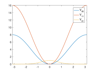
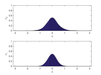
Figure 2: Top: diabatic potential surfaces for the test example (29). Bottom: equilibrium distribution on both surfaces.

The other test potential we take is given by

$$\left\{\begin{split}V_{00}&=a_{1}-b_{1}e^{-2(x-c_{1})^{2}};\\ V_{11}&=a_{2}-b_{2}e^{-2(x-c_{2})^{2}};\\ V_{01}&=V_{10}=d_{1}e^{-d_{2}x^{2}}.\end{split}\right.$$ (30)

$V_{00}$ and $V_{11}$ take their minima at $x=c_{1}$ and $x=c_{2}$ respectively, while the off-diagonal is peaked around $x=0$. In this model, the potential is asymmetric, and the two potentials have different minima, which also deviate from where the surface hopping is the most active due to the off-diagonal potential. These make this test model more challenging than the previous one. In this paper, we choose $a_{1}=5$, $a_{2}=5$, $b_{1}=5$, $b_{2}=4$, $c_{1}=0.3$, $c_{2}=-0.5$, $d_{1}=1$ and $d_{2}=2$. We plot the diabatic energy surfaces and the equilibrium distributions on each surface in Figure 3.

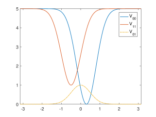
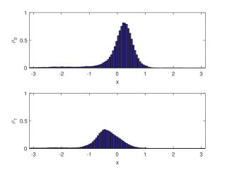
Figure 3: Left: diabatic potential surfaces for the test example (30). Right: equilibrium distribution on both surfaces.

For both potential examples, we test and compare the performances of numerical methods with the diagonal observable

$$\widehat{A}=\begin{bmatrix}e^{-{\widehat{q}}^{2}}&0\\ 0&e^{-{\widehat{q}}^{2}}\end{bmatrix},$$ (31)

and also the off-diagonal observable

$$\widehat{A}=\begin{bmatrix}0&e^{-{\widehat{q}}^{2}}\\ e^{-{\widehat{q}}^{2}}&0\end{bmatrix}.$$ (32)

IV.1 Tests for diagonal and off-diagonal observables with different $\Delta t$

Let us first use potential model (29) in order to compare with our previous method. We test the IS method and the HMM method for the number of beads $N=4$, $\beta=1$ and $\Delta t=\frac{1}{20}$, $\frac{1}{40}$, $\frac{1}{80}$ and $\frac{1}{160}$, which are compared with the direct simulation (DS) method. The tests are implemented with both the diagonal observable (31) and the off-diagonal observable (32).

In Figure 4, we plot the numerical results with the DS method. We observe that for the diagonal observable (31), we cannot clearly distinguish the performance with different time step sizes $\Delta t$ and all the tests are able to capture the thermal averages accurately, but for the off-diagonal observable (32), we need to take sufficiently small $\Delta t$ in order to obtain a reliable simulation. This confirms our observations in the previous paper.

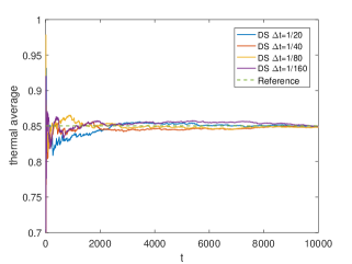
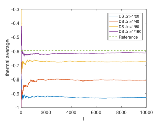
Figure 4: DS method with $N=4$, $\beta=1$ and various $\Delta t$ with potential model (29). Top: diagonal observable, the reference value is $0.850241$. Bottom: off-diagonal observable, the reference value is $-0.593497$.

In Figure 5, we plot the numerical results with the IS method and with the HMM method. We observe that for both observables (31) and (32), we are able to correctly approximate the thermal averages for various time step sizes $\Delta t$. For the HMM method, we choose a sufficiently large ratio of the macro/micro solver step sizes, $R={40}$, and we observe very similar results to those obtained by the IS method. This manifests a major improvement in the PIMD method for sampling off-diagonal observables.

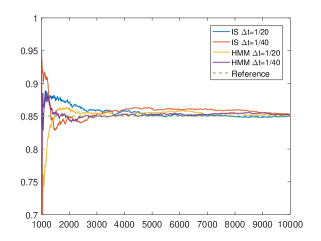
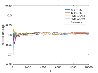
Figure 5: IS method and HMM method with $N=4$, $\beta=1$ and various $\Delta t$ with potential model (29), $R=40$ in the HMM method. Top: diagonal observable, the reference value is $0.850241$. Bottom: off-diagonal observable, the reference value is $-0.593497$.

We repeat the numerical tests for the off-diagonal observable (32), for a larger number of beads, $N=16$, $\beta=1$ and various time step sizes $\Delta t$, with the DS method and the HMM method. The tests for the diagonal observable are skipped since it is less challenging, and similar to the case when $N=4$, the DS method can already do a good job in those tests. In the HMM method, we choose the ratio of the macro/micro solver step sizes $R={40}$. The numerical results are plotted in Figure 6, where we observe that when $N$ is larger, the numerical errors of the DS method become also larger with same $\Delta t$. On the other hand, the HMM method give accurate approximation even for fairly large $\Delta t$.

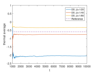
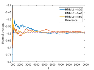
Figure 6: Off-diagonal observable with potential model (29). Top: DS method with $N=16$ and various $\Delta t$. Bottom: HMM method with the number of beads $N=16$ and various $\Delta t$. The reference value is $-0.593497$.

We remark that, these two tests above are presented in order to directly compare with the numerical results in Lu and Zhou (2017) and show the improvements. To rule out the possibility that the DS method only works for simple diagonal observables, we show in the following the test with another diagonal observable

$$\widehat{A}=\begin{bmatrix}e^{-{\widehat{q}}^{2}}&0\\ 0&-e^{-{\widehat{q}}^{2}}\end{bmatrix},$$ (33)

where the sign of the observable changes on different diabatic surfaces. We still use the potential model (29), and choose $N=4$, $\beta=1$. We test the DS method with $\Delta t=\frac{1}{20}$, $\frac{1}{40}$, $\frac{1}{80}$ and $\frac{1}{160}$, which are compared the IS method and the HMM method (with $R=40$) for $\Delta t=\frac{1}{20}$ and $\frac{1}{40}$, and the results are plotted in Figure 7. We observe that, unlike the tests with off-diagonal observables, the three methods give consistent numerical results even for large $\Delta t$, but the IS method and the HMM method give superior performances to the DS method.

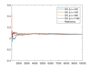
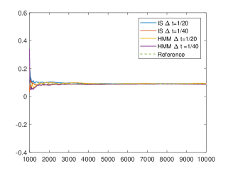
Figure 7: Diagonal observable (33) with potential model (29). Top: DS method with various $\Delta t$. Bottom: IS method and HMM method with various $\Delta t$. The reference value is $0.089901$.

Finally, we test with the second potential model (30) for the off-diagonal observable (32). The tests for the diagonal observable are skipped since it is less challenging, and similar to the tests with potential model (29), the DS method can already do a good job in those tests. For $N=4$ and $N=16$, we implement the HMM method with $R=40$, $\Delta t=\frac{1}{20}$ and $\frac{1}{40}$, which are compared with the DS method. The numerical results are plotted in Figure 8, where we observe that, the HMM method gives accurate approximation even for fairly large $\Delta t$, while the DS method gives rather poor accuracy.

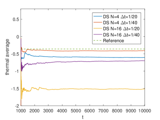
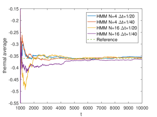
Figure 8: Off-diagonal observable with potential model (30). Top: DS method with $N=16$ and various $\Delta t$. Bottom: HMM method with the number of beads $N=16$ and various $\Delta t$. The reference value is $-0.360548$.

IV.2 Tests with different macro/micro time step ratios $R$

In the following, we focus on further exploration of numerical properties of the HMM method. We aim to test the sensitivity of the HMM method on two parameters, the number of beads $N$ and the macro/micro time step ratio $R$. In this section, we fix $N$ and test with various $R$, and we present the tests with various $N$ with a reasonably large $R$ in the next section.

In this section we aim to test the HMM method with different $R$ with a fairly large $\Delta t$, because the tests are obviously less challenging if $\Delta t$ is smaller. We will focus on the second potential model (30) as it is more challenging. We first fix $N=4$, $\beta=1$ and $\Delta t=\frac{1}{20}$, and test with the off-diagonal observable (32). We plot the results with $R=1$, $2$, $4$, $8$ and $16$, which is also compared with the reference value. We observe in Fig 9 (top) that even when $R=1$, the HMM method behaves much better than the DS method, and when $R=8$ and $16$, the HMM method behaves similarly, which suggest good convergence with respect to the choice of $R$.

We repeat the tests for $\beta=1$, $N=16$ and for $\beta=2$, $N=16$, where we observe similar trends as plotted in Fig 9 (middle and bottom). We conclude that when the IS method is no longer affordable since it has too many discrete states to explore, the HMM method with a reasonably large $R$ provides an alternative much faster way to sample off-diagonal observables.

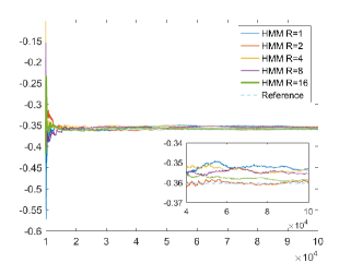
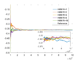
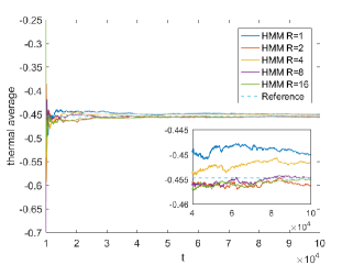
Figure 9: The HMM method for potential (30) with $T=10^{6}$, $\Delta t=\frac{1}{20}$ and various $R$ for the off-diagonal observable. Top: $\beta=1$, $N=4$, the reference values is $-0.360548$. Middle: $\beta=1$, $N=16$, the reference values is $-0.360548$. Bottom: $\beta=2$, $N=16$, the reference value is $-0.454771$.

At last, we carry out another comparison test between the DS method and the HMM method. We choose $N=4$, $\beta=1$, the tests are implemented with the second potential model (30) for the off-diagonal observable (32). In the DS method, we test with $\Delta t=\frac{1}{20}$, $\frac{1}{40}$, $\frac{1}{80}$ and $\frac{1}{160}$ till $T=10^{6}$. And the HMM method, we fixed $\Delta t=\frac{1}{20}$, but $R=1$, $2$, $4$ and $8$, so that $\Delta t/R$ in the HMM method matches $\Delta t$ in the DS method. This test is fair in terms of the numerical hopping frequency in both methods; we shall keep in mind though that the DS method takes finer time steps in integrating the trajectory of $(\boldsymbol{q},\boldsymbol{p})$, so it is more expensive. The mean squared errors of the empirical averages are defined as $\text{M.S.E.}=\text{Bias}^{2}+\text{Var}$, where Bias is calculated using the reference value and Var is estimated using the observed data and the effective sampling size. The M.S.E. for both methods are shown in Table 1, where we clearly observe that the performances of the HMM method are much better than the DS method.

DS	$\Delta t=\frac{1}{20}$	$\Delta t=\frac{1}{40}$	$\Delta t=\frac{1}{80}$	$\Delta t=\frac{1}{160}$
M.S.E.	6.5666e-2	2.6749e-3	9.7038e-4	8.4174e-4
HMM	$\frac{\Delta t}{R}=\frac{1}{20}$	$\frac{\Delta t}{R}=\frac{1}{40}$	$\frac{\Delta t}{R}=\frac{1}{80}$	$\frac{\Delta t}{R}=\frac{1}{160}$
M.S.E.	1.2851e-4	3.5028e-5	5.8980e-5	3.7058e-5

Table 1: Mean squared errors in the DS method and in the HMM method. In the HMM method, we fix $\Delta t=\frac{1}{20}$, but $R$ varies. The reference value is $-0.360548$.

IV.3 Tests with different $\beta_{N}$ for fixed $R$

In this section we aim to test the HMM method with various $N$ for a fixed but reasonably large $R$. We will again stick to the second potential model (30) with the off-diagonal observable (32). We fixed $\Delta t=\frac{1}{50}$, the final time $T=10^{4}$, $\beta=1$ and $R=16$, and test the performance of the HMM method with the number of beads $N=4$, $8$, $16$. We test with $\beta=1$, $R=32$ and with $\beta=2$ and $R=32$, and the results are plotted in Figure 10 (middle and bottom). We observe that, when $\beta=1$, for $R=16$ or $32$, the HMM method already gives accurate results. However, when $\beta=2$ and $R=32$, the numerical error is significantly larger for $N=4$. We believe it is mainly due to the asymptotic error, since the errors are reduced for $N=8$ and $N=16$, and become negligible for $N=32$.

Together with the previous section, we conclude that, the performance of the HMM method is more sensitive on the number of beads $N$ than to the time step ratio $R$. In practice, one needs to choose a proper $N$ to make sure the asymptotic error is acceptable and subsequently choose a reasonably large $R$, which is less constrained. We would like to remark that, choosing a sufficiently large $N$ might be a challenge, which is shared by most PIMD methods. Roughly speaking, larger $N$ is needed when the temperature is low ($\beta$ is large accordingly) and when profiles of the energy surfaces are complicated.

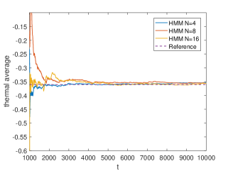
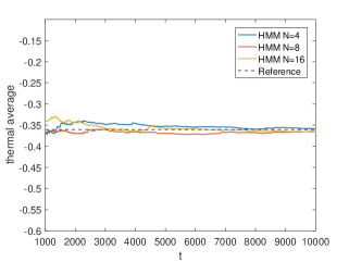
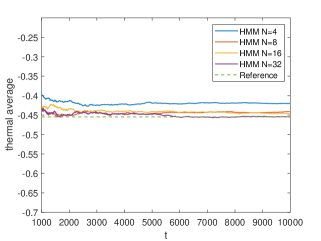
Figure 10: The HMM method for potential (30) with $\Delta t=\frac{1}{50}$, $T=10^{4}$ and various choice of $\beta$, $R$ and $N$. Top: $\beta=1$, $R=16$, the reference values is $-0.360548$. Middle: $\beta=1$, $R=32$, the reference values is $-0.360548$. Bottom: $\beta=2$, $R=32$, the reference value is $-0.454771$.

V Conclusion

Based on the theoretical analysis of the infinite swapping limit of the previously developed path-integral molecular dynamics with surface hopping method, we proposed in this work a multiscale integrator for the infinite swapping limit for sampling thermal equilibrium average of multi-level quantum systems. The efficiency of the proposed sampling scheme is greatly improved compared with the direct simulation of the PIMD-SH method. As for the future works, one immediate direction to explore is to combine the equilibrium sampling scheme with real time surface hopping dynamics to calculate dynamical correlation functions. In addition, we plan to test and further improve the proposed algorithms for realistic chemical applications with multidimensional potential surfaces.

Appendix A Ring polymer representation for two-level quantum systems

In this part, we present the details of the ring polymer representation of thermal averages as in (1) for two-level quantum systems, which have been rigorously derived in Lu and Zhou (2017). With the diabatic basis, we approximate the partition function by a ring polymer representation with $N$ beads

$$\operatorname{Tr}_{ne}[e^{-\beta\widehat{H}}]\approx\mathcal{Z}_{N}:=\frac{1}{(2\pi)^{dN}}\int_{{\mathbb{R}}^{2dN}}\,\mathrm{d}\boldsymbol{q}\,\mathrm{d}\boldsymbol{p}\times\\ \times\sum_{\boldsymbol{\ell}\in\{0,1\}^{N}}\exp(-\beta_{N}H_{N}(\boldsymbol{q},\boldsymbol{p},\boldsymbol{\ell})),$$ (34)

where $\beta_{N}=\beta/N$. The ring polymer that consists of $N$ beads is prescribed by the configuration $(\boldsymbol{q},\boldsymbol{p},\boldsymbol{\ell})\in{\mathbb{R}}^{dN}\times{\mathbb{R}}^{dN}\times\{0,1\}^{N}$.

For a given ring polymer with configuration $(\boldsymbol{q},\boldsymbol{p},\boldsymbol{\ell})$, the effective Hamiltonian $H_{N}(\boldsymbol{q},\boldsymbol{p},\boldsymbol{\ell})$ is given by

$$H_{N}(\boldsymbol{q},\boldsymbol{p},\boldsymbol{\ell})=\sum_{k=1}^{N}\langle\ell_{k}\rvert G_{k}\lvert\ell_{k+1}\rangle,$$ (35)

where we take the convention that $\ell_{N+1}=\ell_{1}$ and matrix elements of $G_{k}$, $k=1,\ldots,N$, are given by

$$\langle\ell\rvert G_{k}\lvert\ell^{\prime}\rangle=\frac{p^{2}_{k}}{2M}+\frac{M\left(q_{k}-q_{k+1}\right)^{2}}{2(\beta_{N})^{2}}\\ +\frac{V_{00}(q_{k})+V_{11}(q_{k})}{2}-\frac{1}{\beta_{N}}\ln\Bigl{(}\sinh\bigl{(}\beta_{N}\left\lvert V_{01}(q_{k})\right\rvert\bigr{)}\Bigr{)},$$ (36a)

for $$\ell\neq\ell^{\prime}$$, and the diagonal terms are given as

$$\langle\ell\rvert G_{k}\lvert\ell\rangle=\frac{p^{2}_{k}}{2M}+\frac{M\left(q_{k}-q_{k+1}\right)^{2}}{2(\beta_{N})^{2}}\\ +V_{\ell\ell}(q_{k})-\frac{1}{\beta_{N}}\ln\Bigl{(}\cosh\bigl{(}\beta_{N}\left\lvert V_{01}(q_{k})\right\rvert\bigr{)}\Bigr{)},$$ (36b)

where we have suppressed the $\boldsymbol{q}$ and $\boldsymbol{p}$ dependence in the notation of $G_{k}$. Here $G_{k}$ can be understood as the the contribution of $\langle q_{k}\rvert e^{-\beta_{N}\widehat{H}}\lvert q_{k+1}\rangle$ to the effective Hamiltonian $H_{N}$ in the ring polymer representation. The readers may refer to Lu and Zhou (2017) for the derivations.

For an observable $\widehat{A}$, under the ring polymer representation, we have

$$\operatorname{Tr}_{ne}[e^{-\beta\widehat{H}}\widehat{A}]\approx\frac{1}{(2\pi)^{dN}}\int_{{\mathbb{R}}^{2dN}}\,\mathrm{d}\boldsymbol{q}\,\mathrm{d}\boldsymbol{p}\sum_{\boldsymbol{l}\in\{0,1\}^{N}}\\ \times\exp(-\beta_{N}H_{N})W_{N}[A],$$ (37)

where the weight function associated to the observable is given by (recall that $\widehat{A}$ only depends on position by our assumption)

$$W_{N}[A](\boldsymbol{q},\boldsymbol{p},\boldsymbol{\ell})=\frac{1}{N}\sum_{k=1}^{N}\biggl{(}\langle\ell_{k}\rvert A(q_{k})\lvert\ell_{k}\rangle\\ -e^{\beta_{N}\langle\ell_{k}|G_{k}|\ell_{k+1}\rangle-\beta_{N}\langle\bar{\ell}_{k}\rvert G_{k}\lvert\ell_{k+1}\rangle}\langle\ell_{k}\rvert A(q_{k})\lvert\bar{\ell}_{k}\rangle\frac{V_{\ell_{k}\bar{\ell}_{k}}}{\lvert V_{\ell_{k}\bar{\ell}_{k}}\rvert}\biggr{)},$$ (38)

where we have introduced the short hand notation $\bar{\ell}_{k}=1-\ell_{k}$, i.e., $\bar{\ell}_{k}$ is the level index of the other potential energy surface than the one corresponds to $\ell_{k}$ in our two-level case. Similar as for the partition function, the ring polymer representation (37) replaces the quantum thermal average by an average over ring polymer configurations on the extended phase space ${\mathbb{R}}^{dN}\times{\mathbb{R}}^{dN}\times\{0,1\}^{N}$.

The ring polymer representation for a multi-level quantum system can be also constructed using the adiabatic basis Schmidt and Tully (2007); Lu and Zhou (2017), and much of the current work also extends to the ring polymer with the adiabatic basis. We will skip the details and leave to interested readers.

References

- Makri (1999) N. Makri, Annu. Rev. Phys. Chem. 50, 167 (1999).
- Stock and Thoss (2005) G. Stock and M. Thoss, Adv. Chem. Phys. 131, 243 (2005).
- Kapral (2006) R. Kapral, Annu. Rev. Phys. Chem. 57, 129 (2006).
- Feynman (1972) R. Feynman, Statistical Mechanics (Addison-Wesley, Reading, MA, 1972).
- Chandler and Wolynes (1981) D. Chandler and P. Wolynes, J. Chem. Phys. 74, 4078 (1981).
- Berne and Thirumalai (1986) B. Berne and D. Thirumalai, Ann. Rev. Phys. Chem. 37, 401 (1986).
- Markland and Manolopoulos (2008) T. E. Markland and D. E. Manolopoulos, J. Chem. Phys. 129, 024105 (2008).
- Ceriotti et al. (2010) M. Ceriotti, M. Parrinello, T. E. Markland, and D. E. Manolopoulos, J. Chem. Phys. 133, 124104 (2010).
- Schmidt and Tully (2007) J. R. Schmidt and J. C. Tully, J. Chem. Phys. 127, 094103 (2007).
- Shushkov et al. (2012) P. Shushkov, R. Li, and J. C. Tully, J. Chem. Phys. 137, 22A549 (2012).
- Lu and Zhou (2017) J. Lu and Z. Zhou, J. Chem. Phys. 146, 154110 (2017).
- Duke and Ananth (2016) J. Duke and N. Ananth, Faraday Discuss. 195, 253 (2016).
- Shakib and Huo (2017) F. Shakib and P. Huo, J. Phys. Chem. Lett. 8, 3073 (2017).
- Tully (1990) J. C. Tully, J. Chem. Phys. 93, 1061 (1990).
- Hammes-Schiffer and Tully (1994) S. Hammes-Schiffer and J. C. Tully, J. Chem. Phys. 101, 4657 (1994).
- Tully (1998) J. C. Tully, Faraday Discussions 110, 407 (1998).
- Shenvi et al. (2009) N. Shenvi, S. Roy, and J. C. Tully, Science 326, 829 (2009).
- Barbatti (2011) M. Barbatti, WIREs Comput. Mol. Sci. 1, 620 (2011).
- Subotnik and Shenvi (2011) J. E. Subotnik and N. Shenvi, J. Chem. Phys. 134, 024105 (2011).
- Subotnik et al. (2016) J. E. Subotnik, A. Jain, B. Landry, A. Petit, W. Ouyang, and N. Bellonzi, Annu. Rev. Phys. Chem. 67, 387 (2016).
- Lu and Zhou (ress) J. Lu and Z. Zhou, Math. Comp. (in press), arXiv:1602.06459.
- Lu and Zhou (2016) J. Lu and Z. Zhou, J. Chem. Phys. 145, 124109 (2016).
- Meyer and Miller (1979) H.-D. Meyer and W. Miller, J. Chem. Phys. 70, 3214 (1979).
- Stock and Thoss (1997) G. Stock and M. Thoss, Phys. Rev. Lett. 78, 578 (1997).
- Ananth and Miller III (2010) N. Ananth and T. F. Miller III, J. Chem. Phys. 133, 234103 (2010).
- Richardson and Thoss (2013) J. Richardson and M. Thoss, J. Chem. Phys. 139, 031102 (2013).
- Ananth (2013) N. Ananth, J. Chem. Phys. 139, 124102 (2013).
- Menzeleev et al. (2014) A. Menzeleev, F. Bell, and M. I. T. F., J. Chem. Phys. 140, 064103 (2014).
- Cotton and Miller (2015) S. Cotton and W. Miller, J. Phys. Chem. A 119, 12138 (2015).
- Hele and Ananth (2016) T. Hele and N. Ananth, Farad. Discuss. (2016).
- Liu (2016) J. Liu, J. Chem. Phys. 145, 204105 (2016).
- Moix et al. (2012) J. M. Moix, Y. Zhao, and J. Cao, Phys. Rev. B 85, 5412 (2012).
- Montoya-Castillo and Reichman (2017) A. Montoya-Castillo and D. R. Reichman, J. Chem. Phys. 146, 4107 (2017).
- Pavliotis and Stuart (2008) G. Pavliotis and A. Stuart, Multiscale methods: averaging and homogenization (Springer Science & Business Media, 2008).
- E (2011) W. E, Principles of multiscale modeling (Cambridge University Press, 2011).
- Prezhdo and Rossky (1997) O. V. Prezhdo and P. J. Rossky, J. Chem. Phys. 107, 825 (1997).
- E and Engquist (2003) W. E and B. Engquist, Commun. Math. Sci. 1, 87 (2003).
- Vanden-Eijnden (2003) E. Vanden-Eijnden, Commun. Math. Sci. 1, 385 (2003).
- E et al. (2007) W. E, B. Engquist, X. Li, W. Ren, and E. Vanden-Eijnden, Commun. Comput. Phys. 2, 367 (2007).
- Gear and Wells (1984) C. W. Gear and D. R. Wells, BIT Numerical Mathematics 24, 484 (1984).
- Tuckerman et al. (1990) M. Tuckerman, G. Martyna, and B. Berne, J. Chem. Phys. 93, 1287 (1990).
- Tuckerman and Berne (1991a) M. Tuckerman and B. Berne, J. Chem. Phys. 94, 1465 (1991a).
- Tuckerman and Berne (1991b) M. Tuckerman and B. Berne, J. Chem. Phys. 94, 6811 (1991b).
- Tuckerman and Berne (1991c) M. Tuckerman and B. Berne, J. Chem. Phys. 95, 8362 (1991c).
- Yu et al. (2016) T.-Q. Yu, J. Lu, C. F. Abrams, and E. Vanden-Eijnden, Proc. Natl. Acad. Sci. USA 113, 11744 (2016).
- Lu and Vanden-Eijnden (2017) J. Lu and E. Vanden-Eijnden, “Infinite swapping limit of parallel tempering as a stochastic switching process,” (2017), preprint.
- Dupuis et al. (2012) P. Dupuis, Y. Liu, N. Plattner, and J. D. Doll, Multi. Model. Simul. 10, 986 (2012).
- Gillespie (1977) D. Gillespie, J. Chem. Phys. 81, 2340 (1977).
- Leimkuhler and Matthews (2013) B. Leimkuhler and C. Matthews, J. Chem. Phys. 138, 174102 (2013).
- Lu and Spiliopoulos (2016) J. Lu and K. Spiliopoulos, “Multiscale integrators for stochastic differential equations and irreversible Langevin samplers,” (2016), preprint, arXiv:1606.09539.
- E et al. (2005) W. E, D. Liu, and E. Vanden-Eijnden, Comm. Pure App. Math. 58, 1544 (2005).
- Tao et al. (2010) M. Tao, H. Owhadi, and J. E. Marsden, Multi. Model. Simul. 8, 1269 (2010).