Balance control using both ZMP and COM height variations:
A convex boundedness approach

Abstract

Developments for 3D control of the center of mass (CoM) of biped robots are currently located in two local minima: on the one hand, methods that allow CoM height variations but only work in the 2D sagittal plane; on the other hand, nonconvex direct transcriptions of centroidal dynamics that are delicate to handle. This paper presents an alternative that controls the CoM in 3D via an indirect transcription that is both low-dimensional and solvable fast enough for real-time control. The key to this development is the notion of boundedness condition, which quantifies the capturability of 3D CoM trajectories.

I Introduction

Three-dimensional control of the center of mass follows in the wake of major achievements obtained in 2D locomotion with the linear inverted pendulum mode (LIPM) [1]. The core idea of the LIPM was to keep the CoM in a plane, which made the model tractable and paved the way for key discoveries, including the capture point [2] and capture-point based feedback control [3], subsequently applied in successful walking controllers [4, 5].

For a while, the ability to leverage vertical CoM motions seemed lost on the way, but recent developments showed a regain of interest for this capability [6, 7, 8]. All of them share a design choice that can be traced back to the seminal work of Pratt and Drakunov [9]: they interpolate CoM trajectories in a 2D sagittal plane for the inverted pendulum model (IPM) with fixed center of pressure. The key result of [9] is the conservation of the “orbital energy” of a CoM path, a variational principle that was later translated into a predictive controller in an equally inspirational study by Koolen et al. [7]. Ramos and Hauser [6] also noticed that the capture point, interpreted as point where to step, was a function of the CoM path, which they computed via a single shooting method. Interestingly, Hopkins et al. pointed out that vertical CoM motions is equivalent to turning the constant $\omega$ of the LIPM into a time-varying function $\omega(t)$ [10]. They brought to light a differential equation that this function must satisfy, and used it to compute back $\omega(t)$ from, once again, an a priori CoM-height trajectory.

Different as they may seem, the variational and point-where-to-step approaches are two instances of the same underlying concept: convergence of the system towards a steady state requires that its divergent component of motion stays bounded. Lanari et al. [11, 12] showed how the condition for this to happen involves an integral over the future trajectory of the system (one can see a similar integral in the orbital energy), which they named the boundedness condition.

The solution we explore in this study differs from existing approaches in that it considers $\omega(t)$ per se rather than as a result of CoM trajectories. This change of perspective is made possible by the derivation of the boundedness condition for the 3D IPM (Section II), which is then cast into an optimization problem for 2D and 3D control of the CoM (Sections III and IV). The resulting predictive controller is implemented and tested in Section V.

II Boundedness condition of the IPM

The equation of motion of the inverted pendulum model is:

$$\ddot{\bm{c}}(t)=\lambda(t)(\bm{c}(t)-\bm{r}(t))+\bm{g}$$ (1)

where $\bm{c}$ is the center of mass (CoM) of the robot, $\bm{r}$ is the center of pressure (CoP) under its contacting foot, and $\bm{g}=-g\bm{e}_{z}$ is the gravity vector. The quantity $\lambda$ has the unit of a stiffness. It must be positive $\lambda\geq 0$ by unilaterality of contact, while the CoP $\bm{r}$ always belongs to the contact area.

II-A Divergent component of motion

To alleviate calculations, let us formulate the divergent component of motion [13] of this model as a velocity rather than a point:

$$\bm{\xi}(t)=\dot{\bm{c}}(t)-\dot{\bm{r}}(t)+\omega(t)(\bm{c}(t)-\bm{r}(t))$$ (2)

where $\omega(t)$ is a solution to the differential equation [10]:

$$\dot{\omega}=\omega^{2}-\lambda$$ (3)

The quantity $\omega$ has the unit of a damping. The interest of its differential equation appears when differentiating the divergent component of motion:

$$\dot{\bm{\xi}}=(\lambda+\dot{\omega})(\bm{c}-\bm{r})+\omega(\dot{\bm{c}}-\dot{\bm{r}})+\bm{g}-\ddot{\bm{r}}=\omega\bm{\xi}+\bm{g}-\ddot{\bm{r}}$$ (4)

The solution to this first-order differential equation is:

$$\bm{\xi}(t)=\left(\bm{\xi}(0)+\int_{0}^{t}e^{-\Omega(\tau)}(\bm{g}-\ddot{\bm{r}}(\tau)){\rm d}{\tau}\right)e^{\Omega(t)}$$ (5)

where $\Omega$ is the antiderivative of $\omega$ such that $\Omega(0)=0$. In the LIPM where the damping $\omega$ is a constant, $\Omega(t)=\omega t$ and this equation is equivalent to the well-known capture point dynamics [13].

To be viable [14], the trajectory of the system must be bounded, which implies that the above expression does not diverge despite its exponential factor. This necessary condition for viability is known as the boundedness condition [11, 12], and is written here:

$$\int_{0}^{\infty}(\ddot{\bm{r}}(t)-\bm{g})e^{-\Omega(t)}{\rm d}{t}=\bm{\xi}(0)$$ (6)

Note how this requirement involves both the CoP trajectory $\bm{r}(t)$ and stiffness trajectory $\lambda(t)$: the former is integrated through $\ddot{\bm{r}}(t)$, while the latter is embedded in $\Omega(t)$.

II-B Decoupling of the boundedness constraint

Let us express all coordinates in the inertial frame depicted in Figure 1. In what follows, we will use the subscript $\mathrm{i}$ (“initial”) to indicate values at $t=0$, and $\mathrm{f}$ (“final”) for stationary values obtained as $t\to\infty$. The origin of the inertial frame is taken at the stationary CoP position $\bm{r}_{\mathrm{f}}=\bm{0}$ where we want the robot to stop. The stationary CoM position is then $\bm{c}_{\mathrm{f}}=z_{\mathrm{f}}\bm{e}_{z}$, with $z_{\mathrm{f}}$ the desired stationary CoM height. The two vectors $\bm{e}_{x}$ and $\bm{e}_{y}$ are horizontal (i.e. orthogonal to gravity), and $\bm{e}_{x}$ is chosen aligned with the horizontal projection of $\bm{r}_{\mathrm{f}}-\bm{c}_{\mathrm{i}}$.

In reality, the center of pressure always lies on the contact surface between the robot and its environment. Therefore, CoPs $\bm{r}$ output by our controller must satisfy the feasibility condition of lying on the contact surface. Denoting by $\bm{n}$ the contact normal, this means that $\bm{r}$ and all its derivatives are orthogonal to $\bm{n}$; in particular, $\ddot{\bm{r}}(t)\cdot\bm{n}=0$ at all times. Taking the dot product of Equation (6) with $\bm{n}$ then yields:

$$\int_{0}^{\infty}e^{-\Omega(t)}{\rm d}{t} =\frac{\dot{\bar{z}}_{\mathrm{i}}+\omega_{\mathrm{i}}\bar{z}_{\mathrm{i}}}{g}$$ (7)

where $\bar{z}\stackrel{{\scriptstyle\mathrm{def}}}{{=}}{(\bm{c}\cdot\bm{n})}/{(\bm{e}_{z}\cdot\bm{n})}$ is the height of the vertical projection of $\bm{c}$ onto the contact surface.

Let us now define $\bm{p}(t)\stackrel{{\scriptstyle\mathrm{def}}}{{=}}\begin{bmatrix}r_{x}(t)&r_{y}(t)\end{bmatrix}$ and $\bar{\bm{c}}_{\mathrm{i}}\stackrel{{\scriptstyle\mathrm{def}}}{{=}}\begin{bmatrix}x_{\mathrm{i}}&y_{\mathrm{i}}\end{bmatrix}$ the horizontal projections of the CoP and CoM, respectively. The horizontal projection of Equation (6) is:

$$\int_{0}^{\infty}\ddot{\bm{p}}(t)e^{-\Omega(t)}{\rm d}{t}=(\dot{\bar{\bm{c}}}_{\mathrm{i}}-\dot{\bm{p}}_{\mathrm{i}})+\omega_{\mathrm{i}}(\bar{\bm{c}}_{\mathrm{i}}-\bm{p}_{\mathrm{i}})$$ (8)

A double integration by parts of the left hand side of this equation yields:

$$\int_{0}^{\infty}\ddot{\bm{p}}(t)e^{-\Omega(t)}{\rm d}{t}=\int_{0}^{\infty}\bm{p}(t)\lambda(t)e^{-\Omega(t)}{\rm d}{t}-(\dot{\bm{p}}_{\mathrm{i}}+\omega_{\mathrm{i}}\bm{p}_{\mathrm{i}})$$

Combining these last two equations, we obtain a temporal formulation of the boundedness condition with separate gravity and CoP components:

$$\int_{0}^{\infty}e^{-\Omega(t)}{\rm d}{t} =\frac{\dot{\bar{z}}_{\mathrm{i}}+\omega_{\mathrm{i}}\bar{z}_{\mathrm{i}}}{g}$$ (9)

$$\int_{0}^{\infty}\bm{p}(t)\lambda(t)e^{-\Omega(t)}{\rm d}{t} =\dot{\bar{\bm{c}}}_{\mathrm{i}}+\omega_{\mathrm{i}}\bar{\bm{c}}_{\mathrm{i}}$$ (10)

Equations (9)–(10) are equivalent to (6) as $(\bm{e}_{x},\bm{e}_{y},\bm{n})$ is a (non-orthogonal) basis of the 3D Euclidean space.

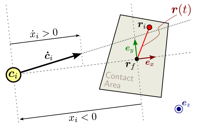
Figure 1: Definition of the inertial frame $(\bm{e}_{x},\bm{e}_{y},\bm{e}_{z})$. The frame is rooted at the stationary CoP location $\bm{r}_{f}$. The instantaneous CoM location is denoted by $\bm{c}_{\mathrm{i}}$. Both vectors $\bm{e}_{x}$ and $\bm{e}_{y}$ lie in the horizontal plane, and $\bm{e}_{x}$ is aligned with the (horizontal projection of the) desired direction of motion $\bm{r}_{\mathrm{f}}-\bm{c}_{\mathrm{i}}$.

In the familiar setting of the LIPM, the first equation boils down to:

$$\int_{0}^{\infty}e^{-\omega t}{\rm d}{t}=\frac{1}{\omega}=\frac{0+\omega z}{g}\Longleftrightarrow\omega=\sqrt{\frac{g}{z}}$$ (11)

Meanwhile, taking $\bm{p}=0$ in the second one implies that the traditional LIPM capture point is located at $\bm{r}_{f}$. This observation illustrates how the boundedness condition (9)–(10) encompasses the well-known model.

II-C Change of variable

Define the adimensional quantity $s(t)=e^{-\Omega(t)}$. This variable ranges from $1$ when $t=0$ to $0$ as $t\to\infty$, and its time derivatives are:

$$\dot{s}(t) =-\omega(t)s(t)$$ (12)

$$\ddot{s}(t) =\lambda(t)s(t)$$ (13)

Thanks to the bijective mapping between $s$ and $t$, we can characterize $\omega$ and $\lambda$ indistinctly as functions of $s$ or $t$. Let us choose the former, and denote by $(\cdot)^{\prime}$ derivatives with respect to $s$. For instance, $\omega(t)=\omega(s(t))$ implies that:

$$\frac{{\rm d}{\omega}}{{\rm d}{t}}(t)=\frac{{\rm d}{s}}{{\rm d}{t}}(t)\frac{{\rm d}{\omega}}{{\rm d}{s}}(s(t))\Longrightarrow\dot{\omega}=\dot{s}\omega^{\prime}=-s\omega\omega^{\prime}$$ (14)

where we eventually omit arguments $\square(t)$ and $\square(s(t))$ for brevity. Applying the chain rule similarly yields:

$${\rm d}{t} =\frac{{\rm d}{s}}{\dot{s}}=-\frac{{\rm d}{s}}{\omega(s)s}$$ (15)

$$\lambda =\omega^{2}-\dot{\omega}=\omega(\omega+s\omega^{\prime})=\omega(s\omega)^{\prime}$$ (16)

We can therefore formulate the boundedness condition (9)–(10) in terms of the new variable $s$ as:

$$\int_{0}^{1}\frac{1}{\omega(s)}{\rm d}{s} =\frac{\dot{\bar{z}}_{\mathrm{i}}+\omega_{\mathrm{i}}\bar{z}_{\mathrm{i}}}{g}$$ (17)

$$\int_{0}^{1}\bm{p}(s)(s\omega)^{\prime}{\rm d}{s} =\dot{\bar{\bm{c}}}_{\mathrm{i}}+\omega_{\mathrm{i}}\bar{\bm{c}}_{\mathrm{i}}$$ (18)

With this change of variable, infinite integrals over time solutions $\omega(t),\bm{p}(t)$ are turned into finite integrals over functions $\omega(s),\bm{p}(s)$ of the new variable $s$. This approach bears a close resemblance to the recently proposed concept of spatial quantization [15].

III Sagittal 2D Balance with Fixed CoP

Let us consider first the case of 2D stabilization in the plane $(\bm{e}_{x},\bm{e}_{z})$ with a fixed CoP. Since $r_{x}=0$, the boundedness condition becomes:

$$\omega_{\mathrm{i}} =-\frac{\dot{x}_{\mathrm{i}}}{x_{\mathrm{i}}}$$ (19)

$$\dot{z}_{\mathrm{i}}+\omega_{\mathrm{i}}z_{\mathrm{i}} =g\int_{0}^{1}\frac{1}{\omega(s)}{\rm d}{s}$$ (20)

Equation (19) implies via (5) that $\dot{x}=-\omega x$, which integrates to $x(t)=x_{\mathrm{i}}e^{-\Omega(t)}=x_{\mathrm{i}}s(t)$. We see how, in 2D balance control, the coordinates $x$ and $s$ are proportional. Interpolation over $x$ [7, 9] is therefore equivalent to interpolation over $s$, and one can recognize in (20) the same principle as the conservation of orbital energy [9]. The benefit of using $s$ rather than $x$ will appear when we move to 3D control.

III-A Viability condition

The viability condition $z_{\text{crit}}\geq 0$ derived in [7] for $\lambda\geq 0$ can be seen as a consequence of (20). Indeed, the lower-bounding profile $\underline{\lambda}=0$ corresponds to $(s\underline{\omega})^{\prime}=0$, that is to say, $s\underline{\omega}=\omega_{\mathrm{i}}$. It follows that:

$$\int_{0}^{1}\frac{{\rm d}{s}}{\omega(s)}\geq\int_{0}^{1}\frac{{\rm d}{s}}{\underline{\omega}(s)}=\int_{0}^{1}\frac{s}{\omega_{\mathrm{i}}}{\rm d}{s}=\frac{1}{2\omega_{\mathrm{i}}}$$ (21)

$$z_{\text{crit}}=z_{\mathrm{i}}+\frac{\dot{z}_{\mathrm{i}}}{\omega_{\mathrm{i}}}-\frac{g}{2\omega_{\mathrm{i}}^{2}}=\frac{g}{\omega_{\mathrm{i}}}\left[\int_{0}^{1}\frac{{\rm d}{s}}{\omega(s)}-\frac{1}{2\omega_{\mathrm{i}}}\right]\geq 0$$ (22)

In practice, biped robots cannot exert arbitrary large contact forces, and tend to break contact when ground pressure becomes too low. To reflect this, we will thereafter consider the stricter feasibility condition $\lambda\in[\lambda_{\text{min}},\lambda_{\text{max}}]$. The corresponding viability condition can be derived in a similar fashion by considering lower- and upper-bounding profiles:

$$\dot{z}_{\mathrm{i}}+\omega_{\mathrm{i}}z_{\mathrm{i}} \leq\frac{g}{\lambda_{\text{max}}}\left[\omega_{\mathrm{i}}+\sqrt{\frac{\lambda_{\text{max}}-\lambda_{\text{min}}}{\lambda_{\text{min}}}}\sqrt{\lambda_{\text{max}}-\omega_{\mathrm{i}}^{2}}\right]$$ (23)

$$\dot{z}_{\mathrm{i}}+\omega_{\mathrm{i}}z_{\mathrm{i}} \geq\frac{g}{\lambda_{\text{min}}}\left[\omega_{\mathrm{i}}-\sqrt{\frac{\lambda_{\text{max}}-\lambda_{\text{min}}}{\lambda_{\text{max}}}}\sqrt{\omega_{\mathrm{i}}^{2}-\lambda_{\text{min}}}\right]$$ (24)

III-B Computing feasible $\omega$ solutions

Let us partition the interval $[0,1]$ into $N$ fixed segments $0=s_{0}<s_{1}<\ldots<s_{N}=1$, for instance $s_{j}=j/N$. We compute solutions to the boundedness condition where $\lambda(s)$ is piecewise constant over this subdivision, that is, $\forall s\in[s_{j},s_{j+1}],\lambda(s)=\lambda_{j}$. Define:

$$\varphi(s) \stackrel{{\scriptstyle\mathrm{def}}}{{=}}s^{2}\omega^{2} \Delta_{j} \stackrel{{\scriptstyle\mathrm{def}}}{{=}}s_{j+1}^{2}-s_{j}^{2}$$ (25)

Remarking that $\varphi^{\prime}=2s\lambda$ from Equation (16), we can directly compute $\varphi(s)$ for $s\in[s_{j},s_{j+1}]$ as:

$$\varphi(s)=\sum_{k=0}^{j-1}\lambda_{k}\Delta_{k}+\lambda_{j}(s^{2}-s_{j}^{2})$$ (26)

In what follows, we use the shorthand $\varphi_{j}=\varphi(s_{j})$.

We can now calculate the right-hand side of the boundedness condition (20):

$$\int_{0}^{1}\frac{{\rm d}{s}}{\omega(s)} =\sum_{j=0}^{N-1}\int_{s_{j}}^{s_{j+1}}\frac{s{\rm d}{s}}{\sqrt{\varphi_{j}+\lambda_{j}(s^{2}-s_{j}^{2})}}$$ (27)

$$=\sum_{j=0}^{N-1}\int_{0}^{\Delta_{j}}\frac{{\rm d}{v}}{2\sqrt{\varphi_{j}+\lambda_{j}v}}$$ (28)

$$=\sum_{j=0}^{N-1}\frac{1}{\lambda_{j}}\left[\sqrt{\varphi_{j}+\lambda_{j}\Delta_{j}}-\sqrt{\varphi_{j}}\right]$$ (29)

$$=\sum_{j=0}^{N-1}\frac{\Delta_{j}}{\sqrt{\varphi_{j+1}}+\sqrt{\varphi_{j}}}$$ (30)

Note that the latter expression is convex in the variables $\varphi_{1},\ldots,\varphi_{N}$ (by definition $\varphi_{0}=0$), as shown in Appendix -A.

Besides boundedness, solutions should enforce three conditions:

• Feasibility: $\lambda_{\text{min}}\leq\lambda\leq\lambda_{\text{max}}$, expressed linearly in terms of $\varphi$ as $\Delta_{j}\lambda_{\text{min}}\leq\varphi_{j+1}-\varphi_{j}\leq\Delta_{j}\lambda_{\text{max}}$;

• Initial state: $\omega$ should be equal to $\omega_{\mathrm{i}}$ at the initial index $s=1$, that is to say, $\varphi_{N}=\omega_{\mathrm{i}}^{2}$;

• Stationary state: a stationary COM height $z_{\mathrm{f}}$ can also be specified via $\varphi_{1}=\Delta_{0}g/z_{\mathrm{f}}$, or similarly a range of heights $z_{\text{min}}\leq z_{\mathrm{f}}\leq z_{\text{max}}$ used to approximate kinematic reachability.

Wrapping all four conditions together and adding a regularizing cost function over variations of $\lambda$, we obtain Optimization Problem 1. This problem is “almost” a quadratic program: it has a quadratic cost function and linear constraints, except for Equation (33) which is a one-dimensional nonlinear equality constraint.

III-C Model predictive control for 2D balance

Solving Problem 1 can be done fast enough for the control loop, on the scale of 1–3 ms using a general-purpose nonlinear solver (see Section V). At each control cycle, we compute the optimum $\varphi_{1}^{*},\ldots,\varphi_{N}^{*}$ of the problem and extract its initial stiffness via:

$$\lambda_{\mathrm{i}}^{*}=\frac{\omega_{\mathrm{i}}^{2}-\varphi_{N-1}^{*}}{\Delta_{N-1}}$$ (31)

This value is then sent as reference to the lower-level leg and attitude controllers until the next control cycle. In the standard model-predictive fashion, the rest of the optimal trajectory is discarded. As a matter of fact, the trajectories $\omega(s)$ and $\lambda(s)$ are never explicitly computed, let alone their time counterparts. The operation is possible (see Appendix -B) but not necessary for control. Compared to the controller from [7], this solution enforces feasibility constraints $\lambda_{\text{min}}\leq\lambda\leq\lambda_{\text{max}}$ a priori, as opposed to an a posteriori clipping that may cause free-falling phases in the output trajectory.

Optimization Problem 1 2D Balance Control

$$\underset{\varphi_{1},\ldots,\varphi_{N}}{\text{minimize }} \sum_{j=1}^{N-1}\left[\frac{\varphi_{j+1}-\varphi_{j}}{\Delta_{j}}-\frac{\varphi_{j}-\varphi_{j-1}}{\Delta_{j-1}}\right]^{2}$$ (32)

subject to $$\sum_{j=0}^{N-1}\frac{\Delta_{j}}{\sqrt{\varphi_{j+1}}+\sqrt{\varphi_{j}}}=\frac{\dot{\bar{z}}_{\mathrm{i}}+\omega_{\mathrm{i}}\bar{z}_{\mathrm{i}}}{g}$$ (33)

$$\varphi_{N}=\omega_{\mathrm{i}}^{2}$$ (34)

$$\forall j,\ \lambda_{\text{min}}\Delta_{j}\leq\varphi_{j+1}-\varphi_{j}\leq\lambda_{\text{max}}\Delta_{j}$$ (35)

$$\varphi_{1}=\Delta_{0}g/z_{\mathrm{f}}$$ (36)

IV 3D Balance

In 3D balance where the initial velocity $\dot{\bm{c}}_{\mathrm{i}}$ is not necessarily coplanar with the stationary state, the CoP cannot be fixed and the initial damping $\omega_{\mathrm{i}}$ is not determined by Equation (19) any more. The latter is replaced by a more general condition over CoP trajectories:

$$\int_{0}^{1}\bm{p}(s)(s\omega)^{\prime}{\rm d}{s}=\dot{\bar{\bm{c}}}_{i}+\omega_{\mathrm{i}}\bar{\bm{c}}_{\mathrm{i}}$$ (37)

Subject to the feasibility conditions:

$$\mathbf{A}\bm{p}\leq\bm{b}$$ (38)

where the matrix $\mathbf{A}$ and vector $\bm{b}$ form the halfspace-representation of the contact polygon. This polygon is readily computed from contact geometry. For example, a rectangular contact $|(\bm{p}\cdot\bm{e}_{w})|\leq W$, $|(\bm{p}\cdot\bm{e}_{h})|\leq H$ has four inequalities:

$$\pm\begin{bmatrix}(\bm{e}_{x}\cdot\bm{e}_{w})&(\bm{e}_{y}\cdot\bm{e}_{w})\\ (\bm{e}_{x}\cdot\bm{e}_{h})&(\bm{e}_{y}\cdot\bm{e}_{h})\end{bmatrix}\bm{p}\leq\begin{bmatrix}W\\ H\end{bmatrix}$$ (39)

IV-A Computing feasible CoP solutions

The structure of Equation (37) suggests a particular solution: let us take $\bm{p}(s)=\bm{p}_{\mathrm{i}}f(s\omega)$, where:

• $f(\omega_{\mathrm{i}})=1$: initially, the CoP is located at $\bm{r}_{\mathrm{i}}$;

• $f(0)=0$: eventually, the CoP is located at $\bm{r}_{\mathrm{f}}$;

• $f$ is increasing: we exclude solutions where the CoP goes back and forth, that we deem suboptimal;

• $f$ is integrable: let $F$ denote its antiderivative such that $F(0)=0$. It is positive by monotonicity of $f$.

With this choice, the boundedness condition (37) becomes

$$\bm{p}_{\mathrm{i}}=\frac{\dot{\bar{\bm{c}}}_{\mathrm{i}}+\omega_{\mathrm{i}}\bar{\bm{c}}_{\mathrm{i}}}{F(\omega_{\mathrm{i}})}$$ (40)

By monotonicity of $f$, the CoP trajectory is feasible if and only if its initial position $\bm{p}_{\mathrm{i}}$ satisfies the feasibility condition (38). Considering (40), this can be written:

$$\bm{b}F(\omega_{\mathrm{i}})-(\mathbf{A}\bar{\bm{c}}_{\mathrm{i}})\omega_{\mathrm{i}}\geq\mathbf{A}\dot{\bar{\bm{c}}}_{\mathrm{i}}$$ (41)

Compared to the previous fixed-CoP setting where $\omega_{\mathrm{i}}$ was fully determined, we see how the relaxed polygonal constraint $\mathbf{A}\bm{p}\leq\bm{b}$ now frees a range of possible choices for $\omega_{\mathrm{i}}$. At this stage, one can explore different CoP strategies via the choice of a (preferably convex) function $F$. Let us focus on the example of a power law, i.e. for some $k>1$:

$$f(s\omega)=\left(s\frac{\omega}{\omega_{\mathrm{i}}}\right)^{k-1}\Longrightarrow F(\omega_{\mathrm{i}})=\frac{\omega_{\mathrm{i}}}{k}$$ (42)

Equation (41) simplifies to:

$$\left(\frac{\bm{b}}{k}-\mathbf{A}\bar{\bm{c}}_{\mathrm{i}}\right)\omega_{\mathrm{i}}\geq\mathbf{A}\dot{\bar{\bm{c}}}_{\mathrm{i}}$$ (43)

Each line of this vector inequality provides a lower or upper bound on $\omega_{\mathrm{i}}$, depending on the sign of the factor in front of it. These inequalities can then be summed up as $\omega_{\mathrm{i},\text{min}}\leq\omega_{\mathrm{i}}\leq\omega_{\mathrm{i},\text{max}}$. Note that this computation is only carried out once from the initial state, i.e. it is not part of the following numerical optimization.

Optimization Problem 2 3D Balance Control

$$\underset{\varphi_{1},\ldots,\varphi_{N}}{\text{minimize }} \sum_{j=1}^{N-1}\left[\frac{\varphi_{j+1}-\varphi_{j}}{\Delta_{j}}-\frac{\varphi_{j}-\varphi_{j-1}}{\Delta_{j-1}}\right]^{2}$$ (32)

subject to $$\sum_{j=0}^{N-1}\frac{\Delta_{j}}{\sqrt{\varphi_{j+1}}+\sqrt{\varphi_{j}}}-\frac{\bar{z}_{\mathrm{i}}}{g}\sqrt{\varphi_{N}}=\frac{\dot{\bar{z}}_{\mathrm{i}}}{g}$$ (44)

$$\omega_{\mathrm{i},\text{min}}^{2}\leq\varphi_{N}\leq\omega_{\mathrm{i},\text{max}}^{2}$$ (45)

$$\forall j,\ \lambda_{\text{min}}\Delta_{j}\leq\varphi_{j+1}-\varphi_{j}\leq\lambda_{\text{max}}\Delta_{j}$$ (35)

$$\varphi_{1}=\Delta_{0}g/z_{\mathrm{f}}$$ (36)

By definition of $\varphi$, $\omega_{\mathrm{i}}$ is equal to $\sqrt{\varphi_{N}}$, so that bounds on $\omega$ are mapped directly into the optimization as $\omega_{\mathrm{i},\text{min}}^{2}\leq\varphi_{N}\leq\omega_{\mathrm{i},\text{max}}^{2}$. However, previously $\omega_{\mathrm{i}}$ also appeared in the right-hand side of the nonlinear equality constraint (33). In 3D, this constraint becomes:

$$\sum_{j=0}^{N-1}\frac{\Delta_{j}}{\sqrt{\varphi_{j+1}}+\sqrt{\varphi_{j}}}-\frac{\bar{z}_{\mathrm{i}}}{g}\sqrt{\varphi_{N}}=\frac{\dot{\bar{z}}_{\mathrm{i}}}{g}$$ (46)

Both the function $x\mapsto-\sqrt{x}$ and the expression from Equation (30) are convex, therefore this new expression is convex as well. Wrapping up these developments, we obtain Optimization Problem 2.

IV-B Model predictive control for 3D balance

Our pipeline for 3D balance is the same as in Section III. Once the optimal solution $\varphi_{1}^{*},\ldots,\varphi_{N}^{*}$ of Problem 2 is found, stiffness and CoP are extracted as:

$$\omega_{\mathrm{i}}^{*} =\sqrt{\varphi_{N}^{*}} \lambda_{\mathrm{i}}^{*} =\frac{\varphi_{N}^{*}-\varphi_{N-1}^{*}}{\Delta_{N-1}} \bm{p}_{\mathrm{i}}^{*} =\frac{\dot{\bar{\bm{c}}}_{\mathrm{i}}+\bar{\bm{c}}_{\mathrm{i}}\omega_{\mathrm{i}}^{*}}{F(\omega_{\mathrm{i}}^{*})}$$ (47)

In the case of the power law (42), the CoP solution becomes:

$$\bm{p}^{*}=k\left[\bm{p}_{\mathrm{i}}+\frac{\dot{\bm{p}}_{\mathrm{i}}}{\omega_{\mathrm{i}}^{*}}\right]$$ (48)

Interestingly, we recognize here the expression of the capture-point feedback control law [3, 5, 13], under the usual requirement that $k>1$, even though we are in the context of 3D balance where $\lambda$ and $\omega$ are time-varying.

Problem 2 is solved as fast as its 2D counterpart, on the scale of 1–3 ms, but it is able to cope with both sagittal and lateral velocity compensation. Its solutions tend to be flatter thanks to a wider range of CoP positions. As a matter of fact, by trying to keep the stiffness $\lambda$ as constant as possible, Problem 2 generates a hierarchical strategy: CoP variations are used first; then, if need be, CoM height variations are resorted to. This behavior is depicted in Figure 2.

IV-C Discussion

CoM trajectory generation using 6D contacts is a notoriously nonconvex problem due to angular momentum. Even when a linear model is used and angular momentum is kept constant [5], nonconvexity lingers in feasibility inequality constraints [16]. Nonlinear optimal control has been explored on direct transcriptions of this problem using e.g. multiple shooting [17]; however, our experience in [18] met with frequent solver failures caused by local optimum switches, which required dedicated countermeasures. To avoid such switches, Ponton et al. [19] proposed a convex relaxation of the direct transcription of centroidal dynamics by bounding the convex and concave parts of the angular momentum.

Compared to these previous works, the study we propose here relies on an indirect transcription, i.e. optimization variables are neither the CoM position nor its derivatives. To reduce further the dimension of the problem, we made the CoP trajectory a consequence $\bm{p}(s)=\bm{p}_{\mathrm{i}}f(s\omega)$ of the damping profile $\omega$, as opposed to e.g. a shooting method where $\bm{p}$ and $\omega$ would be optimized jointly. Choosing a linear CoP trajectory also impacts the existence of feasible solutions, for instance when the feedback gain $k$ is too large. An effect that is by the way also present in all capture-point feedback controllers [3, 4, 5, 10, 20].

Compared to e.g. [16, 17, 18], we did not explicitly model frictional constraints in the present study. We observe however, as noted in [7], that the friction force is maximal at the beginning of the balancing trajectory. It can therefore be constrained (if needed) within the presented framework via additional instantaneous CoP inequalities (38).

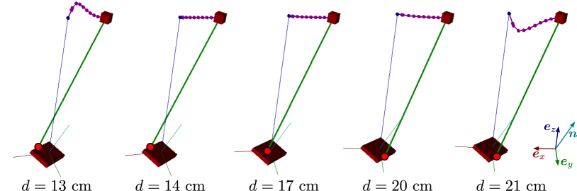
Figure 2: Saturation behavior of the 3D balance controller. The horizontal distance from CoM to contact is denoted by $d$, $\bm{n}$ is the contact normal and red discs indicate the initial CoP. The controller keeps the CoM trajectory as close as possible to a LIPM via CoP variations. When this is not enough, height variations are resorted to for additional braking.

V Stepping experiments

We implemented both balance controllers and evaluated them in pymanoid, an extension of OpenRAVE for humanoid robotics. Optimization problems were formulated with a spatial discretization $s_{j}=j/N$ with $N=10$. They were subsequently solved using the IPOPT solver, with Jacobians and Hessians computed by automatic differentiation via CasADi. Note that IPOPT is a general-purpose nonlinear solver designed for large-scale problems, while the problems at hand are small and have additional structure. A dedicated solver can leverage this structure for improved performance [21].

We ran a benchmark over randomized states and contact locations for Problems 1 and 2. Both solvers were fed the same initial states, and sampling was biased toward viable states using the proxy distribution $z_{\text{crit}}\sim\frac{1}{2}z_{\mathrm{f}}+\sigma_{z}{\cal U}([0,1])$. On an Intel Core i7-6500U CPU @ 2.50 Ghz, computation times were identical: $1.8\pm 0.7$ ms and $1.7\pm 0.6$ ms for the 2D and 3D problem, respectively (averages and standard deviations over $10000$ control cycles aggregated over 225 launches from different initial states). These times can be improved by two orders of magnitude using the dedicated solver introduced in the extension [21] of the present work.

We next considered a push recovery scenario for an HRP-4 humanoid evolving in a 3D model of an A350 aircraft under construction. Due to e.g. an unexpected collision, or slippage over a ground obstacle that is only detected after momentum has built up, the robot is imparted with an initial velocity of 1.4 m s^-1. Although hand contacts would be equally important in such scenarios, we focus here on the stance leg trajectory. First, a foothold is chosen on the fuselage as the kinematically reachable location with the lowest tilting. The velocity in the resulting frame (Figure 1) consists of roughly 1.3 m s^-1 in the desired direction of motion $\bm{e}_{x}$, 0.2 m s^-1 in the lateral direction $\bm{e}_{y}$ and 0.5 m s^-1 along the vertical $\bm{e}_{z}$. We confirmed that the robot is able to stop in 1.5 s using using the CoP strategy (42) with $k=2$ and a 10 cm CoM height variation. The scenario is depicted in Figure 3 and in the accompanying video.

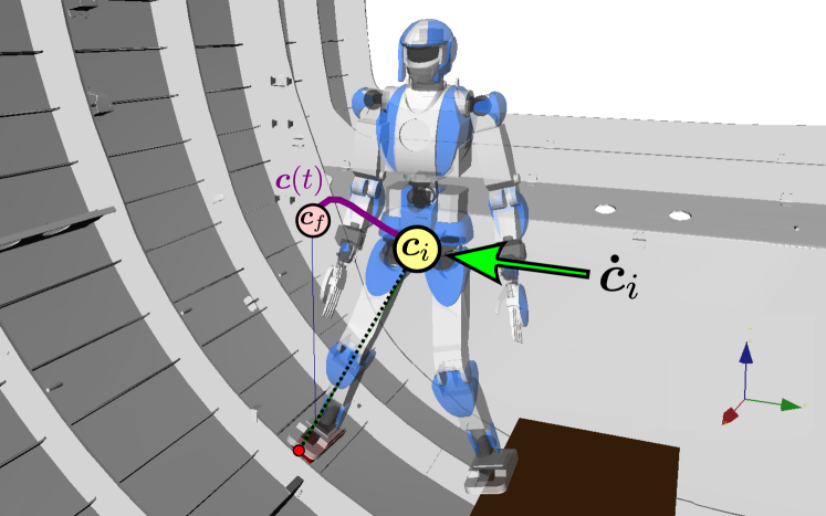
Figure 3: 3D balance control using both CoP and CoM height variations. The robot recovers from an undesired lateral push by stepping onto the fuselage of an A350 aircraft under construction. An initial velocity of 1.4 m s^-1 is absorbed in 1.5 s using both the ankle strategy and a 10 cm CoM height variation.

VI Concluding note

We saw how the boundedness condition can lead to an alternative optimization for 3D control of the inverted pendulum model. See [21] for an extension of this approach to 3D bipedal walking, addressing follow-up questions such as contact switches and the efficient resolution of the underlying numerical optimization.

-A Convexity of Equation (30)

Let us first consider the function $g(x,y)=\frac{1}{\sqrt{x}+\sqrt{y}}$. The trace and determinant of its Hessian $\nabla^{2}g$ are:

$$\mathrm{tr}(\nabla^{2}g) =\frac{x^{2}+3(x+y)\sqrt{xy}+y^{2}}{4(xy)^{3/2}(\sqrt{x}+\sqrt{y})^{3}}$$ (49)

$$\det(\nabla^{2}g) =\frac{3}{16(xy)^{3/2}(\sqrt{x}+\sqrt{y})^{4}}$$ (50)

Both are strictly positive quantities over the domain $x,y>0$, therefore $\nabla^{2}g$ is positive definite and $g$ is convex. Consider now the function $G(\bm{\varphi})$ defined by Equation (30) over the vector $\bm{\varphi}$ of positive values $\varphi_{1},\ldots,\varphi_{N}$: $G(\bm{\varphi})=\sum_{j=0}^{N-1}\Delta_{j}g(\varphi_{j+1},\varphi_{j})$. For any $t\in[0,1]$, $G(t\bm{\varphi}+(1-t)\bm{\varphi}^{\prime})$

$$=\sum_{j=0}^{N-1}\Delta_{j}g(t\varphi_{j+1}+(1-t)\varphi^{\prime}_{j+1},t\varphi_{j}+(1-t)\varphi^{\prime}_{j})$$

$$\leq\sum_{j=0}^{N-1}\Delta_{j}\left[tg(\varphi_{j+1},\varphi_{j})+(1-t)g(\varphi^{\prime}_{j+1},\varphi^{\prime}_{j})\right]$$ (51)

$$=tG(\bm{\varphi})+(1-t)G(\bm{\varphi}^{\prime})$$ (52)

Which establishes that $G$ is convex. ∎

-B Computing time trajectories

The piecewise constant values of $\lambda(s)$ are directly given by $\lambda_{j}=(\varphi_{j+1}-\varphi_{j})/\Delta_{j}$. Computing the time trajectory $\lambda(t)$ is then equivalent to finding the switch times $t_{j}$ such that $s(t_{j})=s_{j}$. Solving the equation of motion (1) of the IPM with constant $\lambda$, one can establish the recurrence relation:

$$t_{j}=t_{j+1}+\frac{1}{\sqrt{\lambda_{j}}}\log\left(\frac{\sqrt{\varphi_{j+1}}+\sqrt{\lambda_{j}}s_{j+1}}{\sqrt{\varphi_{j}}+\sqrt{\lambda_{j}}s_{j}}\right)$$ (53)

The same relation can be applied to find the map $s(t)$, giving $\omega(t)=\omega(s(t))=[\varphi_{j}+\lambda_{j}(s(t)^{2}-s_{j}^{2})]^{1/2}s(t)^{-1}$ for $t\in[t_{j},t_{j+1}]$ by Equation (26). Alternatively, one can solve the differential equation (3) from $t_{j}$ to get directly:

$$\omega(t)=\sqrt{\lambda_{j}}\frac{1-\upsilon_{j}\tanh(\sqrt{\lambda_{j}}(t-t_{j}))}{\upsilon_{j}-\tanh(\sqrt{\lambda_{j}}(t-t_{j}))}$$ (54)

where $\upsilon_{j}=\lambda_{j}/\omega(s_{j})=\lambda_{j}s_{j}/\varphi_{j}$.

References

- [1] S. Kajita, F. Kanehiro, K. Kaneko, K. Yokoi, and H. Hirukawa, “The 3d linear inverted pendulum mode: A simple modeling for a biped walking pattern generation,” in IEEE/RSJ International Conference on Intelligent Robots and Systems, vol. 1, 2001.
- [2] J. Pratt, J. Carff, S. Drakunov, and A. Goswami, “Capture point: A step toward humanoid push recovery,” in IEEE-RAS International Conference on Humanoid Robots, 2006.
- [3] T. Sugihara, “Standing stabilizability and stepping maneuver in planar bipedalism based on the best com-zmp regulator,” in IEEE-RAS International Conference on Robotics and Automation, 2009.
- [4] M. Morisawa, S. Kajita, F. Kanehiro, K. Kaneko, K. Miura, and K. Yokoi, “Balance control based on capture point error compensation for biped walking on uneven terrain,” in IEEE-RAS International Conference on Humanoid Robots, 2012.
- [5] J. Englsberger, C. Ott, and A. Albu-Schäffer, “Three-dimensional bipedal walking control based on divergent component of motion,” IEEE Transactions on Robotics, vol. 31, no. 2, 2015.
- [6] O. E. Ramos and K. Hauser, “Generalizations of the capture point to nonlinear center of mass paths and uneven terrain,” in IEEE-RAS International Conference on Humanoid Robots, 2015.
- [7] T. Koolen, M. Posa, and R. Tedrake, “Balance control using center of mass height variation: Limitations imposed by unilateral contact,” in IEEE-RAS International Conference on Humanoid Robots, 2016.
- [8] W. Gao, Z. Jia, and C. Fu, “Increase the feasible step region of biped robots through active vertical flexion and extension motions,” Robotica, vol. 35, no. 7, 2017.
- [9] J. E. Pratt and S. V. Drakunov, “Derivation and application of a conserved orbital energy for the inverted pendulum bipedal walking model,” in IEEE-RAS Int. Conf. on Robotics and Automation, 2007.
- [10] M. A. Hopkins, D. W. Hong, and A. Leonessa, “Humanoid locomotion on uneven terrain using the time-varying divergent component of motion,” in IEEE-RAS International Conf. on Humanoid Robots, 2014.
- [11] L. Lanari, S. Hutchinson, and L. Marchionni, “Boundedness issues in planning of locomotion trajectories for biped robots,” in Humanoid Robots, IEEE-RAS International Conference on, 2014.
- [12] L. Lanari and S. Hutchinson, “Inversion-based gait generation for humanoid robots,” in IEEE/RSJ International Conference on Intelligent Robots and Systems, 2015.
- [13] T. Takenaka, T. Matsumoto, and T. Yoshiike, “Real time motion generation and control for biped robot-1st report: Walking gait pattern generation,” in IEEE/RSJ Int. Conf. on Int. Robots and Systems, 2009.
- [14] P.-B. Wieber, R. Tedrake, and S. Kuindersma, “Modeling and control of legged robots,” in Springer Handbook of Robotics. Springer, 2016.
- [15] S. Kajita, M. Benallegue, R. Cisneros, T. Sakaguchi, S. Nakaoka, M. Morisawa, K. Kaneko, and F. Kanehiro, “Biped walking pattern generation based on spatially quantized dynamics,” in IEEE-RAS International Conference on Humanoid Robots, Nov. 2017.
- [16] S. Caron and A. Kheddar, “Multi-contact walking pattern generation based on model preview control of 3d com accelerations,” in IEEE-RAS International Conference on Humanoid Robots, 2016.
- [17] J. Carpentier, S. Tonneau, M. Naveau, O. Stasse, and N. Mansard, “A versatile and efficient pattern generator for generalized legged locomotion,” in IEEE Int. Conf. on Robotics and Automation, 2016.
- [18] S. Caron and A. Kheddar, “Dynamic walking over rough terrains by nonlinear predictive control of the floating-base inverted pendulum,” in IEEE/RSJ Int. Conf. on Intelligent Robots and Systems, 2017.
- [19] B. Ponton, A. Herzog, S. Schaal, and L. Righetti, “A convex model of humanoid momentum dynamics for multi-contact motion generation,” in IEEE-RAS International Conference on Humanoid Robots, 2016.
- [20] A. Pajon, S. Caron, G. De Magistris, S. Miossec, and A. Kheddar, “Walking on Gravel with Soft Soles using Linear Inverted Pendulum Tracking and Reaction Force Distribution,” in IEEE-RAS International Conference on Humanoid Robots, 2017.
- [21] S. Caron, A. Escande, L. Lanari, and B. Mallein, “Capturability-based analysis, optimization and control of 3d bipedal walking,” 2018, submitted.