varbvs: Fast Variable Selection for Large-scale Regression

4 Example: mapping a complex trait in outbred mice

In our second example, we illustrate the features of varbvs for genome-wide mapping of a complex trait. The data, downloaded from Zenodo (Carbonetto, 2017), are body and testis weight measurements recorded for 993 outbred mice, and genotypes at 79,748 single nucleotide polymorphisms (SNPs) for the same mice (Parker et al., 2016). Our main aim is to identify genetic variants contributing to variation in testis weight. The genotype data are represented in R as a $993\times 79,748$ matrix, geno. The phenotype data—body and testis weight, in grams—are stored in the "sacwt" and "testis" columns of the pheno matrix:

R> head(pheno[, c("sacwt", "testis")]) sacwt testis 26305 46.6 0.1396 26306 35.7 0.1692 26307 34.1 0.1878 26308 41.8 0.2002 26309 39.5 0.1875 26310 36.0 0.1826

The “cfw” vignette in the R package reproduces all the results of this analysis except for Fig. 4, which can be reproduced by running script cfw.cv.R accompanying this paper.

The standard approach in genome-wide mapping is to quantify support for a quantitative trait locus (QTL) separately at each SNP. For example, this was the approach taken in Parker et al. (2016). Here, we implement this univariate regression (“single-marker”) mapping approach using the -lm 2 option in GEMMA version 0.96 (Zhou and Stephens, 2012), which returns a likelihood-ratio test p value for each SNP. We compare this single-marker analysis against a varbvs multiple regression (“multi-marker”) analysis of the same data.

In the varbvs analysis, the quantitative trait (testis weight) is modeled as a linear combination of the covariate (body weight) and the candidate variables (the 79,748 SNPs). As before, the model fitting is accomplished with a single function call:

R> fit <- varbvs(geno, as.matrix(pheno[, "sacwt"]), pheno[, "testis"], + sa = 0.05, logodds = seq(-5, -3, 0.25))

This call is completed in less than 4 minutes on a MacBook Air with a 1.86 GHz Intel CPU, 4 GB of memory and R 3.3.3. Note that, to simplify this example, we have fixed sa to 0.05, a choice informed by our power calculations. In this application, it would be preferable to average over a range of settings to avoid sensitivity to prior choice.

Once the model fitting is completed, we quickly generate a summary of the results using the summary function:

R> print(summary(fit)) Summary of fitted Bayesian variable selection model: family: gaussian num. hyperparameter settings: 9 samples: 993 iid variable selection prior: yes variables: 79748 fit prior var. of coefs (sa): no covariates: 2 fit residual var. (sigma): yes maximum log-likelihood lower bound: 2428.7093 proportion of variance explained: 0.149 [0.090,0.200] Hyperparameters: estimate Pr>0.95 candidate values sigma 0.000389 [0.000379,0.000404] NA–NA sa NA [NA,NA] 0.05–0.05 logodds -3.78 [-4.25,-3.50] (-5.00)–(-3.00) Selected variables by probability cutoff: >0.10 >0.25 >0.50 >0.75 >0.90 >0.95 3 3 3 2 2 1 Top 5 variables by inclusion probability: index variable prob PVE coef Pr(coef.>0.95) rs6279141 59249 rs6279141 1.0000 0.0631 -0.00806 [-0.010,-0.007] rs33217671 24952 rs33217671 0.9351 0.0220 0.00509 [+0.003,+0.007] rs33199318 9203 rs33199318 0.6869 0.0170 0.00666 [+0.004,+0.009] rs52004293 67415 rs52004293 0.0739 0.0136 0.00347 [+0.002,+0.005] rs253722776 44315 rs253722776 0.0707 0.0133 -0.00369 [-0.005,-0.002]

This summary tells us that only 3 out of the 79,748 SNPs are included in the model with posterior probability greater than 0.5, and that the included SNPs explain 15% of the variance of testis weight. (Precisely, this is the variance explained in testis weight residuals after controlling for body weight.) Further, a single SNP (rs6279141) accounts for over 6% of variance in testis weight. This SNP is located on chromosome 13 approximately 1 Mb from Inhba, a gene that has been previously shown to affect testis morphogenesis (Mendis et al., 2011; Mithraprabhu et al., 2010; Tomaszewski et al., 2007).

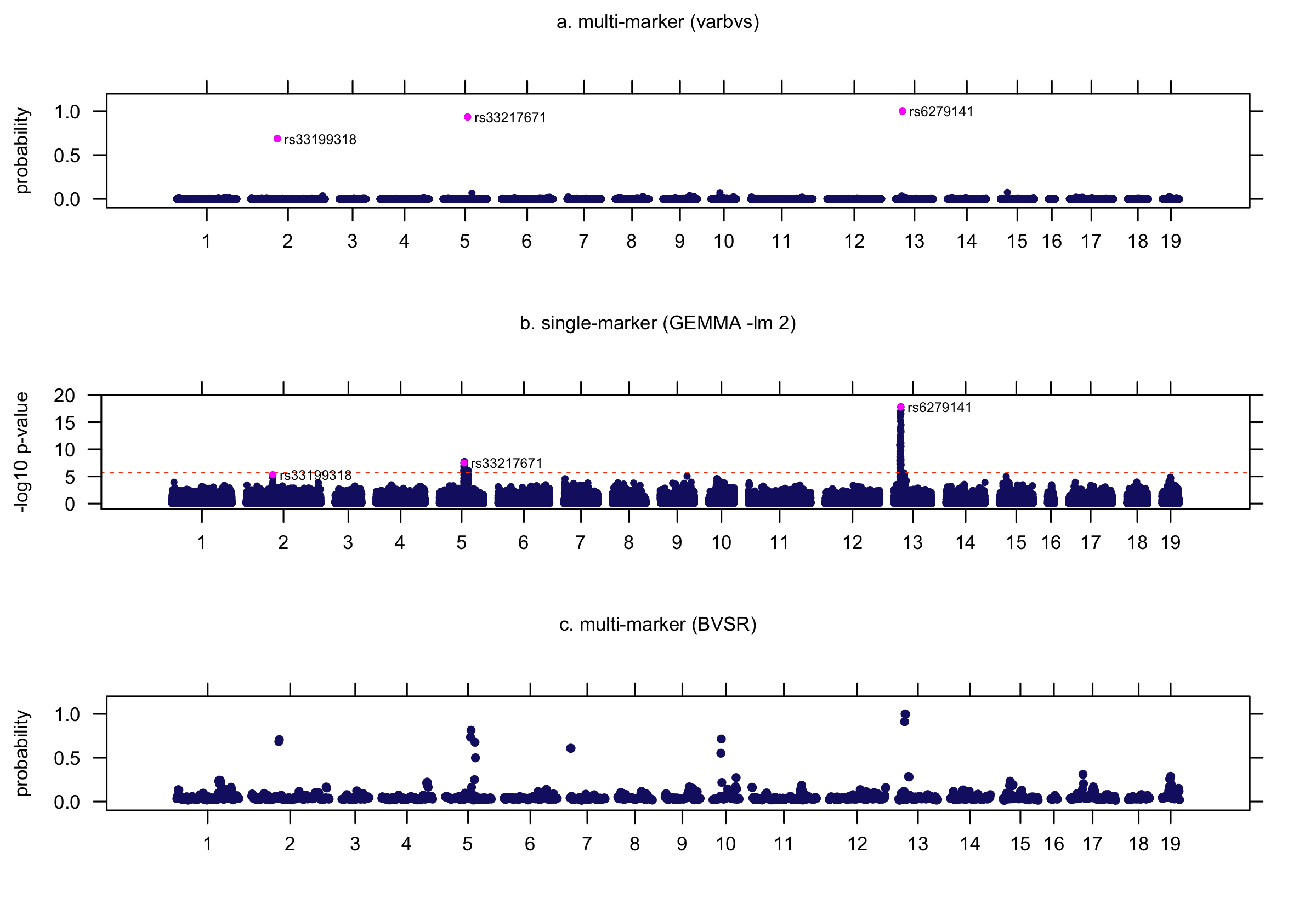
Figure 3: QTL mapping of a complex trait in outbred mice. (a) Posterior inclusion probabilities for all 79,748 candidate SNPs on chromosomes 1–19 computed using varbvs. SNPs with PIPs greater than 0.5 are highlighted. (b) p values for the same candidate SNPs computed using GEMMA. threshold determined via permutation analysis, at $\mbox{{\em p}~{}value}=2\times 10^{-6}$ (Parker et al., 2016). (c) Posterior probabilities computed using the BVSR method in GEMMA version 0.96 (Zhou et al., 2013). In BVSR, since multiple correlated SNPs at a single QTL are expected to be included in the model with lower probability, plotting individual PIPs does not highlight the QTLs. Therefore, the results are summarized by dividing each chromosome into contiguous segments containing 100 SNPs, in which consecutive segments overlap by 50 SNPs, and computing the posterior probability that at least 1 SNP is included within each of these segments.

We can also quickly create a visual summary of the results using the plot function:

R> print(plot(fit, vars = c("rs33199318", "rs33217671", "rs6279141"), + groups = map$chr,gap=1500))\par TheoutputisshowninFig.~{}\ref{fig:cfw}a.Notethatthe\code{plot}functionhasa\code{"group"}argument,whichallowsustoarrangethevariableselectionresultsbychromosome.\par\par Itisinformativetocomparetheseprobabilitiesagainstthe``single-marker^{\prime\prime}{\em p}~{}valuesthatignorecorrelationsbetweenSNPs(Fig.~{}\ref{fig:cfw}b).Reassuringly,thelociwiththestrongestsupportforassociationinthesingle-markeranalysis(Fig.~{}\ref{fig:cfw}b)alsoexhibitthestrongestsupportforassociationinthemulti-markeranalysis(Fig.~{}\ref{fig:cfw}a).Further,SNPsincludedwiththehighestposteriorprobabilitiesareamongtheSNPswiththesmallest{\em p}~{}values.OneQTLonchromosome2isnotsignificantinthesingle-markeranalysis($p value = 5.2 ×10^-6$),yetshowsmoderateprobabilityofassociationinthemulti-markeranalysis.Themulti-markerassociationsignalatthislocusisconcentratedinasmallregionthatcontainsasinglegene,{\sf\em Myo3b},providinganadditionaltestisweightgeneforfurtherinvestigation.\par InFig.~{}\ref{fig:cfw}b,weobservethatmanySNPshavelow{\em p}~{}valuesateachoftheidentifiedtestisweightloci.ThisillustratesthecommonsituationinGWASinwhichmanySNPsatasinglelocusareassociatedwiththetrait.Ingeneral,whenmultiplevariablesarestronglycorrelatedwitheachother,thefully-factorizedvariationalapproximationin\pkg{varbvs}tendstoconcentratetheposteriormassonasinglevariable.\par\begin{figure}[t!]\begin{center}\includegraphics[width=252.94499pt,keepaspectratio={true}]{cfwcv.pdf}\end{center}\@@toccaption{{\lx@tag[ ]{{4}}{Scatterplotcomparingaccuracyof\pkg{varbvs}andBVSRpredictions.Toassesspredictionaccuracy,weperformasimplecross-validationexperimentinwhichthemousedataaresplitevenlyinto10testdatasets:ineachofthe10roundsofcross-validation,the\pkg{varbvs}andBVSRmodelsarefittotheremainingtrainingsamples,thenthepredictionsareevaluatedinthetestset.The$x$and$y$axesintheplotshowdifferencesbetweenpredictedandobservedphenotype(testisweightcontrollingforbodyweight)intheleft-outtestsamples.Thesedifferencesarenormalizedbythestandarddeviationofthephenotypecomputedfromthefullsample.Theadjoiningscript\code{cfw.cv.R}reproducestheresultsofthecross-validationexperiment,aswellasthisfigure.TheBVSRmethodisimplementedinGEMMAversion0.96.}}}\@@caption{{\lx@tag[: ]{{Figure 4}}{Scatterplotcomparingaccuracyof\pkg{varbvs}andBVSRpredictions.Toassesspredictionaccuracy,weperformasimplecross-validationexperimentinwhichthemousedataaresplitevenlyinto10testdatasets:ineachofthe10roundsofcross-validation,the\pkg{varbvs}andBVSRmodelsarefittotheremainingtrainingsamples,thenthepredictionsareevaluatedinthetestset.The$x$and$y$axesintheplotshowdifferencesbetweenpredictedandobservedphenotype(testisweightcontrollingforbodyweight)intheleft-outtestsamples.Thesedifferencesarenormalizedbythestandarddeviationofthephenotypecomputedfromthefullsample.Theadjoiningscript\code{cfw.cv.R}reproducestheresultsofthecross-validationexperiment,aswellasthisfigure.TheBVSRmethodisimplementedinGEMMAversion0.96.}}}\end{figure}\par Wealsoassessedtheaccuracyofthevariationalapproximationbycomparingthe\pkg{varbvs}results(Fig.~{}\ref{fig:cfw}a)againstanothermethod,BVSR\cite[citep]{(\@@bibref{AuthorsPhrase1Year}{zhou-2013}{\@@citephrase{, }}{})},thatusesaverysimilarmodel.TheBVSRmethodimplementedinGEMMAusesMCMCtoestimateposteriorprobabilities.ComparingpanelsaandcinFig.~{}\ref{fig:cfw},BVSRyieldsamorecomplexmodelinwhichhundredsofSNPsareincludedinthemodelwithlowprobability---yetthelociwiththestrongestsupportinthe\pkg{varbvs}andBVSRanalysescloselyagree.Thesimpler\pkg{varbvs}modelalsoachievessimilarpredictionaccuracytotheBVSRmodel;inasimplecross-validationexperimentinwhich10\%ofthesamplesineachroundareusedtotestthemodel,thepredictionerrorsofthe\pkg{varbvs}andBVSRmethodsare97\%correlated(Fig.~{}\ref{fig:cfw-cv}).\par\par$

5 Example: mapping Crohn’s disease risk loci

Our third example again illustrates varbvs’s ability to tackle large data sets for mapping genetic loci contributing to a complex trait. The data set in this example contains 4,686 samples (1,748 Crohn’s disease cases, 2,938 controls) and 442,001 SNPs (Wellcome Trust Case Control Consortium, 2007). The genotypes are stored in a $4,686\times 442,001$ matrix X, and the binary outcome is disease status (0 = control, 1 = case): > print(summary(factor(y))) 0 1 2938 1748 We model Crohn’s disease disease status using logistic regression, with the 442,001 SNPs as candidate variables, and no additional covariates. On a machine with a 2.5 GHz Intel Xeon CPU, fitting the BVS model to the data took 39 hours to complete: R> fit <- varbvs(X, NULL, y, family = "binomial", logodds = seq(-6,-3,0.25), n0 = 0) The “cd” vignette reproduces all the results and plots shown here. Since the data needed to run the script cannot be made publicly available due to data sharing restrictions, those wishing to reproduce this analysis must apply for data access by contacting the Wellcome Trust Case Control Consortium.

Similar to the previous examples, the fitted regression model is very sparse; only 8 out of the 442,001 candidate variables are included in the model with probability at least 0.5: R> print(summary(fit,nv = 9)) Summary of fitted Bayesian variable selection model: family: binomial num. hyperparameter settings: 13 samples: 4686 iid variable selection prior: yes variables: 442001 fit prior var. of coefs (sa): yes fit approx. factors (eta): yes maximum log-likelihood lower bound: -3043.2388 Hyperparameters: estimate Pr>0.95 candidate values sa 0.032 [0.0201,0.04] NA–NA logodds -4.06 [-4.25,-3.75] (-6.00)–(-3.00) Selected variables by probability cutoff: >0.10 >0.25 >0.50 >0.75 >0.90 >0.95 13 10 8 7 7 7 Top 9 variables by inclusion probability: index variable prob PVE coef* Pr(coef.>0.95) 1 71850 rs10210302 1.000 NA -0.313 [-0.397,-0.236] 2 10067 rs11805303 1.000 NA 0.291 [+0.207,+0.377] 3 140044 rs17234657 1.000 NA 0.370 [+0.255,+0.484] 4 381590 rs17221417 1.000 NA 0.279 [+0.192,+0.371] 5 402183 rs2542151 0.992 NA 0.290 [+0.186,+0.392] 6 271787 rs10995271 0.987 NA 0.236 [+0.151,+0.323] 7 278438 rs7095491 0.969 NA 0.222 [+0.141,+0.303] 8 168677 rs9469220 0.586 NA -0.194 [-0.269,-0.118] 9 22989 rs12035082 0.485 NA 0.195 [+0.111,+0.277] *See help(varbvs) about interpreting coefficients in logistic regression.

The varbvs results, summarized in Fig. 5a, provide strong support for nearly the same reported p values at the previously used “whole-genome” significance threshold, $5\times 10^{-7}$; in particular, the 7 SNPs included in the regression model with probability greater than 0.9 correspond to the smallest trend p values, between $7.1\times 10^{-14}$ and $2.68\times 10^{-7}$ (Wellcome Trust Case Control Consortium, 2007). Additionally, the SNP the highest posterior probability is most cases the exact same SNP with the smallest trend p value. (See Carbonetto and Stephens 2013 for an extended comparison of the p values and PIPs.) Only one disease locus, near gene IRGM on chromosome 5, has substantially stronger support in the single-marker analysis; the originally reported p value is $5.1\times 10^{-8}$, whereas the varbvs analysis yields a largest posterior probability of $0.05$ at this locus.

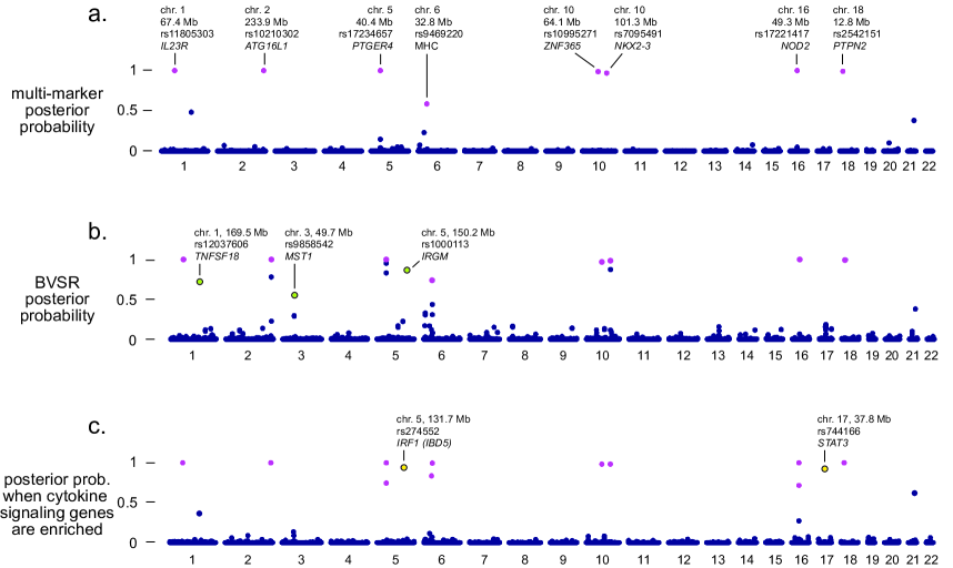
Figure 5: varbvs and BVSR analysis of Crohn’s disease data. (a) Posterior inclusion probabilities for all 442,001 candidate SNPs on chromosomes 1–22. SNPs with PIP greater than 0.5 are highlighted. Human Genome Assembly hg17 (NCBI release 35). (b) Posterior probabilities estimated in BVSR (Zhou et al., 2013). Similar to the mouse data, each chromosome is divided into overlapping 50-SNP segments, and the plot shows the posterior probability that at least 1 SNP is included within each segment. Three points are highlighted in light green; these are segments with posterior probability greater than 0.5 in the BVSR analysis that do not contain a SNP with PIP greater than 0.5 in the varbvs analysis. (c) PIPs for all SNPs conditioned on enrichment of cytokine signaling genes. Two SNPs are highlights in yellow; they are the two SNPs with a PIP greater than 0.5 only after prioritizing SNPs near cytokine signaling genes.

To further validate the varbvs analysis of the Crohn’s disease data, we compared the varbvs results against posterior probabilities computed using the BVSR method. As before, we obtain similar variable selection results; the loci with the strongest support in the varbvs analysis (Fig. 5a) are the same loci identified by the BVSR method (Fig. 5b) aside from a few loci with moderate support in the BVSR analysis near genes TNFSF18, MST1 and IRGM.

6 Example: gene set enrichment analysis in Crohn’s disease

In this section, we revisit the Crohn’s disease data set to demonstrate the use of varbvs for model comparison. This analysis is implemented in the “cytokine” vignette.

Here, we incorporate additional information about the 442,001 candidate variables, stored in a vector, cytokine: R> data(cytokine) R> print(summary(factor(cytokine))) 0 1 435290 6711

An entry of 1 means that the SNP is located within 100 kb of a gene in the “Cytokine signaling in immune system” gene set. This gene set was previously identified in an interrogation of 3,158 gene sets from 8 publicly available biological pathway databases (Carbonetto and Stephens, 2013).

To assess relevance of cytokine signaling genes to Crohn’s disease risk, we modify the prior so that SNPs near cytokine signaling genes are included in the model with higher probability (i.e., cytokine signaling genes are “enriched” for Crohn’s disease risk loci). To simplify this example, the default prior log-odds is set to -4, which is the maximum-likelihood value from the above analysis. We evaluate 13 settings of the modified prior, ranging from -4 (1 out of 10,000 SNPs is included in the model) to -1 (approximately 1 out of 10 SNPs is included): R> logodds <- matrix(-4,442001,13) R> logodds[cytokine == 1,] <- matrix(seq(0,3,0.25) - 4,6711,13,byrow = TRUE) We then fit the BVS model to the data using this modified prior: R> fit.cytokine <- varbvs(X, NULL, y, family = "binomial", logodds = logodds, n0 = 0)

The new variable selection results are summarized in Fig. 5c. The SNPs identified in the previous analysis are retained under the new prior. Further, 2 new SNPs, near genes IRF1 and STAT3, show strong support for association only after allowing for enrichment of associations near cytokine signaling genes.

To assess support for this model, we compute a Bayes factor (Kass and Raftery, 1995) that compares against the “null” model in which all SNPs are equally likely to be included a priori (i.e., an exchangeable prior):

R> fit.null <- varbvs(X, NULL, y, "binomial", logodds = -4, n0 = 0) R> BF <- varbvsbf(fit.null, fit.cytokine) R> print(format(, scientific = TRUE)) [1] "9.355e+05" This Bayes factor is strong evidence that Crohn’s disease risk loci are found with greater frequency near cytokine signaling genes.

7 Summary and discussion

In this paper, we illustrated the benefits of Bayesian variable selection techniques for regression analysis, and showed that varbvs provides a user-friendly interface for applying BVS to large data sets. Mathematical details and derivations of the algorithms are found in the Appendix and in Carbonetto and Stephens (2012). In the remainder, we provide some additional background and guidance.

As our examples illustrate, one benefit of BVS is that it provides a measure of uncertainty in the parameter estimates. Assessing uncertainty is often not done in practice because it requires careful selection of priors. Therefore, we have provided default priors that are suitable in many settings. This allows the practitioner to expedite the analysis, and perhaps revisit the prior choices at a later date. The default priors are based on detailed discussions from our earlier work (Guan and Stephens, 2011; Servin and Stephens, 2007; Zhou et al., 2013). As an alternative, varbvs also allows for computation of hyperparameter point estimates.

Fast computation of posterior probabilities is made possible by the formulation of a variational approximation derived from a simple conditional independence assumption. Even when many of the variables are strongly correlated, this approximation can often yield accurate inferences so long as individual posterior statistics are interpreted carefully. The computational complexity of the co-ordinate ascent algorithm for fitting the variational approximation is linear in the number of samples and in the number of variables so long as the correlations between variables are mostly small. This makes the algorithm suitable for many genetic data sets since correlations are limited by recombination. However, for data sets with widespread correlations between variables, convergence of the algorithm can be slow. We are currently investigating faster alternatives using quasi-Newton methods and acceleration schemes such as SQUAREM (Varadhan and Roland, 2008; Varadhan, 2016).

In practice, final estimates can be sensitive to initialization of the variational parameters. We have reduced this sensitivity by including an additional optimization step that first identifies a good initialization of the variational parameters (Sec. LABEL:sec:posterior-hyperparameters). However, it is good practice to verify that different random initializations of these parameters do not yield substantially different conclusions. The documentation for function varbvs gives further guidance on this, as well as guidelines for correctly interpreting variational estimates of the posterior statistics.

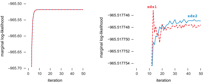
Figure 6: Convergence of varbvs model fitting algorithm with less numerically stable (xdx1) and more numerically stable (xdx2) updates. The vertical axes show the variational lower bound to the marginal log-likelihood, which is also the objective function being maximized; the co-ordinate ascent updates terminate when they no longer increase the lower bound. The right-hand plot is a magnified version of the left-hand plot.

Finally, we would like to remark on an often overlooked aspect of statistical analyses—numerical stability. In the logistic regression model, part of the variational optimization algorithm involves computing the diagonal entries of the matrix product ${\bf X}^{T}\hat{D}{\bf X}$, in which $\hat{D}$ is an $n\times n$ diagonal matrix (see the Appendix). In the MATLAB implementation, the following two lines of code are mathematically equivalent, xdx1 = diag(X’*D*X) - (X’*d).^2/sum(d) xdx2 = diag(X’*D*X) - (X’*(d/sqrt(sum(d)))).^2 where d = diag(D). Yet, in floating-point arithmetic, the order of operations affects the numerical precision of the final result, which can in turn affect the stability of the co-ordinate ascent updates. To illustrate this, we applied varbvs, using the two different updates (xdx1 and xdx2), to a data set with simulated variables and a binary outcome. In Fig. 6, we see that the second update (xdx2), corresponding to the solid blue line in the plots, produced iterates that progressed more smoothly to a stationary point of the objective function, whereas the first update (xdx1) terminated prematurely because it produced a large decrease in the objective. This illustrates the more general point that numerical stability of operations can impact the quality of the final solution, particularly for large data sets.

Appendix A About this document

This manuscript was prepared using the Sweave function from the weaver package (Falcon, 2017). The code chunk below records the version of R and the packages that were used to generate the results contained in this manuscript.

R> sessionInfo() R version 3.4.1 (2017-06-30) Platform: x86_64-apple-darwin15.6.0 (64-bit) Running under: macOS Sierra 10.12.6

Matrix products: default BLAS: /Library/Frameworks/R.framework/Versions/3.4/Resources/lib/libRblas.0.dylib LAPACK: /Library/Frameworks/R.framework/Versions/3.4/Resources/lib/libRlapack.dylib

locale: [1] en_US.UTF-8/en

References

- Blei et al. (2016) Blei DM, Kucukelbir A, McAuliffe JD (2016). “Variational Inference: A Review for Statisticians.” arXiv:1601.00670v3.
- Bottolo and Richardson (2010) Bottolo L, Richardson S (2010). “Evolutionary Stochastic Search for Bayesian Model Exploration.” Bayesian Analysis, 5(3), 583–618.
- Breheny and Huang (2011) Breheny P, Huang J (2011). “Coordinate Descent Algorithms for Nonconvex Penalized Regression, with Applications to Biological Feature Selection.” Annals of Applied Statistics, 5(1), 232–253.
- Carbonetto (2017) Carbonetto P (2017). “Physiological Trait and Genotype Data for 1,038 Outbred CFW Mice.” 10.5281/zenodo.546142. URL https://doi.org/10.5281/zenodo.546142.
- Carbonetto and Stephens (2012) Carbonetto P, Stephens M (2012). “Scalable Variational Inference for Bayesian Variable Selection in Regression, and Its Accuracy in Genetic Association Studies.” Bayesian Analysis, 7(1), 73–108.
- Carbonetto and Stephens (2013) Carbonetto P, Stephens M (2013). “Integrated Enrichment Analysis of Variants and Pathways in Genome-wide Association Studies Indicates Central Role for IL-2 Signaling Genes in Type 1 Diabetes, and Cytokine Signaling Genes in Crohn’s Disease.” PLoS Genetics, 9(10), e1003770.
- Chipman et al. (2001) Chipman H, George EI, McCulloch RE (2001). “The Practical Implementation of Bayesian Model Selection.” In Model Selection, volume 38 of IMS Lecture Notes, pp. 65–116.
- Clyde et al. (2011) Clyde MA, Ghosh J, Littman ML (2011). “Bayesian Adaptive Sampling for Variable Selection and Model Averaging.” Journal of Computational and Graphical Statistics, 20(1), 80–101.
- Dellaportas et al. (2002) Dellaportas P, Forster JJ, Ntzoufras I (2002). “On Bayesian Model and Variable Selection Using MCMC.” Statistics and Computing, 12(1), 27–36.
- Dettling (2004) Dettling M (2004). “BagBoosting for Tumor Classification with Gene Expression Data.” Bioinformatics, 20(18), 3583–3593.
- Erbe et al. (2012) Erbe M, Hayes BJ, Matukumalli LK, Goswami S, Bowman PJ, Reich CM, Mason BA, Goddard ME (2012). “Improving Accuracy of Genomic Predictions Within and Between Dairy Cattle breeds with Imputed High-density Single Nucleotide Polymorphism Panels.” Journal of Dairy Science, 95(7), 4114–4129.
- Falcon (2017) Falcon S (2017). weaver: Tools and Extensions for Processing Sweave Documents. URL https://dx.doi.org/doi:10.18129/B9.bioc.weaver.
- Friedman et al. (2007) Friedman J, Hastie T, Höfling H, Tibshirani R (2007). “Pathwise Coordinate Optimization.” Annals of Applied Statistics, 2, 302–332.
- Friedman et al. (2010) Friedman J, Hastie T, Tibshirani R (2010). “Regularization Paths for Generalized Linear Models via Coordinate Descent.” Journal of Statistical Software, 33(1), 1–22. URL http://www.jstatsoft.org/v033/i01.
- George (2000) George EI (2000). “The Variable Selection Problem.” Journal of the American Statistical Association, 95(452), 1304–1308.
- George and McCulloch (1993) George EI, McCulloch RE (1993). “Variable Selection via Gibbs Sampling.” Journal of the American Statistical Association, 88(423), 881–889.
- Golub et al. (1999) Golub TR, Slonim DK, Tamayo P, Huard C, Gaasenbeek M, Mesirov JP, Coller H, Loh ML, Downing JR, Caligiuri MA, Bloomfield CD, Lander ES (1999). “Molecular Classification of Cancer: Class Discovery and Class Prediction by Gene Expression Monitoring.” Science, 286(5439), 531–537.
- Guan and Stephens (2011) Guan Y, Stephens M (2011). “Bayesian Variable Selection Regression for Genome-wide Association Studies, and Other Large-scale Problems.” Annals of Applied Statistics, 5(3), 1780–1815.
- Heskes et al. (2004) Heskes T, Zoeter O, Wiegerinck W (2004). “Approximate Expectation Maximization.” In S Thrun, LK Saul, B Schölkopf (eds.), Advances in Neural Information Processing Systems 16, pp. 353–360.
- Hoeting et al. (1999) Hoeting JA, Madigan D, Raftery AE, Volinsky CT (1999). “Bayesian Model Averaging: A Tutorial.” Statistical Science, 14(4), 382–401.
- Hoggart et al. (2008) Hoggart CJ, Whittaker JC, De Iorio M, Balding DJ (2008). “Simultaneous Analysis of All SNPs in Genome-wide and Re-sequencing Association Studies.” PLoS Genetics, 7(4), e1000130.
- Jaakkola and Jordan (2000) Jaakkola TS, Jordan MI (2000). “Bayesian Parameter Estimation via Variational Methods.” Statistics and Computing, 10(1), 25–37.
- Jefferys and Berger (1992) Jefferys WH, Berger JO (1992). “Ockham’s Razor and Bayesian analysis.” American Scientist, 80(1), 64–72.
- Jordan et al. (1999) Jordan MI, Ghahramani Z, Jaakkola TS, Saul LK (1999). “An Introduction to Variational Nethods for Graphical Models.” Machine Learning, 37(2), 183–233.
- Kass and Raftery (1995) Kass RE, Raftery AE (1995). “Bayes Factors.” Journal of the American Statistical Association, 90(430), 773–795.
- Lee et al. (2008) Lee SH, van der Werf JHJ, Hayes BJ, Goddard ME, Visscher PM (2008). “Predicting Unobserved Phenotypes for Complex Traits from Whole-genome SNP Data.” PLoS Genetics, 4, e1000231.
- Logsdon et al. (2010) Logsdon BA, Hoffman GE, Mezey JG (2010). “A Variational Bayes Algorithm for Fast and Accurate Multiple Locus Genome-wide Association Analysis.” BMC Bioinformatics, 11, 58.
- MacKay (1992) MacKay DJC (1992). “Bayesian Interpolation.” Neural Computation, 4(3), 415–447.
- Mendis et al. (2011) Mendis SHS, Meachem SJ, Sarraj MA, Loveland KL (2011). “Activin A Balances Sertoli and Germ Cell Proliferation in the Fetal Mouse Testis.” Biology of Reproduction, 84(2), 379–391.
- Meuwissen et al. (2001) Meuwissen THE, Hayes B, Goddard M (2001). “Prediction of Total Genetic Value Using Genome-wide Dense Marker Maps.” Genetics, 157(4), 1819–1829.
- Mitchell and Beauchamp (1988) Mitchell TJ, Beauchamp JJ (1988). “Bayesian Variable Selection in Linear Regression.” Journal of the American Statistical Association, 83(404), 1023–1032.
- Mithraprabhu et al. (2010) Mithraprabhu S, Mendis S, Meachem SJ, Tubino L, Matzuk MM, Brown CW, Loveland KL (2010). “Activin Bioactivity Affects Germ Cell Differentiation in the Postnatal Mouse Testis In Vivo.” Biology of Reproduction, 82(5), 980–990.
- Moser et al. (2015) Moser G, Lee SH, Hayes BJ, Goddard ME, Wray NR, Visscher PM (2015). “Simultaneous Discovery, Estimation and Prediction analysis of Complex Traits Using a Bayesian Mixture Model.” PLOS Genetics, 11(4), e1004969.
- Neal et al. (1998) Neal R, , Hinton G (1998). “A View of the EM Algorithm that Justifies Incremental, Sparse, and Other Variants.” In M Jordan (ed.), Learning in Graphical Models, pp. 355–368. Kluwer Academic Publishers, Dordrecht.
- O’Brien and Dunson (2004) O’Brien SM, Dunson DB (2004). “Bayesian Multivariate Logistic Regression.” Biometrics, 60(3), 739–746.
- O’Hara and Sillanpäa (2009) O’Hara RB, Sillanpäa MJ (2009). “A Review of Bayesian Variable Selection Methods: What, How and Which.” Bayesian Analysis, 4(1), 85–117.
- Ormerod and Wand (2010) Ormerod JT, Wand MP (2010). “Explaining Variational Approximations.” The American Statistician, 64(2), 140–153.
- Parker et al. (2016) Parker CC, Gopalakrishnan S, Carbonetto P, Gonzales NM, Leung E, Park YJ, Aryee E, Davis J, Blizard DA, Ackert-Bicknell CL, Lionikas A, Pritchard JK, Palmer AA (2016). “Genome-wide Association Study of Behavioral, Physiological and Gene Expression Traits in Outbred CFW Mice.” Nature Genetics, 48(8), 919–926.
- Perez and de los Campos (2014) Perez P, de los Campos G (2014). “Genome-Wide Regression and Prediction with the BGLR Statistical Package.” Genetics, 198(2), 483–495.
- \proglangR Core Team (2016) \proglangR Core Team (2016). R: A Language and Environment for Statistical Computing. R Foundation for Statistical Computing, Vienna, Austria. URL https://www.R-project.org.
- Servin and Stephens (2007) Servin B, Stephens M (2007). “Imputation-based Analysis of Association Studies: Candidate Regions and Quantitative Traits.” PLoS Genetics, 3(7), 1296–1308.
- The MathWorks, Inc. (2016) The MathWorks, Inc (2016). MATLAB: The Language of Technical Computing, Version R2016a. The MathWorks, Inc., Natick, Massachusetts. URL http://www.mathworks.com/products/matlab.
- Tibshirani (1994) Tibshirani R (1994). “Regression Selection and Shrinkage via the Lasso.” Journal of the Royal Statistical Society Series B, 58(1), 267–288.
- Tibshirani et al. (2005) Tibshirani R, Saunders M, Rosset S, Zhu J, Knight K (2005). “Sparsity and Smoothness via the Fused Lasso.” Journal of the Royal Statistical Society Series B, 67(1), 91–108.
- Tomaszewski et al. (2007) Tomaszewski J, Joseph A, Archambeault D, Yao HCH (2007). “Essential Roles of Inhibin Beta A in Mouse Epididymal Coiling.” Proceedings of the National Academy of Sciences, 104(27), 11322–11327.
- Varadhan (2016) Varadhan R (2016). SQUAREM: Squared Extrapolation Methods for Accelerating EM-Like Monotone Algorithms. URL http://CRAN.R-project.org/package=SQUAREM.
- Varadhan and Roland (2008) Varadhan R, Roland C (2008). “Simple and Globally Convergent Methods for Accelerating the Convergence of any EM Algorithm.” Scandinavian Journal of Statistics, 35(2), 335–353.
- Wainwright and Jordan (2008) Wainwright MJ, Jordan MI (2008). “Graphical Models, Exponential Families, and Variational Inference.” Foundations and Trends in Machine Learning, 1(1–2), 1–305.
- Wallace et al. (2015) Wallace C, Cutler AJ, Pontikos N, Pekalski ML, Burren OS, Cooper JD, García AR, Ferreira RC, Guo H, Walker NM, Smyth DJ, Rich SS, Onengut-Gumuscu S, Sawcer SJ, Ban M, Richardson S, Todd JA, Wicker LS (2015). “Dissection of a Complex Disease Susceptibility Region Using a Bayesian Stochastic Search Approach to Fine Mapping.” PLOS Genetics, 11(6), e1005272.
- Wellcome Trust Case Control Consortium (2007) Wellcome Trust Case Control Consortium (2007). “Genome-wide Association Study of 14,000 Cases of Seven Common Diseases and 3,000 Shared Controls.” Nature, 447(7145), 661–678.
- Zhou et al. (2013) Zhou X, Carbonetto P, Stephens M (2013). “Polygenic Modeling with Bayesian Sparse Linear Mixed Models.” PLoS Genetics, 9(2), e1003264.
- Zhou and Stephens (2012) Zhou X, Stephens M (2012). “Genome-wide Efficient Mixed-model Analysis for Association Studies.” Nature Genetics, 44(7), 821–824.
- Zou and Hastie (2005) Zou H, Hastie T (2005). “Regularization and Variable Selection via the Elastic Net.” Journal of the Royal Statistical Society Series B, 67(2), 301–320.