On Collaborative Compressive Sensing Systems:
The Framework, Design and Algorithm

Abstract

Based on the maximum likelihood estimation principle, we derive a collaborative estimation framework that fuses several different estimators and yields a better estimate. Applying it to compressive sensing (CS), we propose a collaborative CS (CCS) scheme consisting of a bank of $K$ CS systems that share the same sensing matrix but have different sparsifying dictionaries. This CCS system is expected to yield better performance than each individual CS system, while requiring the same time as that needed for each individual CS system when a parallel computing strategy is used. We then provide an approach to designing optimal CCS systems by utilizing a measure that involves both the sensing matrix and dictionaries and hence allows us to simultaneously optimize the sensing matrix and all the $K$ dictionaries. An alternating minimization-based algorithm is derived for solving the corresponding optimal design problem. With a rigorous convergence analysis, we show that the proposed algorithm is convergent. Experiments are carried out to confirm the theoretical results and show that the proposed CCS system yields significant improvements over the existing CS systems in terms of the signal recovery accuracy.

62H35, 68P30, 68U10, 94A08

1 Introduction

Compressive (or compressed) sensing (CS), aiming to sample signals beyond Shannon-Nyquist limit [16, 17, 19, 24], is a mathematical framework that efficiently compresses a signal vector $\bm{x}\in\Re^{N}$ by a measurement vector $\bm{y}\in\Re^{M}$ of the form

(1) $$\bm{y}=\bm{\Phi}\bm{x},$$

where $\bm{\Phi}\in\Re^{M\times N}$ ($M\ll N$) is a carefully chosen sensing matrix capturing the information contained in the signal vector $\bm{x}$.

As $M\ll N$, we have to exploit additional constraints or structures on the signal vector $\bm{x}$ in order to recover it from the measurement $\bm{y}$ and sparsity is such a structure. In CS, it is assumed that the original signal $\bm{x}$ can be expressed as a linear combination of few elements/atoms from a $l_{2}$-normalized set $\{\bm{\psi}_{\ell}\}$, i.e., $||\bm{\psi}_{\ell}||_{2}=1,\leavevmode\nobreak\ \forall\leavevmode\nobreak\ \ell$:

(2) $$\bm{x}=\sum_{\ell=1}^{L}\bm{\psi}_{\ell}s_{\ell}=\bm{\Psi}\bm{s},$$

where $\bm{\Psi}:=\begin{bmatrix}\bm{\psi}_{1}&\bm{\psi}_{2}&\cdots&\bm{\psi}_{L}\end{bmatrix}\in\Re^{N\times L}$ is called the dictionary and the entries of $\bm{s}\in\Re^{L}$ are referred to as coefficients. $\bm{x}$ is said to be $\kappa$-sparse in $\bm{\Psi}$ if $\|\bm{s}\|_{0}=\kappa$, where $\|\bm{s}\|_{0}$ is the number of non-zero elements of the vector $\bm{s}$. Under the framework of CS, the original signal $\bm{x}$ can be recovered from $\bm{x}=\bm{\Psi}\widehat{\bm{s}}$ with $\widehat{\bm{s}}$ the solution of the following problem when the sparsity level $\kappa$ is small:

(3) $$\widehat{\bm{s}}:=\mathop{\rm argmin}_{\bm{s}}||\bm{y}-\bm{A}\bm{s}||^{2}_{2}\leavevmode\nobreak\ \leavevmode\nobreak\ \leavevmode\nobreak\ \text{s.t.}\leavevmode\nobreak\ \leavevmode\nobreak\ \|\bm{s}\|_{0}\leq\kappa,$$

where $\bm{A}:=\bm{\Phi}\bm{\Psi}$ is called the equivalent dictionary. A CS system is referred to equations (1) and (2) plus an algorithm used to solve (3) and its ultimate goal is to reconstruct the original signal $\bm{x}$ from the low-dimensional measurement $\bm{y}$. The latter depends strongly on the properties of $\bm{\Psi}$ and $\bm{\Phi}$.

In general, the choice of dictionary $\bm{\Psi}$ depends on the signal model. Based on whether the dictionary is given in a closed form or learned from data, the previous works on designing dictionary can be roughly classified into two categories. In the first one, one attempts to concisely capture the structure contained in the signals of interest by a well-designed dictionary, like the wavelet dictionary [39] for piecewise regular signals, the Fourier matrix for frequency-sparse signals, and a multiband modulated Discrete Prolate Spheroidal Sequences (DPSS’s) dictionary for sampled multiband signals [61]. The second category is to learn the dictionary in an adaptive way to sparsely represent a set of representative signals (called training data). Typical algorithms for solving this sparsifying dictionary learning problem include the method of optimal directions (MOD) [30], K-singular value decompostion (K-SVD) [3] based algorithms, and the method for designing incoherent sparsifying dictionary [35]. Peyre [44] considered designing signal-adapted orthogonal dictionaries, where the dictionaries are considered to be tree-structured in order to avoid the intractability involved in the optimization problem and lead to fast algorithms for solving the problem. Learning a sparsifying dictionary has proved to be extremely useful and has achieved state-of-the-art performance in many signal and image processing applications, like image denoising, impainting, deblurring and compression [2, 28].

To recover the signal $\bm{x}$ from its low dimensional measurement $\bm{y}$, another important factor in a CS system is to select an appropriate sensing matrix $\bm{\Phi}$ that preserves the useful information contained in $\bm{x}$. It has been shown that a sparse signal $\bm{x}$ can be exactly reconstructed from its measurement $\bm{y}$ with greedy algorithms such as those orthogonal matching pursuit (OMP)-based ones [13, 40, 42, 49, 52] or methods based on convex optimization [16, 21, 25], if the equivalent dictionary $\bm{A}=\bm{\Phi}\bm{\Psi}$ satisfies the restricted isometry property (RIP) [10, 16, 17], or the sensing matrix $\bm{\Phi}$ satisfies the so-called $\bm{\Psi}$-RIP [18]. However, despite the fact that a random matrix $\bm{A}$ (or $\bm{\Phi}$) with a specific distribution satisfies the RIP (or $\bm{\Psi}$-RIP) with high probability [10], it is hard to certify the RIP (or $\bm{\Psi}$-RIP) for a given sensing matrix that is utilized in practical applications [7]. Thus, Elad [27] proposed to design a sensing matrix via minimizing the mutual coherence, another property of the equivalent dictionary that is more tractable and much easier to verify. Since then, it has led to a class of approaches for designing CS systems [1, 6, 26, 31, 37, 55, 57]. When the signal is not exactly sparse, which is true for most natural signals such as image signals even with a learned dictionary, it is observed that the sensing matrix obtained via only minimizing the mutual coherence yields poor performance. Recently, a modified approach to designing sensing matrix was proposed in [34], where a measure that takes both the mutual coherence and the sparse representation errors into account is used, and achieves state-of-the-art performance for image compression.

The ultimate objective of dictionary learning is to determine a $\bm{\Psi}\in\Re^{N\times L}$ such that the signals of interest (like image patches extracted from natural images) can be well represented with a sparsity level $\kappa$ given. To that end, a large $L$ is preferred as increasing $L$ can enrich the components/atoms that are used for sparse representation. One notes, however, that mutual coherence of $\bm{\Psi}$, formally defined as

$$\mu(\bm{\Psi}):=\max_{i\neq j}\frac{|\bm{\psi}_{i}^{\cal T}\bm{\psi}_{j}|}{\|\bm{\psi}_{i}\|_{2}\|\bm{\psi}_{j}\|_{2}}$$

with $\cal T$ and $\bm{\psi}_{\ell}$ denoting respectively the transpose operator and the $\ell$-th column of matrix $\bm{\Psi}$, satisfies [53]

(4) $$\sqrt{\frac{L-N}{N(L-1)}}\leq\mu(\bm{\Psi})\leq 1,$$

which implies that when $L$ is very large, the dictionary $\bm{\Psi}$ will have large mutual coherence. Since the equivalent dictionary $\bm{A}=\bm{\Phi}\bm{\Psi}$, where $\bm{\Phi}$ is of dimension $M\times N$ with $M\ll N$, $\mu(\bm{A})$ gets in general larger than $\mu(\bm{\Psi})$. Thus, increasing $L$ may affect sparse signal recovery dramatically. Besides, a large scale training data set is required in order to learn richer atoms (or features) and thus it needs a long time for the existing algorithms to learn a dictionary, though it is not a big issue for off-line design.

These motivate us to develop an alternative CS framework that yields a high performance in terms of reconstruction accuracy as if a high dimensional dictionary were used in the traditional CS framework (see Fig. 1(a)), but gets rid of the drawbacks of a high dimensional dictionary as mentioned above. Our argument here is that a signal within some class of interest can be well represented/approximated sparsely in different dictionaries or frames. Given different training data, we can learn different dictionaries containing different atoms or features for the signals of interest. Though these dictionaries perform differently one from another for a signal to be represented, a fusion of these representations obtained with these dictionaries may be better than any of the individual representations. As pointed out in [20], many natural signals of interest, e.g., images, video sequences, include several types of structures and can be well represented sparsely in various frames simultaneously. Based on this observation, the authors of [20] proposed an approach for improving signal reconstruction using the co-sparsity analysis model [41], where the analysis dictionary is designed based on a concatenation of (Parseval) frames that are used to impose the signal sparsity.

The main contributions of this paper are stated as follows:

• The first contribution is to derive a new framework named collaborative estimator (CE) based on the maximum likelihood estimation (MLE) principle. Such a framework is actually a linear transformation of $K$ estimators used for estimating the same signals/parameters and is expected to yield a better estimate than any individual estimators. It is shown that the optimal transformation is determined by the covariance matrix of the estimation errors and the optimal CE outperforms the best individual estimator when the estimation errors of the $K$ estimators are uncorrelated;

• The second contribution regards application of the CE framework to CS, leading to a collaborative CS (CCS) system, in which the set of individual estimators is specified by a bank of $K$ traditional CS systems that have an identical sensing matrix but different dictionaries of dimension $N\times L_{0}$. See Fig. 1(b). More importantly, we provide an approach to simultaneously designing the sensing matrix and sparsifying dictionaries for the proposed CCS system. Unlike [6, 26], where the sensing matrix and the dictionary are designed independently (though the sensing matrix is involved when the dictionary is updated), we use a measure that is a function of sensing matrix, dictionaries and sparse coefficients and hence allows us to consider both the sensing matrix and dictionaries under one and the same framework. By doing so, it is possible to enhance the system performance and to come up with an algorithm with guaranteed convergence for the optimal CCS design;

• The third contribution is to provide an alternating minimization-based algorithm for optimal design of the proposed CCS system, where updating the dictionaries is executed column by column with an efficient algorithm, the sparse coding is performed using a proposed OMP-based procedure, and the sensing matrix is updated analytically. It should be pointed out that the alternating minimization-based approach has been popularly used in designing sensing matrix and sparsifying dictionary [3, 26, 27, 37, 34], in which the convergence of the algorithms is usually neither ensured nor seriously considered. As one of the important results in this paper, a rigorous convergence analysis is provided and the proposed algorithm is ensured to be convergent;

• Finally, we provide a convergence guarantee of the OMP algorithm [49] solving the sparse recovery problem (3) without posing any condition on the linear system. In particular, we show that the OMP algorithm always generates a stationary point of the objective function for (3), which is expected to be useful for convergence analysis of other OMP-based algorithms for sensing matrix design and dictionary learning  [3, 26, 36].
  

It should be pointed out that there exist some related works reported. Multimeasurement vector (MMV) problems considering the estimation of jointly sparse signals under the distributed CS (DCS) framework [11] have been studied in [56, 58]. The proposed CCS differs from DCS in that the former only involves one measurement vector and aims to improve the performace of the classical CS performance by using multiple dictionaries, while the latter involves a number of measurement vectors observed for a set of sparse signals sharing common supports which are exploited to yield better performane than the classical approach that individually and independently solves the sparse recovry problem for each signal. Elad and Yavneh [29] investigated the problem of detecting the clean signal $\bm{x}$ from the measurement $\bm{y}=\bm{x}+\bm{v}$, where $\bm{x}=\bm{\Psi}\bm{s}$ with $\bm{s}$ the sparse representation in dictionary $\bm{\Psi}$, and demonstrated with experiments that using a set of sparse representations $\{\bm{s}_{i}\}$ generated by randomizing the OMP algorithm, a more accurate estimate of $\bm{x}$ can be obtained by fusing $\{\bm{s}_{i}\}$ with a plain averaging strategy which, as to be seen, corresponds to a special case of the fusion model we derive. Recently, the same structure of the CCS was proposed independently by Wijewardhana et al. in [54], where the same plain averaging model was used with the set of sparse vectors $\{\bm{s}_{i}\}$ jointly obtained using a customized interior-point method and the performance improvement was experimentally demonstrated in the context of signal reconstruction from compressive samples. Besides deriving a more general fusion model, we consider the joint optimal design of the $K$ CS systems in the context of the performance of the overall CCS system and develop an algorithm with guaranteed convergence for it. We will discuss further the differences and similarities between our proposed CCS and these related works in Section 2.2 when we present our CCS system.

Notations: Throughout this paper, finite-dimensional vectors and matrices are indicated by bold characters. The symbols ${\bf I}$ and ${\bf 0}$ respectively represent the identity and zero matrices with appropriate sizes. In particular, ${\bf I}_{N}$ denotes the $N\times N$ identity matrix. $\mathcal{U}_{N}:=\left\{\bm{h}\in\Re^{N}:\|\bm{h}\|_{2}=1\right\}$ is the unit sphere. Also, $\mathcal{O}_{M,N}:=\{\bm{R}\in\Re^{M\times N}:\bm{R}\bm{R}^{\cal T}={\bf I}_{M}\}$ with $M\leq N$ - a set of matrices called orthogonal projectors in CS literature, and when $M=N$, $\mathcal{O}_{N,N}$ is simply denoted as $\mathcal{O}_{N}$. For any natural number $N$, we let $[N]$ denote the set $\{1,2,...,N\}$. Let $\mathcal{S}_{k}$ be a set of samples for variable $\bm{z}_{k}$ for $k\in[K]$ and $\mathcal{S}_{1}\times\mathcal{S}_{2}\cdots\times\mathcal{S}_{K}$ denote the set consisting of joint variables $(\bm{z}_{1},\bm{z}_{2},\cdots,\bm{z}_{K})$. In particular, $\mathcal{S}^{K}_{0}$ represents the set $\mathcal{S}_{0}\times\mathcal{S}_{0}\cdots\times\mathcal{S}_{0}$ when $\mathcal{S}_{k}=\mathcal{S}_{0},\leavevmode\nobreak\ \forall\leavevmode\nobreak\ k$. We adopt MATLAB notations for matrix indexing; that is, for a matrix $\bm{Q}$, its $(i,j)$-th element is denoted by $\bm{Q}(i,j)$, its $i$-th row (or column) is denoted by $\bm{Q}(i,:)$ (or $\bm{Q}(:,i)$). When it is clear from the context, we also use $\bm{q}_{i}$, $q_{i,j}$ to denote the $i$-th column and $(i,j)$-th element of $\bm{Q}$. Similarly, we use $q_{i}$ or $\bm{q}(i)$ to denote the $i$-th element of the vector $\bm{q}\in\Re^{N}$.

The outline of this paper is given as follows. In Section 2, a collaborative estimation framework is derived based on the MLE principle and then applied to compressed sensing, resulting in a collaborative CS system that fuses a set of individual CS systems for achieving high precision of signal reconstruction. Section 3 is devoted to designing optimal CCS systems. Such a problem is formulated based on the idea of learning the sensing matrix and the sparsifying dictionaries simultaneously. An algorithm is derived for solving the proposed optimal CCS system design in Section 4. Section 5 is devoted to performance analysis, including implementation complexity of the proposed CCS and convergence analysis for the proposed algorithm for optimal CCS design. To demonstrate the performance of the proposed CCS systems, experiments are carried out in Section 6. The paper is concluded in Section 7.

2 A Collaborative Estimation-based CS Framework

Let us consider a set of estimators, all used for estimating the identical signal $\bm{x}\in\Re^{N\times 1}$. Assume that the output of the $i$-th estimator is given by

(5) $$\bm{x}_{i}=\bm{x}+\bm{e}_{i},\ i=1,\ldots,K,$$

where $\bm{e}_{i}$ is the estimation error of the $i$th estimator. How to fuse the set of estimates $\{\bm{x}_{i}\}$ to obtain a better estimate $\widehat{\bm{x}}=f(\bm{x}_{1},\ldots,\bm{x}_{K})$ has been an interesting topic in estimation theory [32]. In the next subsection, we will derive such a fusion based on the maximum likelihood estimation principle.

2.1 MLE-based collaborative estimators

Denote

(6) $$\leavevmode\nobreak\ \leavevmode\nobreak\ \leavevmode\nobreak\ \bar{\bm{e}}^{\cal T}:=\left[\begin{array}[]{cccccc}\bm{e}^{\cal T}_{1}&\cdots&\bm{e}^{\cal T}_{i}&\cdots&\bm{e}^{\cal T}_{K}\end{array}\right],\leavevmode\nobreak\ \bar{\bm{x}}^{\cal T}:=\left[\begin{array}[]{ccccc}\bm{x}^{\cal T}_{1}&\cdots&\bm{x}^{\cal T}_{i}&\cdots&\bm{x}^{\cal T}_{K}\end{array}\right].$$

Lemma 2.1 presented below yields an optimal estimate of $\bm{x}$ with $\bar{\bm{x}}$.

Lemma 2.1.

Let $\{\bm{e}_{i}\}$ be the set of the estimation errors defined in (5). Under the assumption that $\bar{\bm{e}}$ defined in (6) obeys a normal distribution $\mathcal{N}({\bf 0},\bf\Gamma)$, the best estimate $\widehat{\bm{x}}$ of $\bm{x}$, which can be achieved in the MLE sense with the observations $\{\bm{x}_{i}\}$ in (5), is given by

(7) $$\widehat{\bm{x}}=({\bf\bar{I}}^{\cal T}{\bf\Gamma}^{-1}{\bf\bar{I}})^{-1}{\bf\bar{I}}^{\cal T}{\bf\Gamma}^{-1}\bar{\bm{x}}:=\bm{\Omega}\bar{\bm{x}}=\sum^{K}_{i=1}\bm{\Omega}_{i}\bm{x}_{i},$$

where $\bar{\bm{x}}$ defined in (6), ${\bf\bar{I}}:=\left[\begin{array}[]{ccccc}{\bf I}_{N}&\cdots&{\bf I}_{N}&\cdots&{\bf I}_{N}\end{array}\right]^{\cal T}\in\Re^{NK\times N}$, $\bm{\Omega}=\left[\begin{array}[]{ccccc}\bm{\Omega}_{1}&\cdots&\bm{\Omega}_{i}&\cdots&\bm{\Omega}_{K}\end{array}\right]$ with $\bm{\Omega}_{i}\in\Re^{N\times N},\leavevmode\nobreak\ \forall\leavevmode\nobreak\ i$. Consequently,

(8) $$\mathbb{E}[\|\widehat{\bm{x}}-\bm{x}\|^{2}_{2}]=\operatorname{trace}[\bm{\Omega}{\bf\Gamma}\bm{\Omega}^{\cal T}],$$

where $\mathbb{E}[\cdot]$ and $\operatorname{trace}[\cdot]$ denote the mathematical expectation and the trace operation, respectively.

Proof 2.2 (Proof of Lemma 2.1).

Under the assumptions made in this lemma, the probability density function (PDF) of $\bar{\bm{e}}$ is given by

(9) $$f_{\bar{\bm{e}}}(\bm{\xi})=\frac{e^{\left(-\frac{1}{2}\bm{\xi}^{\cal T}\bf\Gamma^{-1}\bm{\xi}\right)}}{\sqrt{2\pi|\bf\Gamma|}},$$

where $|\cdot|$ represents the determinant of a matrix. According to the MLE principle [32], the best estimate $\widehat{\bm{x}}$ of the ideal signal $\bm{x}$ using the measurements $\bar{\bm{x}}$ is the one that maximizes the likelihood function in $\bm{x}$, that is $f_{\bar{\bm{e}}}(\bm{\xi})$ with $\bm{\xi}=\bar{\bm{x}}-{\bf\bar{I}}\bm{x}$. Note that $\bf\Gamma$ has nothing to do with $\bm{x}$. The best estimate $\widehat{\bm{x}}$ is the solution leading the derivative of $\frac{1}{2}{\bm{\xi}}^{\cal T}{\bf\Gamma}^{-1}\bm{\xi}$ w.r.t. $\bm{x}$ to zero. Thus, $-{\bf\bar{I}}^{\cal T}{\bf\Gamma}^{-1}\bm{\xi}={\bf 0}$, which leads to (7) directly.

As to the second part of the lemma, (8) follows directly from the fact $\bm{x}=({\bf\bar{I}}^{\cal T}{\bf\Gamma}^{-1}{\bf\bar{I}})^{-1}({\bf\bar{I}}^{\cal T}{\bf\Gamma}^{-1}{\bf\bar{I}})\bm{x}=\bm{\Omega}{\bf\bar{I}}\bm{x}$ and (7) with $\bar{\bm{x}}={\bf\bar{I}}\bm{x}+\bar{\bm{e}}$.

The estimator given by (7) is called a collaborative estimator of $\bm{x}$ that fuses $K$ individual estimators of the same $\bm{x}$. One notes that under the MLE principle, the collaborative estimate (7) is actually a linear transformation of the observations $\{\bm{x}_{i}\}$. Such a transformation $\bm{\Omega}$ is determined by the covariance matrix $\bf\Gamma$ of the estimation errors $\bar{\bm{e}}$ of the $K$ individual estimators.

Denote $\bm{G}:=\bm{\Gamma}^{-1}=\{\bm{G}_{ij}\}$ with $\bm{G}_{ij}\in\Re^{N\times N},\leavevmode\nobreak\ \forall\leavevmode\nobreak\ i,j=1,\cdots,K$. Then, $\bm{\Omega}$ can be specified in terms of $\{\bm{G}_{ij}\}$ via

(10) $$\bm{\Omega}_{i}=\left(\sum_{k,l\in[K]}\bm{G}_{kl}\right)^{-1}\sum^{K}_{k=1}\bm{G}_{ki},\leavevmode\nobreak\ \forall\leavevmode\nobreak\ i.$$

Clearly, we have $\sum^{K}_{i=1}\bm{\Omega}_{i}={\bf I}_{N}$. Generally speaking, $\bm{\Omega}_{i}$ is fully parametrized with non-zero elements.

Depending on $\bm{\Gamma}$, $\bm{\Omega}_{i}$ can have different structures, among which there are two interesting models of low implementation complexity:

• $\bm{\Omega}_{i}=\operatorname{diag}(r_{i1},\cdots,r_{in},\cdots,r_{iN}):=\bm{D}_{i},\leavevmode\nobreak\ \forall\leavevmode\nobreak\ i$. (7) becomes

  (11) $$\widehat{\bm{x}}=\sum^{K}_{i=1}\bm{D}_{i}\bm{x}_{i}.$$

• $\bm{\Omega}_{i}=\omega_{i}{\bf I}_{N},\leavevmode\nobreak\ \forall\leavevmode\nobreak\ i$. Consequently, the collaborative estimator is of form

  (12) $$\widehat{\bm{x}}=\sum_{i=1}^{K}\omega_{i}\bm{x}_{i},$$

  which implies that the collaborative estimate is just a linear combination of the observations.
  

Remark 2.1:

• (7) yields the optimal estimate with the observations collected from the individual estimators no matter these estimation errors are correlated or not. Though it is difficult to see relationship between the performance of the collaborative estimator and that of each individual estimator from (8), extensive experiments showed that the former is much better than the latter. See the experiments results in Section 6;

• (11) and (12) are special cases of (7), corresponding to different circumstances of the estimation errors $\{\bm{e}_{i}\}$ generated by the $K$ estimators. Though these two models are not necessarily for the situations in which these errors are statistically independent/uncorrelated, very interesting properties of the collaborative estimators can be obtained when the errors are statistically independent, which give us some insights on the perspectives of the collaborative estimation.
  

When $\{\bm{e}_{i}\}$ are all statistically independent, ${\bf\Gamma}=\text{diag}({\bf\Gamma}_{1},\cdots,{\bf\Gamma}_{i},\cdots,{\bf\Gamma}_{K})$ and hence

(13) $$\bm{\Omega}_{i}=\left(\sum^{K}_{k=1}{\bf\Gamma}^{-1}_{k}\right)^{-1}{\bf\Gamma}^{-1}_{i}$$

and (8) yields

(14) $$\mathbb{E}[\|\widehat{\bm{x}}-\bm{x}\|^{2}_{2}]=\sum^{K}_{\ell=1}\operatorname{trace}[\bm{\Omega}_{\ell}{\bf\Gamma}_{\ell}\bm{\Omega}^{\cal T}_{\ell}]=\operatorname{trace}\left[\left(\sum^{K}_{\ell=1}{\bf\Gamma}^{-1}_{\ell}\right)^{-1}\right].$$

Furthermore, when ${\bf\Gamma}_{i}=\operatorname{diag}(\gamma^{(i)}_{1},\cdots,\gamma^{(i)}_{n},\cdots,\gamma^{(i)}_{N}):=\bm{\Gamma}^{(i)}_{d},\leavevmode\nobreak\ \forall\leavevmode\nobreak\ i$, (13) suggests that $\bm{\Omega}_{i}$ is also diagonal. This means that the corresponding collaborative estimator follows model (11) and particularly, when ${\bf\Gamma}_{i}=\epsilon_{i}^{2}{\bf I}_{N},\leavevmode\nobreak\ \leavevmode\nobreak\ \forall\leavevmode\nobreak\ i$, the corresponding collaborative estimator actually obeys model (12) with the weighting factors given by

(15) $$\omega_{i}=\epsilon^{-2}_{i}/\sum^{K}_{\ell=1}\epsilon^{-2}_{\ell},\leavevmode\nobreak\ \forall\leavevmode\nobreak\ i$$

and

(16) $$\mathbb{E}[\|\widehat{\bm{x}}-\bm{x}\|^{2}_{2}]=\sum^{K}_{\ell=1}\omega^{2}_{\ell}\mathbb{E}[\|\bm{x}_{\ell}-\bm{x}\|^{2}_{2}]=\frac{N}{\sum^{K}_{\ell=1}\epsilon^{-2}_{\ell}}.$$

Remark 2.2:

• First of all, as the weighting factors $\{\bm{\Omega}_{i}\}$ and $\{\omega_{i}\}$, given in (13) and (15), respectively, are decreasing with $K$, it is expected that the performance of these collaborators gets improved with the number of estimators increasing. This claim is supported by (14) and (16). Furthermore, assume without loss of generality that the first estimator is the best among the $K$ estimators. It follows from (14) that

  $$\mathbb{E}[\|\widehat{\bm{x}}-\bm{x}\|^{2}_{2}] = \operatorname{trace}\left[{\bf\Gamma}_{1}\left({\bf I}_{N}+\sum^{K}_{\ell=2}{\bf\Gamma}_{1}^{1/2}{\bf\Gamma}^{-1}_{\ell}{\bf\Gamma}_{1}^{1/2}\right)^{-1}\right]\leq\operatorname{trace}\left[{\bf\Gamma}_{1}]=\mathbb{E}[\|\bm{x}_{1}-\bm{x}\|^{2}_{2}]\right],$$

  where ${\bf\Gamma}_{1}^{1/2}$ denotes a (symmetric) square root matrix of ${\bf\Gamma}_{1}$, that is ${\bf\Gamma}_{1}={\bf\Gamma}_{1}^{1/2}{\bf\Gamma}_{1}^{1/2}$. The above equation implies that the variance of estimation error by the collaborative estimator is smaller than that by the best one of the $K$ individual estimators and that it deceases with the number $K$ of the individual estimators in fusion.

• Based on (7) that is derived under some specific conditions, we can propose different models for practical problems, in which we usually do not have much statistical priori information of the signals and have other issues such as implementation complexity to be considered. (11) and (12) are two of such models. As to be seen in Section 6, with a set-up, in which the estimation errors are correlated, that is the covariance matrix $\bm{\Gamma}$ is not block-diagonal, we set the general model (7) and the simplified model (12) according to (13) and $\omega_{i}=\frac{1}{K},\leavevmode\nobreak\ \forall\leavevmode\nobreak\ i$, respectively, both are not optimal for this case. It is observed that these two collaborative estimators still outperform significantly all the individual estimators, though yielding a performance not as good as the optimal collaborative estimator whose transformation $\bm{\Omega}$ is set using (10) with the true covariance matrix $\bm{\Gamma}$.

2.2 Collaborative compressed sensing

As known, the ultimate goal of a CS system $(\bm{\Phi},\bm{\Psi})$ is to reconstruct or estimate the original signal $\bm{x}$ from its compressed counterpart $\bm{y}$. Fig. 1(a) depicts the block-diagram of such a system with image compression.

(a)

(b)

Figure 1: Illustration of (a) the classical CS system, and (b) the proposed collaborative CS system for patch-based image compression. Here, $\bm{x}$ represents one patch of the image.

Specifying the $K$ estimators with a bank of $K$ CS systems $\{(\bm{\Phi},\bm{\Psi}_{i})\}$, we obtain a CS-based collaborative estimator which is shown in Fig. 1(b). Such a system is named collaborative compressive sensing (CCS) in the sequel.

For the same measurement $\bm{y}$ – the compressed version of $\bm{x}$ via (1) – the estimate $\bm{x}_{i}$ of $\bm{x}$ given by the $i$-th CS system $(\bm{\Phi},\bm{\Psi}_{i})$ is 

(17) $$\bm{x}_{i}=\bm{\Psi}_{i}\widehat{\bm{s}}_{i},\leavevmode\nobreak\ \forall\leavevmode\nobreak\ i,$$

where $\bm{\Psi}_{i}\in\Re^{N\times L_{0}},\leavevmode\nobreak\ \forall\leavevmode\nobreak\ i$ are designed using different training samples and the sparse coefficient vector $\widehat{\bm{s}}_{i}$ is obtained using a reconstruction scheme, say (3), with the measurement $\bm{y}$ and the equivalent dictionary $\bm{A}_{i}=\bm{\Phi}\bm{\Psi}_{i}$.

Combining (7) and (17) yields

$$\widehat{\bm{x}}=\bm{\Omega}\text{diag}(\bm{\Psi}_{1},\cdots,\bm{\Psi}_{i},\cdots,\bm{\Psi}_{K})\begin{bmatrix}\widehat{\bm{s}}_{1}\\ \vdots\\ \widehat{\bm{s}}_{i}\\ \vdots\\ \widehat{\bm{s}}_{K}\end{bmatrix}:=\bm{\Psi}_{c}\bm{s}_{c},$$

which can be viewed as a linear sparse approximation of $\bm{x}$ using a larger dictionary $\bm{\Psi}_{c}$, having $KL_{0}$ atoms, with a sparsity level of $\kappa K$. A signal $\bm{x}$ can be represented in many different ways. In fact, in the proposed CCS system $\bm{x}$ is $\kappa$-sparsely represented in each of $K$ different dictionaries and the collaborative estimator (7) is equivalent to a representation in a high dimensional dictionary $\bm{\Psi}_{c}\in\Re^{N\times KL_{0}}$ and a constrained block sparse coefficient vector $\bm{s}_{c}$. It is due to this equivalent high dimensional dictionary that enriches the signal representation ability and hence makes the proposed CCS scheme yield an improved performance.

As discussed in Section 2.1, the choice of $\bm{\Omega}$ depends on the statistical information of the errors corresponding to the estimate $\bm{x}_{i}$. As illustrated in Section 6, when the prior information of the statistical information of the estimation errors is not available, a practical strategy is to take the average of all the estimates available. This coincides with the fusion strategy used in [29] and [54].

Remark 2.3:

• In [29], the authors consider estimating the clean signal $\bm{x}$ from the measurement $\bm{y}$ of form $\bm{y}=\bm{x}+\bm{v}$, where $\bm{v}$ is assumed to be zero mean independent and identically distributed (i.i.d.) Gaussian and $\bm{x}$ is sparse in a given dictionary $\bm{\Psi}$: $\bm{x}=\bm{\Psi}\bm{s}$. With a set of sparse representations $\{\bm{s}_{i}\}$ generated by a randomized OMP algorithm, which is intended to solve the minimization of $||\bm{y}-\bm{\Psi}\tilde{\bm{s}}||^{2}_{2}$ under the sparsity constraint imposed on $\tilde{\bm{s}}$, an estimator for $\bm{x}$ was proposed by fusing $\{\bm{s}_{i}\}$ with a plain averaging, which is equivalent to

  (18) $$\widehat{\bm{x}}=\frac{1}{K}\sum_{i=1}^{K}\bm{x}_{i},$$

  where $\bm{x}_{i}=\bm{\Psi}\bm{s}_{i}=\bm{x}+\bm{\Psi}(\bm{s}_{i}-\bm{s}):=\bm{x}+\bm{e}_{i},\leavevmode\nobreak\ \forall\leavevmode\nobreak\ i$. Clearly, the above fusion is the same as (12) with $\omega_{i}=\frac{1}{K},\leavevmode\nobreak\ \forall\leavevmode\nobreak\ i$. Experiments in [29] showed that such obtained $\widehat{\bm{x}}$ outperforms the maximum a posteriori probability (MAP) estimator. In this case, there is nothing to ensure that the corresponding estimation errors $\{\bm{e}_{i}\}$ are uncorrelated, which is one of the condition assumed when (18) is derived under the MLE principle;

• A practical model is usually derived with some ideal conditions assumed. This is the case of the fusion model (18). Experiments have shown that such a model works very well in some circumstances [29], [54]. The analysis in [29] and the one provided in Section 2.1 can be served as complementary to each other for studying the theoretical foundation of such a model;

• The same CCS scheme was independently proposed in [54], in which the plain averaging fusion (18) is adopted and the sensing matrix as well as the dictionaries are assumed to be given, and the focus is to derive a customized interior-point method to jointly obtain the set of sparse vectors $\{\bm{s}_{i}\}$. Instead of using fixed dictionaries and random sensing matrix, these elements are simultaneously optimized in our proposed CCS and hence the performance of the system is enhanced. This will be discussed in next section.

3 Design of Optimal CCS Systems

In the classical dictionary learning, the sparsifying dictionary is designed using a collection of available signal samples. For example, in image application the signal samples, called training samples, are collected from a set of patch-based vectors generated from some database (e.g., LabelMe [47]) that contains a huge number of different images taken a priori.

Traditionally, a CS system $(\bm{\Phi},\bm{\Psi})$ is designed with the sparsifying dictionary $\bm{\Psi}$ learned using the training samples first and the sensing matrix $\bm{\Phi}$ then determined based on the learned $\bm{\Psi}$, where the two stages involve different design criteria.

Let

$$\underline{\bm{X}}=\begin{bmatrix}\bm{X}_{1}&\cdots&\bm{X}_{i}&\cdots&\bm{X}_{K}\end{bmatrix}\in\Re^{N\times J_{0}K}$$

be the data matrix of training samples with $\bm{X}_{i}\in\Re^{N\times J_{0}},\leavevmode\nobreak\ \forall\leavevmode\nobreak\ i$. The problem we confront with is to learn $\bm{\Psi}_{i}$ using $\bm{X}_{i}$ for $i=1,2,\cdots,K$ and the same $\bm{\Phi}$ shared by all the $K$ dictionaries.

In this section, we provide an approach that allows us to optimize all $\bm{\Phi}$ and $\{\bm{\Psi}_{i}\}$ jointly using the same criterion.

3.1 Structure of sensing matrices

Before formulating the optimal CCS design problem, let us consider an alternative reconstruction scheme to (3). A class of structures for sensing matrices is then derived under such a scheme.

Consider a CS system $(\bm{\Phi},\bm{\Psi})$ and that the original signal $\bm{x}$ is given by the following more general signal model than (2):

(19) $$\bm{x}=\bm{\Psi}\bm{s}+\bm{e},$$

where $\bm{e}$ is the sparse representation noise (a.k.a signal noise). The measurement $\bm{y}=\bm{\Phi}\bm{x}$ is then of form

$$\bm{y}=\bm{A}\bm{s}+\bm{v},$$

where $\bm{v}:=\bm{y}-\bm{A}\bm{s}=\bm{\Phi}\bm{e}$ and $\bm{A}=\bm{\Phi}\bm{\Psi}$ is the equivalent dictionary of the CS system.

Suppose $\bm{e}$ is of normal distribution with a zero-mean and

$$\mathbb{E}[\bm{e}\bm{e}^{\cal T}]=\sigma_{e}^{2}{\bf I}_{N}.$$

Then, $\bm{v}$ has the multivariate normal distribution with ${\cal N}(\bm{0},\sigma_{e}^{2}\bm{\Phi}\bm{\Phi}^{\cal T})$, that is its PDF $f_{\bm{v}}(\bm{\xi})$ is given by (9), where ${\bf\Gamma}=\sigma_{e}^{2}\bm{\Phi}\bm{\Phi}^{\cal T}$ and the sensing matrix $\bm{\Phi}$ is assumed of full row rank. As understood, according to the MLE principle along with the sparsity assumption on $\bm{s}$, the best estimate $\widehat{\bm{s}}$ of the sparse coefficient vector $\bm{s}$ that can be achieved with the given CS system and the measurement $\bm{y}$ is the one that maximizes the likelihood function in $\bm{s}$, that is $f_{\bm{v}}(\bm{\xi})$ with $\bm{\xi}=\bm{y}-\bm{A}\bm{s}$. This leads to

(20) $$\begin{split}\widehat{\bm{s}}:=&\mathop{\rm argmin}_{\bm{s}}\|(\bm{\Phi}\bm{\Phi}^{\cal T})^{-1/2}(\bm{y}-\bm{A}\bm{s})\|_{2}^{2},\\ &\text{s.t.}\ \|\bm{s}\|_{0}\leq\kappa.\end{split}$$

(20) is referred to as pre-conditioned reconstruction scheme (PRS) [36], which is different from the traditional scheme (3).

Note that the objective function in (20) can be rewritten as

(21) $$\|(\bm{\Phi}\bm{\Phi}^{\cal T})^{-1/2}(\bm{y}-\bm{A}\bm{s})\|_{2}^{2}=\|\overline{\bm{y}}-\overline{\bm{\Phi}}\bm{\Psi}\bm{s}\|_{2}^{2},$$

where $\overline{\bm{\Phi}}:=(\bm{\Phi}\bm{\Phi}^{\cal T})^{-1/2}\bm{\Phi}$ and $\overline{\bm{y}}:=(\bm{\Phi}\bm{\Phi}^{\cal T})^{-1/2}\bm{y}=\bar{\bm{\Phi}}\bm{x}$.

Now, we present some results regarding the RIP properties of the CS systems $(\bm{\Phi},\bm{\Psi})$ and $(\bar{\bm{\Phi}},\bm{\Psi})$ under the assumption that they utilize the classical reconstruction scheme (3) for signal recovery.

A matrix $\bm{Q}$ is said to satisfy the RIP of order $\kappa$ if there exists a constant $\gamma\in(0,1)$ such that

(22) $$\sqrt{1-\gamma}\leq\frac{\|\bm{Q}\bm{s}\|_{2}}{\|\bm{s}\|_{2}}\leq\sqrt{1+\gamma}$$

for all $\|\bm{s}\|_{0}\leq\kappa$. It is shown in [22, Lemma 4.1] that the matrix $\overline{\bm{\Phi}}$ satisfies the RIP if so does the sensing matrix $\bm{\Phi}$. A generalization of the RIP is $\bm{\Psi}$-RIP [18]: a matrix $\bm{\Phi}$ is said to be $\bm{\Psi}$-RIP of order $\kappa$ if there exists a constant $\delta\in(0,1)$ such that

(23) $$\sqrt{1-\delta}\leq\frac{\|\bm{\Phi}\bm{\Psi}\bm{s}\|_{2}}{\|\bm{\Psi}\bm{s}\|_{2}}\leq\sqrt{1+\delta}$$

holds for all $\bm{s}$ with $\|\bm{s}\|_{0}\leq\kappa$. We have the following interesting results.

Lemma 3.1.

Let $(\bm{\Phi},\bm{\Psi})$ be a CS system. Suppose that $\bm{\Psi}$ satisfies the RIP of order $\kappa$ with constant $\gamma\in(0,1)$ and that $\bm{\Phi}\in\Re^{M\times N}$ satisfies the $\bm{\Psi}$-RIP of order $\kappa$ with constant $\delta<1$ and $\bm{x}=\bm{\Psi}\bm{s}$ with $\|\bm{s}\|_{0}\leq\kappa$. Denote $\overline{\bm{\Phi}}=(\bm{\Phi}\bm{\Phi}^{\cal T})^{-1/2}\bm{\Phi}$, $\bm{A}=\bm{\Phi}\bm{\Psi}$ and $\overline{\bm{A}}=\overline{\bm{\Phi}}\bm{\Psi}$. Then,

(24) $$\sqrt{(1-\delta)(1-\gamma)}\leq\frac{\|\bm{A}\bm{s}\|_{2}}{\|\bm{s}\|_{2}}\leq\sqrt{(1+\delta)(1+\gamma)},$$

and

(25) $$\frac{\sqrt{(1-\delta)(1-\gamma)}}{\pi_{\max}(\bm{\Phi})}\leq\frac{\|\overline{\bm{A}}\bm{s}\|_{2}}{\|\bm{s}\|_{2}}\leq\frac{\sqrt{(1+\delta)(1+\gamma)}}{\pi_{\min}(\bm{\Phi})},$$

where $\pi_{\max}(\bm{\Phi})$ and $\pi_{\min}(\bm{\Phi})$ denotes the largest and smallest nonzero singular values of $\bm{\Phi}$ respectively.

Proof 3.2 (Proof of Lemma 3.1).

Since $\bm{\Psi}$ is RIP, (22) holds with $\bm{Q}=\bm{\Psi}$, which combined with (23) results in (24) in a straightforward fasion.

Let $\overline{\bm{\Phi}}=\bm{T}^{-1}\bm{\Phi}$ for any non-singular matrix $\bm{T}$. Then, $\bm{\Phi}=\bm{T}\overline{\bm{\Phi}}$. It follows from matrix analysis that

$$\|\overline{\bm{\Phi}}\bm{x}\|_{2}\leq\|\bm{T}^{-1}\|_{2}\leavevmode\nobreak\ \|\bm{\Phi}\bm{x}\|_{2},\ \|\bm{\Phi}\bm{x}\|_{2}\leq\|\bm{T}\|_{2}\leavevmode\nobreak\ \|\overline{\bm{\Phi}}\bm{x}\|_{2},$$

which implies $\|\bm{T}\|^{-1}_{2}\leavevmode\nobreak\ \|\bm{\Phi}\bm{x}\|_{2}\leq\|\overline{\bm{\Phi}}\bm{x}\|_{2}\leq\|\bm{T}^{-1}\|_{2}\|\bm{\Phi}\bm{x}\|_{2}$. With $\bm{T}=(\bm{\Phi}\bm{\Phi}^{\cal T})^{1/2}$ and $\bm{\Phi}$ satisfying $\bm{\Psi}$-RIP, we have

(26) $$\frac{\sqrt{1-\delta}}{\pi_{\max}(\bm{\Phi})}\leq\frac{\|\overline{\bm{\Phi}}\bm{x}\|_{2}}{\|\bm{x}\|_{2}}\leq\frac{\sqrt{1+\delta}}{\pi_{\min}(\bm{\Phi})}.$$

Thus (25) follows from (26) and (24). This completes the proof.

Remark 3.1:

• It was shown in [18] that a random matrix $\bm{\Phi}$ with a specific distribution satisfies (23) with high probability. The 2nd part of Lemma 3.1 implies that the equivalent dictionaries $\bm{A}$ and $\overline{\bm{A}}$ have RIP of order $\kappa$ if so is the dictionary $\bm{\Psi}$;

• Both (24) and (25) imply that $\overline{\bm{\Phi}}$ severs as an isometric operator similar to $\bm{\Phi}$ for all $\kappa$-sparse signals, but the constants on the left and right hand sides of them depend on the condition number of $\bm{\Phi}$. Specifically, for a given $\bm{\Psi}$, $\overline{\bm{\Phi}}$ makes $\overline{\bm{A}}$ achieve the tightest RIP constants if $\bm{\Phi}$ is a tight frame.

Let $(\bm{\Phi},\bm{\Psi})$ be any CS system and $(\overline{\bm{\Phi}},\bm{\Psi})$ be the CS system, where the sensing matrix $\overline{\bm{\Phi}}=(\bm{\Phi}\bm{\Phi}^{\cal T})^{-1/2}\bm{\Phi}$. It is interesting to note that for the same original signal $\bm{x}=\bm{\Phi}\bm{s}$, both $(\bm{\Phi},\bm{\Psi})$ with $\bm{y}=\bm{\Phi}\bm{x}$ and $(\overline{\bm{\Phi}},\bm{\Psi})$ with $\bar{\bm{y}}=\bar{\bm{\Phi}}\bm{x}$ yield exactly the same estimate of $\bm{s}$ under the PRS (20). In this sense, designing $(\bm{\Phi},\bm{\Psi})$ is totally equivalent to designing $(\overline{\bm{\Phi}},\bm{\Psi})$ of a structure $\overline{\bm{\Phi}}=(\bm{\Phi}\bm{\Phi}^{\cal T})^{-1/2}\bm{\Phi}$. Furthermore, note that for any full row rank matrix $\bm{\Phi}$

$$\overline{\bm{\Phi}}\overline{\bm{\Phi}}^{\cal T}=(\bm{\Phi}\bm{\Phi}^{\cal T})^{-1/2}\bm{\Phi}\bm{\Phi}^{\cal T}(\bm{\Phi}\bm{\Phi}^{\cal T})^{-1/2}={\bf I}_{M}.$$

Therefore, one concludes that under the PRS (20), designing a CS system $(\bm{\Phi},\bm{\Psi})$ with the sensing matrix $\bm{\Phi}$ searched within the set of full row rank sensing matrices is totally equivalent to designing a CS system $(\bm{\Phi},\bm{\Psi})$ with the sensing matrix $\bm{\Phi}$ searched within the set of all unit tight frames, that is 

(27) $$\bm{\Phi}\in\mathcal{O}_{M,N}.$$

In the optimal CCS design problem to be formulated in the next subsection, the PRS (20) is assumed to be used and hence the optimal sensing matrix $\bm{\Phi}$ will be searched under the constraint (27). Note that the unit tight frames have already been utilized for CS. In particular, it has been proved that when the sensing matrix $\bm{\Phi}$ is obtained by randomly selecting a number of rows from an orthonormal matrix, it satisfies the RIP under certain condition [46]. A typical example is the random partial Fourier matrix [16]. Instead of randomly selecting a number of rows from an orthonormal matrix, we attempt to learn the unit tight frame adaptively to the training data.

3.2 Learning CCS systems - problem formulation

Our objective here is to jointly design the sensing matrix and dictionaries for CCS systems with training samples $\underline{\bm{X}}$. To this end, a proper measure is needed.

First of all, it follows from (19) that

(28) $$\bm{X}_{i}=\widetilde{\bm{\Psi}}_{i}\widetilde{\bm{S}}_{i}+\bm{E}_{i},$$

where $\widetilde{\bm{\Psi}}_{i}$ is the underlying dictionary and $\|\widetilde{\bm{S}}_{i}(:,j)\|_{0}\leq\kappa$. A widely utilized objective function for dictionary learning is

(29) $$\varrho_{1}(\bm{\Psi}_{i},\bm{S}_{i},\bm{X}_{i}):=\|\bm{X}_{i}-\bm{\Psi}_{i}\bm{S}_{i}\|_{F}^{2},$$

which represents the variance of the sparse representation error $\bm{E}_{i}$, where $\|\cdot\|_{F}$ denotes the Frobenius norm, and is utilized in state-of-the-art dictionary learning algorithms like the MOD [30] and the K-SVD [3]. Similarly, denote

(30) $$\varrho_{2}(\bm{\Phi},\bm{\Psi}_{i},\bm{S}_{i},\bm{X}_{i}):=\|\bm{\Phi}(\bm{X}_{i}-\bm{\Psi}_{i}\bm{S}_{i})\|_{F}^{2}$$

as the variance of the projected signal noise $\bm{\Phi}\bm{E}_{i}$.

It follows from (28) that the measurements are of the form $\bm{Y}_{i}=\bm{\Phi}\bm{X}_{i}=\bm{\Phi}\widetilde{\bm{\Psi}}_{i}\widetilde{\bm{S}}_{i}+\bm{\Phi}\bm{E}_{i}$. Thus besides reducing the projected signal noise variance $\varrho_{2}$, the sensing matrix $\bm{\Phi}$ is expected to sense most of the key ingredients $\widetilde{\bm{\Psi}}_{i}\widetilde{\bm{S}}_{i}$. This can be done by choosing the sensing matrix $\bm{\Phi}$ such that $\|\bm{\Phi}\widetilde{\bm{\Psi}}_{i}\widetilde{\bm{S}}_{i}\|_{F}^{2}$ is maximized. As $\bm{\Phi}\bm{\Phi}^{\cal T}={\bf I}_{M}$ is assumed (see (27)), maximizing $\|\bm{\Phi}\bm{\Psi}_{i}\bm{S}_{i}\|_{F}^{2}$ in terms of $\bm{\Phi}$ is equivalent to minimizing

(31) $$\varrho_{3}(\bm{\Phi},\bm{\Psi}_{i},\bm{S}_{i}):=\|({\bf I}_{N}-\bm{\Phi}^{\cal T}\bm{\Phi})\bm{\Psi}_{i}\bm{S}_{i}\|_{F}^{2}.$$

Therefore, the following measure is proposed for each CS in the proposed CCS system:

(32) $$\varrho(\bm{\Phi},\bm{\Psi}_{i},\bm{S}_{i},\bm{X}_{i}) := \varrho_{1}(\bm{\Psi},\bm{S}_{i},\bm{X}_{i})+\alpha\varrho_{2}(\bm{\Phi},\bm{\Psi}_{i},\bm{S}_{i},\bm{X}_{i})+\beta\varrho_{3}(\bm{\Phi},\bm{\Psi}_{i},\bm{S}_{i}),$$

where $\varrho_{1}(.)$, $\varrho_{2}(.)$ and $\varrho_{3}(.)$ are the measures defined in (29) - (31), respectively, and $\alpha$ and $\beta$ are the weighting factors to balance the importance of the three terms.

The problem of designing optimal CCS systems is then formulated as

(33) $$\begin{split}&(\widetilde{\bm{\Phi}},\{\widetilde{\bm{\Psi}}_{i},\widetilde{\bm{S}}_{i}\}):=\mathop{\rm argmin}_{\bm{\Phi},\{\bm{\Psi}_{i},\bm{S}_{i}\}}\sum_{i=1}^{K}\varrho(\bm{\Phi},\bm{\Psi}_{i},\bm{S}_{i},\bm{X}_{i}),\\ &\text{s.t.}\leavevmode\nobreak\ \leavevmode\nobreak\ \bm{\Phi}\in\mathcal{O}_{M,N},\leavevmode\nobreak\ \|\bm{S}_{i}\|_{\infty}\leq b,\leavevmode\nobreak\ \leavevmode\nobreak\ \|\bm{S}_{i}(:,j)\|_{0}\leq\kappa,\leavevmode\nobreak\ \bm{\Psi}_{i}(:,\ell)\in\mathcal{U}_{N},\ \forall\ i,j,\ell,\end{split}$$

in which both the sensing matrix $\bm{\Phi}$ and the bank of dictionaries $\{\bm{\Psi}_{i}\}$ are jointly optimized using the identical measure. Here, $\|\bm{S}_{i}\|_{\infty}$ denotes the largest (in absolute value) entries in $\bm{S}_{i}$ and $\|\bm{S}_{i}\|_{\infty}\leq b$ defines the set of stable solutions [8]. We can set $b$ arbitraily large to make the set $\{\bm{S}_{i}:\|\bm{S}_{i}\|_{\infty}\leq b\}$ contain the desired solutions for any practical application. We also note that such a constraint assists in the convergence analysis in Section 5.2 since it results in well bounded solutions.

4 Algorithms for Designing Optimal CCS Systems

We now propose an algorithm based on alternating minimization for solving (33). The basic idea is to construct a sequence $\{\bm{\Phi}_{k},\{\bm{\Psi}_{i,k}\},\{\bm{S}_{i,k}\}\}$ such that $\{\sum_{i=1}^{K}\varrho(\bm{\Phi}_{k},\bm{\Psi}_{i,k},\bm{S}_{i,k},\bm{X}_{i})\}$ is a decreasing sequence.

First of all, note that $\varrho(\bm{\Phi},\bm{\Psi}_{i},\bm{S}_{i},\bm{X}_{i})$ can be rewritten as

(34) $$\varrho(\bm{\Phi},\bm{\Psi}_{i},\bm{S}_{i},\bm{X}_{i})=\left\|\bm{C}(\bm{\Phi},\bm{X}_{i})-\bm{B}(\bm{\Phi})\bm{\Psi}_{i}\bm{S}_{i}\right\|^{2}_{F},$$

where

(35) $$\bm{C}(\bm{\Phi},\bm{X}_{i}):=\left[\begin{array}[]{c}\bm{X}_{i}\\ \sqrt{\alpha}\bm{\Phi}\bm{X}_{i}\\ {\bf 0}\end{array}\right],\ \bm{B}(\bm{\Phi}):=\left[\begin{array}[]{c}{\bf I}_{N}\\ \sqrt{\alpha}\bm{\Phi}\\ \sqrt{\beta}({\bf I}_{N}-\bm{\Phi}^{\cal T}\bm{\Phi})\end{array}\right].$$

The proposed algorithm is then outlined in Algorithm 1.

Algorithm 1 Design an optimal CCS system

Input: the training data $\{\bm{X}_{i}\}$, the dimension of the projection space $M$, the number of atoms $L_{0}$, the number of iterations $N_{ite}$, and the parameters $\nu_{1},\nu_{2},\nu_{3}$ and $\nu_{4}$.

Initialization: set initial dictionaries $\{\bm{\Psi}_{i,0}\}$, say each dictionary can be chosen as a DCT matrix or randomly selected from the data, initial sparse coefficient matrixs $\bm{S}_{i,0}$ by solving the sparse coding (i.e., minimizing $\varrho_{1}$ given by (29) with $\bm{\Psi}_{i}=\bm{\Psi}_{i,0}$ ) for all $i\in[K]$.

Begin $k=1,2,\cdots,N_{ite}$

• Update $\bm{\Phi}$ with $\bm{\Psi}_{i}=\bm{\Psi}_{i,k-1},\bm{S}_{i}=\bm{S}_{i,k-1},\forall\leavevmode\nobreak\ i$ using the proximal method:

  (36) $$\bm{\Phi}_{k}=\mathop{\rm argmin}_{\bm{\Phi}\in\mathcal{O}_{M,N}}\sum^{K}_{i=1}\varrho(\bm{\Phi},\bm{\Psi}_{i},\bm{S}_{i},\bm{X}_{i})+\nu_{1}\|\bm{\Phi}^{\cal T}\bm{\Phi}-\bm{\Phi}_{k-1}^{\cal T}\bm{\Phi}_{k-1}\|_{F}^{2},$$

  which, as to be seen, can be solved analytically using Lemma 4.1.

• Update $\bm{\Psi}_{i}$ with $\bm{\Phi}=\bm{\Phi}_{k},\bm{S}_{i}=\bm{S}_{i,k-1},\forall\leavevmode\nobreak\ i\in[K]$ using the proximal method:

  (37) $$\bm{\Psi}_{i,k}=\mathop{\rm argmin}_{\bm{\Psi}(:,l)\in\mathcal{U}_{N},\forall l}\varrho(\bm{\Phi},\bm{\Psi},\bm{S}_{i},\bm{X}_{i})+\nu_{2}\|\bm{\Psi}-\bm{\Psi}_{i,k-1}\|_{F}^{2}.$$

  An algorithm will be given later (see Algorithm 2) for solving such a problem.

• Update $\bm{S}_{i}$ with $\bm{\Phi}=\bm{\Phi}_{k},\bm{\Psi}_{i}=\bm{\Psi}_{i,k},\ \forall i$: Note that (33) becomes

  (38) $$\begin{split}&\bm{S}_{i,k}=\mathop{\rm argmin}_{\bm{S}}\varrho(\bm{\Phi},\bm{\Psi}_{i},\bm{S},\bm{X}_{i}),\ \text{s.t.}\ \|\bm{S}\|_{\infty}\leq b,\ \|\bm{S}(:,j)\|_{0}\leq\kappa,\leavevmode\nobreak\ \forall\leavevmode\nobreak\ j.\end{split}$$

  As to be seen below, such a problem can be addressed using an OMP-based procedure that is parametrized by two positive constants $\nu_{3}$ and $\nu_{4}$.

End
Output: $\widetilde{\bm{\Phi}}=\bm{\Phi}_{N_{ite}}$ and $\{\widetilde{\bm{\Psi}}_{i}=\bm{\Psi}_{i,N_{ite}}\}$.

Remark 4.1:

• The proximal terms $\nu_{1}\|\bm{\Phi}^{\cal T}\bm{\Phi}-\bm{\Phi}_{k-1}^{\cal T}\bm{\Phi}_{k-1}\|_{F}^{2}$ and $\nu_{2}\|\bm{\Psi}-\bm{\Psi}_{i,k-1}\|_{F}^{2}$ in (36) and (37) are utilized to improve the convergence of the alternating-minimization based algorithms [4]. Here the term $\|\bm{\Phi}^{\cal T}\bm{\Phi}-\bm{\Phi}_{k-1}^{\cal T}\bm{\Phi}_{k-1}\|_{F}^{2}$ is slightly different than the classical choice which suggests to use $\|\bm{\Phi}-\bm{\Phi}_{k-1}\|_{F}^{2}$. As illustrated in Lemma 4.1, with this term $\|\bm{\Phi}^{\cal T}\bm{\Phi}-\bm{\Phi}_{k-1}^{\cal T}\bm{\Phi}_{k-1}\|_{F}^{2}$, we have a closed-form solution to (36).

• As seen from the outline of Algorithm 1, all the dictionaries $\{\bm{\Psi}_{i}\}$ (and the coefficients $\{\bm{S}_{i}\}$) can be updated concurrently. Thus, utilizing parallel computing strategy, it takes the same time to design a CCS system as that to design a traditional CS system though such efficiency is not an issue for off-line design.
  

The proposed Algorithm 1 consists of three minimization problems, specified by (36), (37) and (38), respectively. In the remainder of this section, we will provide a solver to each problem, while the performance analysis of the whole algorithm will be given in next section.

4.1 Updating sensing matrix and sparse representations

First of all, let us consider updating the sensing matrix, that is to solve (36). The solution is given by the following lemma:

Lemma 4.1.

Define $\widetilde{\bm{G}}:=\sum_{i=1}^{K}\bm{G}(\bm{\Psi}_{i,k-1},\bm{S}_{i,k-1},\bm{X}_{i})+2\nu_{1}\bm{\Phi}_{k-1}^{\cal T}\bm{\Phi}_{k-1}$, where

(39) $$\bm{G}(\bm{\Psi},\bm{S},\bm{X}) := \beta\bm{\Psi}\bm{S}(\bm{\Psi}\bm{S})^{\cal T}-\alpha(\bm{X}-\bm{\Psi}\bm{S})(\bm{X}-\bm{\Psi}\bm{S})^{\cal T}.$$

Let $\widetilde{\bm{G}}=\bm{V}_{\tilde{\bm{G}}}{\bf\Pi}\bm{V}_{\tilde{\bm{G}}}^{\cal T}$ be an eigen-decomposition (ED) of the $N\times N$ symmetric $\widetilde{\bm{G}}$, where ${\bf\Pi}$ is diagonal and its diagonal elements $\{\pi_{n}\}$ are assumed to satisfy $\pi_{1}\geq\pi_{2}\geq\cdots\geq\pi_{N}$. Then the solution to (36) is given by

(40) $$\bm{\Phi}_{k}=\bm{U}\left[\begin{array}[]{cc}{\bf I}_{M}&{\bf 0}\end{array}\right]\bm{V}_{\tilde{\bm{G}}}^{\cal T}$$

with $\bm{U}\in\mathcal{O}_{M}$ arbitrary.

The proof is given in Appendix A.

We now consider (38). Under certain conditions (like the mutual coherence or the RIP) on $\bm{B}(\bm{\Phi}_{k})\bm{\Psi}_{i,k}$, the OMP algorithm is guaranteed to solve (38) exactly [23, 49] but these conditions are not always satisfied as the iteration goes. Here, we propose a numerical procedure for updating $\{\bm{S}_{i}\}$ that can ensure the cost function of (38) decreasing. This is crucial to guarantee convergence of the proposed Algorithm 1.

Denote by $\mathcal{S}_{\kappa,b}$ the set of $\kappa$-sparse signals that has bounded energy:

(41) $$\mathcal{S}_{\kappa,b}=\left\{\bm{s}\in\Re^{L_{0}}:\|\bm{s}\|_{\infty}\leq b,\leavevmode\nobreak\ \leavevmode\nobreak\ \|\bm{s}\|_{0}\leq\kappa\right\}.$$

and $\mathcal{P}_{\mathcal{S}_{\kappa,b}^{J_{0}}}[\bm{S}]$ as the orthogonal projection of $\bm{S}\in\Re^{L_{0}\times J_{0}}$ onto the set $\mathcal{S}_{\kappa,b}^{J_{0}}$.

Let $\widetilde{\bm{S}}_{i,k}$ denote the solution obtained by the OMP algorithm [40] and $\zeta(\widetilde{\bm{S}}_{i,k},\bm{S}_{i,k-1}):=\varrho(\bm{\Phi}_{k},\bm{\Psi}_{i,k},\bm{S}_{i,k-1},\bm{X}_{i})-\varrho(\bm{\Phi}_{k},\bm{\Psi}_{i,k},\widetilde{\bm{S}}_{i,k},\bm{X}_{i})$. Then, the sparse representations are updated with

(42) $$\bm{S}_{i,k}=\left\{\begin{array}[]{l}\widetilde{\bm{S}}_{i,k},\quad\leavevmode\nobreak\ \leavevmode\nobreak\ \leavevmode\nobreak\ \leavevmode\nobreak\ \leavevmode\nobreak\ \leavevmode\nobreak\ \leavevmode\nobreak\ \leavevmode\nobreak\ \leavevmode\nobreak\ \leavevmode\nobreak\ \leavevmode\nobreak\ \leavevmode\nobreak\ \leavevmode\nobreak\ \leavevmode\nobreak\ \leavevmode\nobreak\ \leavevmode\nobreak\ \leavevmode\nobreak\ \leavevmode\nobreak\ \leavevmode\nobreak\ \leavevmode\nobreak\ \text{if}\quad\zeta(\widetilde{\bm{S}}_{i,k},\bm{S}_{i,k-1})\geq\nu_{3}\|\bm{S}_{i,k-1}-\widetilde{\bm{S}}_{i,k}\|_{F}^{2}\ \&\ \|\widetilde{\bm{S}}_{i,k}\|_{\infty}\leq b,\\ \mathcal{P}_{\mathcal{S}_{\kappa,b}^{J_{0}}}\left[\bm{S}_{i,k-1}-\nu_{4}\nabla_{\bm{S}_{i}}\varrho(\bm{\Phi}_{k},\bm{\Psi}_{i,k},\bm{S}_{i,k-1},\bm{X}_{i})\right],\leavevmode\nobreak\ \leavevmode\nobreak\ \leavevmode\nobreak\ \leavevmode\nobreak\ \leavevmode\nobreak\ \text{otherwise},\end{array}\right.$$

where $\nabla_{\bm{Z}}f$ denotes the gradient of function $f$ w.r.t. variable $\bm{Z}$.

The basic idea behind algorithm (42) is to ensure that $\bm{S}_{i,k}$ makes the objective function decrease, that is $\zeta(\bm{S}_{i,k},\bm{S}_{i,k-1})>0$, which is actually a standard requirement for minimization algorithms. As seen from (42), if the OMP solution can not meet such requirement the projected gradient descent algorithm [13] is utilized to attack (38). A sufficient condition for the gradient descent algorithm to produce a $\bm{S}_{i,k}$ that yields a smaller objective value than the previous one is to choose $\nu_{4}$ such that [15]

(43) $$\delta(\bm{S},\bm{S}^{\prime}):=\|\nabla_{\bm{S}}\varrho(\bm{\Phi},\bm{\Psi},\bm{S},\bm{X})-\nabla_{\bm{S}}\varrho(\bm{\Phi},\bm{\Psi},\bm{S}^{\prime},\bm{X})\|_{F}<\frac{1}{\nu_{4}}\|\bm{S}-\bm{S}^{\prime}\|_{F}$$

for all $\bm{\Phi}\in\mathcal{O}_{M,N},\bm{\Psi}\in\mathcal{U}_{N}^{L_{0}},\bm{S},\bm{S}^{\prime}\in\mathcal{S}_{\kappa,b}^{J_{0}}$. To obtain a further simpler guidance for $\nu_{4}$, we derive an upper bound on the Lipschitz constant regarding the partial gradient $\nabla_{\bm{S}}\varrho(\bm{\Phi},\bm{\Psi},\bm{S},\bm{X})$. Towards that end, it follows from (32) that

$$\delta(\bm{S},\bm{S}^{\prime})=2\left\|\bm{\Psi}^{\cal T}[{\bf I}+\alpha\bm{\Phi}^{\cal T}\bm{\Phi}+\beta({\bf I}-\bm{\Phi}^{\cal T}\bm{\Phi})]\bm{\Psi}(\bm{S}-\bm{S}^{\prime})\right\|_{F},$$

which leads to

(44) $$\begin{split}\delta(\bm{S},\bm{S}^{\prime})&\leq 2\left\|\bm{\Psi}^{\cal T}[{\bf I}+\alpha\bm{\Phi}^{\cal T}\bm{\Phi}+\beta({\bf I}-\bm{\Phi}^{\cal T}\bm{\Phi})]\bm{\Psi}\right\|_{2}\left\|\bm{S}-\bm{S}^{\prime}\right\|_{F}\\ &\leq 2(1+\alpha+\beta)\left\|\bm{\Psi}^{\cal T}\bm{\Psi}\right\|_{2}\left\|\bm{S}-\bm{S}^{\prime}\right\|_{F}\leq 2(1+\alpha+\beta)L_{0}\left\|\bm{S}-\bm{S}^{\prime}\right\|_{F},\end{split}$$

where the second inequality utilizes the fact $\bm{\Phi}\in\mathcal{O}_{M,N}$ and the last inequality follows because $\bm{\Psi}\in\mathcal{U}_{N}^{L_{0}}$. Thus, $\nu_{4}$ can be simply chosen as

(45) $$\nu_{4}<\frac{1}{2(1+\alpha+\beta)L_{0}}:=\frac{1}{L_{cs}}.$$

Remark 4.2: Algorithm 1 is derived for addressing the optimal CCS problem (33). There are four parameters $\nu_{1},\nu_{2},\nu_{3}$ and $\nu_{4}$ involved. As to be seen in Section 5, such an algorithm is ensured to be strictly convergent with a setting, in which the first three can be chosen as arbitrary positive numbers and $\nu_{4}$ is set according to (45). For a fixed $\nu_{4}$, it has been observed from simulations that picking small values for $\nu_{1},\nu_{2}$ and $\nu_{3}$ assists in the convergence speed of the algorithm and when they are smaller than a certain value (say $10^{-4}$ as the case in our experiments), the effect of these parameters on the algorithm’s performance is not significant. Furthermore, the choice for $\nu_{4}$, as the step-size of the gradient descent algorithm, is important to ensure the convergence of the proposed Algorithm 1. Starting from $\bm{S}_{i,k-1}$, the optimal $\nu_{4}$, which results in a $\bm{S}_{i,k}$ that minimizes $\varrho(\bm{\Phi}_{k},\bm{\Psi}_{i,k},\bm{S},\bm{X}_{i})$, depends on the cost function $\varrho$ and the previous point $\bm{S}_{i,k-1}$. Such an optimal step-size is usually difficult to obtain and a practical strategy is to use line search methods such as the backtracking line search to select an appropriate step-size [43]. Here we utilize a simple strategy in (45) to choose an appropriate step-size which is enough to guarantee the decrease of the objective function (see (75) in Appendix C) and hence the convergence of the proposed Algorithm 1, though it is not the optimal one. Moreover, as seen from (45), this upper bound $\frac{1}{L_{cs}}$ does not depend on the previous point $\bm{S}_{i,k-1}$ and is just determined by the parameters $L_{0}$ (the number of atoms in a dictionary $\bm{\Phi}_{i}$) and $(\alpha,\beta)$. We know that $\alpha$ and $\beta$ are the two weighting factors in the cost function $\varrho$ and they are basically determined empirically. Some discussions on how to choose the two parameters are given in Section 6. Given enough computational resources, using a linear search method to addaptively select a better step-size $\nu_{4}$ for each iteration is expected to increase the convergence of Algorithm 1. We defer this to our future work.

4.2 An iterative algorithm for (37)

We now provide an iterative algorithm for (37). It can be shown with (34) that (37) consists of a set of constrained minimizations of form

(46) $$\widetilde{\bm{\Psi}}=\mathop{\rm argmin}_{\bm{\Psi}(;,\ell)\in{\cal U}_{N},\forall\leavevmode\nobreak\ \ell}\{f(\bm{\Psi}):=\|\bm{C}-\bm{B}\bm{\Psi}\bm{S}\|_{F}^{2}+\nu_{2}\|\bm{\Psi}-\bm{\Psi}^{\prime}\|_{F}^{2}\},$$

where $\bm{C},\bm{B}$ and $\bm{S}$ have nothing to do with $\bm{\Psi}$.

The idea behind the algorithm can be explained as follows. Assume that the first $\ell-1$ columns of $\bm{\Psi}$ have been updated. Rewrite the objective function as

(47) $$f(\bm{\Psi}) =\|\bm{C}-\bm{B}\sum_{j\neq\ell}\bm{\psi}_{j}\bm{s}_{j}^{\cal T}-\bm{B}\bm{\psi}_{\ell}\bm{s}_{\ell}^{\cal T}\|_{F}^{2}+\nu_{2}\|\bm{\Psi}-\bm{\Psi}^{\prime}\|_{F}^{2}.$$

Let $\bm{E}_{\ell}:=\bm{C}-\bm{B}\sum_{j\neq\ell}\bm{\psi}_{j}\bm{s}_{j}^{\cal T}$. Then minimizing $f$ in terms of $\bm{\psi}_{\ell}$ is equivalent to solving

(48) $$\widetilde{\bm{\psi}}_{\ell}=\mathop{\rm argmin}_{{\bm{\psi}\in{\cal U}_{N}}}\|\bm{E}_{\ell}-\bm{B}\bm{\psi}\bm{s}_{\ell}^{\cal T}\|_{F}^{2}+\nu_{2}\|\bm{\psi}-\bm{\psi}_{\ell}^{\prime}\|^{2}.$$

With some manipulations, it can be shown that the above objective function is equal to

$$\bm{\psi}^{\cal T}(\bm{s}_{\ell}^{\cal T}\bm{s}_{\ell}\bm{B}^{\cal T}\bm{B}+\nu_{2}{\bf I})\bm{\psi}-2(\bm{s}_{\ell}^{\cal T}\bm{E}_{\ell}^{\cal T}\bm{B}+\nu_{2}\bm{\psi}_{\ell}^{\prime{\cal T}})\bm{\psi}+\|\bm{E}_{\ell}\|_{F}^{2}+\nu_{2}\|\bm{\psi}_{\ell}^{\prime}\|^{2},$$

which implies (48) is equivalent to

(49) $$\widetilde{\bm{\psi}}_{\ell}=\mathop{\rm argmin}_{\bm{\psi}\in{\cal U}_{N}}\{\bm{\psi}^{\cal T}\bm{D}_{\ell}\bm{\psi}-2\bm{d}_{\ell}^{\cal T}\bm{\psi}\},$$

where $\bm{D}_{\ell}:=\|\bm{s}_{\ell}\|^{2}_{2}\bm{B}^{\cal T}\bm{B}+\nu_{2}{\bf I}$ is a positive semi-definite (PSD) matrix and $\bm{d}_{\ell}:=\bm{B}^{\cal T}\bm{E}_{\ell}\bm{s}_{\ell}+\nu_{2}\bm{\psi}_{\ell}^{\prime}$.

As to be seen in the next subsection, the constrained least square problem (49) can be solved efficiently using an algorithm, denoted as Alg_CQP.

Based on the developments given above, we propose Algorithm 2 for addressing (37).

Algorithm 2 Update dictionary $\bm{\Psi}_{i}$ via solving (37)

Initialization: set $\bm{C}=\bm{C}(\bm{\Phi}_{k-1},\bm{X}_{i}),\bm{B}=\bm{B}(\bm{\Phi}_{k-1})$, $\bm{S}=\bm{S}_{i,k}$, and $\bm{\Psi}=\bm{\Psi}_{i,k-1}$.

Begin $\ell=1,2,\cdots,L_{0}$, update the $\ell$-th column of $\bm{\Psi}$ by

• Compute the overall representation error by

  $$\bm{E}_{\ell}=\bm{C}-\bm{B}\sum_{j\neq\ell}\bm{\psi}_{j}\bm{s}_{j}^{\cal T}$$

  and $\bm{D}_{\ell}$ and $\bm{d}_{\ell}$ as

  $$\bm{D}_{\ell}=\|\bm{s}_{\ell}\|^{2}_{2}\bm{B}^{\cal T}\bm{B}+\nu_{2}{\bf I},\ \bm{d}_{\ell}=\bm{B}^{\cal T}\bm{E}_{\ell}\bm{s}_{\ell}+\nu_{2}\bm{\psi}_{\ell}.$$

• Update the $\ell$-th column by solving (49) with Alg_CQP and setting $\bm{\Psi}(:,\ell)=\widetilde{\bm{\psi}}_{\ell}$.

End
Output: $\bm{\Psi}_{i,k}=\bm{\Psi}$.

4.3 Algorithm Alg_CQP

As seen, (49) requires to solve a set of constrained quadratic programmings of form

(50) $$\bm{h}_{opt}:=\mathop{\rm argmin}_{\bm{h}\in\cal U_{N}}\{\xi(\bm{h}):=\bm{h}^{\cal T}\bm{D}\bm{h}-2\bm{d}^{\cal T}\bm{h}\},$$

where $\bm{D}\in\Re^{N\times N}$ is a PSD matrix and $\bm{d}\in\Re^{N}$, both are not a function of $\bm{h}$. Let $\bm{D}=\bm{U}\bm{\Sigma}\bm{U}^{\cal T}$ be an ED of $\bm{D}$ where $\bm{\Sigma}$ is an $N\times N$ diagonal matrix with diagonals ordered as $\sigma_{1}\geq\cdots\sigma_{N}\geq 0$, and $\bm{U}\in\mathcal{O}_{N}$. Note that when $\bm{d}=\bf 0$, (50) is equivalent to finding the smallest eigenvector of $\bm{D}$ and hence the solution to (50) is $\bm{h}=\bm{U}(:,N)$. Thus $\bm{d}\neq\bf 0$ is assumed in the sequel. Unlike the unconstrained one, due to the unit-norm constraint, in general there is no closed-form solution to (50).

Denote the Lagrange function ${\cal L}(\bm{h},\lambda)$ of problem (50) as

$${\cal L}(\bm{h},\lambda)=\xi(\bm{h})-\lambda(\bm{h}^{\cal T}\bm{h}-1).$$

Then, it follows from the Karush-Kuhn-Tucker (KKT) conditions that any solution to (50) should satisfy

(51) $$\begin{split}&\nabla_{\bm{h}}{\cal L}(\bm{h},\lambda)=2((\bm{D}-\lambda{\bf I}_{N})\bm{h}-\bm{d})=0,\ \bm{h}^{\cal T}\bm{h}-1=0.\end{split}$$

Note that the KKT condition in (51) is equivalent to

(52) $$\begin{split}&(\bm{\Sigma}-\lambda{\bf I}_{N})\overline{\bm{h}}=\overline{\bm{d}},\ \overline{\bm{h}}^{\cal T}\overline{\bm{h}}-1=0,\end{split}$$

where $\overline{\bm{h}}=\bm{U}^{\cal T}\bm{h}$ and $\overline{\bm{d}}=\bm{U}^{\cal T}\bm{d}$.

With some manipulations, one can show that for any solution $(\overline{\bm{h}},\lambda)$ to (52), the objective function of (50) is given by

(53) $$\xi(\bm{h})=\sum^{N}_{n=1}\frac{\overline{d}_{n}^{2}}{\lambda-\sigma_{n}}+\lambda:=\tilde{\xi}(\lambda)$$

for $\lambda\in{\cal S}_{\lambda}$, where ${\cal S}_{\lambda}$ is the solution set of

(54) $$g(\lambda):=\|\overline{\bm{h}}\|^{2}_{2}=\sum_{n=1}^{N}\frac{\overline{d}_{n}^{2}}{(\sigma_{n}-\lambda)^{2}}=1.$$

Therefore, the optimal $\lambda$ that corresponds to the solution of (50) is given by

(55) $$\lambda_{opt}:=\mathop{\rm argmin}_{\lambda\in{\cal S}_{\lambda}}\tilde{\xi}(\lambda)$$

with which the solution of (50) can then be obtained from

$$(\bm{D}-\lambda_{opt}{\bf I}_{N})\bm{h}_{opt}=\bm{d}.$$

Some properties of the set ${\cal S}_{\lambda}$ are summarized in the following theorem, which are given in [59].

Theorem 4.2.

Let $g(\lambda)$ be defined in (54) for all $\lambda\in\Re$ such that $\lambda\neq\sigma_{\ell},\forall\ \ell$ unless $\overline{d}_{\ell}=0$. Then

• $g(\lambda)$ is convex on each of the interval $(-\infty,\sigma_{N})$, $(\sigma_{N},\sigma_{N-1}),\ldots$, $(\sigma_{2},\sigma_{1}),$ and $(\sigma_{1},\infty)$.

• there exist $\cal N$ solutions $\{\lambda_{n}\}$ for $g(\lambda)=1$ with $2\leq{\cal N}\leq 2N$. Suppose $\lambda_{1}>\lambda_{2}>\cdots>\lambda_{\cal N}$. Then

  $${\underline{\lambda}}_{1}:=\max_{\ell}\left\{\sigma_{\ell}\pm\overline{d}_{\ell}\right\}\leq\lambda_{1}\leq{\overline{\lambda}}_{1}:=\sigma_{N}+\sqrt{\sum_{\ell=1}^{N}\overline{d}_{\ell}^{2}}$$

  and $g(\lambda)$ is monotonically increasing within $[{\underline{\lambda}}_{1},{\overline{\lambda}}_{1}]$.

• $\tilde{\xi}(\lambda)$ (defined in (53)) is increasing on $\lambda_{n}$:

  (56) $$\tilde{\xi}(\lambda_{1})\leq\tilde{\xi}(\lambda_{2})\leq\cdots\leq\tilde{\xi}(\lambda_{\cal N}),$$

  which implies $\lambda_{opt}=\lambda_{1}$.
  

As guaranteed by (56), $\lambda_{opt}=\lambda_{1}$. As $g(\lambda)$ is monotonically increasing within $[{\underline{\lambda}}_{1},{\overline{\lambda}}_{1}]$, we can find $\lambda_{1}$ easily via a standard algorithm, say a bi-section-based algorithm. For convenience, the whole procedure for solving the unit-norm constrained quadratic programming (48) is denoted as Alg_CQP.

Remark 4.3: Our proposed Algorithm 1 is based on the basic idea of alternating minimization that has led to a class of iterative algorithms for designing sensing matrices and dictionaries. The key difference that makes one algorithm different from another lies in the ways how the iterates are updated. It should be pointed out that though the alternating minimization-based algorithms practically work well for nonconvex problems, there is still lack of rigorous analysis for algorithm properties such as convergence. To the best of our knowledge, a few of results on this issue have been reported [8, 50].

5 Performance Analysis

In this section, we will analyze the performance of the proposed CCS and Algorithm 1 in terms of implementation complexity and convergence.

5.1 Implementation complexity

We first note that the collaborative CS system has an identical compression stage as the classical CS system (as shown in Fig. 1). With respect to the signal recovery stage, in the collaborative CS system the estimators $\{\bm{x}_{i}\}$ are independent to each other and can be obtained simultaneously by solving (17) in parallel. Therefore, with the parallel computing strategy, the time needed for the collaborative CS system obtaining the estimates $\{\bm{x}_{i}\}$ is similar to that for the classical CS system with a single dictionary of size $N\times L_{0}$, but is cheaper than that for the classical CS system with a single large dictionary of size $N\times KL_{0}$.

Once the estimates $\{\bm{x}_{i}\}$ are computed, the rest procedure in the collaborative CS system is to implement $\bm{\Omega}\bar{\bm{x}}$ as shown in (7) with $\bm{\Omega}\in\Re^{N\times KN},\bar{\bm{x}}\in\Re^{KN\times 1}$. When $\bm{\Omega}$ is fully-parameterized, the computation complexity for computing $\bm{\Omega}\bar{\bm{x}}$ is $O(KN^{2})$. When model (11) is used, where $\bm{\Omega}_{i}$ is diagonal for all $i\in[K]$, the computation complexity is $O(KN)$. It is interesting to note that model (12) has the same computation complexity as (11) in general but when $\omega_{i}=1/K,\forall\leavevmode\nobreak\ i$, the computation complexity is $O(N)$ - the simplest model.

We now discuss the complexity of Algorithm 1 for learning the CCS system. Recall that $\bm{\Phi}\in\Re^{M\times N},\bm{\Psi}_{i}\in\Re^{N\times L_{0}}$ and $\bm{X}_{i}\in\Re^{L\times J_{0}}$. Our algorithm is an iterative method and in each iteration, there are three main steps. They are sensing matrix updating which requires computing $\widetilde{\bm{G}}$ in Lemma 4.1 with $O(KNL_{0}J_{0})$ operations and ED of $\widetilde{\bm{G}}$ with $O(N^{3})$ operations and the implementation complexity in total is of order $O(KNL_{0}J_{0})$, dictionary updating which requires $O(K(N+M)L_{0}^{2}J_{0})$ operations, and sparse coding which requires $O(\kappa^{2}K(L+N)J)$ operations. Thus, the total cost in running Algorithm 1 is of order $O(KNL_{0}^{2}J_{0}N_{iter})$ under the assumption of $\kappa^{2}\leq M\leq N\leq L_{0}\ll J_{0}$.

We finally note that Algorithm 1 can be naturally performed with the parallel computing strategy as all the dictionaries $\{\bm{\Psi}_{i}\}$ and the coefficients $\{\bm{S}_{i}\}$ can be updated concurrently. We can also utilize similar strategies proposed in [33, 45] for distributed dictionary learning to further reduce the computational time by using more computational resources. We defer this to our future work.

5.2 Convergence analysis

To simplify the notations in the analysis, define

$$\underline{\bm{\Psi}}:=\begin{bmatrix}\bm{\Psi}_{1}&\cdots&\bm{\Psi}_{i}&\cdots&\bm{\Psi}_{K}\end{bmatrix},\ \underline{\bm{S}}:=\begin{bmatrix}\bm{S}_{1}&\cdots&\bm{S}_{i}&\cdots&\bm{S}_{K}\end{bmatrix}.$$

Then, the objective function for the optimal CCS system design defined in (33) can be denoted as

(57) $$\underline{\varrho}(\bm{\Phi},\underline{\bm{\Psi}},\underline{\bm{S}}):=\sum_{i=1}^{K}\varrho(\bm{\Phi},\bm{\Psi}_{i},\bm{S}_{i},\bm{X}_{i}),$$

where $\{\bm{X}_{i}\}$ are dropped as they are fixed during the learning process of the CCS system. Furthermore, define a variable $\bm{W}:=(\bm{\Phi},\underline{\bm{\Psi}},\underline{\bm{S}})$. Clearly, running Algorithm 1, we will have a sequence $\{\bm{W}_{k}\}=\{(\bm{\Phi}_{k},\underline{\bm{\Psi}}_{k},\underline{\bm{S}}_{k})\}$ generated.

Roughly speaking, convergence analysis of Algorithm 1 is to study the behaviors of the sequences $\{\bm{W}_{k}\}$ and $\{\underline{\varrho}(\bm{\Phi}_{k},\underline{\bm{\Psi}}_{k},\underline{\bm{S}}_{k})\}$. In this subsection, we provide a rigorous convergence analysis for Algorithm 1 which show that both sequences are convergent.

The indicator function $I_{{\cal S}}(\bm{x})$ on set ${\cal S}$ is defined as

(58) $$I_{{\cal S}}(\bm{x}):=\left\{\begin{array}[]{lcr}0,&\text{if}\leavevmode\nobreak\ \leavevmode\nobreak\ \leavevmode\nobreak\ \bm{x}\in{\cal S},\\ +\infty,&\text{otherwise}.\end{array}\right.$$

One of advantages in introducing such a function is to simplify the notations as with such a function, one can write a constrained minimization as an unconstrained one.

First of all, we present an interesting result on the solution obtained using the OMP algorithm (see Algorithm 3 in Appendix B) for the classic sparse coding (3). With the help of indicator function, (3) is converted into the following unconstrained minimization.

(59) $$\min_{\bm{s}}g(\bm{s}):=\|\bm{A}\bm{s}-\bm{y}\|^{2}_{2}+I_{\mathcal{S}_{\kappa}}(\bm{s}),$$

where ${\cal S}_{\kappa}:=\left\{\bm{s}\in\Re^{L_{0}}:\|\bm{s}\|_{0}\leq\kappa\right\}$.

Lemma 5.1.

Let $\widehat{\bm{s}}$ be an estimate of solution to (59), obtained using the OMP algorithm. Then, such $\widehat{\bm{s}}$ is a stationary point of $g(\bm{s})$ defined in (59).

The proof is given in Appendix B.

This result is believed of importance for convergence analysis of OMP-based algorithms. In fact, it serves as a crucial tool for proving Theorem 5.2 to be presented below.

Similarly, utilizing the indicator function, we define

(60) $$f(\bm{W}):=\underline{\varrho}(\bm{\Phi},\underline{\bm{\Psi}},\underline{\bm{S}})+I_{{\cal O}_{M,N}}(\bm{\Phi})+I_{{\cal U}_{N}^{L_{0}K}}(\underline{\bm{\Psi}})+I_{\mathcal{S}_{\kappa,b}^{KJ_{0}}}(\underline{\bm{S}}),$$

where $I_{{\cal S}}(\bm{x})=0$ if $\bm{x}\in{\cal S}$ and $\infty$ otherwise for ${\cal S}={\cal O}_{M,N},\leavevmode\nobreak\ {\cal U}_{N}^{L_{0}K}$, and $\mathcal{S}_{\kappa,b}^{KJ_{0}}$ defined in (41). Therefore, the optimal CCS system design (33), which is a constrained minimization, is equivalent to the following unconstrained problem

$$\min_{\bm{W}}f(\bm{W}).$$

Before presenting our results, let us give the following remark. Let $\bm{W}_{k}=(\bm{\Phi}_{k},\underline{\bm{\Psi}}_{k},\underline{\bm{S}}_{k})$ be output generated by our proposed Algorithm 1 at the $k$th iteration.

Remark 5.1: We note that as indicated by (40), $\bm{U}\in\mathcal{O}_{N}$ can be chosen arbitrarily when updating $\bm{\Phi}_{k}$. We now exploit this degree of freedom to choose a $\bm{U}$ such that $\bm{\Phi}_{k}$ is closest to $\bm{\Phi}_{k-1}$. In particular, instead of choosing an arbitrary $\bm{U}$, we let

(61) $$\bm{\Phi}_{k}=\bm{U}_{k}\left[\begin{array}[]{cc}{\bf I}_{M}&{\bf 0}\end{array}\right]\bm{V}_{\tilde{\bm{G}}}^{\cal T},$$

where $\bm{V}_{\tilde{\bm{G}}}^{\cal T}$ is the same as in (40) and $\bm{U}_{k}$ is the minimizer of

$$\min_{\bm{U}\in\mathcal{O}_{M}}\left\|\bm{U}\left[\begin{array}[]{cc}{\bf I}_{M}&{\bf 0}\end{array}\right]\bm{V}_{\tilde{\bm{G}}}^{\cal T}-\bm{\Phi}_{k-1}\right\|_{F}.$$

Let $\left[\begin{array}[]{cc}{\bf I}_{M}&{\bf 0}\end{array}\right]\bm{V}_{\tilde{\bm{G}}}^{\cal T}\bm{\Phi}_{k-1}^{\cal T}=\bm{P}\bm{\Sigma}\bm{Q}^{\cal T}$ be an SVD of $\left[\begin{array}[]{cc}{\bf I}_{M}&{\bf 0}\end{array}\right]\bm{V}_{\tilde{\bm{G}}}^{\cal T}\bm{\Phi}_{k-1}^{\cal T}$. Then, $\bm{U}_{k}=\bm{Q}\bm{P}^{\cal T}$. In the sequel, all $\bm{\Phi}_{k}$ in the sequence $\{\bm{W}_{k}\}$ by Algorithm 1 are assumed to be given by (61).

Now, we can present the first set of our results in convergence analysis.

Theorem 5.2.

(Sub-sequence convergence of Algorithm 1) Let $\{\bm{W}_{k}\}$ be the sequence generated by Algorithm 1. Suppose that the four parameters in Algorithm 1 are chosen as: $\nu_{1}>0,\nu_{2}>0,\nu_{3}>0$, and $\nu_{4}<\frac{1}{L_{cs}}$ with $L_{cs}$ given in (45). Then, the sequence $\{\bm{W}_{k}\}$ possesses the following properties:

1. There exists a constant $c_{1}>0$ such that 

   (62) $$f(\bm{W}_{k-1})-f(\bm{W}_{k})\geq c_{1}\|\bm{W}_{k-1}-\bm{W}_{k}\|_{F}^{2},$$

   and $\{\bm{W}_{k}\}$ is regular, i.e.,

   (63) $$\lim_{k\rightarrow\infty}\|\bm{W}_{k-1}-\bm{W}_{k}\|_{F}=0.$$

2. For any convergent subsequence $\{\bm{W}_{k_{m}}\}$, its limit point $\bm{W}^{\star}$ lies in ${\cal O}_{M,N}\times{\cal U}_{N}^{L_{0}K}\times\mathcal{S}_{\kappa,b}^{KJ_{0}}$, is a stationary point of $f(\bm{W})$, and satisfies

   (64) $$f(\bm{W}^{\star})=\lim_{k_{m}\rightarrow\infty}f(\bm{W}_{k_{m}})=\inf_{k}f(\bm{W}_{k}).$$

The proof of Theorem 5.2 is given in Appendix C.

As $f(\bm{W})\geq 0$, the first property of Theorem 5.2 implies that $\{f(\bm{W}_{k})\}$ is convergent. In a nutshell, the sub-sequence convergence property in Theorem 5.2 guarantees that the sequence generated by Algorithm 1 has at least one convergent subsequence whose limit point is a stationary point of $f(\bm{W})$. Is the generated sequence $\{\bm{W}_{k}\}$ itself convergent?

Theorem 5.3.

(Sequence convergence of Algorithm 1) With the same setup as in Theorem 5.2, the generated sequence $\{\bm{W}_{k}\}$ converges to a stationary point of $f(\bm{W})$ defined in (60).

The proof of Theorem 5.3 is given in Appendix D.

The main idea for proving Theorem 5.3 is to utilize the geometrical properties of the objective function $f(\bm{W})$ around its critical points, i.e., the so-called Kurdyka-Łojasiewicz (KL) inequality [14] (also see Appendix D), which has been widely used to show the convergence of the iterates sequence generated by the proximal alternating algorithms [4, 8, 14, 15, 60].

Remark 5.2:

• It has been an active research topic to develop alternating minimization-based algorithms that have a guaranteed convergence (even to a stationary point rather than the global minimizer) [15]. A sequence convergence guarantee was provided in [8] for a dictionary learning algorithm that use a similar strategy as the 2nd expression in (42) but does not utilize the OMP algorithm for sparse coding. We note that the OMP algorithm is widely utilized in dictionary learning algorithms [3, 30]. Though one can just utilize the 2nd expression in (42) for sparse coding and the corresponding algorithm is also convergent, we observe from experiments that the algorithm utilizing OMP as in (42) converges to a much better solution. Aside from this difference, the method for updating the dictionary in Algorithm 1 is also different than the one in [8] since the corresponding problem (37) in Algorithm 1 is more complicated. Finally, as we mentioned before, the proximal term $\|\bm{\Phi}^{\cal T}\bm{\Phi}-\bm{\Phi}_{k-1}^{\cal T}\bm{\Phi}_{k-1}\|_{F}^{2}$ utilized in (36) is slightly different than the classical proximal method (utilized in [4, 5, 8, 15]) which suggests to use $\|\bm{\Phi}-\bm{\Phi}_{k-1}\|_{F}^{2}$. In [48], the authors showed that the global minimum of complete (rather than overcomplete) dictionary learning is obtainable when the training data is populated according to certain probabilistic distribution;

• Our strategy for simultaneously learning the sensing matrix and dictionary for a CS system differs from the one in [26] in that we provide a unified and identical measure for jointly optimizing the sensing matrix and dictionary. To the best of our knowledge, our Algorithm 1 is the first work that deals with simultaneous learning of the sensing matrix and the dictionary with guaranteed convergence;

• In the proof of Theorem 5.2, we establish an interesting result presented in Lemma 5.1 (in Appendix C), which states that without any condition imposed on $\bm{B}(\bm{\Phi}_{k})\bm{\Psi}_{i,k}$, any solution obtained using the OMP algorithm for (38) is a stationary point of the cost function. We believe this will also be very useful to show the convergence of other algorithms for learning the sensing matrix and the dictionary [3, 26, 36]. Finally, we point out that the formulated optimal CCS system design is highly nonconvex and the proposed algorithm can not guarantee that the convergent point is necessarily the global solution of problem. It remains an active research area to develop alternating minimization-based numerical algorithms that are convergent and can yield a solution close to a global one.

6 Experiments

In this section, we will present a series of experiments to examine the performance of the MLE-based collaborative estimator, the proposed CCS scheme and approach to designing optimal CCS systems.

6.1 Demonstration of the MLE-based collaborative estimator

In this section, we demonstrate the performance of the MLE-based collaborative estimators derived in Section 2.1. We generate a set of $J=1000$ signal vectors $\{\bm{x}_{j}\}_{j=1}^{J}$ where each $\bm{x}_{j}\in\Re^{N}$ (with $N=20$) is obtained from a Gaussian distribution of i.i.d. zero-mean and unit variance. For each $\bm{x}_{j}$, we generate $K=5$ estimators as $\bm{y}_{j,i}=\bm{x}_{j}+\bm{e}_{j,i},\leavevmode\nobreak\ i=1,\cdots,K$, where $\bar{\bm{e}}_{j}=\begin{bmatrix}\bm{e}_{j,1}^{\cal T}&\cdots\bm{e}_{j,K}^{\cal T}\end{bmatrix}^{\cal T}$ obeys a normal distribution $\mathcal{N}(\bm{0},\bm{\Gamma})$. Here $\bm{\Gamma}\in\Re^{NK\times NK}$ is a positive-definite (PD) matrix generated as $\bm{\Gamma}=\sigma^{2}\bm{\Gamma}_{1}\bm{\Gamma}_{1}^{\cal T}$, where each element in $\bm{\Gamma}_{1}\in\Re^{NK\times NK}$ is obtained from an i.i.d. normal distribution. Fig. 2(a) displays the correlation matrix $\overline{\bm{\Gamma}}=\operatorname{diag}(\gamma_{1,1}^{-1/2},\ldots,\gamma_{NK,NK}^{-1/2})\bm{\Gamma}\operatorname{diag}(\gamma_{1,1}^{-1/2},\ldots,\gamma_{NK,NK}^{-1/2})$ (i.e., the normalized covariance matrix, which is more appropriate to describe correlations between random variables), where $\gamma_{l,l}^{-1/2}$ is the $l$-th diagonal entry of $\bm{\Gamma}$. As shown in Fig. 2(a), the noises $\{\bm{e}_{j,i}\}^{K}_{i=1}$ are not statistically independent since the covariance matrix $\bm{\Gamma}$ is not a block diagonal matrix.

We use Ind_i to denote the performance of the $i$-th estimator (i.e., the averaged energy of noise contained in $\bm{y}_{j,i}$ for all $j\in[J]$). For convenience, we denote by Ind the best performance of the $K$ estimators Ind_i for $i\in[K]$. We now test three MLE-based collaborative estimators proposed in Section 2.1. In particular, we use MLE₁ to denote the one in (7), where $\bm{\Omega}_{i}$ is set with $\bm{\Gamma}$ using (10) for all $i\in[K]$, yielding the optimal CE, MLE₂ to denote the one, where $\bm{\Omega}_{i}$ is obtained using (13) with $\bm{\Gamma}_{i}=\bm{\Gamma}(i,i)$ for all  $i\in[K]$, and MLE₃ to denote the one that simply averaging the $K$ estimator, i.e., $\widehat{\bm{x}}_{j}=\frac{1}{K}\sum_{i=1}^{K}\bm{y}_{j,i}$ which is the one in (12) by setting all the weights to $\frac{1}{K}$. Clearly, MLE₂ and MLE₃ are not optimal in this case. For convenience, we utilize MLE${}_{1_{i}}$, MLE${}_{2_{i}}$ and MLE${}_{3_{i}}$ to denote the corresponding MLE-based collaborative estimators that fuse the first $i$ estimates.

We use the relative mean squared error (RMSE), denoted as $\sigma_{rmse}$, to measure the noise level and the performance of the MLE-based collaborative estimators:

(65) $$\sigma_{rmse}:=\frac{1}{J}\sum_{j=1}^{J}\frac{\|\bm{x}_{j}-\widehat{\bm{x}}_{j}\|_{2}}{\|\bm{x}_{j}\|_{2}}.$$

Fig. 2(b) shows the RMSE of the MLE-based collaborative estimators when $\sigma$ is varied from 0.001 to 0.1. Fig. 3 illustrates the RMSE of the three MLE-based collaborative estimators MLE${}_{1_{i}}$, MLE${}_{2_{i}}$ and MLE${}_{3_{i}}$ and the individual estimators Ind_i when $\sigma=0.1$.

Remark 6.1:

• We observe from Fig. 2(b) and Fig. 3 that the MSE₁, as expected, has the best performance among the three MLE-based collaborative estimators, which coincides with Lemma 2.1;

• Fig. 3 shows that though not optimal, MLE${}_{2_{i}}$ and MLE${}_{3_{i}}$ have a much better performance than any of the individual estimators. It is also observed that the performance of all the three collaborative estimators is enhanced with the number of estimators increasing;

• It is of interest to see that MLE${}_{2_{i}}$ and MLE${}_{3_{i}}$ have very similar performance. This suggests that, when the prior information of $\bm{\Gamma}$ is not available, the simple averaging strategy (i.e., take the mean of all the possible individual estimates) is expected to be a good choice. We will demonstrate the performance of this strategy for collaborative CS systems in the following sections with real images.

(a)

(b)

Figure 2: (a) Illustration of the correlation matrix $\overline{\bm{\Gamma}}$; (b) RMSE $\sigma_{rmse}$ of the MLE-based collaborative estimators. Here, $K=5$ and $N=20$.

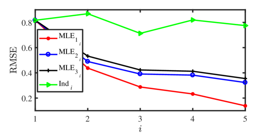
Figure 3: RMSE $\sigma_{rmse}$ of the MLE-based collaborative estimators. Here, $K=5$ and $N=20$.

6.2 Demonstration of the collaborative CS scheme

In this section, we will demonstrate the performance of the notion of collaborative CS scheme (as shown in Fig. 1) and compare it with that of traditional ones.

Through the experiments for this part, we set the number of dictionaries $K=5$. Each training data $\bm{X}_{i}\in\Re^{N\times J_{0}}$ ($i\in[K]$) is obtained by 1) randomly extracting $15$ non-overlapping patches (the dimension of each patch is $8\times 8$) from each of 400 images in the LabelMe [47] training data set, and 2) arranging each patch of $8\times 8$ as a vector of $64\times 1$. Such a setting implies $N=64$ and $J_{0}=15\times 400=6000$. For each training data set $X_{i}$, we apply the K-SVD algorithm to obtain a sparsifying dictionary $\bm{\Psi}_{KSVD_{i}}\in\Re^{N\times L_{0}}$ with $L_{0}=100$ and a given sparsity level $\kappa=4$. We also apply the K-SVD algorithm for the entire training data $\underline{\bm{X}}=\begin{bmatrix}\bm{X}_{1}&\cdots&\bm{X}_{i}&\cdots&\bm{X}_{K}\end{bmatrix}$ to obtain a sparsifying dictionary $\bm{\Psi}_{KSVD}\in\Re^{N\times L}$ with $L=L_{0}$ and $\bm{\Psi}_{\widetilde{KSVD}}\in\Re^{N\times L^{\prime}}$ with $L^{\prime}=23^{2}=529$ (such that $L^{\prime}$ is greater than $KL_{0}=500$). We then generate a random $M\times N$ sensing matrix $\bm{\Phi}$. The CS systems with $(\bm{\Phi},\bm{\Psi}_{KSVD_{i}})$, $(\bm{\Phi},\bm{\Psi}_{KSVD})$ and $(\bm{\Phi},\bm{\Psi}_{\widetilde{KSVD}})$ are then respectively denoted by $\text{CS}_{Rdm_{i}}$, $\text{CS}_{Rdm}$ and $\text{CS}_{\widetilde{Rdm}}$. For any image represented by matrix $\bm{H}$, we apply CS system $\text{CS}_{Rdm_{i}}$ to compress it and use $\bm{H}_{i}$ to denote the output of each CS system. As demonstrated in the last section, we take the average of each CS system for the collaborative CS system. That is, the collaborative CS system (denoted by $\text{CCS}_{Rdm}$) has the output $\widehat{\bm{H}}=\frac{1}{K}\sum_{i=1}^{K}\bm{H}_{i}$. For convenience, we utilize $\text{CCS}_{Rdm_{i}}$ to denote the collaborative CS system that fuses the estimates from the first $i$ CS systems, i.e., with the output $\widehat{\bm{H}}_{i}=\frac{1}{i}\sum_{m=1}^{i}\bm{H}_{m}$. Clearly, $\widehat{\bm{H}}=\widehat{\bm{H}}_{K}$.

The reconstruction accuracy is evaluated in terms of peak signal-to-noise ratio (PSNR), defined as

$$\sigma_{psnr}:=10\times\log_{10}\left(\frac{\left(2^{r}-1\right)^{2}}{\sigma_{mse}}\right),$$

where $r=8$ bits per pixel and $\sigma_{mse}$ for images $\bm{H},\widehat{\bm{H}}\in\Re^{N_{1}\times N_{2}}$ (where $\widehat{\bm{H}}$ is an estimate of $\bm{H}$) defined as

$$\sigma_{mse}:=\frac{1}{N_{1}\times N_{2}}\|\bm{H}-\widehat{\bm{H}}\|^{2}_{F}.$$

As illustrated in Fig. 1, the CS system first divides the input image into a number of non-overlapping $8\times 8$ patches, and then compresses each patch. Once all the patches are recovered, we concatenate them into an image. Fig. 4 shows the PSNR $\sigma_{psnr}$ of the CS systems $\text{CS}_{Rdm_{i}}$ and $\text{CCS}_{Rdm_{i}}$ when applied to the image ‘Plane’. Table 1 provides $\sigma_{psnr}$ for the CS systems $\text{CS}_{Rdm_{i}}$, $\text{CS}_{Rdm}$, $\text{CS}_{\widetilde{Rdm}}$ and $\text{CCS}_{Rdm}$ tested with the twelve images. We also examine the performance with the test data from LabelMe [47]: we randomly extract $15$ non-overlapping patches (the dimension of each patch is $8\times 8$) from each of 400 images in the LabelMe [47] test data set and arrange each patch of $8\times 8$ as a vector of $64\times 1$. Fig. 5 displays the visual effects of image ‘Plane’ for the CS systems $\text{CS}_{Rdm_{i}}$ and $\text{CCS}_{Rdm}$.

Remark 6.2:

• It is observed from Fig. 4 that the performance of the CCS system gets improved with the number of CS systems fused increasing. This coincides with that observed from the experiments just conducted using synthetic data and the expectations induced from the theoretical results in Section 2.1;

• Table 1 also demonstrates the advantages of $\text{CCS}_{Rdm}$. It is of great interest to note that $\text{CCS}_{Rdm}$ has still much better performance than $\text{CS}_{Rdm}$ whose dictionary is learned with the same size as those used in fusion and all the training data $\underline{\bm{X}}$;

• It is interesting to note from Table 1 that $\text{CS}_{\widetilde{Rdm}}$, though with a dictionary $\bm{\Psi}_{\widetilde{KSVD}}$ of dimension higher than $KL_{0}$, even does not outperform $\text{CS}_{Rdm}$. This, as conjectured before and one of the arguments for the proposed CCS framework, is due to the fact that the mutual coherence of the dictionary $\bm{\Psi}$ and hence the equivalent one $\bm{A}$ gets higher when the dimension increases and consequently, the signal reconstruction accuracy decreases.

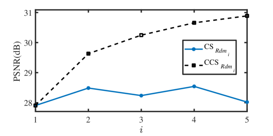
Figure 4: PSNR $\sigma_{psnr}$ of CS systems and collaborative CS systems for image ‘Plane’.

(a)

(b)

(c)

(d)

Figure 5: The original ’Plane’ and reconstructed images from their CS samples with $M=20$ and $\kappa=4$. (a) The original; (b) $\text{CS}_{Rdm_{1}}$; (c) $\text{CS}_{Rdm}$; (d) $\text{CCS}_{Rdm}$.

Table 1: Statistics of $\sigma_{psnr}$(dB) for images processed with $M=20,N=64,L_{0}=100,\kappa=4$, and $K=5$.

	Baboon	Boat	Child	Couple	Crowd	Elanie	Finger	Lake	Lax	Lena	Man	Plane	Test data [47]
$\text{CS}_{Rdm_{1}}$	22.11	26.79	31.03	26.90	27.51	29.45	23.38	25.83	22.49	29.65	27.36	27.91	27.17
$\text{CS}_{Rdm_{2}}$	22.06	26.63	31.08	26.95	27.55	29.37	23.17	25.87	22.51	29.43	27.37	28.49	27.19
$\text{CS}_{Rdm_{3}}$	22.03	26.73	31.04	26.98	27.45	29.28	23.45	25.81	22.50	29.59	27.28	28.24	27.25
$\text{CS}_{Rdm_{4}}$	22.21	26.81	31.05	26.98	27.53	29.39	23.81	26.00	22.55	29.74	27.45	28.54	27.18
$\text{CS}_{Rdm_{5}}$	22.10	26.67	31.10	26.92	27.59	29.56	23.51	25.92	22.54	29.61	27.41	28.02	27.12
$\text{CS}_{Rdm}$	22.39	27.24	31.70	27.51	28.31	29.78	24.31	26.46	22.77	30.32	27.89	29.22	27.78
$\text{CS}_{\widetilde{Rdm}}$	22.14	26.86	31.16	27.08	27.84	29.40	23.68	26.02	22.51	29.75	27.49	28.83	27.45
$\text{CCS}_{Rdm}$	23.78	28.86	33.45	29.09	30.04	31.10	26.48	28.07	24.14	31.93	29.41	30.89	29.38

The excellent performance of CCS system can also be explained as follows. The model (12) suggests that for any patch $\bm{x}$, the following holds

$$||\widehat{\bm{x}}-\bm{x}||^{2}_{2}=||\sum^{K}_{i=1}\omega_{i}(\bm{x}_{i}-\bm{x})||^{2}_{2}\leq\frac{\sum^{K}_{i=1}||\bm{x}_{i}-\bm{x}||^{2}_{2}}{K}$$

when setting $\omega_{i}=1/K,\leavevmode\nobreak\ \forall\leavevmode\nobreak\ i$. As each dictionary has limited capacity of representation, the corresponding CS system may yield excellent performance for some of the patches (of the image), but very poor one for the others. The inequality above implies that for any patch, the variance of the reconstructed one by the CCS system is always smaller than the average of those by the $K$ individual CS systems. As PSNR is evaluated over all the patches, from a statistical point of view the PSNR of the proposed CCS scheme is better than that of any single CS system.

6.3 Performance of the optimized collaborative CS systems

With the obtained training data $\underline{\bm{X}}$, we now examine the performance of the CCS system with sensing matrix and dictionaries simultaneously learned by solving (33) with $\alpha=0.2$, $\beta=1$, $\nu_{1}=\nu_{2}=\nu_{3}=10^{-4}$, $b=10\|\underline{\bm{X}}\|_{\infty}$ and $\nu_{4}=\frac{1}{3(\alpha+\beta+1)L_{0}}$ as suggested by (45). We run the proposed Algorithm 1 with $N_{ite}=30$ iterations to solve (33). As (33) is highly nonconvex, a suitable choice of initialization for Algorithm 1 may result in a better solution. We utilize the DCT matrix as the initialization for each dictionary $\bm{\Psi}_{i}$. We then take the first $M$ left singular vectors of the dictionary as the initialization for the sensing matrix. We conducted the experiments with several type of initializations (like the DCT matrix and the one by randomly selecting a number of training signals for the initialization of the dictionary), and we observed the resulted CCS systems have very similar performance. We defer the thorough investigation of the robustness to the initialization of Algorithm 1 to future work.

In this section, this learned CCS system along with the plain averaging for fusion strategy is simply denoted by CCS. Fig. 6(a) shows the convergence behavior of the objective function $\underline{\varrho}$ as iteration $k$ goes, while Fig. 6(b) displays $\sigma_{psnr}$(dB) for the test data from LabelMe [47] as iteration $k$ goes. Here, $\sigma_{psnr}(k)$ is computed with the test data that is processed using the CCS system obtained at the $k$th iteration of the proposed algorithm. Note that we display Fig. 6(b) only to demonstrate the potential relationship between the objective value $\underline{\varrho}$ defied in (57) and the actual performance of the CCS system and that the test data is not involved in the procedure of training the CCS system. We also show the iterates change $\|\bm{W}_{k}-\bm{W}_{k-1}\|_{F}^{2}$ (recall that $\bm{W}_{k}=(\bm{\Phi}_{k},\underline{\bm{\Psi}}_{k},\underline{\bm{S}}_{k})$) as the iteration $k$ goes in Fig. 6(c). In Figs. 6, we set the number of iterations $N_{ite}=50$ to better illustrate the convergence of Algorithm 1. Finally, with the learned CCS system, we display the normalized version $\overline{\bm{\Gamma}}$ of the correlation matrix $\bm{\Gamma}$ estimated using the test data from LabelMe [47]. In particular, let $\bm{H}\in\Re^{64\times 6000}$ denote the set of test data from LabelMe [47] and $\widehat{\bm{H}}_{1},\ldots,\widehat{\bm{H}}_{K}$ be $K$ estimates of $\bm{H}$ with the learned CCS system. Then the covariance matrix $\bm{\Gamma}$ is estimated using the errors $\begin{bmatrix}(\bm{H}-\widehat{\bm{H}}_{1})^{\cal T}&\cdots&(\bm{H}-\widehat{\bm{H}}_{K})^{\cal T}\end{bmatrix}^{\cal T}$. As seen from Fig. 7, the estimation errors $\{\bm{H}-\widehat{\bm{H}}_{i}\}$, each consisting of sparse representation errors of image signals and these caused by the reconstruction algorithm, are generally correlated to each other.

We now compare the CCS with other CS systems. The CS systems CS_Elad, CS_Classic, CS_TKK, CS_LZYCB, and CS_f are the ones with the learned dictionary $\bm{\Psi}_{KSVD}$ obtained using the K-SVD method [3] and the sensing matrix $\bm{\Phi}\in\Re^{M\times N}$ designed respectively via the methods in [27], [34], [37], [51], and [55], among which the first four methods are all based on minimizing the average coherence of the equivalent dictionary, while the last one given in [34] designs the sensing matrix based on an alternative measure that also takes the sparse representation error into account and hence leads to a more robust CS system than the others. The CS system $\text{CS}_{DCS}$ is the one with the sensing matrix and dictionary that are simultaneously designed with the training data $\underline{\bm{X}}$ using the method in [26].

Table 2 provides the performance of these CS systems for the same twelve images and the test data from LabelMe [47]. Fig. 8 displays the visual effects of image ‘Plane’ for these CS systems. Finally, we list the time used for the algorithms to simultaneously learning the sensing matrix and the dictionary. The CPU time for learning the CCS system with Algorithm 1 is $565$ seconds, while it takes $502$ seconds for learning CS_DCS. As a comparison, the K-SVD algorithm spends $424$ seconds to learn the dictionary $\bm{\Psi}_{KSVD}$. In other words, the other CS systems (like CS_Elad and CS_Classic) that first learn the dictionary (with the K-SVD algorithm) and then design the sensing matrix require at least $424$ seconds. We note that all the experiments are not conducted with the parallel computing strategy.

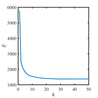
(a)

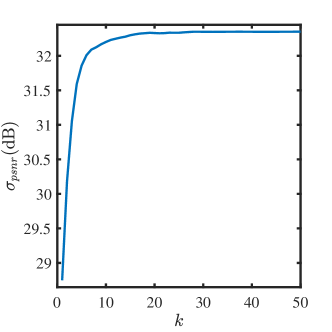
(b)

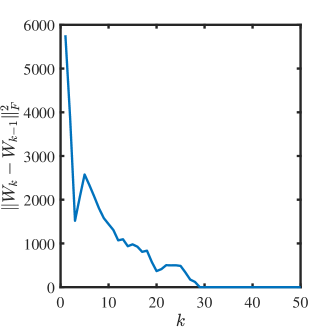
(c)

Figure 6: Evolution of (a) the cost function $\underline{\varrho}(\bm{W}_{k})$ where $\bm{W}_{k}=(\bm{\Phi}_{k},\underline{\bm{\Psi}}_{k},\underline{\bm{S}}_{k})$, (b) the PSNR $\sigma_{psnr}$(dB) for the test data from LabelMe [47], and (c) the iterates change $\|\bm{W}_{k}-\bm{W}_{k-1}\|_{F}^{2}$ with $K=5$.

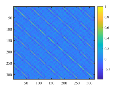
Figure 7: Illustration of the correlation matrix $\overline{\bm{\Gamma}}$ obtained with the test data from LabelMe [47].

Table 2: Statistics of $\sigma_{psnr}$(dB) for images processed with $M=20,N=64,L_{0}=100,\kappa=4$, and $K=5$.

	Baboon	Boat	Child	Couple	Crowd	Elanie	Finger	Lake	Lax	Lena	Man	Plane	Test data [47]
$\text{CS}_{Elad}$	12.11	16.55	25.38	19.40	22.67	14.51	20.94	14.98	10.86	21.52	18.68	23.69	16.57
$\text{CS}_{Classic}$	9.39	13.78	22.79	16.69	20.27	11.83	18.91	12.26	8.11	18.78	15.88	21.26	12.87
$\text{CS}_{TKK}$	11.93	16.31	25.03	19.02	22.28	14.32	20.39	14.60	10.68	21.19	18.34	23.32	14.85
$\text{CS}_{LZYCB}$	8.15	12.54	21.64	15.52	19.22	10.73	17.98	11.08	6.90	17.67	14.82	20.11	12.19
$\text{CS}_{DCS}$	25.35	30.39	34.74	30.58	31.45	32.62	27.39	29.59	25.74	33.38	30.87	32.50	30.39
$\text{CS}_{f}$	24.85	30.04	34.70	30.16	31.46	32.18	27.44	29.42	25.27	33.01	30.61	32.45	30.19
CCS	26.25	31.57	36.42	31.92	33.31	33.36	29.98	31.07	26.44	34.73	32.03	34.18	32.32
$\text{CCS}_{8}$	26.34	31.70	36.62	32.05	33.50	33.42	30.29	31.22	26.55	34.89	32.16	34.42	32.45

(a)

(b)

(c)

(d)

Figure 8: The reconstructed ’Plane’ images from their CS samples with $M=20$ and $\kappa=4$. (a) $\text{CS}_{DCS}$; (b) $\text{CS}_{f}$; (c) $\text{CS}_{etf}$; (d) CCS.

Remark 6.3:

• Comparing Fig. 6(a) and Fig. 6(b), we observe that the PSNR increases when the objective function decreases. We also observe from Fig. 6(c) that the change of iterates $\|\bm{W}_{k}-\bm{W}_{k-1}\|_{F}^{2}$ converges (almost) to 0 after 50 iterations. These confirm the convergence analysis of the proposed Algorithm 1 given in Section 5.2 and demonstrates that the objective function $\underline{\varrho}$ is a good surrogate for the performance of the CS systems in terms of reconstruction accuracy;

• It is observed from Tables 1 and 2 that the CS systems CS_Elad, CS_Classic, CS_TKK, and CS_LZYCB yield a performance even poorer than those that use a random sensing matrix. This is due to the fact that the sensing matrices in the former are optimized with the assumption that the sparse representation errors of signals are very small, which is not the case for images at all;

• As the sensing matrices used in CS_f and CS_DCS are optimized with the sparse representation error taken into account, they perform much better than those using a random sensing matrix and even better than the CCS system CS_Rdm in which the sensing matrix is randomized and all the dictionaries are independently designed using the K-SVD algorithm;

• The superiority of our optimized CCS system CCS is again demonstrated clearly. Compared with CS_Rdm (see TABLE 1), it is basically 2.5 dB better in terms of $\sigma_{psnr}$. This demonstrates clearly the importance of the proposed joint optimization in designing CCS systems. Furthermore, the optimized CCS system CCS yields a performance much better than CS_f and CS_DCS. The amount of improvement can be further increased if the number of CS systems fused in the CCS system increases. With the $5\times 6000=30,000$ samples in the obtained training data matrix $\underline{\bm{X}}$, a CCS system with $K=8$, denoted as CCS₈, is also obtained and its performance is better than the optimized CCS system CCS with $K=5$ by a amount of 0.15 dB on average. See Table 2.

7 Conclusion

Based on the MLE principle, a collaborative estimation framework has been derived. It is shown that by fusing several estimators the collaborative estimator yields a better an estimate than any of the individual estimators when the estimation errors of these estimators are not very correlated. As an application to CS, the CCS scheme has been raised and analyzed, which consists of a bank of $K$ CS systems that share the same sensing matrix. A measure has been proposed, which allows us to simultaneously optimize the sensing matrix and all the $K$ dictionaries. For solving the corresponding optimal CCS system problem, an alternating minimization-based algorithm has been derived with guaranteed convergence. Experiments with synthetic data and real images showed that the proposed optimized CCS systems outperform significantly the traditional CS systems in terms of signal reconstruction accuracy.

In practice, the exact statistical properties can not be obtained. It is an interesting topic to investigate how to learn a collaborative estimator. It is also of interest to develop distributed methods for efficiently implementing the proposed algorithm [33, 45]. Developing alternating minimization-based algorithms with guaranteed convergence is still an important topic in the circumstances, where non-convex optimizations are confronted. The results achieved in the paper seem useful to this topic. Works in these directions are on-going.

Appendix A Proof of Lemma 4.1

Proof A.1 (Proof of Lemma 4.1).

First of all, let $\varrho(\bm{\Phi},\bm{\Psi},\bm{S},\bm{X})$ and $\bm{G}(\bm{\Psi},\bm{S},\bm{X})$ be the same as defined before in (32) and (39), respectively. With $\bm{\Phi}\in{\cal O}_{M,N}$, that is $\bm{\Phi}\bm{\Phi}^{\cal T}={\bf I}_{M}$, it can be shown that

$$\varrho(\bm{\Phi},\bm{\Psi},\bm{S},\bm{X})=-\operatorname{trace}[\bm{\Phi}^{\cal T}\bm{\Phi}\bm{G}(\bm{\Psi},\bm{S},\bm{X})]+ct,$$

where $ct$ is independent of $\bm{\Phi}$. Thus, (36) is equivalent to

$$\bm{\Phi}_{k} =\mathop{\rm argmax}_{\bm{\Phi}\in{\cal O}_{M,N}}\left\{\operatorname{trace}\left[\bm{\Phi}^{\cal T}\bm{\Phi}\left(\sum_{i=1}^{K}\bm{G}\left(\bm{\Psi}_{i,k-1},\bm{S}_{i,k-1},\bm{X}_{i}\right)+2\nu\bm{\Phi}_{k-1}^{\cal T}\bm{\Phi}_{k-1}\right)\right]:=\eta\right\}.$$

It then follows from the ED of $\widetilde{\bm{G}}:=\sum_{i=1}^{K}\bm{G}(\bm{\Psi}_{i,k-1},\bm{S}_{i,k-1},\bm{X}_{i})+2\nu\bm{\Phi}_{k-1}^{\cal T}\bm{\Phi}_{k-1}=\bm{V}_{\tilde{\bm{G}}}{\bf\Pi}\bm{V}_{\tilde{\bm{G}}}^{\cal T}$ and $\bm{\Phi}=\bm{U}\left[\begin{array}[]{cc}{\bf I}_{M}&{\bf 0}\end{array}\right]\bm{V}^{\cal T}$ - an SVD of $\bm{\Phi}$ due to $\bm{\Phi}\in{\cal O}_{M,N}$ that

$$\eta =\operatorname{trace}\left[\tilde{\bm{V}}^{\cal T}{\bf\Pi}\tilde{\bm{V}}\left[\begin{array}[]{cc}{\bf I}_{M}&{\bf 0}\\ {\bf 0}&{\bf 0}\end{array}\right]\right]=\sum^{M}_{n=1}\bm{Q}(n,n),$$

where $\tilde{\bm{V}}:={\bf V}^{\cal T}_{\tilde{\bm{G}}}\bm{V}$ and $\bm{Q}:=\tilde{\bm{V}}^{\cal T}{\bf\Pi}\tilde{\bm{V}}$.

Without loss of generality, assume that the diagonal elements $\{\pi_{n}\}$ of ${\bf\Pi}$ satisfy $\pi_{n}\geq\pi_{n+1},\leavevmode\nobreak\ \forall\leavevmode\nobreak\ n$. According to [37] (see the proof of Theorem 3 there), one has

$$\eta =\sum^{M}_{n=1}\bm{Q}(n,n)\leq\sum^{M}_{n=1}\pi_{n}.$$

Thus, $\eta$ is maximized if $\tilde{\bm{V}}$ is of the following form

(66) $$\tilde{\bm{V}}=\left[\begin{array}[]{cc}\tilde{\bm{V}}_{11}&\bf 0\\ \bf 0&\tilde{\bm{V}}_{22}\end{array}\right],$$

where both $\tilde{\bm{V}}_{11}\in{\cal O}_{M}$ and $\tilde{\bm{V}}_{22}\in{\cal O}_{N-M}$ are arbitrary. Consequently, the optimal sensing matrix is given by

$$\bm{\Phi}_{k}=\bm{U}\left[\begin{array}[]{cc}{\bf I}_{M}&{\bf 0}\end{array}\right]\tilde{\bm{V}}^{\cal T}\bm{V}^{\cal T}_{\tilde{\bm{G}}},$$

where $\tilde{\bm{V}}$ is of form given by (66) and $\bm{U}\in{\cal O}_{M}$ is arbitrary. Clearly, $\tilde{\bm{V}}={\bf I}_{N}$ yields one of the solutions, that is (40).

Appendix B Proof of Lemma 5.1

The proof needs the concept of Fréchet subdifferential, which is given in the following definition.

Definition B.1.

Let $g(\bm{x}):\Re^{N}\rightarrow\Re\cup\{\infty\}$ be a proper lower semi-continuous function in $\bm{x}\in\Re^{N}$.

• The domain of $g(\bm{x})$ is defined by $\text{dom}_{g}:=\{\bm{x}\in\Re^{N}:g(\bm{x})<\infty\}$.

• The Fréchet subdifferential $\partial g$ is defined by

  $$\partial g(\bm{x})=\left\{\bm{z}:\lim_{\bm{y}\rightarrow\bm{x}}\inf\frac{g(\bm{y})-g(\bm{x})-\langle\bm{z},\bm{y}-\bm{x}\rangle}{\|\bm{x}-\bm{y}\|_{2}}\geq 0\right\}$$

  for any $\bm{x}\in\text{dom}_{g}$ and $\partial g(\bm{x})=\emptyset$ if $\bm{x}\notin\text{dom}_{g}$, where $<,>$ denotes the inner product of two vectors.

• For each $\bm{x}\in\text{dom}_{g}$, $\bm{x}$ is called the stationary point of $g(\bm{x})$ if it satisfies $\bm{0}\in\partial g(\bm{x})$.
  

When $g(\bm{x})$ is differentiable at $\bm{x}$, it is clear that the gradient of $g(\bm{x})$ satisfies: $\nabla g(\bm{x})\in\partial g(\bm{x})$.

The OMP algorithm is practically used for solving (59). Under certain conditions (like the mutual coherence or the RIP) on $\bm{A}$, such an algorithm can guarantee to recover the $\kappa$-sparse solution $\bm{s}^{\star}$ if $\bm{y}=\bm{A}\bm{s}^{\star}$ [23, 49]. It is outlined in Algorithm 3, where the set of positions of the nonzero entries of $\bm{s}$ is referred to as the support of $\bm{s}$, denoted by $\text{supp}(\bm{s})$, and $\bm{s}(\Lambda)$ denotes the elements of $\bm{s}$ indexed by $\Lambda$.

Algorithm 3 OMP algorithm for solving (59)

Initialization: set $\bm{s}_{0}=\bm{0},\bm{r}_{0}=\bm{y},\Lambda_{0}=\emptyset$.
Begin $j=0,1,\cdots,\kappa-1$

• identify the support:

  (67) $$\begin{split}\bm{h}_{j}=\bm{A}^{\cal T}\bm{r}_{j},\ \Lambda_{j+1}=\Lambda_{j}\cup\{\arg\max_{l}|\bm{h}_{j}(l)|\}\leavevmode\nobreak\ \text{(choose one if multiple maxima exist).}\end{split}$$

• update the estimate and the residual:

  (68) $$\bm{s}_{j+1}=\mathop{\rm argmin}_{\bm{z}:\text{supp}(\bm{z})\subset\Lambda_{j+1}}\|\bm{y}-\bm{A}\bm{z}\|^{2}_{2},\ \bm{r}_{j+1}=\bm{y}-\bm{A}\bm{s}_{j+1}.$$

End
Output: $\widehat{\bm{s}}=\bm{s}_{\kappa}$.

Proof B.2 (Proof of Lemma 5.1).

First note that the OMP algorithm iteratively finds an atom from $\bm{A}$ that has not been selected before, is not within the subspace spanned by the selected atoms, and best fits the residual vector $\bm{r}$. Thus, if $\bm{h}_{j}\neq\bm{0}$, we know that the atoms of $\bm{A}$ indexed by $\Lambda_{j+1}$ are linearly independent and $\bm{s}_{j+1}(\Lambda_{j+1})$ has no zero element.

We first suppose $\bm{h}_{\kappa-1}\neq\bm{0}$, which implies that $\bm{h}_{\kappa-1}$ has at least one non-zero elements. In this case, we know $\widehat{\bm{s}}(\Lambda_{\kappa})$ has no zero element. Thus, when $\bm{s}\rightarrow\widehat{\bm{s}}$, we have $\Lambda_{\kappa}\subset\text{supp}(\bm{s})$. Now if $\Lambda_{\kappa}=\text{supp}(\bm{s})$, we know $g(\bm{s})\geq g(\widehat{\bm{s}})$ since $\widehat{\bm{s}}=\mathop{\rm argmin}_{\bm{z}:\text{supp}(\bm{z})=\Lambda_{\kappa}}\|\bm{y}-\bm{A}\bm{z}\|^{2}_{2}$. Otherwise $\Lambda_{\kappa}\subset\text{supp}(\bm{s})$, we have $g(\bm{s})=\infty$ since $\bm{s}$ has more than $\kappa$ number of non-zero elements. Thus, we conclude

$$\lim_{\bm{s}\rightarrow\widehat{\bm{s}}}\inf\frac{g(\bm{s})-g(\widehat{\bm{s}})-\langle\bm{0},\bm{s}-\widehat{\bm{s}}\rangle}{\|\bm{s}-\widehat{\bm{s}}\|}\geq 0,$$

which implies $\bm{0}\in\partial g(\widehat{\bm{s}})$.

Now if $\bm{h}_{\kappa-1}=\bm{0}$, which means that $\bm{r}_{\kappa-1}$ is orthogonal to $\bm{A}$. We can decompose $\bm{y}$ into two parts, $\bm{y}=\bm{y}_{1}+\bm{y}_{2}$, where $\bm{y}_{1}$ is within the subspace spanned by $\bm{A}(\Lambda_{\kappa-1})$, and $\bm{y}_{2}$ is orthogonal to the subspace spanned by $\bm{A}$. Thus, in this case $\bm{s}_{\kappa-1}$ is the global solution to (59) (and also to $\min_{\bm{s}}\|\bm{A}\bm{s}-\bm{y}\|^{2}_{2}$), which implies that $\widehat{\bm{s}}=\bm{s}_{\kappa}$ is also the global solution to (59). Thus, it follows from the optimality condition that $\bm{0}\in\partial g(\widehat{\bm{s}})$.

Appendix C Proof of Theorem 5.2

Proof C.1.

Note that $\underline{\varrho}(\bm{\Phi},\underline{\bm{\Psi}},\underline{\bm{S}})$ defined before can be considered as a function of three matrix-variables, and it has a (Fréchet) subdifferential of $\underline{\varrho}$ with respect to each variable, say $\underline{\bm{\Psi}}$. Such subdifferential is denoted as $\partial_{\underline{\bm{\Psi}}}\underline{\varrho}$. In the same way, $\partial_{\bm{\psi}_{i,\ell}}\underline{\varrho}$ denotes the (Fréchet) subdifferential of $\underline{\varrho}$ with respect to the $\ell$-th column in the dictionary $\bm{\Psi}_{i}$. All these apply to the notations for gradient functions. Note that due to $\underline{\varrho}(\bm{\Phi},\underline{\bm{\Psi}},\underline{\bm{S}})=\sum_{i=1}^{K}\varrho(\bm{\Phi},\bm{\Psi}_{i},\bm{S}_{i})$, we have $\nabla_{\bm{\psi}_{i,\ell}}\underline{\varrho}(\bm{\Phi},\underline{\bm{\Psi}},\underline{\bm{S}})=\nabla_{\bm{\psi}_{\ell}}\varrho(\bm{\Phi},\bm{\Psi}_{i},\bm{S}_{i})$.

Let $\bm{W}_{k}=(\bm{\Phi}_{k},\underline{\bm{\Psi}}_{k},\underline{\bm{S}}_{k})$ be the point generated with our proposed algorithm at the $k$-th iteration and $\bm{\psi}_{i,k,\ell}$ denote the $\ell$-th column of $\bm{\Psi}_{i,k}$ - the $i$th dictionary corresponding to $\underline{\bm{\Psi}}_{k}$. Define

$$\bm{\Psi}_{i,k,\ell}/\bm{\psi}:=\begin{bmatrix}\bm{\psi}_{i,k,1}&\cdots\bm{\psi}_{i,k,\ell-1}&\bm{\psi}&\bm{\psi}_{i,k-1,\ell+1}&\bm{\psi}_{i,k-1,L_{0}}\end{bmatrix}.$$

With this definition, we have $\bm{\Psi}_{i,k,L_{0}}/\bm{\psi}_{i,k,L_{0}}=\bm{\Psi}_{i,k}$ and $\bm{\Psi}_{i,k,1}/\bm{\psi}_{i,k-1,1}=\bm{\Psi}_{i,k-1}$.

Since the sets $\mathcal{O}_{M,N},\mathcal{U}_{N},\mathcal{S}_{\kappa,b}$ all are bounded and $\underline{\varrho}$ is smooth, it is clear that $\underline{\varrho}$ has Lipschitz continuous gradient [15], i.e., there exists a constant $L_{c}>0$ such that

(69) $$\left\|\nabla\underline{\varrho}(\bm{\Phi},\underline{\bm{\Psi}},\underline{\bm{S}})-\nabla\underline{\varrho}(\bm{\Phi}^{\prime},\underline{\bm{\Psi}}^{\prime},\underline{\bm{S}}^{\prime})\right\|_{F}\leq L_{c}\left\|(\bm{\Phi},\underline{\bm{\Psi}},\underline{\bm{S}})-(\bm{\Phi}^{\prime},\underline{\bm{\Psi}}^{\prime},\underline{\bm{S}}^{\prime})\right\|_{F}$$

for all $\bm{\Phi},\bm{\Phi}^{\prime}\in\mathcal{O}_{M,N},\underline{\bm{\Psi}},\underline{\bm{\Psi}}^{\prime}\in\mathcal{U}_{N}^{KL_{0}}$ and $\underline{\bm{S}},\underline{\bm{S}}^{\prime}\in\mathcal{S}_{\kappa,b}^{KJ_{0}}$.

Proof of Part $(i)$ of Theorem 5.2: As $\bm{\Phi}_{k}$ is the solution of (36), we have

$$\underline{\varrho}(\bm{\Phi}_{k},\underline{\bm{\Psi}}_{k-1},\underline{\bm{S}}_{k-1})+\nu_{1}\|\bm{\Phi}_{k}^{\cal T}\bm{\Phi}_{k}-\bm{\Phi}_{k-1}^{\cal T}\bm{\Phi}_{k-1}\|_{F}^{2}\leq\underline{\varrho}(\bm{\Phi}_{k-1},\underline{\bm{\Psi}}_{k-1},\underline{\bm{S}}_{k-1}),$$

which implies that

(70) $$\begin{split}\underline{\varrho}(\bm{\Phi}_{k-1},\underline{\bm{\Psi}}_{k-1},\underline{\bm{S}}_{k-1})-\underline{\varrho}(\bm{\Phi}_{k},\underline{\bm{\Psi}}_{k-1},\underline{\bm{S}}_{k-1})&\geq\nu_{1}\|\bm{\Phi}_{k}^{\cal T}\bm{\Phi}_{k}-\bm{\Phi}_{k-1}^{\cal T}\bm{\Phi}_{k-1}\|_{F}^{2}\\ &\geq\nu_{1}\|\bm{\Phi}_{k}-\bm{\Phi}_{k-1}\|_{F}^{2},\end{split}$$

where the last inequality follows from [38, Lemma 3.4] by noting that $\bm{\Phi}_{k}$ is updated as (61).

Keeping the definition of $\bm{\psi}_{i,k,\ell}$ in mind, we obtain

$$\varrho(\bm{\Phi}_{k},\bm{\Psi}_{i,k,\ell}/\bm{\psi}_{i,k,\ell},\bm{S}_{i,k-1})+\nu_{2}\|\bm{\psi}_{i,k,\ell}-\bm{\psi}_{i,k-1,\ell}\|^{2}\leq\varrho(\bm{\Phi}_{k},\bm{\Psi}_{i,k,\ell}/\bm{\psi}_{i,k-1,\ell},\bm{S}_{i,k-1})$$

for all $i\in[K]$ and $\ell\in[L_{0}]$. Repeating the above equations for all $\ell\in[L_{0}]$ and summing them up give

(71) $$\varrho(\bm{\Phi}_{k},\bm{\Psi}_{i,k-1},\bm{S}_{i,k-1})-\varrho(\bm{\Phi}_{k},\bm{\Psi}_{i,k},\bm{S}_{i,k-1})\geq\nu_{2}\|\bm{\Psi}_{i,k}-\bm{\Psi}_{i,k-1}\|^{2}_{F}$$

for all $i\in[K]$.

The rest is to show similar sufficient decrease property in terms of $\bm{S}_{i}$. If $\bm{S}_{i,k}$ is updated via the first expression of (42), it is clear that

(72) $$\varrho(\bm{\Phi}_{k},\bm{\Psi}_{i,k},\bm{S}_{i,k-1})-\varrho(\bm{\Phi}_{k},\bm{\Psi}_{i,k},\bm{S}_{i,k})\geq\nu_{3}\|\bm{\Psi}_{i,k}-\bm{\Psi}_{i,k-1}\|^{2}_{F}.$$

Now, we consider the other case that $\bm{S}_{i,k}$ is updated via the 2nd expression of (42). We define the proximal regularization of $\varrho(\bm{\Phi},\bm{\Psi},\bm{S})$ linearized at $\bm{S}^{\prime}$ as

$$\varrho_{\nu^{\prime}}(\bm{\Phi},\bm{\Psi},\bm{S},\bm{S}^{\prime})=\varrho(\bm{\Phi},\bm{\Psi},\bm{S}^{\prime})+\langle\nabla_{\bm{S}}\varrho(\bm{\Phi},\bm{\Psi},\bm{S}^{\prime}),\bm{S}-\bm{S}^{\prime}\rangle+\frac{\nu^{\prime}}{2}\|\bm{S}-\bm{S}^{\prime}\|_{F}^{2}.$$

Due to (44), we have

(73) $$\varrho(\bm{\Phi},\bm{\Psi},\bm{S})\leq\varrho_{2(1+\alpha+\beta)L_{0}}(\bm{\Phi},\bm{\Psi},\bm{S},\bm{S}^{\prime}),\ \forall\ \bm{S}^{\prime}\in\mathcal{S}_{\kappa,b}^{J_{0}}.$$

Note that

(74) $$\begin{split}&\bm{S}_{i,k}=\mathcal{P}_{\bm{S}\in\mathcal{S}_{\kappa,b}^{J_{0}}}\left[\bm{S}_{i,k-1}-\nu_{4}\nabla_{\bm{S}}\varrho(\bm{\Phi}_{k},\bm{\Psi}_{i,k},\bm{S}_{i,k-1})\right]\\ &=\mathop{\rm argmin}_{\bm{S}\in\mathcal{S}_{\kappa,b}^{J_{0}}}\left\|\bm{S}-\left(\bm{S}_{i,k-1}-\nu_{4}\nabla_{\bm{S}}\varrho(\bm{\Phi}_{k},\bm{\Psi}_{i,k},\bm{S}_{i,k-1})\right)\right\|_{F}^{2}\\ &=\mathop{\rm argmin}_{\bm{S}\in\mathcal{S}_{\kappa,b}^{J_{0}}}\varrho(\bm{\Phi}_{k},\bm{\Psi}_{i,k},\bm{S}_{i,k-1})+\langle\nabla_{\bm{S}}\varrho(\bm{\Phi}_{k},\bm{\Psi}_{i,k},\bm{S}_{i,k-1}),\bm{S}-\bm{S}_{i,k-1}\rangle+\frac{1}{2\nu_{4}}\|\bm{S}-\bm{S}_{i,k-1}\|_{F}^{2}\\ &=\mathop{\rm argmin}_{\bm{S}\in\mathcal{S}_{\kappa,b}^{J_{0}}}\varrho_{\frac{1}{\nu_{4}}}(\bm{\Phi}_{k},\bm{\Psi}_{i,k},\bm{S},\bm{S}_{i,k-1}),\end{split}$$

which implies that

$$\varrho_{\frac{1}{\nu_{4}}}(\bm{\Phi}_{k},\bm{\Psi}_{i,k},\bm{S}_{i,k},\bm{S}_{i,k-1})\leq\varrho(\bm{\Phi}_{k},\bm{\Psi}_{i,k},\bm{S}_{i,k-1}).$$

This, together with (73) (by setting $\bm{\Phi}=\bm{\Phi}_{k}$, $\bm{\Psi}=\bm{\Psi}_{i,k}$, $\bm{S}=\bm{S}_{i,k}$ and $\bm{S}^{\prime}=\bm{S}_{i,k-1}$), gives

(75) $$\begin{split}&\varrho(\bm{\Phi}_{k},\bm{\Psi}_{i,k},\bm{S}_{i,k-1})-\varrho(\bm{\Phi}_{k},\bm{\Psi}_{i,k},\bm{S}_{i,k})\geq\varrho_{\frac{1}{\nu_{4}}}(\bm{\Phi}_{k},\bm{\Psi}_{i,k},\bm{S}_{i,k},\bm{S}_{i,k-1})-\varrho_{2(1+\alpha+\beta)L_{0}}(\bm{\Phi}_{k},\bm{\Psi}_{i,k},\bm{S}_{i,k},\bm{S}_{i,k-1})\\ &\geq\frac{1}{2}(\frac{1}{\nu_{4}}-2(1+\alpha+\beta)L_{0})\|\bm{S}_{i,k}-\bm{S}_{i,k-1}\|_{F}^{2}.\end{split}$$

Let

(76) $$c_{1}=\min\{\nu_{1},\nu_{2},\nu_{3},\frac{1}{2}(\frac{1}{\nu_{4}}-2(1+\alpha+\beta)L_{0})\}.$$

Combining (70)-(75), we conclude

$$\varrho(\bm{\Phi}_{k-1},\bm{\Psi}_{i,k-1},\bm{S}_{i,k-1})-\varrho(\bm{\Phi}_{k},\bm{\Psi}_{i,k},\bm{S}_{i,k})\geq c_{1}\|(\bm{\Phi}_{k-1},\bm{\Psi}_{i,k-1},\bm{S}_{i,k-1})-(\bm{\Phi}_{k},\bm{\Psi}_{i,k},\bm{S}_{i,k})\|_{F}^{2},$$

which implies

(77) $$\underline{\varrho}(\bm{\Phi}_{k-1},\underline{\bm{\Psi}}_{k-1},\underline{\bm{S}}_{k-1})-\underline{\varrho}(\bm{\Phi}_{k},\underline{\bm{\Psi}}_{k},\underline{\bm{S}}_{k})\geq c_{1}\|\bm{W}_{k-1}-\bm{W}_{k}\|_{F}^{2}.$$

By repeating the above equation for all $k\geq 1$ and summing them, we have

$$c_{1}\sum_{k=1}^{\infty}\|\bm{W}_{k-1}-\bm{W}_{k}\|_{F}^{2}\leq\underline{\varrho}(\bm{\Phi}_{0},\underline{\bm{\Psi}}_{0},\underline{\bm{S}}_{0})$$

since $\underline{\varrho}(\bm{W}_{k})\geq 0$ for all $k$. Thus, we obtain $\lim_{k\rightarrow\infty}\|\bm{W}_{k-1}-\bm{W}_{k}\|_{F}=0$.

The proof is completed by noting the fact that $\bm{W}_{k}\in{\cal O}_{M,N}\times{\cal U}_{N}^{L_{0}K}\times\mathcal{S}_{\kappa,b}^{KJ_{0}}$ for all $k$ and hence $f(\bm{W}_{k})=\underline{\varrho}(\bm{\Phi}_{k},\underline{\bm{\Psi}}_{k},\underline{\bm{S}}_{k})$.

Proof of Part (ii) of Theorem 5.2: Since the sets $\mathcal{O}_{M,N},\mathcal{U}_{N},\mathcal{S}_{\kappa,b}$ are compact and $\bm{W}_{k}\in{\cal O}_{M,N}\times{\cal U}_{N}^{L_{0}K}\times\mathcal{S}_{\kappa,b}^{KJ_{0}}$ for all $k$, this bounded $\{\bm{W}_{k}\}$, as suggested by the Bolzano-Weiestrass Theorem [12], has at least a convergent subsequence $\{\bm{W}_{k_{m}}\}$ with limit point denoted as $\bm{W}^{\star}$.

Note that $f(\bm{W}_{k})=\underline{\varrho}(\bm{\Phi}_{k},\underline{\bm{\Psi}}_{k},\underline{\bm{S}}_{k})$ and

$$\lim_{k\rightarrow\infty}I_{{\cal O}_{M,N}}(\bm{\Phi}_{k})=\lim_{k\rightarrow\infty}I_{{\cal U}_{N}^{L_{0}K}}(\underline{\bm{\Psi}}_{k})=\lim_{k\rightarrow\infty}I_{\mathcal{S}_{\kappa,b}^{KJ_{0}}}(\underline{\bm{S}}_{k})=0$$

since the sets $\mathcal{O}_{M,N},\mathcal{U}_{N},\mathcal{S}_{\kappa,b}$ are compact, which also implies that $\bm{W}^{\star}\in{\cal O}_{M,N}\times{\cal U}_{N}^{L_{0}K}\times\mathcal{S}_{\kappa,b}^{KJ_{0}}$. Recall that $\{\underline{\varrho}(\bm{\Phi}_{k},\underline{\bm{\Psi}}_{k},\underline{\bm{S}}_{k})\}$, as just shown above, is a non-increasing sequence and is convergent. As well known, its subsequence $\{\underline{\varrho}(\bm{\Phi}_{k_{m}},\underline{\bm{\Psi}}_{k_{m}},\underline{\bm{S}}_{k_{m}})\}$ is also convergent (since $\varrho$ is continuous) and converges to the same limit point:

$$\lim_{k\rightarrow\infty}f(\bm{W}_{k})=\lim_{k_{m}\rightarrow\infty}f(\bm{W}_{k_{m}})=f(\bm{W}^{\star}).$$

We now show that $\bm{W}^{\star}$ is a critical point of $f(\bm{W})$.

Since $\bm{\Phi}_{k}$ is a solution of (36), it should be a stationary point of the problem in the RHS of (36), that is

$$\bm{0}\in\nabla_{\bm{\Phi}}\underline{\varrho}(\bm{\Phi}_{k},\underline{\bm{\Psi}}_{k-1},\underline{\bm{S}}_{k-1})+4\nu_{1}\bm{\Phi}_{k}(\bm{\Phi}_{k}^{\cal T}\bm{\Phi}_{k}-\bm{\Phi}_{k-1}^{\cal T}\bm{\Phi}_{k-1})+\partial I_{{\cal O}_{M,N}}(\bm{\Phi}_{k}).$$

Equivalently,

$$\underbrace{\nabla_{\bm{\Phi}}\underline{\varrho}(\bm{\Phi}_{k},\underline{\bm{\Psi}}_{k},\underline{\bm{S}}_{k})-\nabla_{\bm{\Phi}}\underline{\varrho}(\bm{\Phi}_{k},\underline{\bm{\Psi}}_{k-1},\underline{\bm{S}}_{k-1})-4\nu_{1}\bm{\Phi}_{k}(\bm{\Phi}_{k}^{\cal T}\bm{\Phi}_{k}-\bm{\Phi}_{k-1}^{\cal T}\bm{\Phi}_{k-1})}_{\bm{D}_{\bm{\Phi}_{k}}}\in\partial_{\bm{\Phi}}f(\bm{\Phi}_{k},\underline{\bm{\Psi}}_{k},\underline{\bm{S}}_{k}).$$

To bound $\|\bm{D}_{\bm{\Phi}_{k}}\|_{F}$, first note that

$$\begin{split}&\|\bm{\Phi}_{k}(\bm{\Phi}_{k}^{\cal T}\bm{\Phi}_{k}-\bm{\Phi}_{k-1}^{\cal T}\bm{\Phi}_{k-1})\|_{F}\leq\|\bm{\Phi}_{k}^{\cal T}\bm{\Phi}_{k}-\bm{\Phi}_{k-1}^{\cal T}\bm{\Phi}_{k-1}\|_{F}\\ &=\|\bm{\Phi}_{k}^{\cal T}(\bm{\Phi}_{k}-\bm{\Phi}_{k-1})+(\bm{\Phi}_{k}-\bm{\Phi}_{k-1})^{\cal T}\bm{\Phi}_{k-1}\|_{F}\\ &\leq\|\bm{\Phi}_{k}^{\cal T}(\bm{\Phi}_{k}-\bm{\Phi}_{k-1})\|_{F}+\|(\bm{\Phi}_{k}-\bm{\Phi}_{k-1})^{\cal T}\bm{\Phi}_{k-1}\|_{F}\leq 2\|\bm{\Phi}_{k}-\bm{\Phi}_{k-1}\|_{F},\end{split}$$

where we utilize the inequality $\|\bm{C}\bm{D}\|_{F}\leq\|\bm{C}\|_{2}\|\bm{D}\|_{F}$ and the fact that both $\bm{\Phi}_{k}$ and $\bm{\Phi}_{k-1}$ has spectral norm (i.e., largest singular value) $1$. Also, it follows from the global Lipschitz property of $\underline{\varrho}$ in (69) that

$$\begin{split}\|\nabla_{\bm{\Phi}}\underline{\varrho}(\bm{\Phi}_{k},\underline{\bm{\Psi}}_{k},\underline{\bm{S}}_{k})-\nabla_{\bm{\Phi}}\underline{\varrho}(\bm{\Phi}_{k},\underline{\bm{\Psi}}_{k-1},\underline{\bm{S}}_{k-1})\|_{F}\leq L_{c}\|\bm{\Phi}_{k}-\bm{\Phi}_{k-1}\|_{F}.\end{split}$$

Thus, the term $\|\bm{D}_{\bm{\Phi}_{k}}\|_{F}$ can be bounded as

(78) $$\begin{split}\|\bm{D}_{\bm{\Phi}_{k}}\|_{F}\leq(8\nu_{1}+L_{c})\|\bm{\Phi}_{k}-\bm{\Phi}_{k-1}\|_{F}.\end{split}$$

Similarly, it follows from the definition of $\bm{\psi}_{i,k,\ell}$ that the following holds

$$\begin{split}\bm{0}\in\nabla_{\bm{\psi}_{\ell}}\varrho(\bm{\Phi}_{k},\bm{\Psi}_{i,k,\ell}/\bm{\psi}_{i,k,l},\bm{S}_{i,k-1})+2\nu_{2}\left(\bm{\psi}_{i,k,\ell}-\bm{\psi}_{i,k-1,\ell}\right)+\partial I_{\mathcal{U}_{N}}(\bm{\psi}_{i,k,\ell}).\end{split}$$

Noting that

$$\partial_{\bm{\psi}_{i,\ell}}f(\bm{\Phi}_{k},\underline{\bm{\Psi}}_{k},\underline{\bm{S}}_{k})=\nabla_{\bm{\psi}_{\ell}}\varrho(\bm{\Phi}_{k},\bm{\Psi}_{i,k},\bm{S}_{i,k})+\partial I_{\mathcal{U}_{N}}(\bm{\psi}_{i,k,\ell}),$$

which, together with the above equation, gives

$$\begin{split}\underbrace{\nabla_{\bm{\psi}_{\ell}}\varrho(\bm{\Phi}_{k},\bm{\Psi}_{i,k},\bm{S}_{i,k})-\nabla_{\bm{\psi}_{\ell}}\varrho(\bm{\Phi}_{k},\bm{\Psi}_{i,k,\ell}/\bm{\psi}_{i,k,\ell},\bm{S}_{i,k-1})-2\nu_{2}\left(\bm{\psi}_{i,k,\ell}-\bm{\psi}_{i,k-1,\ell}\right)}_{\bm{D}_{\bm{\psi}_{i,k,\ell}}}\in\partial_{\bm{\psi}_{i,\ell}}f(\bm{\Phi}_{k},\underline{\bm{\Psi}}_{k},\underline{\bm{S}}_{k}).\end{split}$$

Due to the global Lipschitz property of $\underline{\varrho}$ in (69), we have

$$\begin{split}\left\|\nabla_{\bm{\psi}_{\ell}}\varrho(\bm{\Phi}_{k},\bm{\Psi}_{i,k},\bm{S}_{i,k})-\nabla_{\bm{\psi}_{l}}\varrho(\bm{\Phi}_{k},\bm{\Psi}_{i,k,\ell}/\bm{\psi}_{i,k,\ell},\bm{S}_{i,k-1})\right\|_{F}&\leq L_{c}\|(\bm{\Phi}_{k},\bm{\Psi}_{i,k},\bm{S}_{i,k})-(\bm{\Phi}_{k},\bm{\Psi}_{i,k,\ell}/\bm{\psi}_{i,k,\ell},\bm{S}_{i,k-1})\|_{F}\\ &\leq L_{c}(\|\bm{\Psi}_{i,k}-\bm{\Psi}_{i,k-1}\|_{F}+\|\bm{S}_{i,k}-\bm{S}_{i,k-1}\|_{F}),\end{split}$$

which implies that

(79) $$\begin{split}\|\bm{D}_{\bm{\psi}_{i,k,l}}\|_{F}&\leq L_{c}(\|\bm{\Psi}_{i,k}-\bm{\Psi}_{i,k-1}\|_{F}+\|\bm{S}_{i,k}-\bm{S}_{i,k-1}\|_{F})+2\nu_{2}\left\|\bm{\psi}_{i,k,l}-\bm{\psi}_{i,k-1,l}\right\|_{F}\\ &\leq(L_{c}+2\nu_{2})\|\bm{\Psi}_{i,k}-\bm{\Psi}_{i,k-1}\|_{F}+L_{c}\|\bm{S}_{i,k}-\bm{S}_{i,k-1}\|_{F}.\end{split}$$

The rest is to show similar properties for the subdifferential in terms of $\bm{S}_{i}$. If $\bm{S}_{i,k}$ is updated via the first expression of (42), by utilizing Lemma 5.1 (the constraint $\|\bm{S}_{i}\|_{\infty}\leq b$ can be simply incorporated into the analysis), we have

(80) $$\bm{0}\in\partial_{\bm{S}_{i}}f(\bm{\Phi}_{k},\underline{\bm{\Psi}}_{k},\underline{\bm{S}}_{k}).$$

When $\bm{S}_{i,k}$ is updated via the 2nd expression of (42), the optimality condition of (74) gives

$$\bm{0}\in\nabla_{\bm{S}}\varrho(\bm{\Phi}_{k},\bm{\Psi}_{i,k},\bm{S}_{i,k-1})+\frac{1}{\nu_{4}}(\bm{S}_{i,k}-\bm{S}_{i,k-1})+\partial I_{\mathcal{S}_{\kappa,b}^{J_{0}}}(\bm{S}_{i,k}),$$

which implies that

$$\underbrace{\nabla_{\bm{S}}\varrho(\bm{\Phi}_{k},\bm{\Psi}_{i,k},\bm{S}_{i,k})-\nabla_{\bm{S}}\varrho(\bm{\Phi}_{k},\bm{\Psi}_{i,k},\bm{S}_{i,k-1})-\frac{1}{\nu_{4}}(\bm{S}_{i,k}-\bm{S}_{i,k-1})}_{\bm{D}_{\bm{S}_{i,k}}}\in\partial_{\bm{S}_{i}}f(\bm{\Phi}_{k},\underline{\bm{\Psi}}_{k},\underline{\bm{S}}_{k})$$

Similar to (79), we bound $\bm{D}_{\bm{S}_{i,k}}$ as

(81) $$\|\bm{D}_{\bm{S}_{i,k}}\|_{F}\leq(L_{c}+\frac{1}{\nu_{4}})\|\bm{S}_{i,k}-\bm{S}_{i,k-1}\|_{F}.$$

We stack $\bm{D}_{\bm{\Phi}_{k}},\bm{D}_{\bm{\psi}_{i,k,l}}$ and $\bm{0}$ (or $\bm{D}_{\bm{S}_{i,k}}$) into

$$\begin{split}\bm{D}_{k}&=\left(\bm{D}_{\bm{\Phi}_{k}},\bm{D}_{\bm{\psi}_{1,k,1}},\ldots,\bm{D}_{\bm{\psi}_{K,k,L_{0}}},\bm{0}\right),\\ \bm{D}_{k}^{\prime}&=\left(\bm{D}_{\bm{\Phi}_{k}},\bm{D}_{\bm{\psi}_{1,k,1}},\ldots,\bm{D}_{\bm{\psi}_{K,k,L_{0}}},\bm{D}_{\bm{S}_{1,k}},\ldots,\bm{D}_{\bm{S}_{K,k}}\right).\end{split}$$

We have either $\bm{D}_{k}\in\partial f(\bm{\Phi}_{k},\underline{\bm{\Psi}}_{k},\underline{\bm{S}}_{k})$ or $\bm{D}^{\prime}_{k}\in\partial f(\bm{\Phi}_{k},\underline{\bm{\Psi}}_{k},\underline{\bm{S}}_{k})$. Let

(82) $$c_{2}=2(L_{0}+1)L_{c}+2L_{0}\nu_{2}+8\nu_{1}+\frac{1}{\nu_{4}}.$$

It follows from (78)-(81) that

(83) $$\|\bm{D}_{k}\|_{F},\|\bm{D}^{\prime}_{k}\|_{F}\leq c_{2}\|\bm{W}_{k}-\bm{W}_{k-1}\|_{F}.$$

Recalling from (77) that $\lim_{k_{m}\rightarrow\infty}\|\bm{W}_{k_{m}}-\bm{W}_{k_{m}-1}\|_{F}=0$, we have $\lim_{k_{m}\rightarrow\infty}\bm{D}_{k_{m}}=\lim_{k_{m}\rightarrow\infty}\bm{D}^{\prime}_{k_{m}}=\bm{0}$. Owing to the closedness properties of $\partial f(\bm{W}_{k})$, we finally obtain $\bm{0}\in\partial f(\bm{W}^{\star})$. Thus, $\bm{W}^{\star}$ is a critical point of $f(\bm{W})$. This completes the proof of Theorem 5.2.

Appendix D Proof of Theorem 5.3

We first state the definition of Kurdyka-Lojasiewicz (KL) inequality, which is proved to be useful for convergence analysis of the iterates sequence [4, 5, 8, 9, 15].

Definition D.1.

(Kurdyka-Lojasiewicz (KL) inequality [4, 5, 15].) A proper semi-continuous function $g(\bm{x}):\Re^{N}\rightarrow\Re$ is said to satisfy the Kurdyka-Lojasiewicz (KL) inequality, if for any stationary point $\bm{x}^{\star}$ of $g(\bm{x})$, there exist constants $\delta>0,\theta\in[0,1),c>0$ such that

$$\left|g(\bm{x})-g(\bm{x}^{\star})\right|^{\theta}\leq c\leavevmode\nobreak\ \textup{dist}[\partial g(\bm{x}),0],\leavevmode\nobreak\ \leavevmode\nobreak\ \forall\leavevmode\nobreak\ \bm{x}\in\mathbb{B}(\bm{x}^{\star},\delta),$$

where $\mathbb{B}(\bm{x}^{\star},\delta)=\{\bm{x}\in\Re^{n}:\|\bm{x}-\bm{x}^{\star}\|_{2}\leq\delta\}$ and $\textup{dist}[\partial g(\bm{x}),\bm{0}]=\min_{\bm{d}\in\partial g(\bm{x})}\|\bm{d}\|_{2}$ denotes the distance of $\bm{0}$ to the set $\partial g(\bm{x})$.

Proof D.2.

It is clear that $f(\bm{W})$ is a KL function since $\underline{\varrho}(\bm{W})$ is a KL function (as it is an analytical function) and $I_{{\cal O}_{M,N}}(\bm{\Phi})$, $I_{{\cal U}_{N}^{L_{0}K}}(\underline{\bm{\Psi}})$ and $I_{\mathcal{S}_{\kappa,b}^{KJ_{0}}}(\underline{\bm{S}})$ are also KL functions as they are the indicator functions on the sets ${\cal O}_{M,N}$, ${\cal U}_{N}^{L_{0}K}$ and $\mathcal{S}_{\kappa,b}^{KJ_{0}}$ respectively [15].

Let ${\cal H}_{\bm{W}}$ denote the set of accumulation points of $\{\bm{W}_{k}\}$, i.e.,

$${\cal H}_{\bm{W}}=\left\{\overline{\bm{W}}:\exists\ \textup{an increasing sequence of intergers}\ \{k_{m}\}_{m\in\mathbb{N}},\ \textup{s.t.}\lim_{m\rightarrow\infty}\bm{W}_{k_{m}}=\overline{\bm{W}}\right\}.$$

Recall part($ii$) of Theorem 5.2, which states that any element $\bm{W}^{\star}\in{\cal H}_{\bm{W}}$ is a stationary point of $f(\bm{W})$ and $f(\bm{W})$ has the same value at the set ${\cal H}_{\bm{W}}$. Also since the sequence $\{\bm{W}_{k}\}$ is bounded and regular (see (63)), we know that ${\cal H}_{\bm{W}}$ is a nonempty compact connected set and satisfies [15, Lemma 3.5]

(84) $$\lim_{k\rightarrow\infty}\text{dist}[\bm{W}_{k},{\cal H}_{\bm{W}}]=0.$$

First, note that if there exists an integer $k_{0}$ for which $f(\bm{W}_{k_{0}})=f(\bm{W}^{\star})$ with $\bm{W}^{\star}\in{\cal H}_{\bm{W}}$, it follows from (62) and (64) that $\bm{W}_{k}=\bm{W}_{k_{0}}$ for all $k\geq k_{0}$. Thus, $\{\bm{W}_{k}\}$ is convergent.

Now we assume $f(\bm{W}_{k})>f(\bm{W}^{\star})$. Invoking (84), we know for any $\delta$, there exists $k_{1}$ such that $\text{dist}[\bm{W}_{k},{\cal H}_{\bm{W}}]\leq\delta$ for all $k\geq k_{1}$. Since $f$ satisfies the KL inequality, there exists constants $\theta\in[0,1),c_{3}>0$ such that [15]

(85) $$(f(\bm{W}_{k})-f(\bm{W}^{\star}))^{\theta}\leq c_{3}\text{dist}[\partial f(\bm{W}_{k}),\bm{0}]$$

for all $k\geq k_{1}$. From the concavity of the function $h(y)=y^{1-\theta}$ with domain $y>0$, we have

$$\left(f(\bm{W}_{k})-f(\bm{W}^{\star})\right)^{1-\theta}-\left(f(\bm{W}_{k+1})-f(\bm{W}^{\star})\right)^{1-\theta}\geq(1-\theta)\frac{f(\bm{W}_{k})-f(\bm{W}_{k+1})}{\left(f(\bm{W}_{k})-f(\bm{W}^{\star})\right)^{\theta}}$$

$$\geq(1-\theta)\frac{c_{1}\|\bm{W}_{k}-\bm{W}_{k+1}\|_{F}^{2}}{c_{3}\text{dist}[\partial f(\bm{W}_{k}),\bm{0}]}\geq(1-\theta)\frac{c_{1}\|\bm{W}_{k}-\bm{W}_{k+1}\|_{F}^{2}}{c_{2}c_{3}\|\bm{W}_{k-1}-\bm{W}_{k}\|_{F}},$$

where $c_{1}$, $c_{2}$ and $c_{3}$ are respectively defined in (76), (82) and (85), the second inequality utilizes (62) and (85), and the last inequality follows from (83) and the fact $\text{dist}[\partial f(\bm{W}_{k}),\bm{0}]\leq\max(\|\bm{D}_{k}\|_{F},\|\bm{D}^{\prime}_{k}\|_{F})$ since $\bm{D}_{k}\in\partial f(\bm{W})$ or $\bm{D}_{k}^{\prime}\in\partial f(\bm{W})$. Repeating the above equations for all $k\geq k_{1}$ and summing them give

$$\frac{c_{2}c_{3}}{c_{1}(1-\theta)}\left(f(\bm{W}_{k_{1}})-f(\bm{W}^{\star})\right)^{(1-\theta)}\geq\frac{c_{2}c_{3}}{c_{1}(1-\theta)}\sum_{k=k_{1}}^{\infty}\left(f(\bm{W}_{k})-f(\bm{W}^{\star})\right)^{1-\theta}-\left(f(\bm{W}_{k+1})-f(\bm{W}^{\star})\right)^{1-\theta}$$

$$\geq\sum_{k=k_{1}}^{\infty}\frac{\|\bm{W}_{k}-\bm{W}_{k+1}\|_{F}^{2}}{\|\bm{W}_{k-1}-\bm{W}_{k}\|_{F}}=\sum_{k=k_{1}}^{\infty}\frac{\|\bm{W}_{k}-\bm{W}_{k+1}\|_{F}^{2}}{\|\bm{W}_{k-1}-\bm{W}_{k}\|_{F}}+\|\bm{W}_{k-1}-\bm{W}_{k}\|_{F}-\|\bm{W}_{k-1}-\bm{W}_{k}\|_{F}$$

$$\geq\sum_{k=k_{1}}^{\infty}2\|\bm{W}_{k}-\bm{W}_{k+1}\|_{F}-\|\bm{W}_{k-1}-\bm{W}_{k}\|_{F}\geq\left(\sum_{k=k_{1}}^{\infty}\|\bm{W}_{k}-\bm{W}_{k+1}\|_{F}\right)-\|\bm{W}_{k_{1}-1}-\bm{W}_{k_{1}}\|_{F},$$

which implies

$$\sum_{k=k_{1}}^{\infty}\|\bm{W}_{k}-\bm{W}_{k+1}\|_{F}<\infty.$$

Thus, $\{\bm{W}_{k}\}$ is a Cauchy sequence and hence $\{\bm{W}_{k}\}$ is convergent.

References

• [1] V. Abolghasemi, S. Ferdowsi, and S. Sanei, A gradient-based alternating minimization approach for optimization of the measurement matrix in compressive sensing, Signal Process., 92 (2012), pp. 999–1009.
• [2] M. Aharon and M. Elad, Sparse and redundant modeling of image content using an image-signature-dictionary, SIAM J. Imag. Sci., 1 (2008), pp. 228–247.
• [3] M. Aharon, M. Elad, and A. Bruckstein, K-SVD: An algorithm for designing overcomplete dictionaries for sparse representation, IEEE Trans. Signal Process., 54 (2006), pp. 4311–4322.
• [4] H. Attouch, J. Bolte, P. Redont, and A. Soubeyran, Proximal alternating minimization and projection methods for nonconvex problems: An approach based on the kurdyka-lojasiewicz inequality, Math. Operations Research, 35 (2010), pp. 438–457.
• [5] H. Attouch, J. Bolte, and B. F. Svaiter, Convergence of descent methods for semi-algebraic and tame problems: proximal algorithms, forward–backward splitting, and regularized gauss–seidel methods, Math. Program., 137 (2013), pp. 91–129.
• [6] H. Bai, G. Li, S. Li, Q. Li, Q. Jiang, and L. Chang, Alternating optimization of sensing matrix and sparsifying dictionary for compressed sensing, IEEE Trans. Signal Process., 63 (2015), pp. 1581–1594.
• [7] A. S. Bandeira, E. Dobriban, D. G. Mixon, and W. F. Sawin, Certifying the restricted isometry property is hard, IEEE Trans. Inf. Theory, 59 (2013), pp. 3448–3450.
• [8] C. Bao, H. Ji, Y. Quan, and Z. Shen, Dictionary learning for sparse coding: Algorithms and convergence analysis, IEEE Trans. Pattern Anal. Mach. Intell., 38 (2016), pp. 1356–1369.
• [9] C. Bao, H. Ji, and Z. Shen, Convergence analysis for iterative data-driven tight frame construction scheme, Appl. Comput. Harmon. Anal., 38 (2015), pp. 510–523.
• [10] R. Baraniuk, M. Davenport, R. DeVore, and M. Wakin, A simple proof of the restricted isometry property for random matrices, Constructive Approximation, 28 (2008), pp. 253–263.
• [11] D. Baron, M. F. Duarte, M. B. Wakin, S. Sarvotham, and R. G. Baraniuk, Distributed compressive sensing, arXiv preprint arXiv:0901.3403, (2009).
• [12] R. G. Bartle and D. R. Sherbert, Introduction to Real Analysis, vol. 2, Wiley New York, 2000.
• [13] T. Blumensath and M. E. Davies, Iterative thresholding for sparse approximations, J. Fourier Anal. Appl., 14 (2008), pp. 629–654.
• [14] J. Bolte, A. Daniilidis, and A. Lewis, The Łojasiewicz inequality for nonsmooth subanalytic functions with applications to subgradient dynamical systems, SIAM J. Optim., 17 (2007), pp. 1205–1223.
• [15] J. Bolte, S. Sabach, and M. Teboulle, Proximal alternating linearized minimization for nonconvex and nonsmooth problems, Math. Program., 146 (2014), pp. 459–494.
• [16] E. Candès, J. Romberg, and T. Tao, Robust uncertainty principles: Exact signal reconstruction from highly incomplete frequency information, IEEE Trans. Inf. Theory, 52 (2006), pp. 489–509.
• [17] E. Candès and M. B. Wakin, An introduction to compressive sampling, IEEE Signal Process. Mag., 25 (2008), pp. 21–30, https://doi.org/10.1109/MSP.2007.914731.
• [18] E. J. Candes, Y. C. Eldar, D. Needell, and P. Randall, Compressed sensing with coherent and redundant dictionaries, Appl. Comput. Harmon. Anal., 31 (2011), pp. 59–73.
• [19] E. J. Candès, J. K. Romberg, and T. Tao, Stable signal recovery from incomplete and inaccurate measurements, Commun. Pure Appl. Math., 59 (2006), pp. 1207–1223.
• [20] R. E. Carrillo, J. D. McEwen, D. Van De Ville, J.-P. Thiran, and Y. Wiaux, Sparsity averaging for compressive imaging, IEEE Signal Process. Letters, 20 (2013), pp. 591–594.
• [21] S. S. Chen, D. L. Donoho, and M. A. Saunders, Atomic decomposition by basis pursuit, SIAM J. Sci. Comput., 20 (1998), pp. 33–61.
• [22] M. A. Davenport, J. N. Laska, J. R. Treichler, and R. G. Baraniuk, The pros and cons of compressive sensing for wideband signal acquisition: Noise folding versus dynamic range, IEEE Trans. Signal Process., 60 (2012), pp. 4628–4642.
• [23] M. A. Davenport and M. B. Wakin, Analysis of orthogonal matching pursuit using the restricted isometry property, IEEE Trans. Inform. Theory, 56 (2010), pp. 4395–4401.
• [24] D. L. Donoho, Compressed sensing, IEEE Trans. Inf. Theory, 52 (2006), pp. 1289–1306.
• [25] D. L. Donoho and M. Elad, Optimally sparse representation in general (nonorthogonal) dictionaries via $l_{1}$ minimization, Proc. Natt. Acad. Sci., 100 (2003), pp. 2197–2202.
• [26] J. M. Duarte-Carvajalino and G. Sapiro, Learning to sense sparse signals: Simultaneous sensing matrix and sparsifying dictionary optimization, IEEE Trans. Image Process., 18 (2009), pp. 1395–1408.
• [27] M. Elad, Optimized projections for compressed sensing, IEEE Trans. Signal Process., 55 (2007), pp. 5695–5702.
• [28] M. Elad, Sparse and Redundant Representations: From Theory to Applications in Signal and Image Processing, Springer Publishing Company, Incorporated, 1st ed., 2010.
• [29] M. Elad and I. Yavneh, A plurality of sparse representations is better than the sparsest one alone, IEEE Trans. Inform. Theory, 55 (2009), pp. 4701–4714.
• [30] K. Engan, S. O. Aase, and J. Hakon Husoy, Method of optimal directions for frame design, in Proc. IEEE Int. Conf. Acoust., Speech, and Signal Processing (ICASSP), vol. 5, 1999, pp. 2443–2446.
• [31] T. Hong, H. Bai, S. Li, and Z. Zhu, An efficient algorithm for designing projection matrix in compressive sensing based on alternating optimization, Signal Process., 125 (2016), pp. 9–20.
• [32] S. M. Kay, Fundamentals of Statistical Signal Processing, Prentice Hall PTR, 1993.
• [33] A. Koppel, G. Warnell, E. Stump, and A. Ribeiro, D4l: Decentralized dynamic discriminative dictionary learning, IEEE Trans. Signal Inf. Process. Netw., 3 (2017), pp. 728–743.
• [34] G. Li, X. Li, S. Li, H. Bai, Q. Jiang, and X. He, Designing robust sensing matrix for image compression, IEEE Trans. Image Processing, 24 (2015), pp. 5389–5400.
• [35] G. Li, Z. Zhu, H. Bai, and A. Yu, A new framework for designing incoherent sparsifying dictionaries, in Proc. IEEE Int. Conf. Acoust., Speech, and Signal Processing (ICASSP), 2017, pp. 4416–4420.
• [36] G. Li, Z. Zhu, X. Wu, and B. Hou, On joint optimization of sensing matrix and sparsifying dictionary for robust compressed sensing systems, Digital Signal Process., 73 (2018), pp. 62–71.
• [37] G. Li, Z. Zhu, D. Yang, L. Chang, and H. Bai, On projection matrix optimization for compressive sensing systems, IEEE Trans. Signal Process., 61 (2013), pp. 2887–2898.
• [38] Q. Li, Z. Zhu, and G. Tang, The non-convex geometry of low-rank matrix optimization, Information and Inference: A Journal of the IMA, (2018), p. iay003, https://doi.org/10.1093/imaiai/iay003.
• [39] S. Mallat, A Wavelet Tour of Signal Processing, Academic Press, 1999.
• [40] S. G. Mallat and Z. Zhang, Matching pursuits with time-frequency dictionaries, IEEE Trans. Signal Process., 41 (1993), pp. 3397–3415.
• [41] S. Nam, M. E. Davies, M. Elad, and R. Gribonval, The cosparse analysis model and algorithms, Appl. Comput. Harmon. Anal., 34 (2013), pp. 30–56.
• [42] D. Needell and J. A. Tropp, CoSaMP: Iterative signal recovery from incomplete and inaccurate samples, Appl. Comput. Harmonic Anal., 26 (2009), pp. 301–321.
• [43] J. Nocedal and S. J. Wright, Numerical Optimization, Springer, 2006.
• [44] G. Peyre, Best basis compressed sensing, IEEE Trans. Signal Process., 58 (2010), pp. 2613–2622.
• [45] H. Raja and W. U. Bajwa, Cloud k-svd: A collaborative dictionary learning algorithm for big, distributed data, IEEE Trans. Signal Process., 64 (2016), pp. 173–188.
• [46] H. Rauhut, Compressive sensing and structured random matrices, Theoretical foundations and numerical methods for sparse recovery, 9 (2010), pp. 1–92.
• [47] B. C. Russell, A. Torralba, K. P. Murphy, and W. T. Freeman, Labelme: a database and web-based tool for image annotation, Int. J. Computer Vision, 77 (2008), pp. 157–173.
• [48] J. Sun, Q. Qu, and J. Wright, Complete dictionary recovery over the sphere i: Overview and the geometric picture, IEEE Trans. Inform. Theory, 63 (2017), pp. 853–884.
• [49] J. A. Tropp, Greed is good: Algorithmic results for sparse approximation, IEEE Trans. Inf. Theory, 50 (2004), pp. 2231–2242.
• [50] J. A. Tropp, I. S. Dhillon, R. W. Heath, and T. Strohmer, Designing structured tight frames via an alternating projection method, IEEE Trans. Inform. Theory, 51 (2005), pp. 188–209.
• [51] E. V. Tsiligianni, L. P. Kondi, and A. K. Katsaggelos, Construction of incoherent unit norm tight frames with application to compressed sensing, IEEE Trans. Inform. Theory, 60 (2014), pp. 2319–2330.
• [52] Y. Wang and W. Yin, Sparse signal reconstruction via iterative support detection, SIAM J. Imag. Sci., 3 (2010), pp. 462–491.
• [53] L. Welch, Lower bounds on the maximum cross correlation of signals (corresp.), IEEE Trans. Inform. Theory, 20 (1974), pp. 397–399.
• [54] U. L. Wijewardhana, E. Belyaev, M. Codreanu, and M. Latva-Aho, Signal recovery in compressive sensing via multiple sparsifying bases, in Data Compression Conference (DCC), 2017, pp. 141–150.
• [55] J. Xu, Y. Pi, and Z. Cao, Optimized projection matrix for compressive sensing, EURASIP J. Adv. Signal Process., 2010 (2010), p. 560349.
• [56] J. C. Ye, J. M. Kim, and Y. Bresler, Improving m-sbl for joint sparse recovery using a subspace penalty, IEEE Trans. Signal Process., 63 (2015), pp. 6595–6605.
• [57] L. Zelnik-Manor, K. Rosenblum, and Y. C. Eldar, Sensing matrix optimization for block-sparse decoding, IEEE Trans. Signal Process., 59 (2011), pp. 4300–4312.
• [58] J. Zhu, D. Baron, and F. Krzakala, Performance limits for noisy multimeasurement vector problems, IEEE Trans. Signal Process., 65 (2017), pp. 2444–2454.
• [59] Z. Zhu, G. Li, T. Hong, and B. Hou, On designing incoherent unit norm frames and robust compressed sensing systems, submitted to IEEE Trans. Inf. Theory.
• [60] Z. Zhu and X. Li, Convergence analysis of alternating nonconvex projections, arXiv preprint arXiv:1802.03889, (2018).
• [61] Z. Zhu and M. B. Wakin, Approximating sampled sinusoids and multiband signals using multiband modulated DPSS dictionaries, J. Fourier Anal. Appl., 23 (2017), pp. 1263–1310.