Particle number dependence in the non-linear evolution of $N$-body self-gravitating systems

Abstract

Simulations of purely self-gravitating $N$-body systems are often used in astrophysics and cosmology to study the collisionless limit of such systems. Their results for macroscopic quantities should then converge well for sufficiently large $N$. Using a study of the evolution from a simple space of spherical initial conditions — including a region characterised by so-called “radial orbit instability” — we illustrate that the values of $N$ at which such convergence is obtained can vary enormously. In the family of initial conditions we study, good convergence can be obtained up to a few dynamical times with $N\sim 10^{3}$ — just large enough to suppress two body relaxation — for certain initial conditions, while in other cases such convergence is not attained at this time even in our largest simulations with $N\sim 10^{5}$. The qualitative difference is due to the stability properties of fluctuations introduced by the $N$-body discretisation, of which the initial amplitude depends on $N$. We discuss briefly why the crucial role which such fluctuations can potentially play in the evolution of the $N$ body system could, in particular, constitute a serious problem in cosmological simulations of dark matter.

1 Introduction

A purely Newtonian self-gravitating system of a large (but finite) number $N$ of identical particles is a fundamental idealized model in astrophysics and cosmology. Usually the aim of numerical simulations of such systems is to reproduce the collisionless limit. In this limit the system’s evolution is described by the collisionless Boltzmann equation for the smooth phase space density. The latter corresponds to taking $N\rightarrow\infty$ at fixed time with the phase space mass density converging to a continuous function. The $N$ bodies of the simulation are then not physical entities (e.g dark matter particles or stars) but numerical “macro-particles”. Any dependence on their number (or other properties) is an artefact of the use of the $N$ body method employed, or a “discreteness effect”. To obtain a precise result for the collisionless limit, the particle configuration must sample faithfully the continuum phase space density. By construction this condition is respected at the initial time, up to quantifiable finite $N$ sampling fluctuations. It is difficult, however, to determine a priori how well it is respected during the system’s evolution: given the highly complex non-linear dynamics, differences between the evolution of the finite $N$ sampling, and that of the continuum limit may be very non-trivial. In practice this issue is addressed by studying, numerically, the dependence of results on $N$, to establish as far as possible whether the relevant results do indeed converge to $N$ independent values. The question of how many particles are in practice needed to simulate accurately the collisionless limit (up to some specified time) can only be answered in the context of a given problem, and indeed different estimates can be found in the literature in different contexts (e.g. Roy & Perez (2004); El-Zant (2006); Diemand et al. (2004); Joyce & Marcos (2007); Sellwood (2015)). For example if finite $N$ effects are dominated by two body collisions, such effects are negligible provided one limits the evolution to a time scale short compared to the characteristic time for such effects, of order $\sim(N/\log N)\,\tau_{dyn}$, where $\tau_{dyn}$ is a characteristic time of the collisionless (mean field) dynamics (see e.g. Binney & Tremaine (1994)).

In this paper we address this issue through the study of the evolution a simple class of initial conditions — initially spherical density profiles — using $N$ body simulations. The study of this specific case allows us to illustrate clearly how fluctuations introduced by the finite $N$ discretisation intrinsic to $N$ body simulations may, in the presence of instabilities in its non-linear evolution, play a crucial role in the macroscopic dynamics of the system on timescales which are very much shorter than those typical of collisional effects. Furthermore the $N$ dependence of physical quantities can be extremely weak and difficult to detect in a numerical convergence study unless one knows precisely where to look for them as we do in our simple chosen system.

It is perhaps useful for the reader that we recall the generic phases of the evolution of isolated systems of a large number $N$ of self-gravitating particles, and place our study in this broader context. The evolution of such a system is believed to be characterized by two distinct time-scales: the dynamical time $\tau_{dyn}$, which characterizes the mean-field or collisionless dynamics described by the collisionless Boltzmann (or Vlasov-Poisson) equation, and a much longer collisional time-scale characterizing the dynamics beyond this mean-field limit. The ratio of the latter to the former time-scale diverges with $N$, and in the case that the collisional dynamics is dominated by two body collisions the relative scaling is predicted to be given, as mentioned above, by the ratio $N/\log N$ (for an unsmoothed gravitational potential). Thus, starting from a generic initial condition, such a system undergoes an evolution in (at least) two distinct phases: (1) collisionless evolution which is observed to lead it on time scales of order $\tau_{dyn}$ to a virial equilibrium which is a stationary state of the collisionless Boltzmann equation. This is the process of “collisionless” (or “mean-field”) relaxation, involving in general phase mixing and so-called “violent” relaxation; (2) on much longer timescales, of order $N\,\tau_{dyn}$, such a state evolves continuously while remaining at virial equilibrium, in principle towards states of ever increasing entropy. This second phase of “collisional relaxation” is more challenging to study numerically (because of the need to simulate accurately the collisional processes), and is the subject of many studies (see e.g. Theis & Spurzem (1999); Gabrielli et al. (2010); Sellwood (2015), and references therein).

In the present work we aim to study only the first phase, of collisionless evolution. In our numerical simulations this corresponds to using a sufficiently large number of particles $N$ so that the time scale of collisional relaxation is very long compared to those we consider. The dependence on $N$ of the evolution we discuss has therefore nothing to do with collisional effects, but arises from the dependence of the collisionless evolution on the particle number $N$ arising from how the initial conditions are sampled. We focus on the case that the collisionless relaxation may itself occur in two distinct phases: initial relaxation to a virial equilibrium which is a stationary, but unstable, state of the collisionless Boltzmann equation, and a second phase in which the system relaxes to a stable stationary state. Such a two stage dynamics can occur in particular in the case of so-called “radial orbit instability”, an instability of stationary states of the collisional Boltzmann equation with spherical symmetry and purely radial orbits originally discussed by Antonov (1973); Henon (1973) (for a review and a more complete set of references see e.g. Maréchal & Perez (2011)). As shown first numerically in Merritt & Aguilar (1985), and subsequently by many other studies, such an evolution occurs when the N-body system starts from certain initial conditions which are cold (i.e. are strongly sub-virial) and very close to spherical symmetry. We choose to study this particular kind of case here because it turns out that the presence of the instability in the dynamics is associated with a subtle $N$-dependence of the evolution.

The paper is organized as follows. We first present the details of the numerical simulations and initial conditions in Sect.2. In the following section we present the essential results of our convergence study. We conclude with a discussion of these results, which we also compare with some previous ones in the literature, in particular with the study of Boily & Athanassoula (2006) which has drawn attention previously to the non-trivial evolution with particle number in numerical experiments similar to the ones we consider. In our conclusions we discuss in particular the possible implications of our results for the non-linear regime of cosmological N-body simulations of structure formation in the universe.

2 Numerical simulations

2.1 Initial conditions

The initial conditions of which we study the evolution are $N$ particle configurations with (i) positions sampled randomly, in two different ways detailed below, to follow an average radial density decay $\rho(r)\propto r^{-1}$ away from a centre (where $r$ is the radial distance from the latter), and (ii) velocities sampled randomly (and independently for each particle) from a distribution which is uniform and non-zero inside a sphere in velocity space (and thus isotropic). The radius of this sphere can be characterized conveniently by the initial virial ratio, which we define as $b_{0}=-2K_{0}/W_{0}$ where $K_{0}$ is the initial kinetic energy and $W_{0}$ the initial potential energy of the configuration.

We choose this particular spatial profile as it is a simple one which is known to give rise to qualitative evolution which depends strongly on $b_{0}$. More specifically it is known to manifest strong breaking of spherical symmetry for sufficiently low initial virial ratios (see e.g. Merritt & Aguilar (1985); Aguilar & Merritt (1990); Barnes et al. (2009); Sylos Labini et al. (2015)).

Because it is the dependence on $N$ of results we focus on in this paper, and in particular how such a dependence can arise via the finite $N$ fluctuations to the average space and velocity distributions, it is of potential importance to know how precisely the finite $N$ configurations are generated. We have considered the following ways of generating the particle realisations:

• $N$ particles are distributed randomly with uniform density inside a sphere, and the radii of the particles are then rescaled to give the desired radial density decay. The fluctuations in any volume are thus Poissonian in their dependence on the particle number.

• A sphere containing $N$ particles is extracted from a distribution of particles initially located on a regular (simple cubic) lattice, the sphere being centred on the centre of a lattice cell. The radial positions of the particles are then “stretched” to give the desired radial density decay. In this case both the radial and angular fluctuations are very suppressed compared to those of the configurations obtained by the first method.

As a consequence of the different spatial sampling, the velocity fluctuations are also slightly different in the two cases.

In all cases the limit $N\rightarrow\infty$ of the algorithm converges to the continuum phase space density, and the amplitude of the fluctuations around this density is a monotonically decreasing function of $N$. As we will discuss in our conclusions an extrapolation $N\rightarrow\infty$ of these initial conditions obtained as some finite $N$ could be performed in different manners leading, in certain cases, to different results.

2.2 Quantities studied

In our complete study we have monitored the evolution, starting from many realisations of the above class initial conditions, of numerous macroscopic quantities: kinetic and potential energy, bound mass, angular momentum of bound and ejected mass, parameters charactering the shape of the structure, density profiles in spherical shells, velocity distributions etc.. We report here results for only one chosen macroscopic parameter. The study of this parameter suffices to explain our central finding about the dependence on $N$ of the evolution of macroscopic quantities. This quantity is the shape parameter charactering the deformation from sphericity of the structure, and defined as

$$\iota_{X}(t)=\frac{\Lambda_{1}(t)}{\Lambda_{3}(t)}-1\;.$$ (1)

where $\Lambda_{1}\geq\Lambda_{2}\geq\Lambda_{3}$ are the eigenvalues of the inertia tensor of the $X$ percent most bound particles (i.e. of the first $X$ percent of the bound particles when they are ranked by increasing energy). We will consider $X=80$, which typically characterizes well the final global shape of most of the mass.

2.3 Numerical simulations

We have used the N-body code Gadget2 (Springel, 2005). All results presented here are for simulations in which energy is conserved to within one tenth of a percent up to the longest times evolved to. In order to achieve such precision, even for the very violent collapses which result from the colder initial conditions, we have employed an accuracy of time integration significantly greater than that typically used for the code for simulations of this kind . Further the parameters controlling the accuracy of the force calculation have been set so that the force is in practice calculated it by direct $N^{2}$ summation. For the simulations reported here, the force softening parameter has been taken to be $\epsilon=(0.056)RN^{-1/3}$ where $R$ is the initial radius of the sphere, i.e., we use a softening which is fixed in proportion to the mean interparticle separation. We have performed extensive tests (see also Benhaiem & Sylos Labini (2015); Sylos Labini et al. (2015) for more details) of the effect of varying the force smoothing parameter in a wide range. In particular we have verified for several cases that we obtain fully consistent results taking $\epsilon/R=10^{-3}$. In general we obtain very stable results provided it is significantly smaller than the minimal size reached by the whole structure during collapse. We note that the smoothing given above is also consistent with a value always below the maximal one recommended by Boily & Athanassoula (2006) in their study of the convergence of simulations of this kind.

3 Results

As unit of time we take the characteristic time for the mean-field (collisionless) evolution,

$$\tau_{dyn}=\sqrt{\frac{3 \pi}{32G\rho_{0}}}\,.$$ (2)

where $\rho_{0}$ is the initial mean mass density of the sphere (and $G$ the Newton’s constant). The systems we consider starting from the above classes of initial conditions are in all cases well virialized (i.e., with only very small fluctuations of the viral ratio) by $t\approx 2$, and we run them typically up to a time roughly an order of magnitude longer.

Results for evolution from these initial conditions for various $b_{0}$ and $N$ have been reported in various previous studies (e.g. Merritt & Aguilar (1985); Aguilar & Merritt (1990); Barnes et al. (2009)). We have checked that our results, when comparable, appears to be very consistent, quantitatively and qualitatively, with previously published ones. In particular, as we will see below, we observe, for $b_{0}\raise 1.72218pt\hbox{$<$}\kern-8.00003pt\lower 2.6694pt\hbox{$\sim$}0.1$ a virialized state which strongly breaks spherical symmetry .

3.1 N dependence of “final” quantities

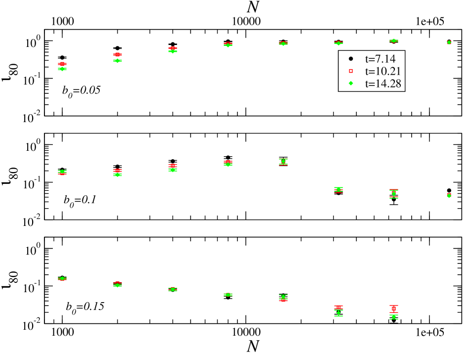
Figure 1: Each panel shows $\iota_{80}$ for a given $b_{0}$ as a function of $N$. In each case its value, averaged over an ensemble of realisations of Poissonian initial conditions (see footnote in text for details of number of realizations), is plotted at three different times, well after the virialisation of the system (at $t\approx 2$).

We have studied the evolution for many values of $b_{0}$ in the range between $0$ and $0.3$. Shown in Fig.  1 are results for the measured $\iota_{80}$ at three times as a function of $N$ three chosen values of the initial viral ratio $b_{0}$ ($b_{0}=0.05$, $b_{0}=0.1$ and $b_{0}=0.15$) and for Poissonian initial conditions. Each point is the average value calculated over $M$ of realisations of the given initial condition . The error bars indicate the estimated error on the mean.

As noted the system contracts to its minimal size at $t\approx 1$ and then re-expands and is already well virialized by $t\approx 2$. The results for the different times indicated (starting from $t\approx 7$) and plotted in Fig. 1 thus monitor the stability of the measured shape parameter $\iota_{80}$ at “long times”. A very strong stability of the result is in fact observed in all but the simulations at the lowest $N$ — with up to a couple of thousand particles — in the case $b_{0}=0.05$. Such an evolution at lower particle number — towards a more spherically symmetric structure — is, as has been studied in detail by Theis & Spurzem (1999) for similar initial conditions — due to two body collisionality. Beyond $N=4000$ such effects do not appear to play any role in the evolution on the time scales we simulate, and the values of $\iota_{80}$ obtained at a given $N$ are very stable in time.

Let us consider now the dependence on $N$ of these “final” $\iota_{80}$. Depending on the value of $b_{0}$, the plots show very different qualitative behaviours: for $b_{0}=0.05$ (upper panel) an apparently asymptotic value of $\iota_{80}\approx 1$ is reached at $N\approx 10^{4}$; for $b_{0}=0.15$ (lower panel) $\iota_{80}$ is always much smaller and appears to decrease monotonically to zero as $N$ increases to its largest value. We will see below that the value of $\iota_{80}$, even in the cases where it is very small, is always measurably larger than the initial value of $\iota_{80}$, i.e. the measured asymmetry, albeit small, is above the level of the intrinsic noise introduced by sampling the density field with a finite $N$. For the intermediate case, $b_{0}=0.1$ (middle panel), we see a very different behaviour, which is, very roughly, an interpolation, in a narrow range of $N$ just above $N=10^{4}$, between the other two cases: up to $N=16000$ the final $\iota_{80}$ grows up to an average value of $\iota_{80}\approx 0.4$, while at $N=32000$ it is about an order of magnitude smaller. In summary, in the first and last case the behaviours as a function of $N$ are apparently a simple monotonic convergence towards an asymptotic value which is already very well approximated for a few thousand particles. In the intermediate case such a convergence towards the asymptotic value is observed only when there is roughly an order of magnitude more particles.

What lies behind these very different behaviours, both quantitative and qualitative, are the physical differences between the non-linear dynamics in the different cases: for $b_{0}=0.05$ the system strongly breaks spherical symmetry, while at $b_{0}=0.15$ this is not the case. As discussed in the literature (see references above), this symmetry breaking is in principle due to so-called “radial orbit instability”: stationary spherically symmetric solutions of the collisionless Boltzmann equation are unstable when the velocity dispersion is purely, or strongly, radial as originally shown by Polyachenko (1981). Such an instability exists for some range of the parameter (or parameters) characterising the anisotropy of the velocity distribution, and is expected to correspond to an existence of the instability starting out of equilibrium at values of $b_{0}$ up to some critical value. The simplest interpretation of the behaviour in the case $b_{0}=0.1$ is then that this value is just above the critical value, but sufficiently close to it that the larger intrinsic fluctuations about spherical symmetry present at smaller $N$ can allow the system to access the instability. This behaviour can be considered to be an example of the sensitivity to finite size effects characteristic of critical phenomena.

The naive interpretation of these results is thus the following. Convergence (to within some chosen precision) to the continuum result is obtained in all cases with a sufficiently large $N$. This number may, however, be very significantly larger if the initial condition is close to a “critical” point where the final state obtained changes qualitatively. Unless one is very close to such a point, on the other hand, it appears that the only finite $N$ effect in a simulation one needs to worry about in this system is two body collisionality. We will see now that these conclusions are not valid when we study the temporal evolution carefully.

3.2 $N$ dependence of temporal evolution

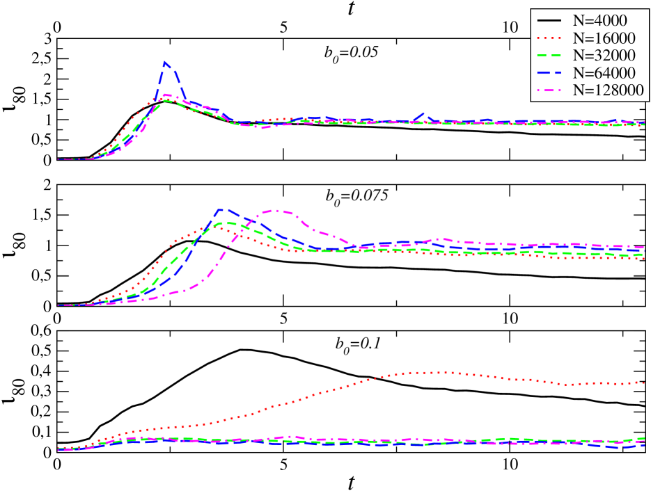
Figure 2: Each panel shows, for a given fixed value of $b_{0}$, the temporal evolution of $\iota_{80}$ as a function of time averaged over an ensemble of realisations with the indicated values of $N$. (The number of realisations in each case is the same as in the previous figure).

The above analysis relies on the study of the convergence of the macroscopic properties at relatively long times, well after the system has “settled down” to virial equilibrium. If we are only interested in the state of the system at asymptotically long times this is sufficient. However if, as for example in the context of cosmological simulations, the temporal evolution of macroscopic quantities needs to be resolved, convergence tests must be applied to these. Shown in Fig. 2 is the evolution of $\iota_{80}$ as a function of time, starting from realisations of our Poissonian initial conditions with the indicated values of $b_{0}$, for a range of different values of $N$. If we limit ourselves to examining the curves for $t>7$, our conclusions about convergence are those obtained above from Fig. 1: for a sufficiently large $N$ there appears to be clear convergence of the curves. However, considering now also times $t<7$ for the cases $b_{0}=0.05$ and $b_{0}=0.075$ (i.e. in which the final state breaks radial symmetry), the convergence is much poorer, or even apparently not attained at all: in particular the time at which the instability in $\iota_{80}$ develops in the case $b_{0}=0.075$ visibly depends on the number of particles, with the time at which $\iota_{80}$ attains its maximum shifted by almost two dynamical times between the largest two simulations. In the case $b_{0}=0.05$ the difference in this time is much smaller, but the details of the evolution around the maximum appears to be quite different. In either case it is clear that even at $N=128000$ one cannot conclude that the temporal macroscopic evolution has converged.

The shift of the time at which the instability in $\iota_{80}$ develops is explained simply making the hypothesis that the effective seeds for its development are the finite $N$ fluctuations in the initial conditions which break the spherical symmetry: as $N$ increases their amplitude is decreased, and thus their development retarded. This can be further tested by comparing evolution at given $N$ from our two different sets of initial conditions, Poissonian and lattice-like. Given that, at fixed $N$, the amplitude of the density fluctuations around perfect spherical symmetry are suppressed in the lattice initial conditions compared to those in the Poissonian initial conditions, the seeds for the instability are smaller. Thus, if our interpretation of the previous results is correct, we would anticipate that there should be a delay in the development of the instability at a given level. Shown in Fig. 3 are plots of the evolution of $\iota_{80}$ averaged over five realisations of the two cases, for two values of $b_{0}$ in the range where there is symmetry breaking, and also for the case $b_{0}=0.1$. In the first two cases, including the one corresponding to the upper panel in Fig.  2 in which the $N$ dependence of the temporal evolution was not so evident in this figure, we indeed see a clear delay in the onset of the instability for the lattice initial conditions. This is confirmed by Fig. 4 which shows the evolution at early times, in the time window $[0.5,1.5]$, for the individual realisations in each case. The lower panel in both figures show that, for the case $b_{0}=0.1$ where the final symmetry is very small, there is also a measurable relative delay of the development of the asymmetry which depends on the initial amplitude. As the evolution continues (see Fig. 3), however, the difference between the realisations appears to be more or less wiped out, in contrast in particular to the case $b_{0}=0.025$, in which the memory of the very subtle difference in the initial conditions appears clearly to persist up to the longest time simulated.

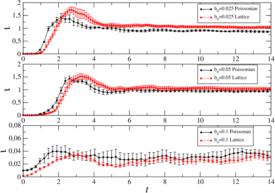
Figure 3: Each panel shows, for a given value of $b_{0}$, the mean temporal evolution of $\iota_{80}$, and its estimated error, in five realisations with $N=10^{5}$ particles of Poissonian (filled lines) and lattice (dashed line) initial conditions.

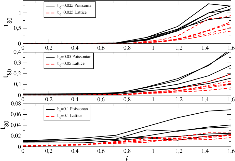
Figure 4: Evolution at early times ($0.5<t<1.5$) of $\iota_{80}$ in the five realisations of Poissonian (filled lines) and lattice (dashed line) initial conditions from which the averages in the previous figure are calculated.

The data we have shown up to now is averaged over a number of realisations of each initial condition. For most cases the dispersion between the single realisations is small once $N$ is greater than a few thousand. We have observed, however, that this is not always true: in cases where the evolution is very sensitive to the value of $N$, e.g., for $b_{0}=0.1$ around the transition observed between $N=10^{4}$ and $N=10^{5}$, there is also a very large dispersion between the different realisations. This is illustrated in Fig.  5 which shows the evolution in different realisations of the $b_{0}=0.1$ Poissonian initial condition with $N=16000$ particles. Remarkably we find that the macroscopic evolution can be completely different from realisation to realisation, i.e. the system manifests an apparent chaoticity of its macroscopic behaviour. We note that behaviour of this kind (“macroscopic stochasticity”) has been observed previously in N-body systems modelling galaxies by Sellwood & Debattista (2009). This kind of behaviour is incompatible with any even approximate convergence at this value of $N$, but it does not exclude convergence at significantly larger values of $N$. Indeed the apparent convergence at larger $N$ for this initial $b_{0}$ observed in Fig.  1 is associated with a very small dispersion in the results from realisation to realisation at larger $N$. As we have discussed in our case this highly fluctuating behaviour occurs in the region which appears to be stable for spherically symmetric equilibria, but very close to the unstable region. It is however also possible that it could be a marginally unstable region, for which a recent analysis of a long-range toy model (Barré et al., 2016) has shown that there can be a strong sensitivity of the evolution, and the final state, to the initial conditions (Barré et al., 2016). In either case what we observe is presumably the result of the competition between two different modes of instability around stationary solutions which are so close to one another that their finite $N$ samplings at the given $N$ can overlap, while at larger $N$ this will not be the case and a single mode of instability will dominate.

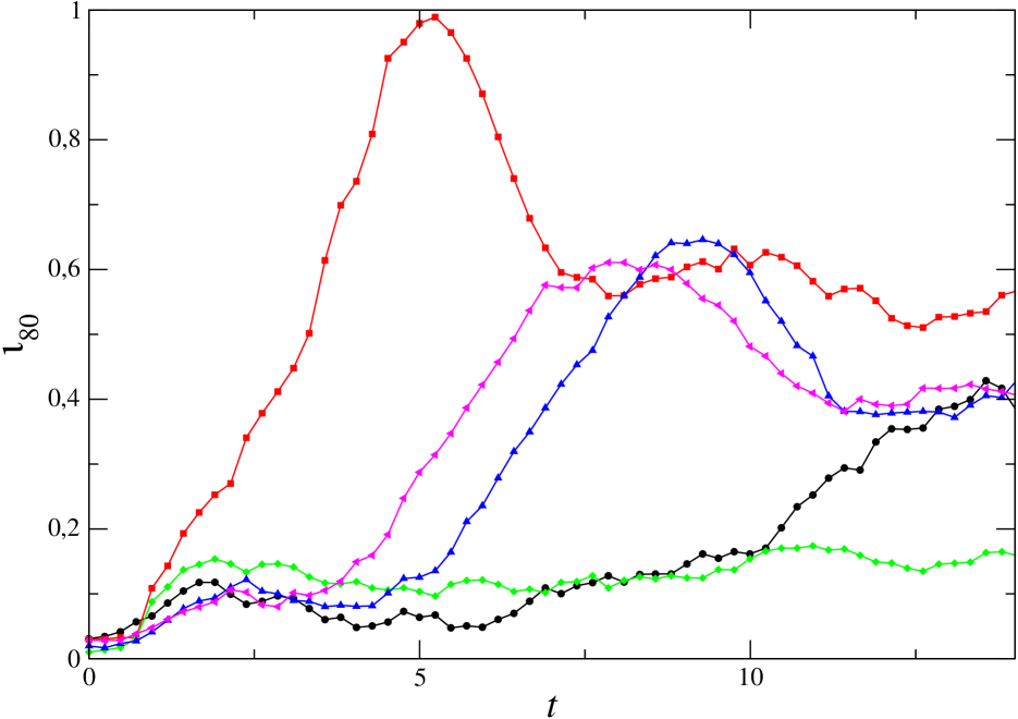
Figure 5: Temporal evolution of $\iota_{80}$ in different realisations with $N=16000$ of initial conditions with $b_{0}=0.1$.

4 Discussion and conclusions

The main motivation for this study is to understand better whether the results obtained with large N-body simulations of self-gravitating systems represent faithfully the evolution, up to some time, of a given collisionless system. Let us consider now carefully what our study allows us to conclude in this respect.

In a suite of N-body simulations at different $N$ of a simple class of initial conditions we have shown that the macroscopic evolution manifests two very different $N$ dependences. On the one hand, in our simulaions at smaller $N$ we have been able to observe that there is an $N$ dependence coming from two-body collisional effects. This is quite straightforward to identify in a numerical study as a clearly $N$ dependent drift of appropriately chosen macroscopic quantities, as observed previously in similar systems (e.g. Theis & Spurzem (1999)). On the other hand there is a distinct $N$ dependence associated with the presence of instabilities in the collisionless dynamics. This arises because the initial seeds for the instability themselves depend on $N$. This dependence on $N$ is in practice much more difficult to find, as it manifests itself only in a very weak dependence of the time of triggering of the instability, and not, at sufficiently large $N$, in the properties of the state to which the instability drives the system. Indeed despite the fact that these initial conditions have been studied fairly extensively in the literature, and that it might seem evident to expect that there may be such a dependence on $N$, this subtle dependence of the evolution on $N$ has apparently gone unnoticed, other than in a study by Boily & Athanassoula (2006). These authors remarked, for cold initial conditions characterized by a power law profile of density $\rho(r)\propto r^{-3/2}$, a very slow convergence with $N$ of parameters characterizing the shape of the final triaxial system obtained (similar to our $\iota_{80}$). Specifically they concluded from a detailed study analogous to ours in Section 3.1, that “$N=10^{5}$ or larger is required for convergence of axial aspect ratios” in numerical experiments of this type. In light of our analysis it is clear that this conclusion can be expected to depend strongly on the initial condition. Further it does not apply to the temporal evolution of the system. Indeed the latter should in fact be expected not to converge at all as $N$ is extrapolated, and indeed it is not evident even that final axis ratios should be expected to converge unless the instability leading to breaking of symmetry occurs well after virialisation. In the case analysed by Boily & Athanassoula (2006) this appears not to be the case, and in general for very cold initial conditions to reach such an asymptotic regime in a numerical study would appear to be a considerable challenge.

We emphasise again that while the first type of $N$ dependence is indicative of collisional effects, and therefore of effects which are absent in the collisionless limit which it is the goal to simulate, the second type of $N$ dependence is due to an instability which exists in the collisionless limit — indeed the radial orbit instability is an instability of stationary solutions of the collisionless Boltzmann equation. Thus the $N$ dependence observed in the convergence study we have performed does not mean that the N-body system does not approximate well the behaviour of a collisionless self-gravitating system. It just means that it does not follow the collisionless evolution of the exactly spherically symmetric initial condition to which the $N\rightarrow\infty$ limit considered converges. Instead when the instability develops, the N-body system is following evolution from an initial condition with a finite perturbation away from the exact spherical symmetry of the model initial condition. To test numerically whether this evolution is indeed collisionless one would need to perform a different large $N$ extrapolation of an N-body initial condition at some given $N=N_{0}$, in which $N$ is varied keeping the fluctuations away from spherical symmetry at $N_{0}$ fixed, i.e., one would need to resample at larger and larger $N$ the density field of the $N=N_{0}$ simulation. The suite of N-body simulations should then converge well at any finite time. The difficulty with such a convergence study is that such a resampling always introduces new fluctuations at smaller scales. One does not know a priori whether these fluctuations may play some significant role in the dynamics. We plan to study this issue further in future work.

Our study thus illustrates that, in performing a convergence study of an N-body self-gravitating system to test whether it can be considered to represent that of a collisionless system, there may be $N$ dependences which may be very much slower than those of two-body effects in particular, and consequently much more difficult to identify in a numerical study. Indeed a generic instability sourced by fluctuations, with amplitude of order $\frac{1}{\sqrt{N}}$ if sampling is Poissonian, will lead to a dependence of the time it develops at, which will grow in proportion to $\log N$ for an exponential instability (assuming that numerical integration is sufficiently accurate that numerical errors do not seed the instability). In the simple case we have chosen to study we have been able to find such an $N$ dependence because it is associated with a known instability, the role of which is easy to detect as it leads to a change in the symmetry of the structure. In the generic case where one does not know a priori that there are instabilities — and do not have evident tools for recognising that they may be present and playing a central role in the dynamics — one could thus easily miss completely in a numerical convergence study that the results are in fact $N$ dependent.

Although we have not analysed the specific case of cosmological simulations we believe our results are very relevant to them. In this respect the important point to note is that initial fluctuations of cosmological simulations, although known theoretically at all scales, are necessarily sampled in N-body simulations only at scales above the initial grid spacing (see e.g. Bertschinger (1998)). When an initially overdense region undergoes non-linear evolution the collapsing region is qualitatively similar to that of the finite system we have studied. The resulting collapsing structures typically contain a very modest number of particles. Indeed for typical cold dark matter initial conditions, such structure formation is hierarchical, proceeding through the collapse of successively larger structures starting from ones containing only a handful of particles. The fluctuations associated with the finite number of particles sampling any structure, which have no direct relation to those of the continuum model’s initial conditions, can then potentially play a crucial part in the non-linear evolution of the structure. Indeed, in respect of the particular example we have studied, we note that several works in the literature (Huss et al., 1999; MacMillan et al., 2006) find that the radial orbit instability apparently plays a crucial role in the evolution of cosmological halos, and even claim that it is this instability which explains the apparent “universality” of the profiles of cosmological halos. While existing convergence studies (see e.g. Power et al. (2003)) of such collapses appear to show that these profiles are in fact $N$ independent, we note that they involve the comparison of the “final” state of the halos rather than the detailed comparison of their temporal evolution. As we have seen here it is the latter which shows up the subtle $N$ dependences which would otherwise have escaped us. If radial orbit instability indeed plays a central role in the evolution of simulated cosmological halos, it is important to verify that the amplitude of the fluctuations driving the instability are not determined by the finite number of particles used to sample the initial conditions. More generally, in the strongly non-linear regime we should be very cautious in concluding that results truly represent the relevant continuum limit on the basis of convergence studies covering a very modest range of particle number. These issues could be addressed further in a controlled manner by using initial conditions more closely representative of those of collapsing regions in N-body cosmological simulations, and, for example, by studying the effect of additional external forces mimicking the tidal forces inevitably present in such a setting. Finally we note that our results provide also a strong motivation for the use of different methods to study collisionless systems, and in particular direct integration of the collisionless Boltzmann equation as attempted by some recent studies (Yoshikawa et al., 2013; Colombi et al., 2015; Sousbie & Colombi, 2016).

Numerical simulations have been run on the Cineca Fermi cluster (project VR-EXP HP10C4S98J), and on the HPC resources of The Institute for Scientific Computing and Simulation financed by Region Ile de France and the project Equip@Meso (reference ANR-10-EQPX- 29-01) overseen by the French National Research Agency (ANR) as part of the Investissements d’Avenir program. T.W. is supported by The Thailand Research Fund (TRF) under contract number TRG5880036.

References

- Aguilar & Merritt (1990) Aguilar L., Merritt D., 1990, Astrophys. J., 354, 73
- Antonov (1973) Antonov V. A., 1973, in Omarov T. B., ed., Dynamics of Galaxies and Star Clusters, p. 139–143
- Barnes et al. (2009) Barnes E. I., Lanzel P. A., Williams L. L. R., 2009, Astrophys. J., 704, 372
- Barré et al. (2016) Barré J., Métivier D., Yamaguchi Y. Y., 2016, Phys. Rev. E, 93, 042207
- Benhaiem & Sylos Labini (2015) Benhaiem D., Sylos Labini F., 2015, Mon.Not.Roy.Astron.Soc., 448, 2634
- Bertschinger (1998) Bertschinger E., 1998, Annu. Rev. Astron. Astrophys., 36, 599
- Binney & Tremaine (1994) Binney J., Tremaine S., 1994, Galactic Dynamics. Princeton University Press
- Boily & Athanassoula (2006) Boily C. M., Athanassoula E., 2006, Mon.Not.Roy.Astron.Soc., 369, 608
- Colombi et al. (2015) Colombi S., Sousbie T., Peirani S., Plum G., Suto Y., 2015, Mon.Not.Roy.Astron.Soc., 450, 3724
- Diemand et al. (2004) Diemand J., Moore B., Stadel J., Kazantzidis S., 2004, MNRAS, 348, 977
- El-Zant (2006) El-Zant A. A., 2006, Mon.Not.Roy.Astron.Soc., 370, 1247
- Gabrielli et al. (2010) Gabrielli A., Joyce M., Marcos B., 2010, Phy. Rev. Lett., 105, 210602
- Henon (1973) Henon M., 1973, Astron. Astrophys, 24, 229
- Huss et al. (1999) Huss A., Jain B., Steinmetz M., 1999, Astrophys. J., 517, 64
- Joyce & Marcos (2007) Joyce M., Marcos B., 2007, Phys. Rev., D76, 103505
- MacMillan et al. (2006) MacMillan J. D., Widrow L. M., Henriksen R. N., 2006, Astrophys. J., 653, 43
- Maréchal & Perez (2011) Maréchal L., Perez J., 2011, Transport Theory and Statistical Physics, 40, 425
- Merritt & Aguilar (1985) Merritt D., Aguilar L. A., 1985, Mon.Not.Roy.Astron.Soc., 217, 787
- Polyachenko (1981) Polyachenko V. L., 1981, Soviet Ast. Lett., 7, 79
- Power et al. (2003) Power C., Navarro J. F., Jenkins A., Frenk C. S., White S. D. M., Springel V., Stadel J., Quinn T., 2003, Mon.Not.Roy.Astron.Soc., 338, 14
- Roy & Perez (2004) Roy F., Perez J., 2004, Mon.Not.Roy.Astron.Soc., 348, 62
- Sellwood (2015) Sellwood J. A., 2015, Mon.Not.Roy.Astron.Soc., 453, 2919
- Sellwood & Debattista (2009) Sellwood J. A., Debattista V. P., 2009, Mon.Not.Roy.Astron.Soc., 398, 1279
- Sousbie & Colombi (2016) Sousbie T., Colombi S., 2016, Journal of Computational Physics, 321, 644
- Springel (2005) Springel V., 2005, Mon.Not.Roy.Astron.Soc., 364, 1105
- Sylos Labini et al. (2015) Sylos Labini F., Benhaiem D., Joyce M., 2015, Mon.Not.R.Astron.Soc., 449, 4458
- Theis & Spurzem (1999) Theis C., Spurzem R., 1999, Astron. Astrophys., 341, 361
- Yoshikawa et al. (2013) Yoshikawa K., Yoshida N., Umemura M., 2013, Astrophys. J., 762, 116