A textual transform of multivariate time-series for prognostics

Abstract

Prognostics or early detection of incipient faults is an important industrial challenge for condition-based and preventive maintenance. Physics-based approaches to modeling fault progression are infeasible due to multiple interacting components, uncontrolled environmental factors and observability constraints. Moreover, such approaches to prognostics do not generalize to new domains. Consequently, domain-agnostic data-driven machine learning approaches to prognostics are desirable. Damage progression is a path-dependent process and explicitly modeling the temporal patterns is critical for accurate estimation of both the current damage state and its progression leading to total failure. In this paper, we present a novel data-driven approach to prognostics that employs a novel textual representation of multivariate temporal sensor observations for predicting the future health state of the monitored equipment early in its life. This representation enables us to utilize well-understood concepts from text-mining for modeling, prediction and understanding distress patterns in a domain agnostic way. The approach has been deployed and successfully tested on large scale multivariate time-series data from commercial aircraft engines. We report experiments on well-known publicly available benchmark datasets and simulation datasets. The proposed approach is shown to be superior in terms of prediction accuracy, lead time to prediction and interpretability.

I Introduction

Industrial equipment such as aircraft engines, locomotives and gas turbines follow a conservative cadence of scheduled maintenance to insure equipment availability and safe operations. It is still common to have several unscheduled maintenance events that lead to unplanned downtime, loss of productivity and in some situations jeopardize public safety. Condition-based maintenance (CBM) can reduce maintenance cost while still providing safe operations. The primary goal of CBM is to track and predict equipment health using sensed measurements and operating conditions. The latter task of predicting the future health state and estimating remaining useful life falls under the umbrella of Prognostics. It has been estimated that the savings achieved from optimizing the use of engineering equipment can lead to up to $30B of savings in the aviation sector alone [1].

Observability into the degradation pattern of an equipment and likelihood estimate of fault at a future time can greatly improve availability, efficiency and safety of industrial equipments – costly maintenances can be held off until needed, and equipment load or usage can be adjusted based on current and predicted health status. However, accurate prognostics for complex engineering systems is challenging due to (1) interdependent components, (2) lack of full physical understanding of various failure modes and their effects on performance, and (3) accurate modeling of damage progression under uncertain operating conditions. While the nominal operating behavior of an engineering system can be modeled and controlled, modeling the response of a faulty equipment or component to operating conditions and control commands is challenging. In this regard, data-driven methods, particularly domain-agnostics ones, are a good alternative to create predictive models of system health.

While ubiquitous sensing and increased connectivity has given greater visibility into the behavioral changes of a machine as it ages, it has fueled a surge in massive time-series data from industrial and commercial equipment such as aircraft engines, gas turbines and home appliances. In this scenario, the task of modeling hidden health state in a data-driven manner becomes even harder as a large volume of temporal data needs to be ingested both during the learning and the real-time application phase. Moreover, during the application phase these models need to run on low footprint embedded processors to predict equipment health.

We propose a novel approach for early identification of industrial units with shorter life spans. Our approach works by transforming the multivariate temporal data into a sequence of tokenized symbols and utilizes popular off-the-shelf text-classification strategies for predictive modeling. Working a in a domain agnostic way, this approach provides a scalable solution for modeling temporal patterns in sensor data and predicting the future health state of an industrial equipment. We use real and simulation data-sets for equipment degradation to demonstrate our methodology. The system has been deployed and tested successfully on real multivariate time-series data from commercial jet engines acquired over 18 months. In the paper, to maintain confidentiality and reproducibility of our experiments, we use the popular aircraft engine degradation benchmark datasets provided by NASA [2] and degradation or phase-transition of a chaotic-oscillator [3]. Experiments show that our approach is able to capture the temporal dynamics of damage propagation to accurately predict the future health state of an equipment early in its life. We show that our approach is robust in the presence of significant noise, whereas well-known existing approaches, temporal as well as non-temporal, perform comparably only when the dataset is much cleaner.

Notation

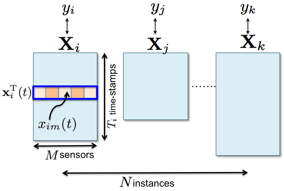
Figure 1: Time-series dataset notation

Let $\mathbf{x}_{i}(t)\in\mathbb{R}^{M}$ be the $M$-dimensional column vector of observations made at time $t$ for equipment $i$, with $x_{im}(t)$ as the value of the $m^{\text{th}}$ sensor at time $t$. Let $\mathbf{X}_{i}=[\mathbf{x}_{i}(1),\dots,\mathbf{x}_{i}(T_{i})]^{\prime}=(\mathbf{x}_{i})_{0}^{T_{i}}$ be a $M$-dimensional time-series data, where each row corresponds to a multivariate observation made at a particular time-stamp. Let the collection $\mathbb{X}=\{\mathbf{X}_{j}:1\leq j\leq N\}$ be the time-series dataset of $N$ instances. Let $\bm{y}=[y_{1},\dots,y_{N}]$, $y_{j}\in\{0,1\}$ be the set of outcomes or class labels e.g. $0\rightarrow$ healthy and $1\rightarrow$ faulty. Note that a time-series instance $\mathbf{X}_{i}\in\mathbb{R}^{T_{i}\times M}$ is generated by an equipment unit over time and is associated with the equipment unit’s label $y_{i}$; also time-series instances $\mathbf{X}_{i}$ can be of different lengths $T_{i}$, the dimensionality of the time-series $M$ is considered to be fixed across all instances.

II Our Approach

A typical textual document consists of a hierarchy of entities: characters, words, phrases, sentences, paragraphs, sections, chapters. We propose a textual transform to convert time-series data into a text document – where individual time stamped observations from each sensor can be thought of as characters, a sequence of characters desribing a temporal pattern will be words, and combination of such sequences will lead to phrases or sentences. Observations from one sensor will form a section of the document, leading to a multiple section document for multivariate data. In this way the entire time-series can be seen as an evolving journal in a textual sense.

The next few sections describe the specifics of enabling the textual representation discussed above. The overall work flow is presented in Figure 2.

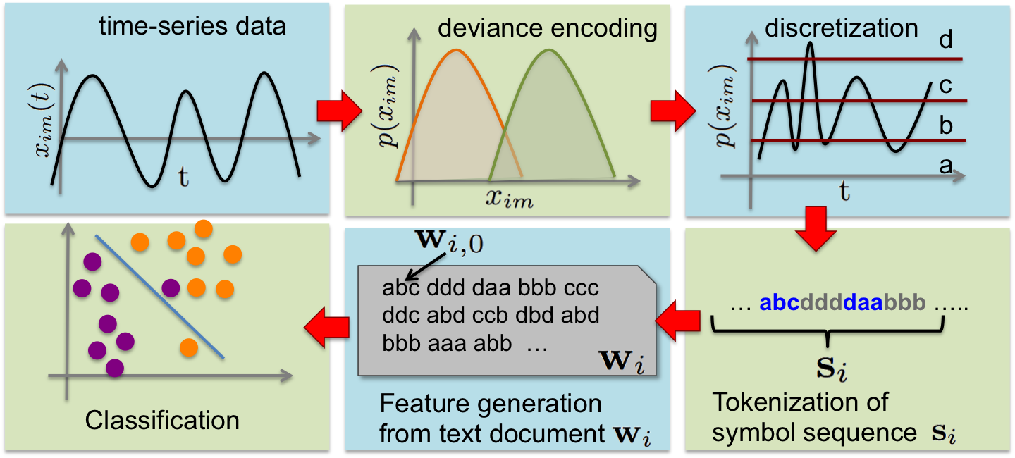
Figure 2: Process workflow for converting time-series to textual bag-of-words representation

II-A Encode abnormal behavior

In this work, we intend to discover signatures that are indicative of degrading or damaged equipment. If the general expected behavior of a healthy equipment is known a priori, then encoding the observations based on their alignment or deviation from the healthy state seems to be a reasonable choice. The healthy state operation of an equipment can either be derived from the physical or thermo-dynamical process governing the equipment, or it can be estimated in a completely data-driven way by acquiring historical records of operation in the healthy state. We choose the latter, more generic data-driven approach, since in many practical scenarios it may not be possible to completely describe a complex thermo-dynamical system with multiple interacting components in the context of changing and unknown or unrecorded environmental variables. Intuitively, we want to encode the observations by the likelihood of their occurrence with respect to a healthy unit. Formally, we need a map $f_{1}:\mathbb{R}^{M}\rightarrow\mathbb{R}$ that converts the observed series into a series of likelihoods $(\mathbf{x}_{i})_{0}^{T_{i}}\rightarrow(\Pr(\mathbf{x}_{i}))_{0}^{T_{i}}$. Depending on desired complexity of modeling the likelihood, one may choose a simple unimodal distribution (such as Gaussian), a mixture model such as Dirichlet process based Gaussian mixture model (DPGMM) [4], or more complex models. In this work, we choose among four approaches:

1. znorm-self: The data is centered and scaled per unit using the mean and variance of data from each unit.

2. znorm-all: The data is centered and scaled at the fleet-level using the mean and variance computed using data from all units.

3. DPGMM-univariate: A uni-modal Gaussian distribution may not explain different modes of operation. A univariate DPGMM is inferred over observations from each sensor across all units. Then, each observation for a sensor is encoded as the likelihood of its occurrence using the DPGMM model.

4. DPGMM-multivariate: A multivariate DPGMM is inferred over observations from all sensors from all units. Each multivariate observation is then encoded as the likelihood of its occurrence using the DPGMM.

II-B Discretize and Symbolize

Discretization of continuous features is a popular machine learning problem and several approaches have been studied in the past [5]. In this step, we map the real-valued series into a sequence of symbols. We define a mapping $f_{2}:\mathbb{R}\rightarrow\Phi$ that is a partition on the space $\mathbb{R}$, and each cell of the partition maps to the appropriate symbol in $\Phi$. Thus the original series $(\mathbf{x}_{i})_{0}^{T_{i}}$ gets converted into a string $\mathbf{s}_{i}\in\Phi^{T_{i}}$, such that $\mathbf{s}_{i}=(f_{2}(\mathbf{x}_{i}(j)):0\leq j\leq T_{i})$, with length same as the original time series $|\mathbf{s}_{i}|=T_{i}$.

We study two approaches for discretization: (a) Maximum Entropy Partition (MEP) [6] splits the data-space into $|\Phi|$ equiprobable regions. Popular for time series discretization [7, 8], it creates finer partitions in data-rich regions and coarser in partitions where data is less frequent in an unsupervised manner; (b) Recursive Minimal Entropy Partitioning (RMEP) [9] is a supervised approach to create partitions with minimum class entropy. Here we use encoded values from step 1 (section II-A) for all units, and label all data from a unit with it’s final classification label. Using this dataset $\mathbb{D}=\{(x,y):x\in\mathbf{x}_{i},y=y_{i},1\leq i\leq N\}$, we discover threshold $\theta$ that splits the instances into sets $\mathbb{D}_{0}$ and $\mathbb{D}_{1}$, such that class information entropy $H(\mathbb{D},\theta)$ is minimized.

$$H(\mathbb{D},\theta) = \frac{|\mathbb{D}_{0}|}{|\mathbb{D}|}H(\mathbb{D}_{0})+\frac{|\mathbb{D}_{1}|}{|\mathbb{D}|}H(\mathbb{D}_{1})$$

$$H(\mathbb{D}_{j}) = -\sum_{r\in\{0,1\}}\Pr(C_{r},\mathbb{D}_{j})\log\Pr(C_{r},\mathbb{D}_{j})$$

$$\Pr(C_{r},\mathbb{D}_{j}) = \frac{|\{(x,y):(x,y)\in\mathbb{D}_{j}\wedge y=C_{r}\}|}{|\mathbb{D}_{j}|}$$

Threshold discovery is applied recursively using a stopping criteria based on the Minimal Description Length Principle, thereby achieving multiple bins for discretization.

II-C Tokenize

Tokenization is the step of splitting long sequences into constituent tokens/words. Thus, we wish to split the symbolic sequence $\mathbf{s}_{i}$ into constituent tokens $\mathbf{w}_{i}=(\mathbf{w}_{i,0},\ldots,\mathbf{w}_{i,K_{i}})$, such that $\mathbf{s}_{i}=\mathbf{w}_{i,0}\frown\ldots\frown\mathbf{w}_{i,K_{i}}$, and $K_{i}\ll T_{i}$. , where $\frown$ is the string concatenation operator. In most natural languages, tokenization is enabled by punctuation or morphology. However, tokenizing a symbolized time-series is an open challenge. The simplest approach involves generating tokens of fixed lengths $L$, where token length $L$ is found via cross-validation.

As an alternative approach to determine $L$, we consider the symbol sequence as a Markov Chain over $|\Phi|$ symbols, with order $L$. The order is the number of past symbols that a future symbol depends on, or, $\Pr(\mathbf{s}_{i,m}|\mathbf{s}_{i,m-1},\ldots,\mathbf{s}_{i,0})=\Pr(\mathbf{s}_{i,m}|\mathbf{s}_{i,m-1},\ldots,\mathbf{s}_{i,m-L})$. We use the Conditional Mutual Information (CMI) based approach to estimate $L$ [10]. This method has been shown to be demonstrably better than previously well known approaches based on Bayesian information criterion (BIC), Akaike Information criterion (AIC), the Peres-Shields estimator or the ones based on the $\phi$-divergences [10]. In the CMI-based approach the goal is to find the smallest $L$ such that

$$I_{c}(L+1)=I(\mathbf{s}_{i,m};\mathbf{s}_{i,m-L}|\mathbf{s}_{i,m-1},\ldots,\mathbf{s}_{i,m-L+1})=0$$

where $I_{c}(L+1)$ is the conditional mutual information between observations that are $L$ time steps apart. Once estimated, $L$ is used as the token-length.

II-D Generate features

With the tokenization step, we have transformed the original time-series into a sequence of punctuated symbol sequences akin to words in a text document. This representation lets us leverage the popular bag-of-words representation that is successful in the text-mining domain. In this approach, each document is represented as a vector of term weights. The vector magnitudes represent a score for every word in the document. For our model, we use the popular TF-IDF (Term Frequency - Inverted Document Frequency) score, specifically the variant commonly known as ltc. The vocabulary is defined as the union of all the tokens resulting from all the time-series, $\mathbb{V}=\{w|w\in\mathbf{w}_{i},1\leq i\leq N\}$. If $\#(j|\mathbf{w})$ denotes the number of occurrences of the token $j$ in the textual transform $\mathbf{w}_{i}$ of time-series $(\mathbf{x}_{i})_{0}^{T_{i}}$, then the ltc scores can be calculated as follows:

$$\mathbf{w}_{i} \rightarrow \mathbf{b}_{i}:=\frac{[b_{1},\ldots,b_{|\mathbb{V}|}]}{\|[b_{1},\ldots,b_{|\mathbb{V}|}]\|}$$

$$b_{j} = \log(\#(j|\mathbf{w}_{i})+1)\log\frac{|N|}{|\{\mathbf{w_{k}}:\exists j\in\mathbf{w_{k}},\mathbf{w_{k}}\in\{\mathbf{w}_{1},\ldots,\mathbf{w}_{N}\}\}|}$$

where each $b_{j}$ is the score for a token in the textual transform

II-E Classify

Given the bag-of-words representation achieved in the previous step, now it is straightforward to apply any popular text-classification algorithm for learning a model that distinguishes between healthy and unhealthy units. We choose the linear kernel based Support Vector Machine (SVM), a very popular and successful model for text classification.

II-F Computational Complexity

In Table I, we list the computational complexity of the major components of the textual transform process. The transformation procedure, in its simplest form, by choosing the fastest approach at each step, is linearly dependent on the size of the dataset, making it highly practical for large-scale deployment. Since the steps involve mere iterations over the dataset, this is highly amenable to big-data systems based on map-reduce that are highly popular among industrial monitoring systems. Even with the most expensive choice of approach at each step, the algorithm does not suffer significantly since it is still linear in the number of instances and the length of the time-series, possibly the largest variables for practical prognostics deployment.

Encode	Discretize	Tokenize
Gaussian: $\mathcal{O}(NMT)$	MEP: $\mathcal{O}(NMT)$	Fixed-length: $\mathcal{O}(NMT)$
DP-GMM [11]: $\begin{cases}&\text{(covariance)}\\ \mathcal{O}(NMT),&\text{diagonal}\\ \mathcal{O}(NM^{2}T),&\text{tied}\\ \mathcal{O}(NM^{3}T),&\text{full}\end{cases}$	RMEP:$\mathcal{O}(MNT\log(NT))$ [12]	Markov Order: $\mathcal{O}(NMT)$

TABLE I: Computational Complexity of the major steps in the textual transformation process. $T:=\text{max}_{i}T_{i}$. Typically, $M\ll N$ and $M\ll T$. For avoiding notation clutter, we have ignored several quantities that linearly (or sublinearly) affect the complexities, but are insignificant in magnitude compared to $N,M,T$. These include, among others, the number of mixture components for DPGMM, the number of splits for RMEP, or the number of candidate lengths tested for Markov Chain order estimation.

III Data sets

The proposed methods have been deployed on proprietary datasets from commercial aircraft engines. To maintain confidentiality, while still retaining reproducibility of the results, the experiments in this paper are presented on 4 similar public benchmark datasets and simulated datasets with multiple levels of signal to noise ratio.

III-A Real aircraft engine dataset

This proprietary dataset consists of data from $59$ aircraft engines of which $20$ engines are distressed or known to have usage-based equipment underperformance. The other $39$ engines are known to be in a healthy state. The determination of healthy and distressed engines is based on detailed manual inspections that are cumbersome and time consuming, hence the need for automatic detection of distressed engines. Each flight, or cycle of operation, of an engine generates a row of data for that engine detailing the sensor values measured at certain critical phases of operation such as flight takeoff. We used multivariate measurements from 10 chosen sensors for $18$ months of usage for each of the chosen engines. In this timeframe, each engine has flown about $650-1560$ times, leading to a dataset with approximately half a million sensor observations.

III-B C-MAPSS Turbofan dataset

These datasets, created and publicly released by the NASA Prognostics Center of Excellence, consist of run-to-failure observations of aircraft gas turbine engines using the C-MAPSS tool-kit [2].

The gas turbine engine system consists of five major rotating components – fan (F), low pressure compressor (LPC), high pressure compressor (HPC), high pressure turbine (HPT), and low pressure turbine (LPT), as seen in Figure 3. Deterioration $D$ of the engine is modeled as a loss of flow and loss of efficiency of the HPC module. Starting from a randomly chosen initial state, deterioration rate $\dot{D}$ is modeled as an exponential rate of change for both modes of failures.

Figure 3: Schematic of a Turbofan engine [2]

Four datasets are available, with data for 100, 100, 249 and 260 engines in each set respectively. Each dataset corresponds to a certain mode of damage propagation under different conditions. For each engine, 21 sensor measurements and 3 operating parameters are recorded for every cycle of engine operation. Six different operating conditions determined by altitude, Mach number and throttle resolver angle are present. Lifespans of engines are in the range 128-525 cycles.

Figure 4 depicts the distribution of life-expectancies of the units, in terms of number of flights, in the four datasets.

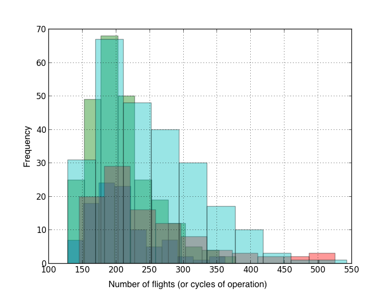
Figure 4: Distribution of the life expectancies of units in the four C-MAPSS datasets

We use these datasets for the task of identifying engines that have lower life expectancy. We have split engines in each datasets into two classes based on whether they have higher or lower than median lifespan in that dataset, leading to roughly balanced classes. This is a realistic industrial setting where identification of units with lower than usual life expectancy allows timely root-cause analysis, increased monitoring, preventive maintenance and operational adaptations. As the detection of under-performance needs to happen early in life, we use observations only from the initial 50 cycles of operation for training and testing splits.

III-C Duffing oscillator dataset

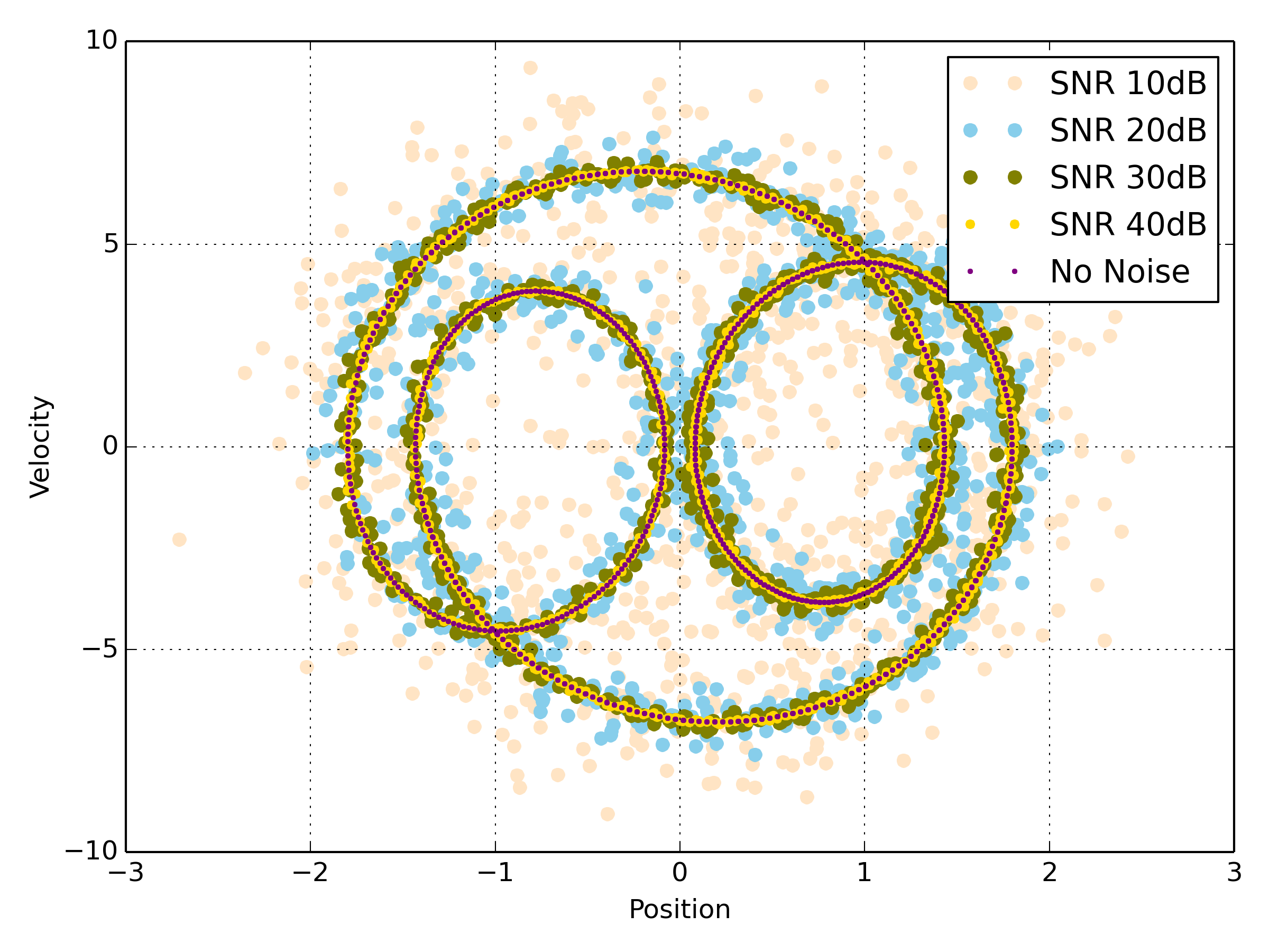
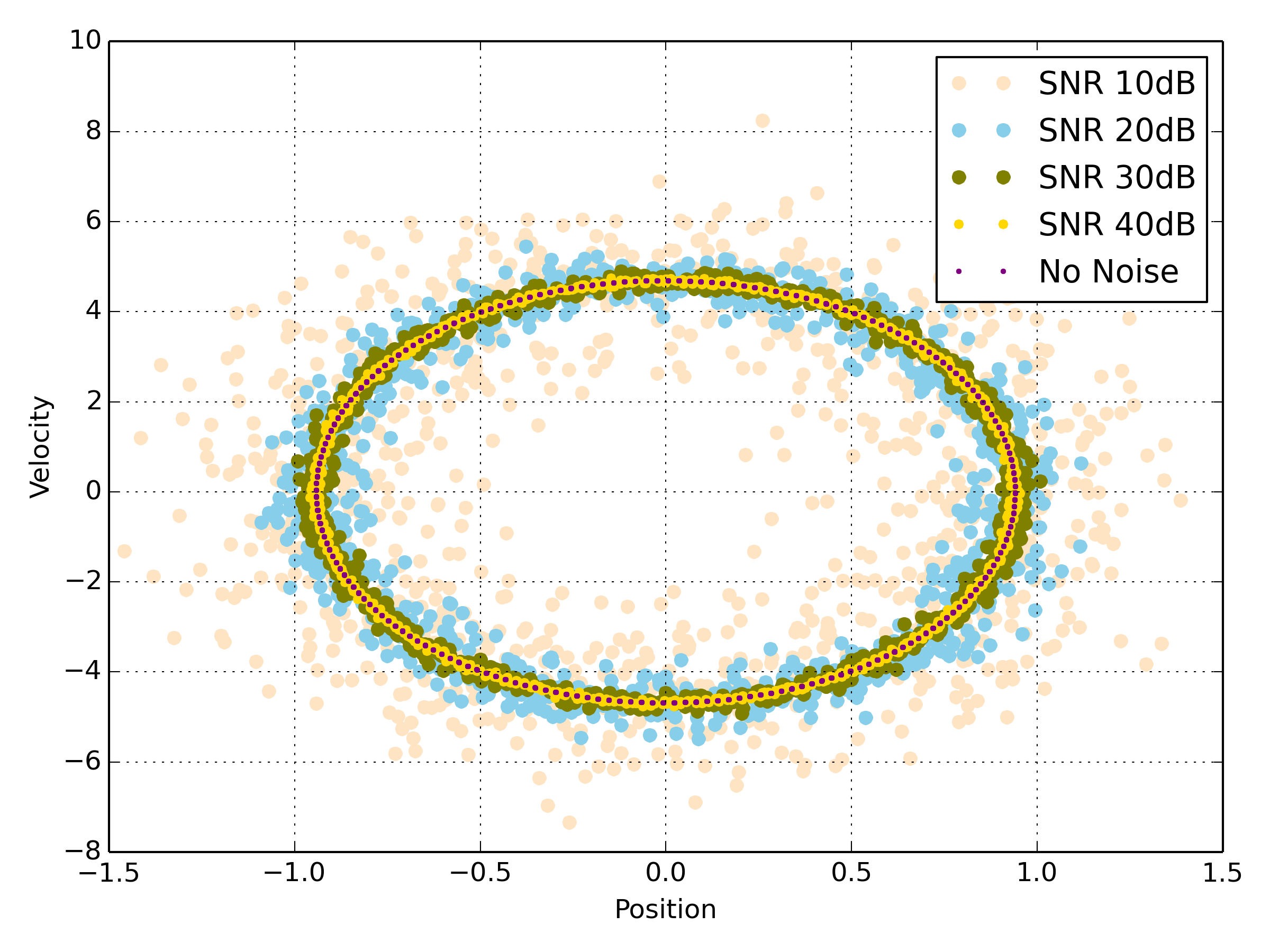
(a)	(b)	(c)

Figure 5: Phase plot of the duffing oscillator for various noise levels (a) $\nu(t_{s})=0.29$, (b) $\nu$ distribution used for creating two classes, and (c) phase plot for $\nu(t_{s})=0.325$

Another set of data is generated using the Duffing Oscillator which is described by the following second order non-autonomous system:

$$\frac{d^{2}x(t)}{dt^{2}}+\nu(t_{s})\frac{dx(t)}{dt}+\kappa x(t)+\alpha x^{3}(t)=A\cos(\Omega_{f}t)$$ (1)

The system dynamics evolve in the time-scale of the time parameter $t$ while the quasi-static dissipation parameter $\nu(t_{s})$ changes slowly in time $t_{s}$. This system describes the motion of a damped oscillator across a twin well potential function. This equation has been used as the underlying model for many engineering systems such as those for electronic circuits, structural vibrations and chemical bonds [3] . This system shows a slow change in dynamics as the parameter $\nu(t_{s})$ is increased with an abrupt change of behavior or a phase change for $\nu(t_{s})>0.3$. This behavior is analogous to fault propagation in engineering systems where slow changes in system parameters such as component efficiency or corrosive damage leads them from nominal to anomalous and finally to an abrupt failed state. The parameter $\nu(t_{s})$ can be thought of as the health parameter which is typically unobserved or not measured. The goal is to infer the health state of the system using only its observations – position and velocity in this case.

Duffing data for classification experiments, is generated by solving the Duffing equation for different values of $\nu(t_{s})$ which are sampled from a bimodal Gaussian distribution with means $0.290$ (healthy) and $0.325$ (faulty) and a common standard deviation of $0.00625$; parameter $A=22.0$, $\Omega_{f}=5.0$, $\kappa=1.0$ and $\alpha=1.0$ with an initial condition of $[0.0,\ 0.1]^{\prime}$. The scipy package for Python is used to solve equation 1 using runge-kutta method of order (4)5 using a time-step of $\Delta_{t}=T_{f}/200$, and then down-sampled to create $\approx 200$ time-steps long time-series data for position and velocity for each value of $\nu(t_{s})$; here $T_{f}=2*\pi/\Omega_{f}$ is the time-period of the forcing function. Four data-sets consisting of $500$ samples each of healthy and faulty are used is created with four levels of signal-to-noise ratio (SNR) – 10dB, 20 dB, 30 dB, 40 dB and clean.

IV Experiments

IV-A Experimental Setup

We developed our system in Python and used the scikit-learn library of algorithms. All the results reported have been estimated using nested cross-validation. That means, the outer cross-validation averages performances over multiple training-testing splits, and the inner cross-validation is done for model-selection/parameter-tuning over multiple training-validation splits. For the inner model-selection loop and outer accuracy estimation, we perform 10-fold cross-validation [13]. For the support vector machines we chose the hinge-loss or margin-penalty parameter, commonly denoted as $C$, from the set $\{10^{-2},\ldots,10^{2}\}$.

IV-B Classification Experiments

We use both non-temporal and temporal state-of-the-art algorithms as baselines for comparison with the proposed method:

• Non-temporal: In this setting, we use data from last $k$ cycles and label them with the final classification label of each unit, leading to $k$ labeled instances. We use this data to train an SVM and call this approach SVM-final (SVM-F). In addition to the final instances, we use the initial few cycles from each unit and label those as the healthy class, as all units were healthy in the beginning. We call this approach SVM initial-final (SVM-IF). We have also tried using all the data from each unit and labeling them with the final classification label, but the performance was significantly worse as all units are healthy initially. We also use RandomForest classifiers instead of SVM to get additional non-temporal baselines RF-F and RF-IF. The parameter $k$ was tuned via cross-validation.

• Temporal: Here we treat the problem as time-series classification (TSC) and use 1-Nearest Neighbor classifier with DTWCV – Dynamic Time Warping metric with wraping window set by cross-validation, for classification. Our choice is motivated by a comprehensive evaluation of TSC algorithms that says that “a new algorithm for TSC is only of interest to the data mining community if it can significantly outperform DTWCV” [14]. We call this approach NNDTW.

Our approach called TTC (for Textual Time-series enCoding) and its variants are summarized in Table II

Deviance Encoding	Discretization	Tokenizaton
S: znorm-self	M: MEP	E: Equilength
A: znorm-all	R: RMEP	M: Markov
U: DP-GMM univariate
M: DP-GMM multivariate

TABLE II: Quick reference for the naming convention used on the TTC configurations. Each configuration is a 3-letter acronym based on the strategy utilized for each of the three steps. For example, TTC-SME means the znorm-self(S) was used for encoding deviance, MEP(M) was used for discretization and Equilength(E) tokens were used for the tokenization step

Table III provides the results of the classification experiments. The textual-transform based models, TTC-*, clearly outperform other approaches with a significant margin. The superior performance over non-temporal approaches indicate that there is much to be gained by utilizing the temporal nature of the observations from each unit, especially in the case of C-MAPSS dataset and the noisy versions of the Duffing dataset.

The performance of the strong TSC baseline, DTWCV, is particularly weak, suggesting that this problem is not a typical TSC problem. Since engines are operated independently, controlled differently, behave in idiosyncratic ways, and observations are typically noisy, there is not much to be gained by directly comparing the shapes of their time-series profiles, a common underlying theme of TSC algorithms, particularly of the DTWCV. A unique aspect of sensor time-series from engineering systems is fixed rate sampling for data collection. In this scenario, warping the time-axis for DTW calculation can lead to creation of artifacts not intrinsic to the original shape or pattern. This might also explain the poor performance of the proven baseline NNDTW in this study. The performance of DTWCV improves on the duffing dataset as the signal to noise ratio (SNR) improves. However, practical scenarios rarely lead to clean observations.

On the other hand, TTC approaches benefit from aggregating the common occurrences through the bag-of-words representation and thereby simulating a cumulative damage model of the engine. Thus, if an engine has a high occurrence of mishandling, or rough weather, the model will be able to aggregate those through term-frequency and weigh them appropriately using the frequency of their occurrence through the population (inverse document frequency). The SVM classifier at the end of the TTC steps would then weigh the damage precursors highly to learn a superior model for prognostics.

Method	Jet Engines	C-MAPSS Dataset				Duffing Dataset
	1	1	2	3	4	10dB	20dB	30dB	40dB	clean
MF	0.660	0.506	0.506	0.506	0.500	0.500	0.500	0.500	0.500	0.500
RF-F	0.730	0.478	0.533	0.663	0.671	0.675	0.790	0.864	0.981	0.998
RF-IF	0.710	0.536	0.506	0.506	0.565	0.621	0.809	0.859	0.980	0.999
SVM-F	0.660	0.528	0.533	0.506	0.654	0.638	0.819	0.823	0.819	0.831
SVM-IF	0.560	0.528	0.486	0.506	0.626	0.621	0.712	0.711	0.819	0.831
NNDTW	0.730	0.526	0.568	0.523	0.500	0.752	0.839	0.987	0.999	0.999
TTC-SME	0.793★	0.637	0.618	0.606	0.455	0.892	0.992★	0.995	0.998	0.997
TTC-SMM	0.793★	0.688★	0.525	0.667	0.473	0.852	0.983	0.998	0.998	0.999
TTC-SRE	0.727	0.546	0.495	0.564	0.516	0.852	0.984	0.993	0.999	0.999
TTC-SRM	0.677	0.574	0.494	0.614	0.500	0.841	0.983	0.991	0.997	0.997
TTC-AME	0.710	0.578	0.634★	0.726	0.714★	0.894★	0.985	0.999★	1.000★	0.998
TTC-AMM	0.740	0.619	0.529	0.726	0.553	0.861	0.989	0.999★	1.000★	0.998
TTC-ARE	0.593	0.537	0.595	0.727★	0.674	0.883	0.987	0.993	0.998	0.999
TTC-ARM	0.660	0.578	0.617	0.727★	0.600	0.882	0.985	0.993	0.998	0.999
TTC-UME	0.727	0.567	0.572	0.618	0.502	0.825	0.949	0.997	0.996	0.999
TTC-UMM	0.760	0.423	0.479	0.426	0.550	0.837	0.959	0.998	0.999	0.999
TTC-URE	0.707	0.504	0.603	0.526	0.516	0.726	0.881	0.987	0.984	0.999
TTC-URM	0.657	0.524	0.482	0.507	0.530	0.589	0.828	0.991	0.937	0.999
TTC-MME	0.643	0.506	0.533	0.506	0.465	0.807	0.886	0.980	0.999	0.997
TTC-MMM	0.710	0.506	0.478	0.506	0.500	0.764	0.840	0.979	0.998	1.000★
TTC-MRE	0.543	0.494	0.537	0.494	0.470	0.754	0.819	0.886	0.998	0.966
TTC-MRM	0.443	0.494	0.482	0.494	0.500	0.500	0.503	0.760	0.959	0.765
TTC-overall	0.793	0.666	0.595	0.737	0.726	0.869	0.983	0.997	0.996	0.997

TABLE III: Accuracy of the classification approaches. The best performance for each dataset is indicated by a ^★. Refer to Table II for acronyms of TTC-variants. TTC-overall is an all-encompassing approach that is tuned over all the TTC-* approaches using only the training set to select the best one and then predict over the test set, for each train-test split

IV-C Early detection

In this section, we compare the performance of candidate algorithms in detect units with low life expectancy early in their life. For this experiment, we trained all algorithms using initial $150$ cycles of units in the training set, and evaluated prediction accuracy of the trained model on the test set as a function of increasing number of cycles observed from the test units. Figure 6 depicts the performance trend as a function of the increasing number of cycles for the test set. The results have been averaged over 10-fold cross-validation. It can be observed that our approach is significantly better than the baselines in the initial stages. The baselines, especially RF-F and RF-IF, achieve comparable performance as more information from the test unit becomes available. However, it is too late.

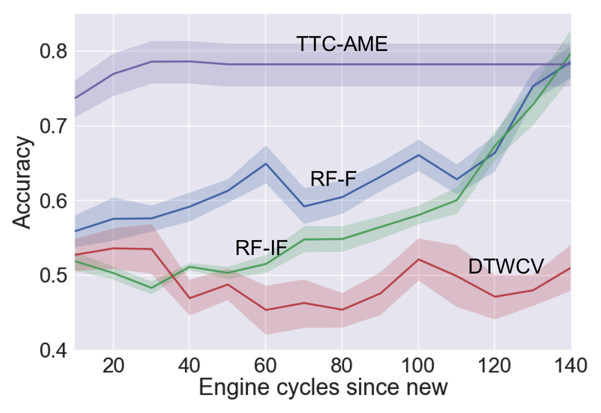
Figure 6: Comparison of the trend of accuracy as a function of the number of initial observations from a unit on the dataset C-MAPSS 4

IV-D Analyzing the textual transform

Words in natural language documents have been commonly desrcibed by the power-law distribution. Being long-tailed, it has a few very common stop words, and many infrequent rare words. The stop-words, being common to all documents, do not provide distinguishability, while rare words do not generalize to larger corpus. Consequently, the middle-class of the power-law distribution is critical to good predictive performance. In our problem, few discrete symbols ($1\leq|\Phi|\leq 3$), with short word lengths ($L\leq 3$) leads to too many stop-words, since shorter sequences of small number of symbols are likely to be observed very commonly in the time-series, thereby leading to low discrimination among different behaviors. On the other hand, many discrete symbols ($|\Phi|\geq 15$), with long word-lengths ($L\geq 10$), leads to many rare words, thereby making it infeasible to get good generalizable performance. This trend of accuracy with respect to the symbol size and token length is evident in the Figure 7. From the Figure 7, it can be observed that the optimal performance occurs at alphabet-size $|\Phi|=10$ and token length $L=4$ and the performance tapers down around this.

Figure 7: Effect of word-length $L$ and alphabet-size $|\Phi|$ on classification accuracy for dataset Duffing SNR 20dB. Colors denote levels of accuracy, see colorbar

As an alternative approach for determining token length, we had suggested that the symbolic time-series may be modeled as a Markov Chain and its order may be estimated. From our experiments, we observe that the order of the Markov Chain representing the symbolic time-series comprising of 10 symbols is about 4 for the Duffing dataset with SNR 20dB. Thus, every symbol sequence of 4 consecutive observations contains sufficient history that’s predictive of the future symbol to come. This aligns well with our empirical assessment that the optimal word-length for symbol size 10 is indeed around 4, as seen in Figure 7.

IV-E Interpretability

Another aspect of the proposed approach is the interpretability of results. Using feature weights it is possible to identify the words (or features) that were most useful for discriminating between the two classes. These words, or sequences of symbols, can be mapped back to the original dataset, thus identifying time-series subsequences that were important for classification. Figure 8 shows as a colormap the weights for important words identified by TTC for classification of healthy and faulty classes; feature weights depicted are for words constructed from the symbols of velocity data. It can be seen in subfigure (a) that for healthy class (the negative class), important segments with large negative weight are around the transition points – locations where the phase-space plot diverges away to form the inner loops. Similarly, subfigure (b) shows for the faulty class (the positive class) the time segments associated with important words with large positive weights. With a similar approach, for the case of real aircraft engine, we were able to discover words that when mapped back to the time-series data helped the domain experts understand the earliest signatures of impending distress.

(a)	(b)

Figure 8: Feature weights of words formed using velocity sensor data for Duffing dataset with SNR 20dB shown as color map; weights are shown for the AME variant of proposed TTC approach. Subfigure (a) shows large negative weights for healthy or the negative class, and subfigure (b) shows large positive feature weights for the faulty or the positive class; critical segments such as transition points into inner loop formation in the negative class are correctly selected by the approach

IV-F Identifying groups of units to monitor

A key goal of prognostics is to enable efficient resource allocation for preventive maintenance. After the initial 3 steps of encoding, discretization and tokenization to get the textual transform, any well-known text clustering algorithm can be used on the transformed data containing unit-as-a-document to segment the fleet of units by their behavior. Figure 9 depicts pairwise cosine-similarity matrix of units transformed into documents. The appearance of block-matrices along the diagonal demonstrates that typically units with similar life-expectancies have similar textual profiles.

Figure 9: Pairwise cosine similarity between textual transforms for units in the dataset C-MAPSS1.Pairwise-similarities above the 75 percentile threshold have been shown in black. The textual transform was based only on the first 200 cycles for each unit

V Related Work

The work in the area of prognostics and health management (PHM) can be divided into three broad categories based on the time-horizon of predictions and prior knowledge of faults or degradation. Anomaly detection deals with detecting any unusual changes in system chararteristics when the true cause of these changes may not be known a priori or even understood. This approach is good and applicable for new product lines whose degradation patterns may not be fully understood, and also to monitor old and more studied systems to detect unknown patterns and events. These approaches typically employ unsupervised learning approaches to model the nominal or healthy behavior and then flag systems deviating with respect to the nominal. The output from an anomaly detection module can be used to trigger the next stage of PHM for further investigation. The area of anomaly detection is not limited to PHM and it has been applied in various domains, a summary of which appears in [15], and  [16], while a review of anomaly detection for discrete sequences can be found in [17]

Fault detection & Diagnostics (FDD) involves prior knowledge of faults under consideration known instances or physical understanding of its effect on performance. The goal is to build models that can detect the presence of these faults and categorize them. For equipment health management, when the effects of a fault are well understood or when physically modeling the system nominal behavior is feasible, physics-based approaches can be employed to help detect and determine the root-cause of the fault. Supervised data-driven approaches are used when the physics of failure is too complex to model or not well understood. Good overall reviews of FDD can be found in [18]. The prediction time horizon for anomaly detection and fault detection & diagnostics is typically very short or current and they are used to determine the current state of the system under consideration.

Prognostics deals with forecasting equipment health state. This problem is characteristically different from the previous two in terms of the predicting time horizon and modeling of the temporal patterns of equipments characteristics become imperative. Both model-based and data-driven approaches have been used for this purpose. Model-based approaches such as particle filtering [19] make use of system-dynamics and fault propagation model to estimate the health state of the system in the future. Data-driven approaches on the other hand look to model the observed temporality due to system and fault dynamics with minimal information. Review of prognostics methodologies for rotating machines like an aircraft engines, batteries can be found in found in [20, 21]

Numerous discrete representations have been proposed for mining time series data. A detailed discussion on discretizing real-valued data appears in  [5], and [22] summarizes approaches specific to discretizing real-valued time-series data. Some of these approaches, such as Discrete Wavelet Transform (DWT) [23], Discrete Fourier Transform (DFT) [24], Piecewise Linear/Constant models such as Piecewise Aggregate Approximation (PAA) [25, 26] or APCA [27] and Singular Value Decomposition (SVD) [26], offer real-valued representations that are not amenable to the textual transformation that we wish to achieve. The symbolic representation known as SAX (Symbolic Aggregate approXimation) [8] is one approach suitable for our need of generating text documents. SAX and its variants are widely accepted as being suitable for common time-series mining tasks such as clustering [28], classification [29], indexing [30], summarization [31], rare event detection [32].

V-A Key contributions

Although bag-of-words strategy for time-series has been explored before [33, 34], in these approaches, the time-series is first tokenized into fixed length subsequences and then converted into the corresponding SAX representation. A tf-idf model is applied and 1-nearest neighbor classifier is used with cosine similarity as the distance metric. These approaches have been developed for univariate problems while ours is a multi-variate setting. Moreover, a distance metric based approach cannot filter irrelevant information. A regularized discriminative classifier such as a SVM or implicit feature selection using Random Forest is crucial for good performance. The deviance encoding step is also absent in these approaches, but it is very valuable for prognostics for encoding deterioration from normal. Also, tokenization used in these approaches is fixed length, while we offer an additional perspective of treating the time-series as a Markov chain for token length estimation.

The focus of our approach is structural similarity of time-series data, which is more relevant for discriminating dynamical patterns from engineering systems, as opposed to shape similarity which has been primary focus of previous works such as SAX-based approaches. Also, by utilizing mixture of Gaussians in the deviance encoding step, we facilitate the discovery of multi-mode operation of industrial equipments. This is unlike previous works that assume unimodality. We present a supervised alternative (RMEP) for symbolization to leverage class labels to achieve more discriminative symbolization as opposed to unsupervised approaches like SAX.

Our approach of utilizing a symbolic bag-of-words representation is novel for the prognostics application. Moreover, the analogy of time-series as a journal of observations from an industrial unit is a new perspective of formulating the prognostics problem. This transformation enables leveraging significant advances in scalability in text mining for prognostics and other time-series analyses. Unlike most other approaches in prognostics that are domain-specific, our methodology is data-driven allowing for a wider application base.

Much of the recent research in scalability for big-data analysis has happened in the domain of text-mining and linear models that can be learnt via Stochastic Gradient Descent. Our transformation of the multivariate time-series into a textual form enables the field of prognostics to benefit from the recent advances in scalability and big-data analysis of textual data.

VI Conclusions and Future Work

We demonstrated a novel approach to transform multivariate time-series data into a symbolic textual form that can directly leverage latest research in text mining, for scalability, interpretability and predictive performance. To this end, we have demonstrated successful use cases that solve well known problems in prognostics using off-the shelf text mining algorithms for classification. In addition to accurately classifying industrial units based on their life expectancy, the proposed approach can detect under-performance much earlier. Moreover, the proposed approach is generic and domain-agnostic allowing for a wider deployment.

Several directions are open for future exploration: (a) Integrated strategies for alphabet size and token length selection, (b) framework to allow incorporation of relevant domain knowledge if necessary, and (c) effect of token order, e.g. n-grams, on predictive performance

References

- [1] P. C. Evans and M. Annunziata, “Industrial internert: Pushing the boundaries of minds and machines,” 2012. [Online]. Available: http://www.ge.com/docs/chapters/Industrial_Internet.pdf
- [2] A. Saxena, K. Goebel, D. Simon, and N. Eklund, “Damage propagation modeling for aircraft engine run-to-failure simulation,” in Prognostics and Health Management, 2008. PHM 2008. International Conference on, Oct 2008, pp. 1–9.
- [3] V. L. Berdichevsky, Thermodynamics of Chaos and Order. Essex, England: Addison Wesley Longman, 1997.
- [4] C. E. Antoniak, “Mixtures of dirichlet processes with applications to bayesian nonparametric problems,” Ann. Statist., vol. 2, no. 6, pp. 1152–1174, 11 1974. [Online]. Available: http://dx.doi.org/10.1214/aos/1176342871
- [5] S. Garcia, J. Luengo, J. A. Saez, V. Lopez, and F. Herrera, “A survey of discretization techniques: Taxonomy and empirical analysis in supervised learning,” IEEE Trans. on Knowl. and Data Eng., vol. 25, no. 4, pp. 734–750, Apr. 2013. [Online]. Available: http://dx.doi.org/10.1109/TKDE.2012.35
- [6] A. Ray, “Symbolic dynamic analysis of complex systems for anomaly detection,” Signal Process., vol. 84, no. 7, pp. 1115–1130, Jul. 2004. [Online]. Available: http://dx.doi.org/10.1016/j.sigpro.2004.03.011
- [7] A. Apostolico, M. E. Bock, and S. Lonardi, “Monotony of surprise and large-scale quest for unusual words,” in Proceedings of the sixth annual international conference on Computational biology, ser. RECOMB ’02. New York, NY, USA: ACM, 2002, pp. 22–31. [Online]. Available: http://doi.acm.org/10.1145/565196.565200
- [8] J. Lin, E. Keogh, S. Lonardi, and B. Chiu, “A symbolic representation of time series, with implications for streaming algorithms,” in Proceedings of the 8th ACM SIGMOD workshop on Research issues in data mining and knowledge discovery, ser. DMKD ’03. New York, NY, USA: ACM, 2003, pp. 2–11. [Online]. Available: http://doi.acm.org/10.1145/882082.882086
- [9] U. M. Fayyad and K. B. Irani, “Multi-interval discretization of continuous-valued attributes for classification learning.” in IJCAI, 1993, pp. 1022–1029. [Online]. Available: http://dblp.uni-trier.de/db/conf/ijcai/ijcai93.html#FayyadI93
- [10] M. Papapetrou and D. Kugiumtzis, “Markov chain order estimation with conditional mutual information,” CoRR, vol. abs/1301.0148, 2013. [Online]. Available: http://dblp.uni-trier.de/db/journals/corr/corr1301.html#abs-1301-0148
- [11] D. M. Blei and M. I. Jordan, “Variational inference for dirichlet process mixtures,” Bayesian Analysis, vol. 1, pp. 121–144, 2005.
- [12] R. Kohavi and M. Sahami, “Error-Based and Entropy-Based discretization of continuous features,” in Proceedings of the Second International Conference on Knowledge Discovery and Data Mining, 1996, pp. 114–119. [Online]. Available: http://citeseerx.ist.psu.edu/viewdoc/summary?doi=10.1.1.47.5132
- [13] R. Kohavi, “A study of cross-validation and bootstrap for accuracy estimation and model selection,” in Proceedings of the 14th international joint conference on Artificial intelligence - Volume 2, ser. IJCAI’95. San Francisco, CA, USA: Morgan Kaufmann Publishers Inc., 1995, pp. 1137–1143. [Online]. Available: http://dl.acm.org/citation.cfm?id=1643031.1643047
- [14] J. Lines and A. Bagnall, “Ensembles of elastic distance measures for time series classification.” in SDM, 2014, pp. 524–532.
- [15] V. Chandola, A. Banerjee, and V. Kumar, “Anomaly detection: A survey,” ACM Comput. Surv., vol. 41, no. 3, pp. 15:1–15:58, Jul. 2009. [Online]. Available: http://doi.acm.org/10.1145/1541880.1541882
- [16] M. A. Pimentel, D. A. Clifton, L. Clifton, and L. Tarassenko, “A review of novelty detection,” Signal Processing, vol. 99, no. 0, pp. 215 – 249, 2014. [Online]. Available: http://www.sciencedirect.com/science/article/pii/S016516841300515X
- [17] V. Chandola, A. Banerjee, and V. Kumar, “Anomaly detection for discrete sequences: A survey,” Knowledge and Data Engineering, IEEE Transactions on, vol. 24, no. 5, pp. 823–839, May 2012.
- [18] V. Venkatasubramanian, R. Rengaswamy, K. Yin, and S. N. Kavuri, “A review of process fault detection and diagnosis: Part i: Quantitative model-based methods,” Computers & Chemical Engineering, vol. 27, no. 3, pp. 293 – 311, 2003. [Online]. Available: http://www.sciencedirect.com/science/article/pii/S0098135402001606
- [19] A. Marcos, S. Ganguli, and G. J. Balas, “An application of H- fault detection and isolation to a transport aircraft,” Control Engineering Practice, vol. 13, no. 1, pp. 105 – 119, 2005. [Online]. Available: http://www.sciencedirect.com/science/article/pii/S0967066104000425
- [20] J. Lee, F. Wu, W. Zhao, M. Ghaffari, L. Liao, and D. Siegel, “Prognostics and health management design for rotary machinery systems–reviews, methodology and applications,” Mechanical Systems and Signal Processing, vol. 42, no. 1-2, pp. 314 – 334, 2014. [Online]. Available: http://www.sciencedirect.com/science/article/pii/S0888327013002860
- [21] B. Saha, K. Goebel, S. Poll, and J. Christophersen, “Prognostics methods for battery health monitoring using a bayesian framework,” Instrumentation and Measurement, IEEE Transactions on, vol. 58, no. 2, pp. 291–296, Feb 2009.
- [22] J. Lin, E. Keogh, L. Wei, and S. Lonardi, “Experiencing sax: a novel symbolic representation of time series,” Data Min. Knowl. Discov., vol. 15, no. 2, pp. 107–144, Oct. 2007. [Online]. Available: http://dx.doi.org/10.1007/s10618-007-0064-z
- [23] K.-P. Chan and A.-C. Fu, “Efficient time series matching by wavelets,” in Proceedings of the 15th International Conference on Data Engineering, ser. ICDE ’99. Washington, DC, USA: IEEE Computer Society, 1999, pp. 126–. [Online]. Available: http://dl.acm.org/citation.cfm?id=846218.847201
- [24] C. Faloutsos, M. Ranganathan, and Y. Manolopoulos, “Fast subsequence matching in time-series databases,” in Proceedings of the 1994 ACM SIGMOD international conference on Management of data, ser. SIGMOD ’94. New York, NY, USA: ACM, 1994, pp. 419–429. [Online]. Available: http://doi.acm.org/10.1145/191839.191925
- [25] B.-K. Yi and C. Faloutsos, “Fast time sequence indexing for arbitrary lp norms,” in Proceedings of the 26th International Conference on Very Large Data Bases, ser. VLDB ’00. San Francisco, CA, USA: Morgan Kaufmann Publishers Inc., 2000, pp. 385–394. [Online]. Available: http://dl.acm.org/citation.cfm?id=645926.671689
- [26] K. Chakrabarti, E. Keogh, S. Mehrotra, and M. Pazzani, “Locally adaptive dimensionality reduction for indexing large time series databases,” ACM Trans. Database Syst., vol. 27, no. 2, pp. 188–228, Jun. 2002. [Online]. Available: http://doi.acm.org/10.1145/568518.568520
- [27] P. Geurts, “Pattern extraction for time series classification,” in Proceedings of the 5th European Conference on Principles of Data Mining and Knowledge Discovery, ser. PKDD ’01. London, UK, UK: Springer-Verlag, 2001, pp. 115–127. [Online]. Available: http://dl.acm.org/citation.cfm?id=645805.670003
- [28] C. Ratanamahatana, E. Keogh, A. J. Bagnall, and S. Lonardi, “A novel bit level time series representation with implication of similarity search and clustering,” in Proceedings of the 9th Pacific-Asia conference on Advances in Knowledge Discovery and Data Mining, ser. PAKDD’05. Berlin, Heidelberg: Springer-Verlag, 2005, pp. 771–777. [Online]. Available: http://dx.doi.org/10.1007/11430919_90
- [29] P. Siirtola, H. Koskimäki, V. Huikari, P. Laurinen, and J. Röning, “Improving the classification accuracy of streaming data using sax similarity features,” Pattern Recogn. Lett., vol. 32, no. 13, pp. 1659–1668, oct 2011. [Online]. Available: http://dx.doi.org/10.1016/j.patrec.2011.06.025
- [30] J. Shieh and E. Keogh, “isax: indexing and mining terabyte sized time series,” in Proceedings of the 14th ACM SIGKDD international conference on Knowledge discovery and data mining, ser. KDD ’08. New York, NY, USA: ACM, 2008, pp. 623–631. [Online]. Available: http://doi.acm.org/10.1145/1401890.1401966
- [31] N. Kumar, V. Lolla, E. Keogh, C. A. Ratanamahatana, and H. Van Herle, “A practical tool for visualizing and data mining medical time series,” in Proceedings of the 18th IEEE Symposium on Computer-Based Medical Systems, ser. CBMS ’05. Washington, DC, USA: IEEE Computer Society, 2005, pp. 341–346. [Online]. Available: http://dx.doi.org/10.1109/CBMS.2005.17
- [32] E. Keogh, J. Lin, and A. Fu, “Hot sax: Efficiently finding the most unusual time series subsequence,” in Proceedings of the Fifth IEEE International Conference on Data Mining, ser. ICDM ’05. Washington, DC, USA: IEEE Computer Society, 2005, pp. 226–233. [Online]. Available: http://dx.doi.org/10.1109/ICDM.2005.79
- [33] J. Lin, R. Khade, and Y. Li, “Rotation-invariant similarity in time series using bag-of-patterns representation,” J. Intell. Inf. Syst., vol. 39, no. 2, pp. 287–315, Oct. 2012. [Online]. Available: http://dx.doi.org/10.1007/s10844-012-0196-5
- [34] P. Senin and S. Malinchik, “Sax-vsm: Interpretable time series classification using sax and vector space model,” in Data Mining (ICDM), 2013 IEEE 13th International Conference on, Dec 2013, pp. 1175–1180.