The interstellar medium in [OIII]-selected star-forming galaxies at $z\sim 3.2$

Abstract

We present new results from near-infrared spectroscopy with Keck/MOSFIRE of [Oiii]-selected galaxies at $z\sim 3.2$. With our $H$ and $K$-band spectra, we investigate the interstellar medium (ISM) conditions, such as ionization states and gas metallicities. [Oiii] emitters at $z\sim 3.2$ show a typical gas metallicity of $\mathrm{12+log(O/H)=8.07\pm 0.07}$ at $\mathrm{log(M_{*}/M_{\odot})\sim 9.0-9.2}$ and $\mathrm{12+log(O/H)=8.31\pm 0.04}$ at $\mathrm{log(M_{*}/M_{\odot})\sim 9.7-10.2}$ when using the empirical calibration method. We compare the [Oiii] emitters at $z\sim 3.2$ with UV-selected galaxies and Ly$\alpha$ emitters at the same epoch and find that the [Oiii]-based selection does not appear to show any systematic bias in the selection of star-forming galaxies. Moreover, comparing with star-forming galaxies at $z\sim 2$ from literature, our samples show similar ionization parameters and gas metallicities as those obtained by the previous studies using the same calibration method. We find no strong redshift evolution in the ISM conditions between $z\sim 3.2$ and $z\sim 2$. Considering that the star formation rates at a fixed stellar mass also do not significantly change between the two epochs, our results support the idea that the stellar mass is the primary quantity to describe the evolutionary stages of individual galaxies at $z>2$.

1 Introduction

Recent near-infrared (NIR) spectroscopic surveys have suggested that star-forming galaxies at high redshifts ($z>1$) typically have different interstellar medium (ISM) conditions from those found in local star-forming galaxies (e.g. Masters et al., 2014; Steidel et al., 2014; Hayashi et al., 2015; Shapley et al., 2015; Holden et al., 2016; Kashino et al., 2017). Star-forming galaxies at high redshifts show a systematic offset from local galaxies on the Baldwin-Phillips-Terlevich diagram (so called BPT diagram; Baldwin et al. 1981; Veilleux & Osterbrock 1987), i.e. they have higher [Oiii]/H$\beta$ ratios with respect to [Nii]/H$\alpha$ (e.g. Erb et al., 2006a; Masters et al., 2014; Steidel et al., 2014; Shapley et al., 2015; Kashino et al., 2017). Also on a stellar mass versus [Oiii]/H$\beta$ ratio diagram (Mass–Excitation diagram; Juneau et al. 2011), star-forming galaxies at high redshifts show systematically higher [Oiii]/H$\beta$ ratios than local ones at a fixed stellar mass (e.g. Cullen et al., 2014; Shimakawa et al., 2015a; Holden et al., 2016; Strom et al., 2017; Kashino et al., 2017). These differences suggest that ISM conditions at high redshifts are different as a result of lower gas metallicities, higher ionization parameters, harder spectra of ionizing sources, and the combination of all these factors (e.g. Kewley et al., 2013; Nakajima & Ouchi, 2014; Steidel et al., 2014, 2016; Trainor et al., 2016; Strom et al., 2017; Kashino et al., 2017).

The relation between stellar mass and gas metallicity of star-forming galaxies has been investigated by several studies. It has been known that there is a positive correlation between stellar mass and gas metallicity since about 40 years ago (Lequeux et al., 1979). Now the stellar mass–gas metallicity relation is observed for star-forming galaxies from $z=0$ even up to $z\sim 5$ (Tremonti et al., 2004; Erb et al., 2006a; Maiolino et al., 2008; Mannucci et al., 2009; Henry et al., 2013; Stott et al., 2013; Cullen et al., 2014; Steidel et al., 2014; Troncoso et al., 2014; Wuyts et al., 2014; Yabe et al., 2015; Zahid et al., 2014; Sanders et al., 2015; Faisst et al., 2016; Onodera et al., 2016), and star-forming galaxies at higher redshifts have lower gas metallicities than local star-forming galaxies at a fixed stellar mass.

When estimating the gas metallicities of star-forming galaxies, the strong line methods are often used. The relations between strong emission line ratios and gas metallicities are obtained empirically using local star-forming galaxies (e.g. Pettini & Pagel 2004; Maiolino et al. 2008; Curti et al. 2017, and at $z=0.8$ by Jones et al. 2015) or with the photoionization models (e.g. Kewley & Dopita, 2002). It has been suggested that, however, the locally calibrated relations are no longer applicable to star-forming galaxies at high redshifts because the typical ISM conditions of star-forming galaxies seem to change from $z=0$ to higher redshifts (e.g. Kewley et al., 2013; Nakajima & Ouchi, 2014; Steidel et al., 2014; Kashino et al., 2017). It is still under discussion whether we can adopt the locally calibrated methods to star-forming galaxies at higher redshifts because some studies have reported that the physical conditions of Hii regions do not evolve with redshifts at a fixed metallicity (e.g. Jones et al., 2015; Sanders et al., 2016a). Moreover, it is known that the gas metallicities calibrated with different emission line ratios show systematic offsets from one another (Kewley & Ellison, 2008).

Studies of the ISM conditions and the mass–metallicity relation mainly target star-forming galaxies at $z<$ 2–2.5, up to the highest peak of galaxy formation and evolution (e.g. Hopkins & Beacom, 2006; Madau & Dickinson, 2014; Khostovan et al., 2015). However, the epoch of $z>3$ is also important because the cosmological inflow is likely to be prominent at this epoch (e.g. Mannucci et al., 2009; Cresci et al., 2010; Troncoso et al., 2014). The gas-phase metallicity of a galaxy reflects the relative contributions from star formation, gas outflow and gas inflow. Therefore, the metal content of galaxies is one of the key quantities in order to reveal how the gas inflow/outflow processes, as well as star formation, have an impact on galaxy formation and evolution.

NIR spectroscopic observations of star-forming galaxies at $z>3$ have been carried out by targeting UV-selected galaxies, such as Lyman break galaxies (LBGs) and Ly$\alpha$ emitters (LAEs; e.g. Steidel et al., 1996, 2003; Maiolino et al., 2008; Mannucci et al., 2009; Troncoso et al., 2014; Holden et al., 2016; Onodera et al., 2016; Nakajima et al., 2016). However, the evolution of the ISM conditions and the mass–metallicity relation especially at $z>3$ has not yet been fully understood because of the large uncertainties related to the estimation of gas metallicities and the limited sample sizes at this epoch (e.g. Onodera et al., 2016). Additionally, at $z>3$, it is difficult to obtain a representative sample of star-forming galaxies because available indicators of star-forming galaxies are limited. Since the UV-selected galaxies tend to be biased towards less dusty galaxies (Oteo et al., 2015), it is important to obtain a sample of star-forming galaxies using other selection techniques, which are less affected by dust extinction than the UV light. Rest-frame optical emission lines are very useful for this purpose.

There are some methods to select galaxies based on the strength of emission lines. The grism spectroscopy at the $H$-band by the Hubble Space Telescope (HST) can pick up galaxies at $z\sim$1–3 with strong emission lines in the rest-frame optical (e.g. Momcheva et al., 2016). Maseda et al. (2013, 2014) selected extreme emission line galaxies at $z\sim$1-2 based on the emission line flux and equivalent width from the HST NIR grism spectroscopy. Their sample consists of low mass galaxies of $\rm log(M_{*}/M_{\odot})\sim 8-9$. They showed that the extreme emission line galaxies are in the starburst phase with high specific star-formation rates (SFRs) and have high [Oiii]/H$\beta$ ratios ($\geq 5$). Hagen et al. (2016) also used the HST NIR grism data to construct a sample of the optical emission line-selected galaxies at $z\sim 2$. Comparing the sample with LAEs at similar redshifts, they found that the two galaxy populations have similar physical quantities in a stellar mass range of $\rm log(M_{*}/M_{\odot})\sim 7.5-10.5$.

Imaging observations with a narrow-band (NB) filter are also a very efficient way of constructing a sample of emission line galaxies in a particular narrow redshift slice (e.g. Bunker et al., 1995; Teplitz et al., 1999; Moorwood et al., 2000; Geach et al., 2008; Sobral et al., 2013; Tadaki et al., 2013). At $z>3$, the H$\alpha$ emission line, which is one of the most reliable tracers of star-forming galaxies, is no longer accessible from the ground. We need to use other emission lines at shorter wavelengths, such as [Oiii], H$\beta$, and [Oii] (Khostovan et al., 2015, 2016). As mentioned above, normal star-forming galaxies at high redshifts tend to show brighter [Oiii] emission lines. While there is a clear trend of decreasing [Oiii]/H$\beta$ ratio with increasing stellar mass (Juneau et al., 2011, 2014; Strom et al., 2017), the [Oiii] emission lines would be observable even for massive star-forming galaxies at $z>3$ because they are bright in [Oiii] intrinsically.

Is the [Oiii] emission line a useful tracer of star-forming galaxies at higher redshifts actually? Suzuki et al. (2015) have found that the [Oiii]-selected galaxies at $z>3$ show a positive correlation between stellar mass and SFR, which is known as the “main-sequence” of star-forming galaxies (e.g. Whitaker et al., 2012; Kashino et al., 2013; Tomczak et al., 2016). This suggests that we can trace the typical star-forming galaxies at $z>3$ using the [Oiii] emission line. Moreover, Suzuki et al. (2016) have shown that the [Oiii]-selected galaxies show similar distributions of stellar mass, SFR, and dust extinction as those of normal H$\alpha$-selected star-forming galaxies at $z\sim 2.2$, supporting the idea that the [Oiii] emission line can be used as a tracer of star-forming galaxies at high redshifts. Therefore, the [Oiii]-selected galaxies can probe dustier star-forming galaxies which are likely to be missed by the UV-based or [Oii] selection (Hayashi et al., 2013). We also note that another great advantages of NB-selected galaxies is the high efficiency of follow-up observations because their line fluxes and redshifts are obtained in advance by the NB imaging observations.

In this paper, we present the results obtained from the spectroscopic observation of [Oiii] emitters at $z=3.24$ in the COSMOS field obtained by the HiZELS survey (Geach et al., 2008; Sobral et al., 2009, 2013; Best et al., 2013; Khostovan et al., 2015). We carried out $H$ and $K$-band spectroscopy of the [Oiii] emitters with Keck/MOSFIRE. We investigate the physical conditions of the [Oiii] emitters at $z>3$ such as their ionization states and gas metallicities.

This paper is organized as follows: in Section 2, we present our parent sample of [Oiii] emitters at $z\sim 3.2$. We also describe our NIR spectroscopy of the [Oiii] emitters with Keck/MOSFIRE, and the details of the observations and data reduction/analyses. In Section 3, we show our results about the ISM conditions of our sample, and compare with other galaxy populations at the same epoch. In Section 4, we discuss the evolution of star-forming activities and ISM conditions of star-forming galaxies between $z\sim 3.2$ and $z\sim 2.2$. Finally we summarize this work in Section 5.

Throughout this paper, we assume the cosmological parameters of $\Omega_{\mathrm{m}}=0.3$, $\Omega_{\mathrm{\Lambda}}=0.7$, and $H_{\mathrm{0}}=70\ \mathrm{km\ s^{-1}Mpc^{-1}}$. All the magnitudes are given in AB system, and we adopt the Chabrier initial mass function (IMF; Chabrier 2003) unless otherwise noted. We refer to wavelengths of all emission lines using vacuum wavelengths.

2 Sample selection, observations, and reduction

2.1 Selection of [OIII] candidate emitters at $z\sim 3.24$

HiZELS (the High-$z$ Emission Line Survey; Sobral et al. 2012, 2013, see also Best et al. 2013) is a systematic NB imaging survey using NB filters in the $J$, $H$, and $K$-bands of the Wide Field CAMera (WFCAM; Casali et al. 2007) on the United Kingdom Infrared Telescope (UKIRT), and the NB921 filter of the Suprime-Cam (Miyazaki et al., 2002) on the Subaru Telescope. Emission line galaxy samples used in this study are based on the HiZELS catalogue in the Cosmological Evolution Survey (COSMOS; Scoville et al. 2007) field.

With the $\mathrm{H_{2}S1}$ filter (hereafter ${\rm NB}_{K}$  $\lambda_{\mathrm{c}}=2.121\ \mu\mathrm{m}$, and $\mathrm{FWHM=210\ \AA}$) of WFCAM, HiZELS selects the [Oiii]$\lambda$5008 emission from galaxies at $z=3.235\pm 0.021$. Here we construct a catalog of [Oiii] emitters at $z\sim 3.24$ by combining the ${\rm NB}_{K}$ emitter catalog from HiZELS (Sobral et al., 2013) and the latest photometric catalog in the COSMOS field (COSMOS2015; Laigle et al. 2016) in a similar way to Khostovan et al. (2015). The COSMOS2015 catalog includes the new deep NIR and IR data from UltraVISTA-DR2 survey and from the SPLASH (Spitzer Large Area Survey with Hyper-Suprime-Cam) project (Laigle et al., 2016). Such deep IR photometry becomes more important when estimating photometric redshifts and stellar masses of galaxies at higher redshifts.

In the first place, we search for counterparts of the ${\rm NB}_{K}$ emitters in the COSMOS2015 catalog with a searching radius of $0^{\prime\prime}.6$. The selection of the NB emitters are based on the color excess of NB with respect to broad band (BB), and the equivalent width. A parameter $\Sigma$ is introduced to quantify the significance of a NB excess relative to 1$\sigma$ photometric error (Bunker et al., 1995). This parameter $\Sigma$ is represented as a function of NB magnitude as follows (Sobral et al., 2013):

$$\Sigma=\frac{1-10^{-0.4(K-{\rm{NB})}}}{10^{-0.4({\rm ZP-NB})}\sqrt{\pi r^{2}_{\rm ap}(\sigma^{2}_{\rm NB}+\sigma^{2}_{K})}},$$ (1)

where NB and BB are NB and BB magnitudes, ZP is the zero-point of the NB (the BB images are scaled to have the same ZP as the NB images), $r_{\mathrm{ap}}$ is the aperture radius in pixel, and $\sigma_{\mathrm{NB}}$ and $\sigma_{\mathrm{BB}}$ are the rms per pixel of the NB and BB images, respectively (Sobral et al., 2013). Emission line fluxes, $F_{\mathrm{line}}$, and the rest-frame equivalent widths, $\mathrm{EW_{rest}}$, are calculated with

$$F_{\mathrm{line}}=\Delta_{\mathrm{NB}}\frac{f_{\mathrm{NB}}-f_{\mathrm{BB}}}{1-\Delta_{\mathrm{NB}}/\Delta_{\mathrm{BB}}},$$ (2)

and

$$\mathrm{EW_{rest}}=\Delta_{\mathrm{NB}}\frac{f_{\mathrm{NB}}-f_{\mathrm{BB}}}{f_{\mathrm{BB}}-f_{\mathrm{NB}}(\Delta_{\mathrm{NB}}/\Delta_{\mathrm{BB}})},$$ (3)

where $f_{\mathrm{NB}}$ and $f_{\mathrm{BB}}$ are the flux densities for NB and BB, and $\Delta_{\mathrm{NB}}$ and $\Delta_{\mathrm{BB}}$ are the FWHMs of the NB and BB filters, respectively (e.g. Tadaki et al., 2013). The selection criteria of the NB emitters are $\Sigma>3$ and the observed-frame equivalent-width of $\mathrm{EW_{obs}}\geq 80.8\ \AA$ (the rest-frame EW $\sim$ 19 Å for [Oiii] at $z=$3.24, Sobral et al. 2013; Khostovan et al. 2015). We select [Oiii] candidate emitters at $z\sim 3.24$ with photometric redshifts of $2.8<z_{\mathrm{photo}}<4.0$. Additionally, we employed color–color diagrams ($UVz$ and $Viz$) for the emitters with no photometric redshifts in the COSMOS2015 catalog following the methods introduced in Khostovan et al. (2015). We finally obtained 174 [Oiii] candidate emitters at $z\sim 3.24$ in the COSMOS field.

2.2 $H$ and $K$-band spectroscopy with Keck/MOSFIRE

Observations were carried out on the first half night on 27th March 2016 with the Multi-Object Spectrometer For Infra-Red Exploration (MOSFIRE; McLean et al. 2010, 2012) on the Keck I telescope as a Subaru-Keck time exchange program (S16A-058; PI: T. Suzuki). The wavelength resolution of MOSFIRE is $R\sim 3600$. Slit widths were set to be $0.7^{\prime\prime}$. Our primary targets are ten [Oiii] candidate emitters at $z\sim 3.24$, which are chosen so that we can maximize the number of [Oiii] emitters in one MOSFIRE pointing. We filled the unused mask space with ten photometric redshift-selected sources with $K<24~{}{\rm mag}$ at $3.0<z_{\rm photo}<3.5$. We obtained their spectra in $K$ and $H$-bands in order to detect the major emission lines, such as [Oiii]$\lambda\lambda$5008,4960, H$\beta$, and [Oii]$\lambda\lambda$3727,3730. The total integration time was 120 min and 90 min for $K$ and $H$-band, respectively. The seeing (FWHM) was $0.7^{\prime\prime}$–$1.0^{\prime\prime}$.

2.3 Data reduction and analyses

The obtained raw spectra were reduced using the MOSFIRE Data Reduction Pipeline (MosfireDRP), which is described in more detail in Steidel et al. (2014). The pipeline follows the standard data reduction procedures: flat-fielding, wavelength calibration, sky subtraction, rectification, and combining the individual frames. Finally we obtained the rectified two-dimensional (2D) spectra. One-dimensional (1D) spectra were extracted from the 2D spectra with $1.3^{\prime\prime}$–$1.8^{\prime\prime}$ diameter aperture in order to maximize the signal-to-noise (S/N) ratio. The telluric correction and flux calibration were carried out by using a standard A0V star, HIP43018, which were taken at the same night.

All of the ten NB-selected [Oiii] candidate emitters clearly show the [Oiii] doublet lines in the $K$-band (100% detection), and are identified as [Oiii] emitters at $z=$ 3.23–3.27. Our observations demonstrate the extremely low contamination of the NB-selected galaxies (Sobral et al., 2013; Khostovan et al., 2015) and also the high efficiency of follow-up observations. The H$\beta$ and [Oii] emission lines are also visually identified in the 1D spectra in the $K$- and $H$-band, respectively, for all of the [Oiii] emitters. As for the photometric redshift-selected targets, seven sources are identified as the galaxies at $z=$3.00-3.45 with their [Oiii] doublets yielding a 70% detection.

We included a monitoring star in our mask so that we can use it to correct for different seeing conditions when observing the science targets and the standard star. By comparing the observed fluxes of the star with the 2MASS magnitudes, we determine the correction factors of $1.22\pm 0.04$ and $0.89\pm 0.03$ for $H$ and $K$-band, respectively. We note that we have corrected for the slit loss by using the standard star and the monitoring star, if the sources are well approximated by the point sources. Even if the sources are extended, slit losses would be not very important here because our analysis is not strongly depend on absolute fluxes.

In order to measure the emission line fluxes, we perform Gaussian fitting for the emission lines using the SPECFIT (Kriss, 1994) in STSDAS of the IRAF environment. At first, we fit the [Oiii] doublet and H$\beta$ with a Gaussian by assuming a common velocity dispersion. The [Oiii] doublet lines are fitted by assuming the line ratio [Oiii]$\lambda$5008/[Oiii]$\lambda$4960 of 3.0 (Storey & Zeippen, 2000). Redshifts of the sources are determined using the [Oiii] line at 5008.24 Å. The redshift distribution of our sample is shown in Figure 1. Then, the H$\beta$ line and [Oii] doublet lines are fitted assuming the determined redshifts and velocity dispersions. We also fit relatively weak lines, such as Heii$\lambda$4687 and [Neiii]$\lambda$3870, by assuming the determined redshifts and velocity dispersions. Errors of the fitted line fluxes are obtained by taking into account the wavelength-dependent sky noise due to the O/H sky lines and the errors from $\chi^{2}$ fitting.

For all of the [Oiii] emitters, the [Oiii]$\lambda$5008 lines are detected with very high S/N ratios, $\mathrm{S/N}>20$. The H$\beta$ line is also detected for all the emitters at more than 3$\sigma$ significance levels. Although there are some cases of the [Oii]$\lambda$3727 doublet lines being affected by OH skylines, the summed flux of the doublet lines is detected at more than 3$\sigma$ levels for all the emitters. As for the [Neiii] emission line, it is detected from six emitters at more than 3$\sigma$ significance levels. The Heii line is not detected at $\mathrm{S/N}>3$ for any of the [Oiii] emitters. For the photo-$z$-selected sources, the [Oiii]$\lambda$5008 and the summed [Oii]$\lambda$3727 fluxes are detected at more than 3$\sigma$ significance levels. For some sources, their H$\beta$ or [Neiii] emission lines overlap with OH skylines. We find that two of the photo-$z$-selected sources, which are within the redshift coverage of the ${\rm NB}_{K}$ filter, are not selected as the emitters due to their relatively weak [Oiii]$\lambda$5008 fluxes. The reduced spectra and estimated fluxes are shown in Appendix-A all together.

The velocity dispersions obtained by the emission line fitting for each galaxy yield values of 140–310 ${\rm km\ s^{-1}}$ in the rest-frame. From the fact that all H$\beta$ lines are narrow ($\ll 1000\mathrm{km\ s^{-1}}$), we consider that there is no obvious broad-line AGN in our sample. We also note that none of our sources is detected at X-ray with Chandra (Civano et al., 2016).

The redshift distribution of our sample is shown in Figure 1. We find that three [Oiii] emitters are located at slightly higher redshifts than the redshift range expected for the [Oiii]$\lambda$5008 line with the ${\rm NB}_{K}$ filter. In Figure 1, we show the transmission curves of the ${\rm NB}_{K}$ filter as a function of redshift in the two cases; one for the [Oiii]$\lambda$5008 line and the other for the [Oiii]$\lambda$4960 line. The three [Oiii] emitters at slightly higher redshifts turn out to be detected by their strong [Oiii]$\lambda$4960 with the ${\rm NB}_{K}$ filter. The fraction of the [Oiii]$\lambda$4960 emitters is $\sim$ 30 %, and this is consistent with our estimation from the luminosity function at $z=2.23$ in Suzuki et al. (2016) and the result of the spectroscopy of [Oiii]+H$\beta$ emitters at $z=1.47$ by Sobral et al. (2015). H$\beta$ emitters are not found in our target sample.

2.4 Stellar absorption correction for H$\beta$

In the following analyses, we use the H$\beta$ fluxes corrected for the stellar absorption. We assume the typical EW of the absorption line of 2 Å (Nakamura et al., 2004), and use the continua estimated from the $Ks$-band magnitudes after subtracting the contributions from emission lines. The stellar-absorption-corrected H$\beta$ fluxes are estimated by

$$F_{\rm H\beta,corr}=F_{\rm H\beta,obs}+2~{}{\rm(\AA)}\times(1+z)\times f_{c},$$ (4)

where $f_{c}$ is a continuum flux density. The correction factors for the H$\beta$ stellar absorption ($F_{\rm H\beta,corr}/F_{\rm H\beta,obs}$) are $\sim$1.0–1.2.

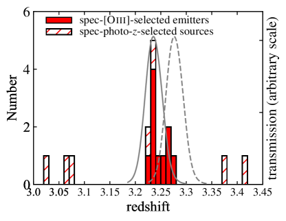
Figure 1: Redshift distribution of the spectroscopically confirmed sources from this observation. The filled histogram shows the [Oiii] emitters and the hatched histogram shows that of our secondary targets, i.e. the photo-$z$-selected sources. The transmission curves of the ${\rm NB}_{K}$ filter are also shown. The wavelength range of the ${\rm NB}_{K}$ filter is converted to the redshift ranges for the [Oiii]$\lambda$5008 emission line (the solid curve) and the [Oiii]$\lambda$4960 emission line (the dashed curve), respectively.

2.5 Estimation of physical quantities

The stellar masses of the spectroscopically confirmed sources are estimated by SED fitting with the public code EAZY (Brammer et al., 2008) and FAST (Kriek et al., 2009). We use the total magnitudes of 14 photometric bands; $u,B,V,r,i^{\prime},z^{\prime\prime},Y,J,H,K_{s}$, 3.6, 4.5, 5.8, and 8.0 $\mu$m from the COSMOS2015 catalog. We subtract the contributions of the emission lines, the [Oiii] doublet and H$\beta$, and [Oii] doublet, from the $Ks$ and $H$-band magnitudes, respectively, before the SED fitting. When running the FAST, we fix their redshifts to those measured from the spectroscopy. We use the population synthesis models of Bruzual & Charlot (2003) with a Chabrier IMF (Chabrier, 2003), and the dust extinction law of Calzetti et al. (2000). We assume exponentially declining SFHs with ${\rm log(\tau/yr)=}$ 8.5–11.0 in steps of 0.1, and metallicities of $Z=0.004,0.008,$ and 0.02 (solar).

SFRs are estimated from UV continuum luminosities in order to compare with a whole sample of [Oiii] candidate emitters (Figure 3). Dust extinction is corrected for using the slope of the rest-frame UV continuum spectrum (e.g. Meurer et al. 1999; Heinis et al. 2013). The UV slope $\beta$ is defined as $f_{\lambda}$$\propto$$\lambda^{\beta}$. We estimate $\beta$ by fitting a linear function to the five broad-bands from the $B$ to $i$-band. The slope $\beta$ is converted to dust extinction $A_{\rm FUV}$ with the following equation from Heinis et al. (2013):

$$A_{\rm FUV}=3.4+1.6\beta.$$ (5)

Then, the intrinsic flux density $f_{\nu,{\rm int}}$ is obtained from

$$f_{\nu,{\rm int}}=f_{\nu,{\rm obs}}\ 10^{0.4A_{\rm FUV}}.$$ (6)

${\rm SFR_{UV}}$ is estimated from the $r$-band ($\lambda_{\rm c}=6288.7\ \mathrm{\AA}$ which corresponds to $\lambda_{\mathrm{0}}=1500\mathrm{\AA}$ at $z=3.2$) magnitude using the equation from Madau et al. (1998):

$${\rm SFR\ (M_{\odot}yr^{-1})} = \frac{4\pi D_{L}^{2}f_{\nu,{\rm int}}}{(1+z)\times 8\times 10^{27}\ ({\rm erg\ s^{-1}cm^{-2}Hz^{-1}})}$$ (7)

$$= \frac{L({1600}{\rm\AA})}{8\times 10^{27}\ ({\rm erg\ s^{-1}Hz^{-1}})},$$

where $D_{L}$ is the luminosity distance. Considering the difference between Chabrier and Salpeter (Salpeter, 1955) IMFs, we divide the SFRs by a factor of 1.7 (Pozzetti et al., 2007) so that we always use Chabrier IMF throughout this paper.

For the two photo-$z$-selected sources, which are not included in the COSMOS2015 catalog, we use the photometric data ($u,B,V,g,r,i,z,J,K$) from the catalog of Ilbert et al. (2009). The estimated stellar mass, dust extinction, and $\mathrm{SFR_{UV}}$ for each galaxy are summarized in Appendix-A.

Comparing the estimated $\rm SFR_{UV}$ with those obtained by FAST, the results of the SED fitting show a systematic offset of $\sim+0.25$ dex with respects to those obtained from the rest-frame UV luminosities. Since we compare SFRs obtained with the same method in Section 2.6, such a systematic offset does not affect our results. As for $A_{\rm FUV}$, there is no systematic offset and differences between the two methods are within 0.4 mag.

In addition to $\mathrm{SFR_{UV}}$, we also estimate SFRs from the H$\beta$ luminosities. The dust extinction for H$\beta$ is corrected for by using the UV slope $\beta$ (Heinis et al., 2013), and the Calzetti extinction law (Calzetti et al., 2000) assuming $E(B-V)_{\rm nebular}=E(B-V)_{\rm stellar}$ (e.g. Erb et al., 2006b; Reddy et al., 2010, 2015). We convert the dust-extinction-corrected H$\beta$ luminosity to the H$\alpha$ luminosity using the intrinsic H$\alpha$/H$\beta$ ratio of 2.86 under the assumption of Case B recombination with a gas temperature $T_{e}=10^{4}$ K and an electron density $n_{e}=10^{2}\ {\rm cm^{-3}}$ (Osterbrock & Ferland, 2006).

Then we convert the estimated H$\alpha$ luminosities to SFRs using the equation from Kennicutt & Evans (2012);

$$\mathrm{log(SFR_{H\alpha}/M_{\odot}yr^{-1})}=\mathrm{log}(L_{\mathrm{H\alpha}}/\mathrm{erg\ s^{-1}})-41.27.$$ (8)

Here we account for the difference between the Chabrier and Kroupa IMF by subtracting 0.013 dex (Pozzetti et al., 2007; Marchesini et al., 2009).

In Figure 2, we compare the two SFRs derived from UV and H$\beta$ luminosities. We find that the two SFRs derived from UV luminosities and from H$\beta$ luminosities have similar values within a factor of two except for a few sources. The mean $\rm SFR_{H\beta}/SFR_{UV}$ for our sample is $1.6\pm 0.2$. We can estimate their SFRs reasonably well from the UV luminosities with dust correction based on the UV slope at $z>3$.

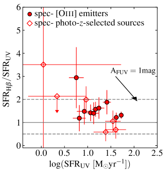
Figure 2: $\mathrm{SFR_{UV}}$ versus $\mathrm{SFR_{H\beta}/SFR_{UV}}$ ratio of our spectroscopically confirmed galaxies. Here we do not consider the extra extinction to the nebular emission, i.e. we assume $E(B-V)_{\rm nebular}=E(B-V)_{\rm stellar}$ (e.g. Erb et al., 2006b; Reddy et al., 2010, 2015). Dust extinction is corrected for by using the UV slope $\beta$ (Eq. 5). The solid line represents the case where the two SFRs are identical, and the dashed lines represent the cases where the difference between the two is a factor of two. The arrow shows how dust correction with $\mathrm{A_{FUV}=1~{}mag}$ moves the points on this diagram. For most of our targets, SFRs derived from the two different indicators are identical with each other within a factor of two.

2.6 Stellar mass–SFR relation

In Figure 3 we show the relation between the stellar masses and $\mathrm{SFR_{UV}}$ of the spectroscopically confirmed galaxies in this studies together with the [Oiii] candidate emitters at $z\sim 3.24$ from HiZELS. This figure shows that our targets are not biased towards a particular region on the stellar mass–$\mathrm{SFR_{UV}}$ diagram with respect to the parent sample of the [Oiii] emitters at $z\sim 3.24$. This indicates that they are normal star-forming galaxies at the epoch.

We also show the [Oiii] candidate emitters at $z\sim 2.23$ after matching the ${\rm NB}_{H}$ emitter catalog in the COSMOS field from HiZELS (Sobral et al., 2013) with the COSMOS2015 catalog. The selection criteria of the ${\rm NB}_{H}$ emitters are the same as those mentioned in Section 2.1 with the ${\rm NB}_{H}$ filter being used instead of the ${\rm NB}_{K}$(Sobral et al., 2013). We select [Oiii] candidate emitters at $z\sim 2.23$ with photometric redshifts of $1.7<z_{\rm photo}<2.8$. We also employ the color–color diagrams ($BzK$, $izK$, and $UVz$) for the emitters with no photometric redshifts as introduced in Khostovan et al. (2015). We obtained 117 [Oiii] candidate emitters at $z\sim 2.23$ in total.

Stellar masses and $\rm SFR_{UV}$ of the [Oiii] candidate emitters at $z\sim 3.24$ and $z\sim$2.23 are estimated following the same procedure as described in Section 2.5. As for [Oiii] emitters at $z\sim 2.23$, we use the $V$-band magnitude to estimate $\rm SFR_{UV}$. The redshift is fixed of each source is fixed to $z=3.24$ or 2.23. We note that we take into account the different luminosity limit of the [Oiii] emission line when comparing the [Oiii] emitters at different redshifts in Figure 3.

We find that the [Oiii] emitters at $z\sim 3.24$ show similar SFRs as those of [Oiii] emitters at $z\sim 2.23$ at a fixed stellar mass. The distribution of the [Oiii] candidate emitters at $z\sim 2.23$ is consistent with the fit to the [Oiii] candidate emitters at $z\sim 3.24$ statistically. While the normalization of the stellar mass–SFR relation is almost consistent, the distribution along the relation seems to be different. The [Oiii] emitters at $z\sim 3.24$ show an offset towards the lower stellar mass range as seen in the top and right panels of Figure 3 (Suzuki et al. 2015; comparison between the [Oiii] emitters at $z\sim 3.2$ and the H$\alpha$ emitters at $z\sim 2.2$).

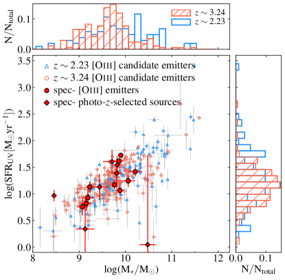
Figure 3: Relation between stellar mass and $\mathrm{SFR_{UV}}$. The spectroscopically confirmed galaxies in this study are identified. [Oiii] candidate emitters at $z\sim 3.24$ (open circles) and $z\sim 2.23$ (open triangles) in the COSMOS field are also shown. Top and right histogram shows the stellar mass and SFR distribution, respectively. Hatched and open histograms correspond the [Oiii] candidate emitters at $z\sim 3.24$ and $z\sim 2.23$, respectively. The spectroscopically confirmed [Oiii] emitters are not biased towards a particular region on the stellar mass–$\mathrm{SFR_{UV}}$ plane with respect to the parent sample at $z\sim 3.24$.

2.7 Stacking analysis

In order to investigate the averaged properties of the [Oiii] emitters at $z\sim 3.2$, we carry out the stacking analysis of the spectra by dividing the ten [Oiii] emitters into two stellar mass bins, i.e. $9.76\leq\mathrm{log(M_{*}/M_{\odot})}\leq 10.21$ and $9.07\leq\mathrm{log(M_{*}/M_{\odot})}\leq 9.23$.

We transform the individual spectra to the rest-frame wavelength based on the derived redshifts, and normalize them by integrated [Oiii]$\lambda$5008 flux. The wavelength dispersion of the spectrum in $K$ and $H$-band is 2.1719 Å/pix and 1.6289 Å/pix, respectively. When converting them to the rest-frame spectra, we fix the wavelength interval to 0.25 Å, and interpolate the spectra linearly. Noise spectra for the individual galaxies are also scaled by integrated [Oiii]$\lambda$5008 flux, and are similarly converted to the rest-frame wavelength. Then, the stacking of the individual spectra is carried out with the following equation:

$$f_{\mathrm{stack}}=\sum_{i}^{N}\frac{f_{i}(\lambda)}{\sigma_{i}(\lambda)^{2}}/\sum_{i}^{N}\frac{1}{\sigma_{i}(\lambda)^{2}},$$ (9)

where $f_{i}(\lambda)$ is a flux density of the individual spectra and $\sigma_{i}(\lambda)$ is a sky noise as a function of the wavelength (Shimakawa et al., 2015b). The noise spectrum for the stacked spectrum is calculated by an error propagation from the individual noise spectra. The stacked spectra in the two stellar mass bins are shown in Figure 4.

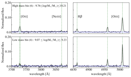
Figure 4: Stacked spectra of the [Oiii] emitters obtained by dividing the samples into two stellar mass bins of $9.76\leq\mathrm{log(M_{*}/M_{\odot})}\leq 10.21$ and $9.07\leq\mathrm{log(M_{*}/M_{\odot})}\leq 9.23$. The stacked spectra are shown by the gray curves. The blue curves represent the 1$\sigma$ sky noise. We show the [Oii] doublet and the [Neiii] in the left panel, and the H$\beta$ and the [Oiii] doublet in the right panel, respectively.

3 ISM conditions of [OIii] emitters among other samples at $z>3$

3.1 Line ratios and its stellar mass-dependence at $z>3$

The left panel of Figure 5 shows the relation between two line ratios, namely, the $R_{\mathrm{23}}$-index (([Oiii]$\lambda\lambda$5008,4960 + [Oii]) / H$\beta$) and [Oiii]$\lambda\lambda$5008,4960/[Oii] ratio. While the $R_{\rm 23}$–index and [Oiii]/[Oii] ratio depend on both the gas metallicity and ionization parameter, the $R_{\rm 23}$ is more sensitive to the gas metallicity and [Oiii]/[Oii] is more sensitive to the ionization parameter (e.g. Kewley & Dopita, 2002; Nakajima & Ouchi, 2014).

We show our sample on the $R_{\rm 23}$–[Oiii]/[Oii] diagram together with star-forming galaxies at the same epoch from the literature, namely, UV-selected galaxies from Onodera et al. (2016) and LAEs from Nakajima et al. (2016). The model predictions are also shown on the diagram. The theoretical line ratios in the Hii regions are estimated using the photoionization code MAPPINGS V (MAPPINGS; Sutherland & Dopita 1993). In the MAPPIGNS, we assume a Hii region with a constant pressure of $P/k=10^{6.5}{\rm cm^{-3}\ K}$, where $k$ is the Boltzmann constant. The temperature of the Hii region is set to be $\sim 10^{4}$ K, and then the density becomes $\sim$ 300 ${\rm cm^{-3}}$, which corresponds to the typical electron density of star-forming galaxies at high redshifts (e.g. Steidel et al., 2014; Shimakawa et al., 2015b; Sanders et al., 2016b; Onodera et al., 2016; Strom et al., 2017). We change the metallicity and ionization parameter independently as follows: $Z=0.05,\ 0.2,\ 0.4,\ 1.0,\ 2.0\ Z_{\odot}$, and log($q\ [{\rm cms^{-1}}]$) = 8.35, 8.00, 7.75, 7.50, 7.25, and 7.00.

In this paper, we use the ionization parameter defined as:

$$q=\frac{Q_{\rm H^{0}}}{4\pi R_{\rm s}^{2}n_{\rm H}},$$ (10)

where $Q_{\rm H^{0}}$ is the flux of the ionizing photons produced by the existing stars above the Lyman limit, $R_{\rm s}$ is the Strömgren radius, and $n_{\rm H}$ is the local density of hydrogen atoms (Kewley & Dopita (2002); and see also Sanders et al. (2016b) for detailed discussions about the definitions of the ionization parameter).

In the right panel of Figure 5, we show the relation between the stellar mass and the [Oiii]$\lambda\lambda$5008,4960/[Oii] ratio of the same samples shown in the left panel in order to clarify the differences in the stellar mass distributions among the samples.

In Figure 5, we also show local star-forming galaxies from SDSS Data Release 8 (DR8), whose physical quantities are provided by the MPA-JHU group (Abazajian et al., 2009; Aihara et al., 2011). We clearly see that star-forming galaxies at $z>3$ show very different line ratios from those of local star-forming galaxies, in the sense that those of $z>3$ galaxies tend to have higher [Oiii]/[Oii] ratios at a fixed $R_{\mathrm{23}}$-index and stellar mass. This confirms the results already reported in the literature using the UV-selected galaxies that the ionization states of star-forming galaxies at $z>3$ are higher than those of star-forming galaxies at $z=0$ (e.g. Holden et al., 2016; Onodera et al., 2016; Nakajima et al., 2016).

When we compare our sample to the sample of Onodera et al. (2016) in Figure 5, there is no clear difference between the two samples. The [Oiii] emitters are not systematically biased towards higher $R_{\mathrm{23}}$-index or higher [Oiii]/[Oii] ratios with respect to the UV-continuum-selected star-forming galaxies at the same epoch. When comparing the LAEs at $z\sim 3$ from Nakajima et al. (2016), at a lower stellar mass regime of $\mathrm{log(M_{*}/M_{\odot})}\sim 9.0$, the [Oiii] emitters are likely to be consistent with being the same population as LAEs. Our results suggest that the selection based on the [Oiii] emission line strength does not cause any significant bias in terms of the ISM conditions, and moreover, that we can pick up star-forming galaxies in a wide range of ISM conditions from ones with extreme conditions such as LAEs to ones with moderate conditions at $z>3$.

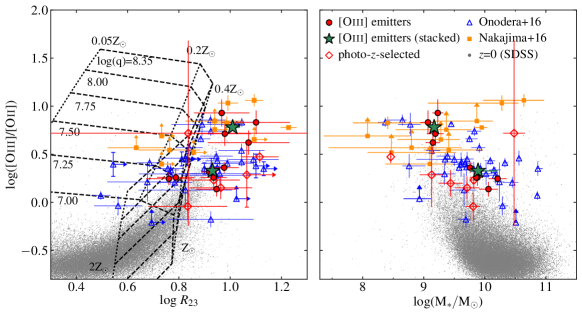
Figure 5: Relation between the $R_{\mathrm{23}}$-index and [Oiii]$\lambda\lambda$5008,4960/[Oii] ratio (left) and between the stellar mass and the [Oiii]$\lambda\lambda$5008,4960/[Oii] ratio (right) of our sample at $z\sim 3.2$, [Oiii] emitters and photo-$z$-selected sources. We also plot UV-selected star-forming galaxies at $z=3-3.7$ from Onodera et al. (2016), LAEs at $z\sim 3$ from Nakajima et al. (2016), and local star-forming galaxies from SDSS (Abazajian et al., 2009; Aihara et al., 2011). In the left panel, the dashed and dotted lines represent the model prediction of the $R_{23}$-index and the [Oiii]/[Oii] ratio calculated using the photoionization code MAPPINGS V. Star-forming galaxies at $z>3$ have different ISM conditions from those of local star-forming galaxies. Comparing among samples at $z>3$, massive [Oiii] emitters ($\mathrm{log(M_{*}/M_{\odot})}\sim$ 9.8–10.2) seem to show similar line ratios as UV-selected galaxies, while less massive [Oiii] emitters ($\mathrm{log(M_{*}/M_{\odot})}\sim 9.0$) are similar to LAEs. When H$\beta$ is detected with S/N $<3.0$, we replace it with the 3$\sigma$ flux limit. The source not detected with H$\beta$ is not shown in the left panel.

3.2 Metallicity estimation with the empirical calibration method

We use the fully empirical relations calibrated using local star-forming galaxies from SDSS by Curti et al. (2017). They introduced the empirical relations between the gaseous metallicities and six line ratios, and in this study, we use four line ratios with [Oiii], H$\beta$, and [Oii] lines. Hereafter, we estimate gas metallicities only for the sources with all of these emission lines being detected with S/N $\geq 3$. Also, we remove the source with a large uncertainty of $\rm A_{FUV}$. Note that all of the removed sources are the photo-$z$-selected sources.

We fit the four line ratios simultaneously, and determine the best-fit metallicity that can minimize the $\chi^{2}$ value. Here the $\chi^{2}$ is defined as follows:

$$\chi^{2}=\sum_{i=1}^{N}\frac{(\mathrm{log}\ R_{i,\mathrm{obs}}-\mathrm{log}\ R_{i,\mathrm{fit}})^{2}}{\sigma^{2}_{i,\mathrm{obs}}+\sigma^{2}_{i,\mathrm{int}}},$$ (11)

where log $R_{i,\mathrm{obs}}$ and log $R_{i,\mathrm{fit}}$ are the $i$-th line ratio obtained from the observed spectra and one obtained from the relation of Curti et al. (2017) at a given metallicity (Onodera et al., 2016). $\sigma_{i,\mathrm{obs}}$ is the error of each line ratio from the observed spectra, and $\sigma_{i,\mathrm{int}}$ is the intrinsic scatter of a line ratio at a given metallicity, respectively. We apply the root-mean-square estimated for each relation (Table 2 in Curti et al. (2017)) as the intrinsic scatter. In Figure 6, we show the relations between the metallicity, which is determined with two different calibration methods, and line ratios. Note that the four line ratios shown in Figure 6 are not independent, and the 1$\sigma$ errors in the metallicities are determined from values of 12+log(O/H) with $\Delta\chi^{2}=3$ compared to the best fit solution.

We note that locally calibrated relations between line ratios and gas metallicity might not be applicable to star-forming galaxies at high redshifts because their typical ISM conditions seem to change from $z=0$ (Kewley et al. 2013; Nakajima & Ouchi 2014; Steidel et al. 2014; Strom et al. 2017; Kashino et al. 2017 and Figure 5), while some previous studies have suggested that physical conditions of Hii regions do not evolve with redshifts at a fixed metallicity (e.g. Jones et al., 2015; Sanders et al., 2016a). Nevertheless, since it is shown that the gas metallicities estimated with different line ratios show systematic offsets from one another (Kewley & Ellison, 2008), we here use the locally calibrated empirical relations to estimate gas metallicities for a fair comparison with Onodera et al. (2016) in the next section.

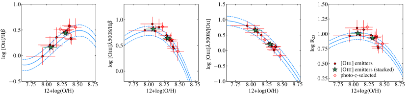
Figure 6: Relations between four line ratios and metallicities calibrated with the Curti et al. (2017) method. The solid curve in each panel represents the relation derived in Curti et al. (2017). The dashed curves represent the root-mean-square of their fit. The four line ratios of individual galaxies are well fitted by their empirical relations within 1$\sigma$ errors.

3.3 Mass–Metallicity relation at $z>3$

In Figure 7, we show the relation between stellar mass and gas metallicity for our sample. As already shown in a number of previous studies, stellar mass and metallicity of our galaxies at $z\sim 3.2$ show a correlation such that more massive galaxies have higher metallicities (e.g. Tremonti et al. 2004; Erb et al. 2006a; Maiolino et al. 2008; Stott et al. 2013; Zahid et al. 2013, 2014; Steidel et al. 2014; Troncoso et al. 2014; Sanders et al. 2015). UV-selected galaxies at the same epoch from the Onodera et al. (2016) are also shown. We find no clear difference of gas metallicities between the [Oiii] emitters and the UV-selected galaxies at a fixed stellar mass.

As also suggested in Figure 5, [Oiii] emitters are not biased towards a particular population with respect to their ISM conditions and metal contents as compared to the UV-continuum-selected galaxies at least in the stellar mass range covered by our observation, i.e. $\mathrm{log(M_{*}/M_{\odot})}\sim$ 9.0–10.2. It is expected that the effect of dust extinction is not significant in our stellar mass range, and therefore, there is no difference between the [Oiii]-selected and the UV-selected galaxies. If the [Oiii]-selected galaxies can trace more massive and dustier star-forming galaxies, the difference might appear in more massive stellar mass range, and a larger sample of the [Oiii] emitters and their follow-up observations are required.

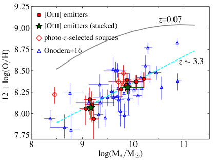
Figure 7: Relation between stellar mass and gas metallicity for our sample at $z\sim 3.2$ and the UV-selected galaxies at $z\sim$ 3–3.7 from Onodera et al. (2016). The solid curve represents the mass–metallicity relation at $z=$ 0.07 (Maiolino et al., 2008). The dashed curve represents the best-fitted mass–metallicity relation at $z\sim 3.3$ from Onodera et al. (2016). Our targets are well below the mass–metallicity relation of the local star-forming galaxies. Comparing with the UV-selected galaxies at the same epoch, there is no clear difference of gas metallicities at a fixed stellar mass between the two samples. Our [Oiii] emitters well follow the best-fitted relation by Onodera et al. (2016).

4 Comparison with star-forming galaxies at $z\sim 2$

4.1 Metallicity calibration based on photoionization modelling

We apply the calibration method, which is introduced by Kobulnicky & Kewley (2004, KK04), as well as the empirical calibration method by Curti et al. (2017) as described in Section 3.2 in order to compare our sample with previous studies at $z\sim 2$ in the following sections.

KK04 used strong emission lines and determined relations between line ratios, gas metallicities and ionization parameters based on the photoionization model, MAPPINGS. In this method, the gas metallicity and ionization parameter are determined simultaneously using the two line ratios of the $R_{\mathrm{23}}$-index and [Oiii]/[Oii].

We estimate the gas metallicity and ionization parameter by following KK04. The relation between ionization parameter $\mathrm{log(q)}$ and [Oiii]$\lambda\lambda$5008,4960/[Oii] ratio is given by

$$\mathrm{log} (q)=\{32.81-1.153y^{2}$$

$$+ [12+\mathrm{log(O/H)}](-3.396-0.025y+0.1444y^{2})$$

$$\times \{4.603-0.3119y-0.163y^{2}$$

$$+ [12+\mathrm{log(O/H)}](-0.48+0.0271y+0.02037y^{2})\}^{-1},$$

where $y=\mathrm{log([\textsc{Oiii}]\lambda\lambda 5008,4960/[\textsc{Oii}])}$. The relation between gas metallicity 12+log(O/H) and the $R_{\mathrm{23}}$-index is separated into the two equations according to gas metallicity. At the lower metallicity branch of ${\rm 12+log(O/H)}<8.4$,

$$12+\mathrm{log(O/H)_{lower}} = 9.40+4.65x-3.17x^{2}$$

$$- \mathrm{log}(q)(0.272+0.547x-0.513x^{2}),$$

and at the upper metallicity branch of ${\rm 12+log(O/H)}\geq 8.4$,

$$12 + \mathrm{log(O/H)_{upper}}=9.72-0.777x-0.951x^{2}$$ (14)

$$- 0.072x^{3}-0.811x^{4}-\mathrm{log}(q)(0.0737-0.0713x$$

$$- 0.141x^{2}+0.0373x^{3}-0.058x^{4}),$$

where $x=\mathrm{log}R_{\rm 23}$. Consistent metallicity and ionization parameter are determined in an iterative manner using Eq.(4.1) and Eq.(4.1) or Eq.(14) according to the value of 12+log(O/H) (KK04).

We compare gas metallicities obtained by the KK04 method with those obtained in Section 3.2. When we see the upper metallicity branch, the gas metallicities based on the photoionization models are systematically higher ($\sim 0.25\ {\rm dex}$) than those from the empirical relations. As for the solutions at the lower metallicity branch, there is no systematic offset with respect to the results from the empirical relations but they seem to show a negative trend with respect to the stellar mass (Appendix B).

In order to determine the metallicity branch at a given $R_{\rm 23}$-index, an additional line ratio, such as [Nii]/[Oii], is required (KK04). Since we cannot observe [Nii]$\lambda$6585 lines for $z>3$ galaxies from the ground, it is difficult to determine the metallicity branch for each object in our sample. In the following sections, we only show the gas metallicities at the upper branch for clarity.

We note that Steidel et al. (2014) suggested the possibility that metallicity calibration methods using the $R_{\mathrm{23}}$-index do not work well in the metallicity range of $\mathrm{12+log(O/H)}=$ 8.0–8.7. However, here we use the KK04 method due to the limited available emission lines of our sample and also for a fair comparison with previous studies at $z\sim 2$. Kewley & Ellison (2008) showed that the gas metallicities with the calibration methods using different line ratios show systematic offsets from one another. Therefore, we attempt to compare gas metallicities estimated with the same calibration method.

4.2 Comparison of the ionization parameter and gas metallicity

In Figure 8 (a), we show gas metallicities and ionization parameters of our sample estimated in Section 4.1. Here we show the two solutions at the upper and lower metallicity branch while some sources have the same solution at the two branches indicating that they lie at the cross-over metallicity. We also show the results of LBGs and LAEs at $z\sim$ 2–3 from Nakajima & Ouchi (2014), who estimated gas metallicities and ionization parameters with the KK04 method. Comparing our sample with LBGs and LAEs of Nakajima & Ouchi (2014) on this diagram, our sample at $z\sim 3.2$ shows similar gas metallicities and ionization parameters as those of the LBGs at $z\sim$ 2–3.

In Figure 5, we find that star-forming galaxies at $z>3$ clearly show different line ratios from those of the local star-forming galaxies, indicating that they are likely to have higher ionization parameters at a fixed metallicity or stellar mass. Figure 8 (a) indicates that the redshift evolution of ISM conditions is unlikely to be strong between $z\sim 3.2$ and $z\sim 2$. The sample of LBGs of Nakajima & Ouchi (2014) covers a wider stellar mass range than that of our sample, $\mathrm{log(M_{*}/M_{\odot})=8.0-10.8}$. We also note that their LBG sample includes galaxies at $z\sim 3$ from AMAZE (Maiolino et al., 2008), and this might contribute to similar ionization parameters and gas metallicities between the two samples.

4.3 Comparison of mass–metallicity relation

In Figure 8 (b), we show the relation between stellar mass and gas metallicity again, but gas metallicities are estimated with the KK04 method for a fair comparison with previous studies about star-forming galaxies at $z\sim 2$ (Zahid et al., 2013; Cullen et al., 2014; Steidel et al., 2014; Sanders et al., 2015).

We introduce some previous studies at $z\sim 2$. Cullen et al. (2014) investigated ISM conditions of star-forming galaxies at $z\sim 2.2$ selected from the 3D-HST grism survey data. Their sample is basically selected by their strong [Oiii] emission lines. They stacked their samples into six stellar mass bins and measured the fluxes of the [Oii], H$\beta$, and [Oiii] lines. We here directly estimate gas metallicities of their sample with the KK04 method. We show the solutions at the upper metallicity branch in Figure 8 (b).

We also show the results from Steidel et al. (2014) and Sanders et al. (2015), who calibrated gas metallicities using the [Nii]/H$\alpha$ lines ratios (N2) by Pettini & Pagel (2004, PP04). We converted their gas metallicities using the formula given by Kewley & Ellison (2008) so that gas metallicities correspond to those estimated using the KK04 method. We show one more previous study, Zahid et al. (2013). They obtained the mass–metallicity relation at $z\sim 2.2$ with the KK04 method by converting the mass–metallicity relation obtained by Erb et al. (2006a) with the N2 (PP04) method with the formula by Kewley & Ellison (2008).

The thick dash-dotted line in Figure 8 (b) shows the best-fitted mass–metallicity relation derived using the solutions at the upper metallicity branch of our sample at $z\sim 3.2$. We compare this best-fitted relation at $z\sim 3.2$ with that estimated for Cullen et al. (2014) sample. The slopes and intercepts of the best-fitted lines for the two samples are consistent with each other within errors, indicating that the gas metallicities of our sample at $z\sim 3.2$ are similar those of star-forming galaxies at $z\sim 2.2$ at a fixed stellar mass. This is also the case when comparing the solutions at the lower metallicity branch (Appendix B).

On the other hand, comparing with other previous studies, which estimated gas metallicity with N2 (PP04) method originally, they tend to have higher metallicities with respect to our sample and the sample of Cullen et al. (2014). It is suspected that there is still a systematic difference due to using different calibration methods even after the correction. The correction factors for local star-forming galaxies introduced in Kewley & Ellison (2008) might not be applicable for star-forming galaxies at $z>2$ due to their different physical conditions. Therefore, comparing our targets with the samples whose metallicities are originally calibrated by the N2 (PP04) method might not be fair. We conclude that our sample at $z\sim 3.2$ has similar ISM conditions and mass–metallicity relation as star-forming galaxies at $z\sim 2$ under the same calibration method.

4.4 ISM conditions and star-forming activity between $z\sim 3.2$ and $z\sim 2$

In Figure 3, we show that the normalization of star-forming main sequence seems to be similar at $z\sim 3.2$ and $z\sim 2$. Also, as shown in Figure 8, it is suggested that the ISM conditions and the mass–metallicity relation do not seem to evolve between the two epochs. These results suggest that the properties of star-forming galaxies at $z\sim$ 2.0–3.2 (the difference of cosmic age of $\sim 1.3$ Gyr) are primarily determined by their stellar masses rather than cosmic epoch since galaxies are very young and their ages are getting closer to the age of the Universe ($\sim$ a few Gyr).

As discussed in Suzuki et al. (2015) and as suggested distributions between the [Oiii] emitters at $z\sim 3.2$ and $z\sim 2.2$ along the main sequence (Figure 3), the individual galaxies should experience significant growth in stellar masses. These results probably reflect that galaxies are in the vigorous formation phase at this epoch, and such a significant growth must be supported by ample gas accretion from the outside throughout these early epochs (e.g. Kereš et al., 2005, 2009; Dekel et al., 2009; Bouché et al., 2010).

Onodera et al. (2016) also showed that the gas metallicity difference between their sample at $z>3$ and Cullen et al. (2014) sample at $z\sim 2.2$ is relatively small at a fixed stellar mass. They found that a simple gas regulator model with mildly evolving star formation efficiency (Lilly et al., 2013) could well predict the observational trend of the redshift evolution of the mass–metallicity relation.

By obtaining the gas mass fractions for our sample and combining them with gas metallicities and stellar masses, it will become possible to give constraints on the inflow and outflow rates by combining with gas metallicities and stellar masses (e.g. Troncoso et al., 2014; Yabe et al., 2015; Seko et al., 2016). Dust continuum or CO line observations with ALMA will enable us to directly measure the molecular gas mass of individual galaxies at $z>3$.

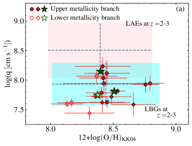
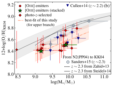
Figure 8: (a) Gas metallicity and ionization parameter of our sample at $z\sim 3.2$ estimated using the KK04 method (circles: [Oiii] emitters and diamonds: photo-$z$-selected sources). The two solutions are shown with the filled (upper metallicity branch) and open (lower metallicity branch) symbols. The stacking results of the [Oiii] emitters are shown with the star symbols. The blue and red shaded region shows the results of the LBGs and LAEs at $z\sim$ 2–3, respectively, from Nakajima & Ouchi (2014). The same method is applied here. Our targets at $z>3$ seem to cover a similar range of gas metallicity and ionization parameter as that of the LBGs at $z\sim$ 2–3.
(b) Relation between stellar mass and gas metallicity for our sample at $z\sim 3.2$. We estimate gas metallicities with the KK04 method here, and the solutions at the upper metallicity branch are shown. The dash-dotted line shows the best-fitted line derived for our sample. We compare our sample at $z\sim 3.2$ with previous studies about star-forming galaxies at $z\sim 2$. Except for the sample of Cullen et al. (2014), gas metallicities are originally calibrated with N2 (PP04) method and then are converted using a formula by Kewley & Ellison (2008) (Zahid et al., 2013; Steidel et al., 2014; Sanders et al., 2015). The red and gray shaded region corresponds to $\pm 1\sigma$ errors of the best-fitted relation of our sample using results at upper metallicity branch and Steidel et al. (2014), respectively. The mass–metallicity relation of our sample is consistent with that of Cullen et al. (2014) within 1$\sigma$ error.

5 Summary

In this paper, we present the results from NIR spectroscopic follow-up of star-forming galaxies at $z\sim 3.2$. Our primary targets are the NB-selected [Oiii] emission line galaxies obtained by HiZELS in the COSMOS field (Sobral et al., 2013; Khostovan et al., 2015). We obtain $H$ and $K$ band spectra of all ten [Oiii] emitters and seven photo-$z$-selected galaxies (our secondary targets). Our results demonstrate the high efficiency of follow-up observations of NB-selected galaxies with all candidates being confirmed as [Oiii] emitters. By exploiting our deep NIR spectra, we find that:

1. In comparison with local galaxies, our sample shows different ISM conditions, such as higher $R_{\mathrm{23}}$-index and higher [Oiii]/[Oii] ratio, and lower gas metallicity at a fixed stellar mass, consistent with many previous studies (e.g. Troncoso et al., 2014; Nakajima & Ouchi, 2014; Steidel et al., 2014; Onodera et al., 2016).

2. We compare our spectroscopically confirmed galaxies at $z\sim 3.0-3.5$ with other galaxy populations at similar redshifts (Onodera et al., 2016; Nakajima et al., 2016) on the $R_{\mathrm{23}}$-index – [Oiii]/[Oii] ratio diagram and the stellar mass–[Oiii]/[Oii] ratio diagram. The [Oiii] emitters show broadly similar line ratios as UV-selected galaxies. Moreover, the line ratios of less massive [Oiii] emitters ($\mathrm{log(M_{*}/M_{\odot})}\sim 9.0$) are consistent with those of LAEs. The [Oiii]-selection seems to cause no significant bias in terms of the ISM conditions, and the [Oiii]-selected galaxies can cover a wide range of stellar masses and ISM conditions of star-forming galaxies at $z>3$. The mass–metallicity relation of our sample is consistent with that of Onodera et al. (2016).

3. We also compare our sample at $z\sim 3.2$ with star-forming galaxies at $z\sim 2$ from literature (Zahid et al., 2013; Cullen et al., 2014; Nakajima & Ouchi, 2014; Steidel et al., 2014; Sanders et al., 2015). Our sample shows similar ionization parameters, gas metallicities, and mass–metallicity relation as those obtained by Nakajima et al. (2016) and Cullen et al. (2014) using the same calibration method. This suggests that the ISM conditions of star-forming galaxies do not strongly evolve at a fixed stellar mass between $z\sim 3.2$ and $z\sim 2.2$. Considering that the [Oiii] emitters at $z\sim 3.2$ have similar SFRs as those at $z\sim 2.2$ at a fixed stellar mass, our results support the idea that the evolutionary stages of star-forming galaxies, such as SFRs and ISM conditions, at $z\gtrsim 2$ are primarily determined by their stellar masses rather than redshift.

Since our current spectroscopic sample is very small, it is necessary to carry out more observations on a larger sample in order to statistically reveal the evolution of ISM conditions and star-forming activities from $z>3$ to $z\sim 2$. The low contamination of the NB-selected emitters will lead to high efficient follow-up observations making it ideal for such studies.

Appendix A $H$ and $K$-band spectra

In Figure 9 and 10, we show the $H$ and $K$-band spectra of the individual sources, namely the [Oiii] emitters ($z_{\mathrm{spec}}=$ 3.23–3.27) and the photo-$z$-selected galaxies ($z_{\mathrm{spec}}=$ 3.03–3.42). The emission line fitting results with a Gaussian component is shown in the red curves, and the results of the emission line fit are summarized in Table 1. In Table 2, we summarize the estimated physical quantities, such as stellar masses, dust extinctions, $\mathrm{SFR_{UV}}$, and correction factors for stellar absorption for H$\beta$.

Figure 9: The $H$ and $K$-band spectra and the emission line fitting results of the ten [Oiii] emitters. The reduced spectra are shown with the gray curves. The blue shaded regions represent the 1$\sigma$ sky noise. The emission line fitting result with a Gaussian component is shown with the red curves for each source. Three panels show the emission lines, [Oii]$\lambda$3727, [Oii]$\lambda$3730 (left panel), [Neiii]$\lambda$3870 (middle panel), and H$\beta$, [Oiii]$\lambda$4960, and [Oiii]$\lambda$5008 (right panel), respectively. We can see that the [Oiii] doublet, H$\beta$, and [Oii] doublet lines are clearly detected with high signal-to-noise ratios for most of the [Oiii] emitters.

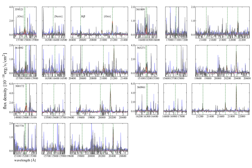
Figure 10: The $H$ and $K$-band spectra and the emission line fitting results of the seven photo-$z$-selected galaxies at $z_{\mathrm{spec}}=3.00-3.45$. he reduced spectra are shown with the gray curves. The blue shaded regions represent the 1$\sigma$ sky noise. The emission line fitting result with a Gaussian component is shown with the red curves for each source. Three panels show the emission lines, [Oii]$\lambda$3727, [Oii]$\lambda$3730 (left panel), [Neiii]$\lambda$3870 (middle panel), and H$\beta$, [Oiii]$\lambda$4960, and [Oiii]$\lambda$5008 (right panel), respectively. Comparing the [Oiii] emitters (Figure 9), the [Oiii] fluxes of these galaxies are weaker.

Table 1: Summary of the emission line properties of the confirmed [Oiii] emitters and photo-$z$-selected sources with Keck/MOSFIRE.

ID	$\mathrm{ID_{15}}$	$\mathrm{ID_{S13}}$	R.A.	Dec.	$z_{\rm spec}$	FWHM	$F_{\mathrm{[OIII]\lambda 5008}}$	$F_{\rm H\beta}$	$F_{\rm[OII]}$	$F_{\rm[NeIII]}$
(1)	(2)	(3)	(J2000)	(J2000)		[$\rm km\ s^{-1}$]	(4)	(5)	(6)	(7)
O3E-1	269781	7612	149.9485	1.6946	3.240	227 $\pm$ 6	9.38 $\pm$ 0.17	1.85 $\pm$ 0.16	4.0 $\pm$ 0.4	1.06 $\pm$ 0.17
O3E-2	269719	7612	149.9777	1.6951	3.227	184 $\pm$ 9	4.63 $\pm$ 0.19	0.61 $\pm$ 0.20	1.08 $\pm$ 0.25	$<$ 0.87
O3E-3	269241	7614	149.9751	1.6938	3.230	244 $\pm$ 11	7.19 $\pm$ 0.27	2.45 $\pm$ 0.45	3.5 $\pm$ 0.4	0.75 $\pm$ 0.19
O3E-4	264007	7625	149.9418	1.6861	3.274	163 $\pm$ 5	4.43 $\pm$ 0.11	0.70 $\pm$ 0.08	0.76 $\pm$ 0.16	$<$ 0.38
O3E-5	260873	7632	149.9557	1.6804	3.241	285 $\pm$ 10	5.78 $\pm$ 0.22	1.42 $\pm$ 0.14	3.6 $\pm$ 0.4	0.91 $\pm$ 0.21
O3E-7	293950	7569	149.9887	1.7333	3.268	309 $\pm$ 5	15.51 $\pm$ 0.21	3.51 $\pm$ 0.17	6.4 $\pm$ 0.4	1.41 $\pm$ 0.17
O3E-8	293774	7569	149.9680	1.7332	3.256	232 $\pm$ 13	3.42 $\pm$ 0.19	1.06 $\pm$ 0.11	1.75 $\pm$ 0.27	$<$ 0.32
O3E-9	289770	7577	150.0213	1.7271	3.230	222 $\pm$ 5	10.11 $\pm$ 0.20	1.19 $\pm$ 0.28	1.40 $\pm$ 0.26	0.86 $\pm$ 0.11
O3E-10	278714	7597	149.9417	1.7095	3.264	136 $\pm$ 4	7.28 $\pm$ 0.18	1.10 $\pm$ 0.24	0.77 $\pm$ 0.23	$<$ 0.94
O3E-11	274195	7604	149.9889	1.7018	3.232	262 $\pm$ 5	11.37 $\pm$ 0.18	2.55 $\pm$ 0.26	5.35 $\pm$ 0.26	1.22 $\pm$ 0.13
359521	297273	—	150.0043	1.7389	3.228	232 $\pm$ 12	3.39 $\pm$ 0.16	—	1.92 $\pm$ 0.26	$<$ 0.65
361009	290562	—	150.0045	1.7279	3.415	201 $\pm$ 25	1.49 $\pm$ 0.16	0.54 $\pm$ 0.09	1.36 $\pm$ 0.12	$<$ 0.23
361492	285414	—	149.9428	1.7203	3.234	169 $\pm$ 15	2.29 $\pm$ 0.16	$<$ 0.36	1.15 $\pm$ 0.24	—
363271	281091	—	149.9977	1.7128	3.069	203 $\pm$ 7	4.60 $\pm$ 0.13	1.06 $\pm$ 0.11	2.45 $\pm$ 0.20	$<$ 0.46
368172	259897	—	149.9322	1.6792	3.027	251 $\pm$ 9	8.10 $\pm$ 0.26	1.89 $\pm$ 0.23	3.86 $\pm$ 0.26	0.71 $\pm$ 0.11
360961	—	—	150.0077	1.7288	3.373	146 $\pm$ 4	6.16 $\pm$ 0.14	0.83 $\pm$ 0.08	1.73 $\pm$ 0.15	0.41 $\pm$ 0.08
363778	—	—	149.9730	1.7100	3.078	134 $\pm$ 11	1.56 $\pm$ 0.13	0.30 $\pm$ 0.06	0.29 $\pm$ 0.08	—

(1) For the [Oiii] emitters, IDs are unique in this paper only. For the photo-$z$-selected sources, IDs are extracted from the catalog of Ilbert et al. (2009).
(2) IDs in the COSMOS2015 catalog (Laigle et al., 2016).
(3) IDs in the catalog of ${\rm NB}_{K}$ emitters from HiZELS (Sobral et al., 2013). We only show numbers here while the IDs given in the catalog are “HiZELS-COSMOS-NBK-DTC-S12B-**”.
(4)(5)(6)(7) Fluxes are shown in the unit of $10^{-17}[\rm erg\ s^{-1}cm^{-2}]$, and not corrected for the dust extinction.
(5) The stellar absorption is not corrected for.
(6) [Oii]$\lambda$3726 $+$ [Oii]$\lambda$3729 fluxes
(7) The fluxes with S/N $<$ 3.0 are replaced with the 3$\sigma$ limit values, if a line flux is not listed then it was affected by OH skylines.

Table 2: Summary of the estimated physical quantities of our targets.

ID	$\rm\log(M_{*})$	$\rm A_{FUV}$	$\rm\log(SFR_{UV})$	$f_{\rm corr,H\beta}$
	[$\rm M_{\odot}$]	[mag]	[$\rm M_{\odot}yr^{-1}$]	(1)
O3E-1	9.76 $\pm$ 0.05	0.02 $\pm$ 0.19	1.17 $\pm$ 0.08	1.02
O3E-2	9.15 $\pm$ 0.12	0.0 $\pm$ 0.33	0.82 $\pm$ 0.14	1.07
O3E-3	10.21 $\pm$ 0.15	1.06 $\pm$ 0.20	1.41 $\pm$ 0.09	1.05
O3E-4	9.19 $\pm$ 0.14	0.74 $\pm$ 0.38	0.93 $\pm$ 0.16	1.05
O3E-5	10.06 $\pm$ 0.15	1.06 $\pm$ 0.27	1.24 $\pm$ 0.12	1.05
O3E-7	9.90 $\pm$ 0.06	1.00 $\pm$ 0.10	1.72 $\pm$ 0.04	1.04
O3E-8	9.88 $\pm$ 0.09	0.35 $\pm$ 0.23	1.06 $\pm$ 0.10	1.08
O3E-9	9.07 $\pm$ 0.13	0.30 $\pm$ 0.38	0.76 $\pm$ 0.16	1.03
O3E-10	9.23 $\pm$ 0.09	0.64 $\pm$ 0.25	1.13 $\pm$ 0.10	1.06
O3E-11	9.86 $\pm$ 0.10	1.02 $\pm$ 0.13	1.62 $\pm$ 0.06	1.06
359521	9.44 $\pm$ 0.20	0.67 $\pm$ 0.60	1.13 $\pm$ 0.24	1.14
361009	9.81 $\pm$ 0.12	1.27 $\pm$ 0.65	1.39 $\pm$ 0.26	1.11
361492	9.13 $\pm$ 0.20	0.06 $\pm$ 1.54	0.34 $\pm$ 0.62	1.06
363271	9.71 $\pm$ 0.19	1.99 $\pm$ 0.55	1.61 $\pm$ 0.22	1.05
368172	9.82 $\pm$ 0.06	1.42 $\pm$ 0.41	1.54 $\pm$ 0.17	1.04
360961	8.46 $\pm$ 0.01	1.18 $\pm$ 0.27	0.97 $\pm$ 0.11	1.00
363778	10.48 $\pm$ 0.18	0.0 $\pm$ 4.18	0.04 $\pm$ 1.68	1.21

(1) Correction factor for stellar absorption for H$\beta$. The absorption corrected H$\beta$ fluxes are estimated by multiplying the observed H$\beta$ fluxes by $f_{\rm corr,H\beta}$.

Appendix B Gas metallicities at the two branches of the KK04 method

In Figure 11, we show the two solutions obtained by the KK04 method for our sample and Cullen et al. (2014) sample. Although it is difficult to choose the appropriate branch for our sample with the current data, we note that there is no large difference of gas metallicities at a fixed stellar mass between our sample at $z\sim 3.2$ and Cullen et al. (2014) sample at $z\sim 2.2$ when we compare the solutions at the same branch. This is consistent with what we see in Figure 8 (a).

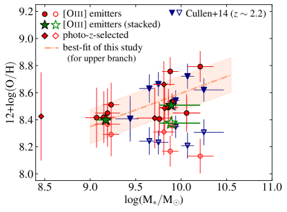
Figure 11: Relation between stellar mass and gas metallicity for our sample at $z\sim 3.2$ and Cullen et al. (2014) sample at $z\sim 2.2$. We show the two solutions obtained by the KK04 method (open symbols: lower metallicity branch, filled symbols: upper metallicity branch). The dash-dotted line is the best-fitted line derived for the solutions at the upper branch, and the shaded region corresponds to $\pm 1\sigma$ errors.

References

- Abazajian et al. (2009) Abazajian, K. N., Adelman-McCarthy, J. K., Agüeros, M. A., et al. 2009, ApJS, 182, 543
- Aihara et al. (2011) Aihara, H., Allende Prieto, C., An, D., et al. 2011, ApJS, 193, 29
- Baldwin et al. (1981) Baldwin, J. A., Phillips, M. M., & Terlevich, R. 1981, PASP, 93, 5
- Best et al. (2013) Best, P., Smail, I., Sobral, D., et al. 2013, in Astrophysics and Space Science Proceedings, Vol. 37, Thirty Years of Astronomical Discovery with UKIRT, ed. A. Adamson, J. Davies, & I. Robson, 235
- Bouché et al. (2010) Bouché, N., Dekel, A., Genzel, R., et al. 2010, ApJ, 718, 1001
- Brammer et al. (2008) Brammer, G. B., van Dokkum, P. G., & Coppi, P. 2008, ApJ, 686, 1503
- Bruzual & Charlot (2003) Bruzual, G., & Charlot, S. 2003, MNRAS, 344, 1000
- Bunker et al. (1995) Bunker, A. J., Warren, S. J., Hewett, P. C., & Clements, D. L. 1995, MNRAS, 273, 513
- Calzetti et al. (2000) Calzetti, D., Armus, L., Bohlin, R. C., et al. 2000, ApJ, 533, 682
- Casali et al. (2007) Casali, M., Adamson, A., Alves de Oliveira, C., et al. 2007, A&A, 467, 777
- Chabrier (2003) Chabrier, G. 2003, PASP, 115, 763
- Civano et al. (2016) Civano, F., Marchesi, S., Comastri, A., et al. 2016, ApJ, 819, 62
- Cresci et al. (2010) Cresci, G., Mannucci, F., Maiolino, R., et al. 2010, Nature, 467, 811
- Cullen et al. (2014) Cullen, F., Cirasuolo, M., McLure, R. J., Dunlop, J. S., & Bowler, R. A. A. 2014, MNRAS, 440, 2300
- Curti et al. (2017) Curti, M., Cresci, G., Mannucci, F., et al. 2017, MNRAS, 465, 1384
- Dekel et al. (2009) Dekel, A., Birnboim, Y., Engel, G., et al. 2009, Nature, 457, 451
- Erb et al. (2006a) Erb, D. K., Shapley, A. E., Pettini, M., et al. 2006a, ApJ, 644, 813
- Erb et al. (2006b) Erb, D. K., Steidel, C. C., Shapley, A. E., et al. 2006b, ApJ, 647, 128
- Faisst et al. (2016) Faisst, A. L., Capak, P. L., Davidzon, I., et al. 2016, ApJ, 822, 29
- Geach et al. (2008) Geach, J. E., Smail, I., Best, P. N., et al. 2008, MNRAS, 388, 1473
- Hagen et al. (2016) Hagen, A., Zeimann, G. R., Behrens, C., et al. 2016, ApJ, 817, 79
- Hayashi et al. (2013) Hayashi, M., Sobral, D., Best, P. N., Smail, I., & Kodama, T. 2013, MNRAS, 430, 1042
- Hayashi et al. (2015) Hayashi, M., Ly, C., Shimasaku, K., et al. 2015, PASJ, 67, 80
- Heinis et al. (2013) Heinis, S., Buat, V., Béthermin, M., et al. 2013, MNRAS, 429, 1113
- Henry et al. (2013) Henry, A., Scarlata, C., Domínguez, A., et al. 2013, ApJ, 776, L27
- Holden et al. (2016) Holden, B. P., Oesch, P. A., González, V. G., et al. 2016, ApJ, 820, 73
- Hopkins & Beacom (2006) Hopkins, A. M., & Beacom, J. F. 2006, ApJ, 651, 142
- Ilbert et al. (2009) Ilbert, O., Capak, P., Salvato, M., et al. 2009, ApJ, 690, 1236
- Jones et al. (2015) Jones, T., Martin, C., & Cooper, M. C. 2015, ApJ, 813, 126
- Juneau et al. (2011) Juneau, S., Dickinson, M., Alexander, D. M., & Salim, S. 2011, ApJ, 736, 104
- Juneau et al. (2014) Juneau, S., Bournaud, F., Charlot, S., et al. 2014, ApJ, 788, 88
- Kashino et al. (2013) Kashino, D., Silverman, J. D., Rodighiero, G., et al. 2013, ApJ, 777, L8
- Kashino et al. (2017) Kashino, D., Silverman, J. D., Sanders, D., et al. 2017, ApJ, 835, 88
- Kennicutt & Evans (2012) Kennicutt, R. C., & Evans, N. J. 2012, ARA&A, 50, 531
- Kereš et al. (2009) Kereš, D., Katz, N., Fardal, M., Davé, R., & Weinberg, D. H. 2009, MNRAS, 395, 160
- Kereš et al. (2005) Kereš, D., Katz, N., Weinberg, D. H., & Davé, R. 2005, MNRAS, 363, 2
- Kewley & Dopita (2002) Kewley, L. J., & Dopita, M. A. 2002, ApJS, 142, 35
- Kewley et al. (2013) Kewley, L. J., Dopita, M. A., Leitherer, C., et al. 2013, ApJ, 774, 100
- Kewley & Ellison (2008) Kewley, L. J., & Ellison, S. L. 2008, ApJ, 681, 1183
- Khostovan et al. (2015) Khostovan, A. A., Sobral, D., Mobasher, B., et al. 2015, MNRAS, 452, 3948
- Khostovan et al. (2016) —. 2016, MNRAS, 463, 2363
- Kobulnicky & Kewley (2004) Kobulnicky, H. A., & Kewley, L. J. 2004, ApJ, 617, 240
- Kriek et al. (2009) Kriek, M., van Dokkum, P. G., Labbé, I., et al. 2009, ApJ, 700, 221
- Kriss (1994) Kriss, G. 1994, in Astronomical Society of the Pacific Conference Series, Vol. 61, Astronomical Data Analysis Software and Systems III, ed. D. R. Crabtree, R. J. Hanisch, & J. Barnes, 437
- Laigle et al. (2016) Laigle, C., McCracken, H. J., Ilbert, O., et al. 2016, ApJS, 224, 24
- Lequeux et al. (1979) Lequeux, J., Peimbert, M., Rayo, J. F., Serrano, A., & Torres-Peimbert, S. 1979, A&A, 80, 155
- Lilly et al. (2013) Lilly, S. J., Carollo, C. M., Pipino, A., Renzini, A., & Peng, Y. 2013, ApJ, 772, 119
- Madau & Dickinson (2014) Madau, P., & Dickinson, M. 2014, ARA&A, 52, 415
- Madau et al. (1998) Madau, P., Pozzetti, L., & Dickinson, M. 1998, ApJ, 498, 106
- Maiolino et al. (2008) Maiolino, R., Nagao, T., Grazian, A., et al. 2008, A&A, 488, 463
- Mannucci et al. (2009) Mannucci, F., Cresci, G., Maiolino, R., et al. 2009, MNRAS, 398, 1915
- Marchesini et al. (2009) Marchesini, D., van Dokkum, P. G., Förster Schreiber, N. M., et al. 2009, ApJ, 701, 1765
- Maseda et al. (2013) Maseda, M. V., van der Wel, A., da Cunha, E., et al. 2013, ApJ, 778, L22
- Maseda et al. (2014) Maseda, M. V., van der Wel, A., Rix, H.-W., et al. 2014, ApJ, 791, 17
- Masters et al. (2014) Masters, D., McCarthy, P., Siana, B., et al. 2014, ApJ, 785, 153
- McLean et al. (2010) McLean, I. S., Steidel, C. C., Epps, H., et al. 2010, in Proc. SPIE, Vol. 7735, Ground-based and Airborne Instrumentation for Astronomy III, 77351E–77351E–12
- McLean et al. (2012) McLean, I. S., Steidel, C. C., Epps, H. W., et al. 2012, in Proc. SPIE, Vol. 8446, Ground-based and Airborne Instrumentation for Astronomy IV, 84460J
- Meurer et al. (1999) Meurer, G. R., Heckman, T. M., & Calzetti, D. 1999, ApJ, 521, 64
- Miyazaki et al. (2002) Miyazaki, S., Komiyama, Y., Sekiguchi, M., et al. 2002, PASJ, 54, 833
- Momcheva et al. (2016) Momcheva, I. G., Brammer, G. B., van Dokkum, P. G., et al. 2016, ApJS, 225, 27
- Moorwood et al. (2000) Moorwood, A. F. M., van der Werf, P. P., Cuby, J. G., & Oliva, E. 2000, A&A, 362, 9
- Nakajima et al. (2016) Nakajima, K., Ellis, R. S., Iwata, I., et al. 2016, ApJ, 831, L9
- Nakajima & Ouchi (2014) Nakajima, K., & Ouchi, M. 2014, MNRAS, 442, 900
- Nakamura et al. (2004) Nakamura, O., Fukugita, M., Brinkmann, J., & Schneider, D. P. 2004, AJ, 127, 2511
- Onodera et al. (2016) Onodera, M., Carollo, C. M., Lilly, S., et al. 2016, ApJ, 822, 42
- Osterbrock & Ferland (2006) Osterbrock, D. E., & Ferland, G. J. 2006, Astrophysics of gaseous nebulae and active galactic nuclei
- Oteo et al. (2015) Oteo, I., Sobral, D., Ivison, R. J., et al. 2015, MNRAS, 452, 2018
- Pettini & Pagel (2004) Pettini, M., & Pagel, B. E. J. 2004, MNRAS, 348, L59
- Pozzetti et al. (2007) Pozzetti, L., Bolzonella, M., Lamareille, F., et al. 2007, A&A, 474, 443
- Reddy et al. (2010) Reddy, N. A., Erb, D. K., Pettini, M., Steidel, C. C., & Shapley, A. E. 2010, ApJ, 712, 1070
- Reddy et al. (2015) Reddy, N. A., Kriek, M., Shapley, A. E., et al. 2015, ApJ, 806, 259
- Salpeter (1955) Salpeter, E. E. 1955, ApJ, 121, 161
- Sanders et al. (2015) Sanders, R. L., Shapley, A. E., Kriek, M., et al. 2015, ApJ, 799, 138
- Sanders et al. (2016a) —. 2016a, ApJ, 825, L23
- Sanders et al. (2016b) —. 2016b, ApJ, 816, 23
- Scoville et al. (2007) Scoville, N., Aussel, H., Brusa, M., et al. 2007, ApJS, 172, 1
- Seko et al. (2016) Seko, A., Ohta, K., Yabe, K., et al. 2016, ApJ, 833, 53
- Shapley et al. (2015) Shapley, A. E., Reddy, N. A., Kriek, M., et al. 2015, ApJ, 801, 88
- Shimakawa et al. (2015a) Shimakawa, R., Kodama, T., Tadaki, K.-i., et al. 2015a, MNRAS, 448, 666
- Shimakawa et al. (2015b) Shimakawa, R., Kodama, T., Steidel, C. C., et al. 2015b, MNRAS, 451, 1284
- Sobral et al. (2012) Sobral, D., Best, P. N., Matsuda, Y., et al. 2012, MNRAS, 420, 1926
- Sobral et al. (2013) Sobral, D., Smail, I., Best, P. N., et al. 2013, MNRAS, 428, 1128
- Sobral et al. (2009) Sobral, D., Best, P. N., Geach, J. E., et al. 2009, MNRAS, 398, 75
- Sobral et al. (2015) Sobral, D., Matthee, J., Best, P. N., et al. 2015, MNRAS, 451, 2303
- Steidel et al. (2003) Steidel, C. C., Adelberger, K. L., Shapley, A. E., et al. 2003, ApJ, 592, 728
- Steidel et al. (1996) Steidel, C. C., Giavalisco, M., Pettini, M., Dickinson, M., & Adelberger, K. L. 1996, ApJ, 462, L17
- Steidel et al. (2016) Steidel, C. C., Strom, A. L., Pettini, M., et al. 2016, ApJ, 826, 159
- Steidel et al. (2014) Steidel, C. C., Rudie, G. C., Strom, A. L., et al. 2014, ApJ, 795, 165
- Storey & Zeippen (2000) Storey, P. J., & Zeippen, C. J. 2000, MNRAS, 312, 813
- Stott et al. (2013) Stott, J. P., Sobral, D., Bower, R., et al. 2013, MNRAS, 436, 1130
- Strom et al. (2017) Strom, A. L., Steidel, C. C., Rudie, G. C., et al. 2017, ApJ, 836, 164
- Sutherland & Dopita (1993) Sutherland, R. S., & Dopita, M. A. 1993, ApJS, 88, 253
- Suzuki et al. (2015) Suzuki, T. L., Kodama, T., Tadaki, K.-i., et al. 2015, ApJ, 806, 208
- Suzuki et al. (2016) Suzuki, T. L., Kodama, T., Sobral, D., et al. 2016, MNRAS, 462, 181
- Tadaki et al. (2013) Tadaki, K.-i., Kodama, T., Tanaka, I., et al. 2013, ApJ, 778, 114
- Taylor (2005) Taylor, M. B. 2005, in Astronomical Society of the Pacific Conference Series, Vol. 347, Astronomical Data Analysis Software and Systems XIV, ed. P. Shopbell, M. Britton, & R. Ebert, 29
- Teplitz et al. (1999) Teplitz, H. I., Malkan, M. A., & McLean, I. S. 1999, ApJ, 514, 33
- Tomczak et al. (2016) Tomczak, A. R., Quadri, R. F., Tran, K.-V. H., et al. 2016, ApJ, 817, 118
- Trainor et al. (2016) Trainor, R. F., Strom, A. L., Steidel, C. C., & Rudie, G. C. 2016, ApJ, 832, 171
- Tremonti et al. (2004) Tremonti, C. A., Heckman, T. M., Kauffmann, G., et al. 2004, ApJ, 613, 898
- Troncoso et al. (2014) Troncoso, P., Maiolino, R., Sommariva, V., et al. 2014, A&A, 563, A58
- Veilleux & Osterbrock (1987) Veilleux, S., & Osterbrock, D. E. 1987, ApJS, 63, 295
- Whitaker et al. (2012) Whitaker, K. E., van Dokkum, P. G., Brammer, G., & Franx, M. 2012, ApJ, 754, L29
- Wuyts et al. (2014) Wuyts, E., Kurk, J., Förster Schreiber, N. M., et al. 2014, ApJ, 789, L40
- Yabe et al. (2015) Yabe, K., Ohta, K., Akiyama, M., et al. 2015, PASJ, 67, 102
- Zahid et al. (2013) Zahid, H. J., Geller, M. J., Kewley, L. J., et al. 2013, ApJ, 771, L19
- Zahid et al. (2014) Zahid, H. J., Kashino, D., Silverman, J. D., et al. 2014, ApJ, 792, 75