Numerical Solution of Monge-Kantorovich Equations via a dynamic formulation

Abstract.

We extend our previous work on a biologically inspired dynamic Monge-Kantorovich model [18] and propose it as an effective tool for the numerical solution of the $L^{1}$-PDE based optimal transportation model. Starting from the conjecture that the dynamic model is time-asymptotically equivalent to the Monge-Kantorovich equations governing $L^{1}$ optimal transport, we experimentally analyze a simple yet effective numerical approach for the quantitative solution of these equations.

The novel contributions in this paper are twofold. First, we introduce a new Lyapunov-candidate functional that better adheres to the dynamics of our proposed model. It is shown that the Lie derivative of the new Lyapunov-candidate functional is strictly negative and, more remarkably, the OT  density is the unique minimizer for this new Lyapunov-candidate functional, providing further support to the conjecture of asymptotic equivalence of our dynamic model with the Monge-Kantorovich equations. Second, we describe and test different numerical approaches for the solution of our problem. The ordinary differential equation for the transport density is projected into a piecewise constant or linear finite dimensional space defined on a triangulation of the domain. The elliptic equation is discretized using a linear Galerkin finite element method defined on uniformly refined triangles. The ensuing nonlinear differential-algebraic equation is discretized by means of a first order Euler method (forward or backward) and a simple Picard iteration is used to resolve the nonlinearity. The use of two discretization levels is dictated by the need to avoid oscillations on the potential gradients that prevent convergence of the scheme.

We study the experimental convergence rate of the proposed solution approaches and discuss limitations and advantages of these formulations. An extensive set of test cases, including problems that admit an explicit solution to the Monge-Kantorovich equations are appropriately designed to verify and test the expected numerical properties of the solution methods. Finally, a comparison with literature methods is performed and the ensuing transport maps are compared. The results show that optimal convergence toward the asymptotic equilibrium point is achieved for sufficiently regular forcing function, and that the proposed method is accurate, robust, and computationally efficient.

1. Introduction

We are interested in finding the numerical solution to the following nonlinear differential problem. Given a domain $\Omega\subset\mbox{\NUMBERS R}^{d}$, two positive functions $f^{+}$ and $f^{-}$ belonging to $L^{1}(\Omega)$ and such that $\int_{\Omega}f^{+}\,dx=\int_{\Omega}f^{-}\,dx$, find the pair $(\mu,u):[0,+\infty[\times\Omega\mapsto\mbox{\NUMBERS R}^{+}\times\mbox{\NUMBERS R}$ that satisfies:

(1a) $$-\operatorname{\nabla\cdot}\left(\mu(t,x)\operatorname{\nabla}u(t,x)\right)=f^{+}(x)-f^{-}(x)=f(x)$$

(1b) $$\partial_{t}\mu(t,x)=\mu(t,x)\left(|\operatorname{\nabla}u(t,x)|-1\right)$$

(1c) $$\mu(0,x)=\mu_{0}(x)>0$$

complemented by homogeneous Neumann boundary conditions for eq. 1a. Here, $\partial_{t}$ indicates partial differentiation with respect to time, $\operatorname{\nabla}=\operatorname{\nabla}_{x}$ indicates the spatial gradient operator, and $\operatorname{\nabla\cdot}$ the divergence operator. This problem, proposed initially in Facca et al. [18], is a generalization to the continuous setting of the discrete model developed by Tero et al. [29] for the simulation of the dynamics of Physarum Polycephalum, a slime mold with exceptional optimization abilities [24]. This latter model was analyzed in Bonifaci et al. [10], where its equivalence to an optimal transportation problem on a graph was shown. In analogy to the discrete setting, Facca et al. [18] conjecture that, at infinite times, system eq. 1 is equivalent to the PDE-based formulation of the Monge-Kantorovich (MK) optimal transportation problem with cost equal to the Euclidean distance as given in Evans and Gangbo [17]. This latter problem reads: find a positive function $\mu^{*}$ in $L^{1}(\Omega)$ and a potential $u^{*}\in\text{Lip}_{1}(\Omega)$, with $\text{Lip}_{1}(\Omega)$ the space of Lipschitz continuous functions with unit constant, such that:

(2a) $$-\operatorname{\nabla\cdot}(\mu^{*}(x)\operatorname{\nabla}u^{*}(x))=f(x)$$

(2b) $$|\operatorname{\nabla}u^{*}(x)|\leq 1\qquad\qquad\forall\;x\in\Omega$$

(2c) $$|\operatorname{\nabla}u^{*}(x)|=1\qquad\ \text{ a.e. where }\mu^{*}(x)>0$$

The function $\mu^{*}$, called the Optimal Transport (OT) density, is uniquely defined by $f$ [19], and we will use the notation $\mu^{*}(f)$ when the space dependence is not needed explicitly. The function $u^{*}$ is called the transport or Kantorovich potential [31]. We term this problem the $L^{1}$-MK equations (or simply MK equations) to distinguish it from the $L^{2}$-MK problem, characterized by a quadratic distance cost function, and its famous fluid-dynamic formulation given by Benamou and Brenier [3], Benamou et al. [5]. Intuitively, the OT  density describes “how much” mass “flows” through each point of the domain in the optimal reallocation of $f^{+}$ into $f^{-}$. Indeed, an equivalent formulation of the MK equations, called Beckmann Problem [28], states that the vector field $v^{*}=-\mu^{*}\operatorname{\nabla}u^{*}$ solves the following problem:

(3) $$\min_{v\in[L^{1}(\Omega)]^{d}}\left\{\int_{\Omega}{|v|}\,dx\ :\ \operatorname{\nabla\cdot}v=f\right\}$$

where the divergence is taken in the sense of distributions.

In Facca et al. [18] local in time existence and uniqueness of the solution pair $(\mu(t),u(t))$ of eq. 1 was proved under the assumption of $f\in L^{\infty}(\Omega)$ and $\mu_{0}\in\mathcal{C}^{\delta}(\Omega)$. The main difficulty in obtaining existence and uniqueness of the solution to eq. 1 at large times is the absence of a uniform upper bound for $|\operatorname{\nabla}u(t)|$ or $|\mu(t)\operatorname{\nabla}u(t)|$. However, several numerical experiments in Facca et al. [18] support the conjecture of the convergence of $\mu$ in eq. 1 toward the solution of the MK equations. Moreover, the numerical approximation of $\mu(t)$ and $u(t)$ is experimentally well defined with $|\operatorname{\nabla}u(t)|$ always fulfilling the constraints of the MK equations to be less than or equal to one when $t\rightarrow+\infty$. This suggests that the dynamic optimal transport problem can be an effective strategy for the numerical solution of the $L^{1}$-MK equations. Unlike the $L^{2}$ case, for which the fluid-dynamic formulation of Benamou and Brenier [3], Benamou et al. [5] allows for efficient numerical solution, discretization of the $L^{1}$ formulation treated in this study is much more complicated. Algorithms based on nonlinear minimization [1] or on the solution of the highly nonlinear Monge-Ampere equation on the product space are often used typically coupled to some regularization [15, 16]. In Benamou and Carlier [4], Bartels and Schön [2] the Beckmann Problem eq. 3 is solved via augmented Lagrangian methods and $H^{div}$ discretizations of the relevant vector fields. Numerical methods based on entropy regularization of the linear programming problem arising from Kantorovich-relaxation have been introduced in Cuturi [14], Benamou et al. [6]. These techniques require the discretization of the problem in the product space defined by the transported measures $f^{+}$ and $f^{+}$, and thus scale quadratically with the number of unknowns, although they may possess good parallelization properties. Finally, we mention efficient approaches discussed in Li et al. [23], Jacobs et al. [22] based on the Primal-Dual Hybrid Gradient (PDHG) algorithm [13].

In this paper we propose the numerical solution of the MK equations via the discretization of the dynamic model as an efficient and robust approach that does not require the introduction of additional regularizing parameters. Standard Galerkin finite elements and Euler time-stepping can be combined with efficient numerical linear algebra algorithms to produce effective solution strategies exploiting also the dynamics of the process. For example, in Bergamaschi et al. [7] during the time-stepping procedure spectral information are collected and used to devise efficient preconditioners for the conjugate gradient solver.

This paper is formed by two separate parts both supporting the conjecture of the equivalence between the dynamic MK equations and the $L^{1}$-MK equations. The first part introduces a new Lyapunov-candidate functional $\mathcal{S}$ formed by the sum of an energy functional $\mathcal{E}_{f}$ and a mass functional $\mathcal{M}$ given by:

(4) $$\mathcal{S}(\mu):=\mathcal{E}_{f}(\mu)+\mathcal{M}(\mu)$$

(5) $$\mathcal{E}_{f}(\mu):=\sup_{\varphi\in\text{Lip}(\Omega)}\left\{\int_{\Omega}\left(f\varphi-\mu\frac{|\operatorname{\nabla}\varphi|^{2}}{2}\right)\,dx\right\}\quad\mathcal{M}(\mu):=\frac{1}{2}\int_{\Omega}{\mu\,dx}$$

The energy functional $\mathcal{E}_{f}(\mu)$ is written above in a variational form, which, under the assumption $\mu\in\mathcal{C}^{\delta}(\Omega)$ and $f\in L^{\infty}(\Omega)$, is equivalent to

$$\mathcal{E}_{f}(\mu)=\frac{1}{2}\int_{\Omega}{\mu|\operatorname{\nabla}\mathcal{U}_{f}(\mu)|^{2}}\,dx,$$

where $\mathcal{U}_{f}(\mu)$ identifies the solution of eq. 1a given $\mu$. Using the same hypothesis adopted in [18] to show existence and uniqueness of the solution pair $(\mu(t),u(t))$ for small times, we prove that $\mathcal{S}$ is strictly decreasing along $\mu$-trajectories of eq. 1. More remarkably, we can show that the OT  density $\mu^{*}_{f}$ is the unique minimizer of the functional $\mathcal{S}$, and that the minimum equals the Wasserstein distance between $f^{+}$ and $f^{-}$ with cost equal to Euclidean distance (denoted with $W_{1}$). This result gives further evidence in support of the conjecture that $\mu^{*}_{f}$ is the unique attractor of the dynamics on $\mu$ of eq. 1. Unfortunately, since we are still not able to provides a uniform bound on $|\operatorname{\nabla}u(t)|$, global existence results seem far to be reached and the conjecture in Facca et al. [18] remains open.

The second part of the paper reports an extensive experimental analysis of the numerical solution of the dynamic MK equations, with the twofold ambition of i) supplying additional support of the equivalence conjecture introduced in Facca et al. [18], and ii) corroborating the thesis that this dynamic MK model provides an ideal setting for the numerical solution of the $L^{1}$-MK equations. To this aim, we derive and test several numerical approaches for the solution of eq. 1. All the considered methods couple together simple and cost-effective low order ($\mathcal{P}_{1}$ or triangular $\mathcal{P}_{0}$) Galerkin finite element spaces with Euler (forward or backward) scheme for the time-discretization of the ensuing Differential Algebraic (DAE) system of equations [27]. Successive (Picard) iterations are used when necessary to resolve the nonlinearities. The expected convergence of the different approaches are tested at large simulation times against the closed form solution proposed by [12] for sufficiently regular forcing functions. We also verify the convergence toward steady-state for increasingly refined grids and the behavior of the proposed Lyapunov-candidate function.

Next, we extend the comparison already presented in Facca et al. [18] of our model results against those reported in Barrett and Prigozhin [1]. These tests consider a sequence of spatially refined grids where we look at monotonicity of the solution and convergence of the Lyapunov-candidate functions toward a common value. The numerical results show that the use of one single grid may promote the emergence of oscillations in the numerical gradient field. These oscillations are amplified by the companion ODE solver, eventually preventing the long-time convergence of the schemes. A monotone solution is obtained by discretizing the transport potential on a triangulation that is uniformly refined ($\mathcal{T}_{h/2}$) with respect to the triangulation $\mathcal{T}_{h}$, where the gradient field and the transport density are defined, similarly to what happens with the inf-sup stable mixed finite elements methods for the solution of Stokes equation [9]. In the case of a mesh aligned with the support of the transport density, optimal grid convergence for smooth ($\mathcal{C}^{1}$) forcing functions is obtained using using $\mathcal{P}_{1}(\mathcal{T}_{h/2})$ to discretize the transport potential and either the $\mathcal{P}_{1}(\mathcal{T}_{h})$ or $\mathcal{P}_{0}(\mathcal{T}_{h})$ for the discretization of the transport density and the gradient of the transport potential. For piecewise continuous forcing function, the loss of convergence seems to affect more the $\mathcal{P}_{1}-\mathcal{P}_{1}$ strategy than $\mathcal{P}_{1}-\mathcal{P}_{0}$, which seems to be more robust. When the grid is not aligned with the support of the transport density, additional errors due to geometrical approximations are introduced and optimal first order convergence convergence is lost. Simple grid refinement strategies can be easily employed to solve this problem, as shown in Barrett and Prigozhin [1]. However, we work on fixed grids since we are interested in exploring the convergence properties of the basic methods. In the case of spatially heterogeneous domain, the comparison against published numerical results is qualitatively coherent, but no quantitative result is obviously possible. However, convergence of the Lyapunov-candidate functions toward the equilibrium point is verified.

The last section of the paper presents the numerical evaluation of the $L^{1}$-OT Map described in Evans and Gangbo [17] from the the approximated solution $(\mu_{h}^{*},u_{h}^{*})$ of the MK equations obtained with the DMK approach. The approximate OT maps are compared with those obtained with the Sinkhorn algorithm with entropic regularization by computing barycentric maps as described in Perrot et al. [25] and implemented in the package Pot [20]. The numerical comparison on a test case with singular optimal sets shows the accuracy, efficiency and robustness of the proposed approach.

2. The Lyapunov-candidate functional  $\mathcal{S}$

In Facca et al. [18] the authors proposed a $\mathcal{L}(\mu)$ given by the product of $\mathcal{E}_{f}$ and $\mathcal{M}$. Here the product is replaced by the sum, and we analyze here the behavior of of this new functional $\mathcal{S}$ along the $\mu(t)$-trajectory given by the solution of eq. 1. We have the following proposition:

Proposition 1.

Given $\bar{t}>0$ such that eq. 1 admits a solution pair $\left(\mu(t),u(t)\right)$ with $\mathcal{C}^{1}$-regularity in time for all $t\in[0,\bar{t}[$, then $\mathcal{S}(\mu(t))$ is strictly decreasing in time and its time derivative is given by:

(6) $$\frac{d}{dt}\mathcal{S}(\mu(t))=-\frac{1}{2}\int_{\Omega}{\mu(t)\left(|\operatorname{\nabla}\mathcal{U}_{f}(\mu(t))|-1\right)^{2}\left(|\operatorname{\nabla}\mathcal{U}_{f}(\mu(t))|+1\right)}\,dx.$$

Proof.

That hypothesis of the Proposition are fulfilled under the regularity assumptions $\mu_{0}\in\mathcal{C}^{\delta}(\Omega)$ and $f\in L^{\infty}(\Omega)$ used in Facca et al. [18].

The proof starts by computing the Lie-derivative of $\mathcal{E}_{f}$:

$$\frac{d\mathcal{E}_{f}(\mu(t))}{dt}=\frac{1}{2}\int_{\Omega}{\left(\partial_{t}\mu(t)|\operatorname{\nabla}u(t)|^{2}+2\mu(t)\operatorname{\nabla}\partial_{t}u(t)\operatorname{\nabla}u(t)\right)}\,dx$$

Differentiating in time the weak form of equation eq. 1a, we obtain that $\partial_{t}u(t)$ solves the following problem:

$$\int_{\Omega}{\mu(t)\operatorname{\nabla}\partial_{t}u(t)\cdot\operatorname{\nabla}\varphi}\,dx =-\int_{\Omega}{\partial_{t}\mu(t)\operatorname{\nabla}u(t)\cdot\operatorname{\nabla}\varphi}\,dx\quad\forall\varphi\in H^{1}(\Omega)$$

Substitute $\varphi=u(t)$ we obtain

$$\frac{d\mathcal{E}_{f}(\mu(t))}{dt}=-\frac{1}{2}\int_{\Omega}{\partial_{t}\mu(t)|\operatorname{\nabla}u(t)|^{2}}\,dx$$

from which eq. 6 follows.

For any $\mu_{0}>0$ we have that $\mu(t)\geq e^{-t}\min_{x\in\Omega}\mu_{0}(x)>0$ for $t\in[0,\bar{t}[$. Hence, all terms contained in eq. 6 are strictly positive, and thus the time derivative is strictly negative. ∎

Looking at eq. 6 we note that $\frac{d}{dt}\mathcal{S}(\mu(t))$ is equal to zero only if $|\operatorname{\nabla}\mathcal{U}_{f}(\mu(t))|=1$ within the support of $\mu(t)$, which is one of the constraints of the MK equations. Thus the OT  density $\mu^{*}$ becomes a natural candidate for the minimizer of $\mathcal{S}$. To verify this claim, we need the following duality lemma, whose proof can by found in Bouchitté et al. [11]:

Lemma 1.

Consider $\mu\in L^{1}_{+}(\Omega)$, $f\in L^{1}(\Omega)$ with zero mean, then the following equalities hold

(7) $$\mathcal{E}_{f}(\mu) =\!\sup_{\varphi\in\text{Lip}(\Omega)}\left\{\int_{\Omega}\left(f\varphi-\mu\frac{|\operatorname{\nabla}\varphi|^{2}}{2}\right)\,dx\right\}$$

$$=\inf_{w\in[L^{2}_{\mu}(\Omega)]^{d}}\left\{\int_{\Omega}\frac{|w|^{2}}{2}\mu\,dx\,:-\operatorname{\nabla\cdot}(\mu w)=f\right\}$$

where $L^{2}_{\mu}(\Omega)$ indicate the space of real-valued functions on $\Omega$, square-integrable with respect to the measure $\mu\,dx$.

We can now state the following Proposition:

Proposition 2.

Given $f=f^{+}-f^{-}\in L^{1}(\Omega)$ with zero mean, then the OT  density $\mu^{*}(f)$ is a minimizer for $\mathcal{S}$ with value equal to the $W_{1}$-Wasserstein distance between $f^{+}$ and $f^{-}$.

Proof.

This proof is based on the equivalence between the minimization of $\mathcal{S}$ and the Beckmann Problem in eq. 3. Using lemma 1, $\forall\mu\in L^{1}_{+}(\Omega)$ the following equalities can be written:

$$\mathcal{S}(\mu)=\inf_{w\in[L^{2}_{\mu}(\Omega)]^{d}}\left\{\Upsilon(\mu,w)\;:\;-\operatorname{\nabla\cdot}(\mu w)=f\right\}$$

$$\Upsilon(\mu,w):=\frac{1}{2}\int_{\Omega}{|w|^{2}\mu}\,dx+\frac{1}{2}\int_{\Omega}{\mu}\,dx$$

For any $\mu\in L^{1}_{+}(\Omega)$ and for any $w\in(L^{2}_{\mu}(\Omega))^{d}$, a straight forward application of Young inequality yields:

$$\int_{\Omega}{|w|\mu}\,dx\leq\frac{1}{2}\int_{\Omega}{|w|^{2}\mu}\,dx+\frac{1}{2}\int_{\Omega}{\mu}\,dx=\Upsilon(\mu,w)\quad\forall w\in(L^{2}_{\mu}(\Omega))^{d}$$

By taking the infimum on $w\in(L^{2}_{\mu}(\Omega))^{d}$ with $-\operatorname{\nabla\cdot}(\mu w)=f$ in the last inequality we obtain

$$\inf_{w\in(L^{2}_{\mu}(\Omega))^{d}}\left\{\int_{\Omega}{|w|\mu}\,dx\;:\;-\operatorname{\nabla\cdot}(\mu w)=f\right\}\leq\mathcal{S}(\mu)\quad\forall\mu\in L^{1}_{+}(\Omega)$$

Since $v^{*}=-\mu^{*}\operatorname{\nabla}u^{*}$ solves the Beckmann problem, we can write:

$$\int_{\Omega}{\mu^{*}}\,dx= \inf_{v\in[L^{1}(\Omega)]^{d}}\left\{\int_{\Omega}{|v|}\,dx\;:\;\operatorname{\nabla\cdot}v=f\right\}$$

$$\leq \inf_{\mu,w}\left\{\int_{\Omega}{|w|\mu}\,dx\;:\;-\operatorname{\nabla\cdot}(\mu w)=f\right\}\leq\mathcal{S}(\mu)$$

which holds for any $\mu\in L^{1}_{+}(\Omega)$. Since

$$\mathcal{S}(\mu^{*})=\int_{\Omega}{\mu^{*}}\,dx$$

we have that:

$$\mathcal{S}(\mu^{*})\leq\inf_{\mu\in L^{1}_{+}(\Omega)}\mathcal{S}(\mu),$$

showing that all the above inequalities are equalities, proving that that the OTP is a minimum for $\mathcal{S}$. If there were another minimum $\tilde{\mu}\neq\mu^{*}$ for $\mathcal{S}$ we would get a contradiction to the result shown in Feldman and McCann [19] on the uniqueness of OT  density when $f\in L^{1}(\Omega)$. Since the integral of the OT  density is equal to the $W_{1}$-distance between $f^{+}$ and $f^{-}$ [17] we obtain also the second statement of the Proposition, thus concluding the proof. ∎

3. Numerical discretization

We start this section by stressing the fact that our aim is to show the effectiveness of simple discretization methods for the solution of eq. 1. Obvious improvements in both computational efficiency and accuracy can be obtained by using more advanced approaches, such as, e.g., higher order approximations, Newton method, automatic mesh refinement, etc. However, our starting point is to show that even the simple methods presented here form an efficient and robust framework for the solution of the $L^{1}$-MK equations using the proposed dynamic setting.

3.1. Projection spaces

Our numerical approach at the solution of eq. 1 is based on the method of lines. Spatial discretization is achieved by projecting the weak formulation of the system of equations onto a pair of finite dimensional spaces $(\mathcal{V}_{h},\mathcal{W}_{h})$. We denote with $\mathcal{T}_{h}(\Omega)$ a regular triangulation of the (assumed polygonal) domain $\Omega$, characterized by $n$ nodes and $m$ cells, where $h$ indicates the characteristic length of the elements. We denote with $\mathcal{P}_{0}(\mathcal{T}_{h}(\Omega))=\operatorname{span}\{\psi_{1}(x),\ldots,\psi_{M}(x)\}$ the space of element-wise constant functions on $\mathcal{T}_{h}(\Omega)$, i.e., $\psi_{i}(x)$ is the characteristic function of cell $T_{i}$. The space $\mathcal{P}_{1}(\mathcal{T}_{h}(\Omega))=\operatorname{span}\{\varphi_{1}(x),\ldots,\varphi_{N}(x)\}$ is the space of continuous linear Lagrangian basis functions defined on $\mathcal{T}_{h}(\Omega)$. We consider two different choices of the space $\mathcal{V}_{h}$ used in the projection of the elliptic equation eq. 1a, namely $\mathcal{V}_{h}=\mathcal{P}_{1,h}=\mathcal{P}_{1}(\mathcal{T}_{h}(\Omega))$ and $\mathcal{V}_{h}=\mathcal{P}_{1,h/2}=\mathcal{P}_{1}(\mathcal{T}_{h/2}(\Omega))$. Here $\mathcal{T}_{h/2}(\Omega)$ is the triangulation generated by conformally refining each cell $T_{k}\in\mathcal{T}_{h}(\Omega)$ (i.e. each element $T_{k}$ is divided in $2^{d}$ sub-elements having as nodes the gravity centers of the $2^{d-1}$-faces contained of $T_{k}$). Again we consider different choices of spaces also for the projection of the dynamic equation eq. 1b by using alternatively $\mathcal{W}_{h}=\mathcal{P}_{1,h}$ and $\mathcal{W}_{h}=\mathcal{P}_{0,h}=\mathcal{P}_{0}(\mathcal{T}_{h}(\Omega))$, when the projection is done on the same mesh used for the elliptic equations, or $\mathcal{W}_{h}=\mathcal{P}_{1,h/2}$ $\mathcal{W}_{h}=\mathcal{P}_{0,h}$, when we use the sub-grid.

Following this approach and separating the temporal and spatial variables, the discrete potential $u_{h}(t,x)$ and diffusion coefficient $\mu_{h}(t,x)$ are written as:

$$u_{h}(t,x)=\sum_{i=1}^{N}u_{i}(t)\varphi_{i}(x)\quad\varphi_{i}\in\mathcal{V}_{h}\qquad\mu_{h}(t,x)=\sum_{k=1}^{M}\mu_{k}(t)\psi_{k}(x)\quad\psi_{k}\in\mathcal{W}_{h}$$

where $N$ and $M$ are the dimensions of $\mathcal{V}_{h}$ and $\mathcal{W}_{h}$, respectively. The finite element discretization yields the following problem: for $t\geq 0$ find $(u_{h}(t,\cdot),\mu_{h}(t,\cdot))\in\mathcal{V}_{h}\times\mathcal{W}_{h}$ such that

(8a) $$\int_{\Omega}\mu_{h}\operatorname{\nabla}u_{h}\cdot\operatorname{\nabla}\varphi_{j}\,dx=(f,\varphi_{j})=\int_{\Omega}f\varphi_{j}\,dx \quad j=1,\ldots,N,$$

(8b) $$\int_{\Omega}\partial_{t}\mu_{h}\psi_{l}\,dx=\int_{\Omega}(|\mu_{h}\ \operatorname{\nabla}u_{h}|-\mu_{h})\psi_{l}\,dx l=1,\ldots,M,$$

(8c) $$\int_{\Omega}\mu_{h}(0,\cdot)\psi_{j}\,dx=\int_{\Omega}\mu_{0}\psi_{l}\,dx l=1,\ldots,M,$$

where we add to eq. 8a the zero-mean constraint $\int_{\Omega}u_{h}\,dx=0$ to enforce well-posedness. In matrix form, indicating with $\underline{u}(t)=\left\{u_{i}(t)\right\}$, $i=1,\ldots,N$, and $\underline{\mu}(t)=\left\{\mu_{k}(t)\right\}$, $k=1,\ldots,M$, the vectors that describe the time evolution of the projected system, we can write the following index-1 nonlinear system of differential algebraic equations (DAE):

(9a) $$\boldsymbol{A}[\underline{\mu}(t)]\ \underline{u}(t)=\underline{b},$$

(9b) $$\boldsymbol{M}\ \partial_{t}\underline{\mu}(t)=\boldsymbol{B}(\underline{u}(t))\ \underline{\mu}(t),\qquad\boldsymbol{M}\ \underline{\mu}(0)=\underline{\mu_{0}}.$$

The $N\times N$ stiffness matrix $\boldsymbol{A}[\underline{\mu}(t)]$ is given by:

$${A}_{ij}[\underline{\mu}(t)]=\sum_{k=1}^{M}\mu_{k}(t)\int_{\Omega}\psi_{k}\operatorname{\nabla}\varphi_{i}\cdot\operatorname{\nabla}\varphi_{j}\,dx.$$

The components of the $N$-dimensional source vector $\underline{b}$ are ${b}_{i}=\int_{\Omega}f\;\varphi_{i}\,dx$. The $M\times M$ mass matrix $\boldsymbol{M}$ is expressed by:

$${M}_{k,l}=\int_{\Omega}\psi_{k}\psi_{l}\,dx.$$

The $M\times M$ matrix $\boldsymbol{B}$ has the same structure of $\boldsymbol{M}$ and is defined as

$${B}_{k,l}[\underline{u}(t)]=\int_{\Omega}{\left(|\sum_{i=1}^{N}u_{i}(t)\operatorname{\nabla}\varphi_{i}|-1\right)\psi_{k}\psi_{l}\,dx}$$

and the $M$-dimensional vector $\underline{\mu}_{0}$ contains the projected initial condition ${(\mu_{0})}_{l}=\int_{\Omega}\mu_{0}\psi_{l}\,dx$.

3.2. Time discretization

In order to solve the DAE eq. 9 we define a discretization in time using either a forward or a backward Euler scheme. Denoting with $\Delta t_{k}$ the time-step size so that $t_{k+1}=t_{k}+\Delta t_{k}$ and $(\underline{u}^{k},\underline{\mu}^{k})=\left(\underline{u}(t_{k}),\underline{\mu}(t_{k})\right)$, the approximate solution at time $t_{k}$ can be written as $u_{h}^{k}(x)=\sum_{i}^{N}{u}_{i}^{k}\varphi_{i}(x)$ and $\mu_{h}^{k}(x)=\sum_{l=1}^{M}{\mu}_{l}^{k}\psi_{l}(x)$. The forward Euler scheme is:

$$\boldsymbol{A}[\underline{\mu}^{k}]\ \underline{u}^{k}=\underline{b},\qquad$$

$$\underline{\mu}^{k+1}=(I+\Delta t_{k}\boldsymbol{M}^{-1}\boldsymbol{B}[\underline{u}^{k}])\underline{\mu}^{k},\qquad\underline{\mu}^{0}=\boldsymbol{M}^{-1}\underline{\mu_{0}}$$

When backward Euler is employed, the time-stepping scheme becomes:

$$\boldsymbol{A}[\underline{\mu}^{k+1}]\underline{u}^{k+1}=\underline{b}$$

$$\boldsymbol{M}\underline{\mu}^{k+1}=\boldsymbol{M}\underline{\mu}^{k}+\Delta t_{k}\boldsymbol{B}[\underline{u}^{k+1}]\underline{\mu}^{k+1},\qquad\underline{\mu}^{0}=\boldsymbol{M}^{-1}\underline{\mu_{0}}$$

and the nonlinearity is resolved by means of the following successive (Picard) iteration, starting from $\underline{\mu}^{0,k+1}=\underline{\mu}^{k}$:

$$\mbox{for }m=0,1,2,\ldots\quad\left\{\begin{aligned} &\boldsymbol{A}[\underline{\mu}^{m,k+1}]\underline{u}^{m,k+1}=\underline{b},\qquad\\[-5.0pt] \\[-5.0pt] &\underline{\mu}^{m+1,k+1}=(\boldsymbol{M}-\Delta t_{k}\boldsymbol{B}[\underline{u}^{m,k+1}])^{-1}\ \left(\boldsymbol{M}\underline{\mu}^{k}\right)\end{aligned}\right.,$$

iterated until the relative difference is smaller than the prefixed tolerance $\tau_{\mbox{{\scriptsize NL}}}$:

$$\rho(\mu_{h}^{m+1,k+1},\mu_{h}^{m,k+1})=\frac{\|\mu_{h}^{m+1,k+1}-\mu_{h}^{m,k+1}\|_{L^{2}(\Omega)}}{\|\mu_{h}^{m,k+1}\|_{L^{2}(\Omega)}}\leq\tau_{\mbox{{\scriptsize NL}}},$$

or the number of Picard iterations $m$ reaches a prefixed maximum $m_{\mbox{{\scriptsize MAX}}}$. Note that when we consider $\mathcal{W}_{h}=\mathcal{P}_{0,h}$, the matrices $\boldsymbol{M}$ and $\boldsymbol{B}$ are diagonal and thus trivially invertible.

We consider that time-equilibrium has been reached when the relative variation in $\mu_{h}$ ($\operatorname{var}(\mu_{h})$) is smaller than $\tau_{\mbox{{\scriptsize T}}}$, i.e.,

$$\operatorname{var}(\mu_{h}):=\rho(\mu_{h}^{k+1},\mu_{h}^{k})/\Delta t_{k}<\tau_{\mbox{{\scriptsize T}}}.$$

We indicate with $t^{*}$ the time when equilibrium is numerically reached and with $\mu_{h}^{*}$ the corresponding $\mu_{h}^{k}$.

3.3. Solution of the linear system

At each time step or each Picard iteration a linear system involving the large, sparse, symmetric, and semi-positive matrix $\boldsymbol{A}$ must be solved (the linear system involving $\boldsymbol{M}$ and $\boldsymbol{B}$ is diagonal or can be made diagonal with mass lumping). We use a Preconditioned Conjugate Gradient (PCG) method iterated until the relative 2-norm of the residual is smaller than the tolerance $\tau_{\mbox{{\scriptsize CG}}}$.

The singularity arising from the pure Neumann boundary conditions is addressed by maintaining the solution orthogonal to the null space $\operatorname{span}\{\underline{1}\}$ of $\boldsymbol{A}$. This is simply obtained as suggested in Bochev and Lehoucq [8] by starting from an initial solution that is orthogonal to $\underline{1}$, and when the rounding error in the matrix-vector multiplication adds non-zero kernel components to the current iterate vectors, orthogonalizing with respect to the vector $\underline{1}$. In addition, we employ the strategy developed in Bergamaschi et al. [7] to correct for the “near singularity” of the stiffness matrix as time advances. In fact, the system dynamics drives the transport density $\mu_{h}$ toward zero in large portions of the domain $\Omega$, progressively loosing coercivity of the discrete bilinear form. However, starting from $\mu_{0}>0$, for a number of initial time steps we have that $\mu_{h}^{k}>0$. Hence, essentially we are solving a sequence of slightly varying coercive linear systems. Then, at each system solution we collect spectral information on the preconditioned matrix to update the previously calculated incomplete Choleski ($IC(\tau)$) preconditioner and enforce orthogonality with respect to the “near null space” of $\boldsymbol{A}$. In this situation, direct solvers are not viable and fail to reach a solution in a reasonable amount of time.

4. Numerical experiments

The numerical schemes described in section 3 are numerically tested on three test-cases. The first test compares the large-time numerical solution against the closed form solution proposed by [12] for given forcing functions. We verify the convergence toward steady-state for increasingly refined grids and ascertain the order of accuracy of the proposed schemes. The second test-case is taken from Barrett and Prigozhin [1] and is used to analyze experimentally the stability of the proposed spatial discretizations. In the last test-case we consider the reallocation of mass from a centrally located support towards four disjoint sets with the aim of verifying the ability of the proposed dynamic formulation to approximate singular sets. In this test we also build the OT map from the approximate transport density using the procedure described in Evans and Gangbo [17]. The resulting map is compared with the maps computed by means of the Sinkhorn algorithm with entropic regularization as described in Perrot et al. [25].

4.1. Test Case 1: comparison with closed-form solutions

 

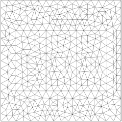
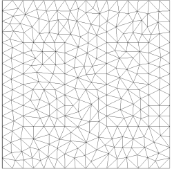
Figure 1. Domain $\Omega$ and supports $Q^{+}$, $Q^{c}$, and $Q^{-}$ for Test Case 1, together with the unrefined initial meshes. From the left to the right: Mesh 1 (constrained Delaunay, 438 nodes and 810 elements), and Mesh 2 (constrained Delaunay, 297 nodes and 528 elements). The edges of Mesh 1 are aligned with the supports of $f$ and $\mu^{*}(f)$. Mesh 2 is aligned only with the supports of $f$.

In this first set of tests we consider a square domain in $\mbox{\NUMBERS R}^{2}$, $\Omega=[0,1]\times[0,1]$, and a zero-mean forcing function $f$ supported in two rectangles $Q^{+}$ and $Q^{-}$ contained in $\Omega$, where $f$ assumes opposite signs (fig. 1). The different supports are given by:

$$Q^{+}=\left[\frac{1}{8},\frac{3}{8}\right]\times\left[\frac{1}{4},\dfrac{3}{4}\right]\quad Q^{-}=\left[\frac{5}{8},\frac{7}{8}\right]\times\left[\frac{1}{4},\dfrac{3}{4}\right]$$

To test our numerical schemes we set up two problems that differ from each other by the specific choice of $f$. The first test considers a continuous forcing function $f_{1}$ with opposite sign in $Q^{+}$ and $Q^{-}$, while in the second case a piecewise constant function $f_{2}$ is used. Their expression is given by:

$$f_{1}(x,y)\ ,\ f_{2}(x,y)=\left\{\begin{aligned} &2\sin\left(4\pi x\!-\!\frac{\pi}{2}\right)\sin\left(2\pi y\!-\!\frac{\pi}{2}\right)\ ,\ &&\quad 2\quad\mbox{ in }Q^{+}\\ -&2\sin\left(4\pi x\!-\!\frac{5}{2}\right)\sin\left(2\pi y\!-\!\frac{\pi}{2}\right)\ ,\ &&-2\quad\mbox{ in }Q^{-}\\ &0,0\quad\mbox{elsewhere}\end{aligned}\right.$$

From Buttazzo and Stepanov [12] we derive explicit formulas for the OT  density $\mu^{*}(f_{1})$ and $\mu^{*}(f_{2})$ together with their support given by $Q^{\mu}=Q^{+}\cup Q^{-}\cup Q^{c}$ with $Q^{c}=[3/8,5/8]\times[1/4,3/4]$. With this explicit solution, we can verify the experimental convergence rates at large times for the different proposed schemes. We use two different initial triangulation settings (Mesh 1 and Mesh 2, see fig. 1), each uniformly refined four times to yield four refinement levels. Both meshes are constrained to be aligned with the exact supports of $f^{+}$ and $f^{-}$, so that the condition $\sum_{i}\int_{\Omega}f(x)\varphi_{i}{}\,dx=0$ can be imposed exactly, and, at each level, have approximately the same number of nodes and elements. Mesh 1 (fig. 1, left) is a constrained Delaunay triangulations with edges aligned with the boundary of $Q^{\mu}$. Mesh 2 is also a constrained Delaunay triangulation but is not aligned with $Q^{\mu}$ in the area between $Q^{+}$ and $Q^{-}$. In the latter case, we expect convergence to be influenced also by the geometric error in approximating the boundaries of the support $Q^{\mu}$ of $\mu^{*}$. Sensitivity to initial conditions is tested by employing the following different initial data $\mu_{0}^{(i)}$:

$$\mu^{(1)}_{0}\equiv 1;\mu^{(2)}_{0}(x,y)=0.1+4|x-0.5,y-0.5\|^{2};$$

$$\mu^{(3)}_{0}(x,y)=3+2\sin(8\pi x)\sin(8\pi y).$$

Note that in these tests we do not focus on computational speed, but only on the numerical behavior of the schemes. Thus we do not limit the minimum time step size and the maximum number of iterations (in both time-stepping and the PCG algorithm used to solve the linear system of algebraic equations), and use tight tolerances to determine when time equilibrium is reached and termination of linear and nonlinear iteration: $\tau_{\mbox{{\scriptsize NL}}}=10^{-11}$ and $\tau_{\mbox{{\scriptsize T}}}=5\times 10^{-9}$, $\tau_{\mbox{{\scriptsize CG}}}=10^{-13}$. In the simulations presented here we adopt both for the forward and backward Euler time-stepping and vary the time step size by setting $\Delta t_{k+1}=\min(1.05\times\Delta t_{k},\Delta t_{\mbox{{\scriptsize max}}})$, where $\Delta t_{\mbox{{\scriptsize max}}}=0.5$. Preliminary experiments are used to calibrate this strategy so that it ensures the stability of the forward Euler scheme, or equivalently, the convergence of the Picard iteration. Convergence as $h\rightarrow 0$ is explored by looking also at the time behavior of the $L^{2}(\Omega)$ relative $\mu$-error defined as:

$$E_{\mu^{*}}(\mu):=\|\mu-\mu^{*}(f)\|_{L^{2}(\Omega)}\ /\ \|\mu^{*}(f)\|_{L^{2}(\Omega)}.$$

Convergence toward steady-state equilibrium

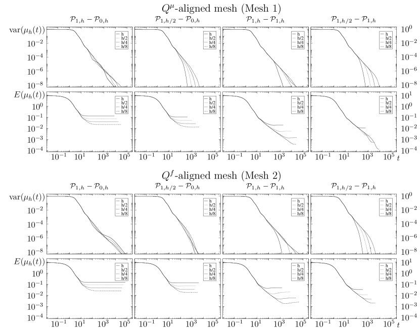
Figure 2. Convergence toward equilibrium in the case of continuous forcing ($f=f_{1}$). The log-log plots of $\operatorname{var}(\mu_{h}(t,\cdot))$ and $E_{\mu^{*}}(\mu_{h}(t,\cdot))$ vs. time are reported for Mesh 1 ($Q^{\mu}$-aligned, top block) and for Mesh 2 ($Q^{f}$-aligned, bottom block). The columns refer from left to right to the results obtained with $\mathcal{P}_{1,h}-\mathcal{P}_{0,h}$, $\mathcal{P}_{1,h/2}-\mathcal{P}_{0,h}$, $\mathcal{P}_{1,h}-\mathcal{P}_{1,h}$, $\mathcal{P}_{1,h/2}-\mathcal{P}_{1,h}$, respectively.

Figure 2 reports the log-log scale plots of $\operatorname{var}(\mu_{h}(t))$ and $E_{\mu^{*}}(\mu_{h}(t))$ vs. time, calculated for the two mesh families in the case of continuous forcing function $f_{1}$. Each curve in each sub-plot corresponds to a different mesh level. The columns are related to different combinations of spatial discretizations. Only results of the Explicit Euler time-stepping scheme are shown, the results of the Implicit Euler method being identical. The first set of plots (first two rows) are relative to the $Q^{\mu}$-aligned mesh set, while the lower set reports the results for the $Q^{f}$-aligned meshes.

The results show a steady convergence toward the equilibrium point $\mu_{h}^{*}$. The $\mu_{h}$ variation, $\operatorname{var}(\mu_{h}(t))$, displays a monotone behavior for all schemes, with an expected geometric convergence rate toward steady-state, as evidenced by the slope of the rectilinear portions of the curves that coincides for all mesh levels and types. At increasing refinement levels the convergence curves have a common initial behavior for all schemes but start to diverge approximately when the corresponding spatial accuracy limit is attained. Accuracy saturation in the error plots ($E_{\mu^{*}}(\mu_{h}(t))$ vs. $t$) occurs at the same time at which $\operatorname{var}(\mu_{h}(t))$ start diverging. More uncertain profiles are obtained when spatial discretization is performed on the same mesh for the pair $(\mu_{h},u_{h})$ for both $\mathcal{P}_{1}-\mathcal{P}_{0}$ and $\mathcal{P}_{1}-\mathcal{P}_{1}$ discretization spaces. The reason for the loss of regularity is to be attributed to oscillations in the cell gradients that cause amplified oscillations in the corresponding transport density. Spatial averaging of the gradient magnitudes, leading to the $\mathcal{T}_{h}-\mathcal{T}_{h/2}$ formulation, shows a much smoother behavior with a faster convergence towards equilibrium. We postpone a more detailed discussion of this phenomenon to section 4.2, where a more challenging test case is approached.

Looking at the bottom half of fig. 2, we see the effect of using meshes that are not aligned with the support of the optimal transport density. Because of the discontinuity in $\mu_{h}$ occurring across the boundary of $Q^{\mu}$, convergence is limited by the geometric convergence of the triangular shapes towards this boundary, and the global attainable accuracy is bounded by this error. We observe a consistent behavior of the error for both mesh-types at different $h$ levels. The accuracy levels at which the error saturates decrease consistently with the expected order of spatial convergence of the different schemes, when the geometric error is negligible. This is clearly observable by looking at the plots of $\operatorname{var}(\mu_{h}(t))$ for the $\mathcal{P}_{1,h/2}-\mathcal{P}_{0,h}$, and the $\mathcal{P}_{1,h/2}-\mathcal{P}_{1,h}$, cases, where the optimal second order convergence of the latter approach is observable from the fact that difference in the attained accuracy levels are doubled with respect to the first order approach. Higher order methods display higher accuracy, but the geometric error prevents the realization of optimal convergence rates.

Convergence of the spatial discretization

Figure 3. Behavior of $E_{\mu^{*}}(\mu_{h}^{*})$ vs. $h$ for the different discretization methods. The results for the continuous forcing function $f_{1}$ are shown in the left column, while the right column reports the results for $f_{2}$. The top row is relative to the Mesh-1 sequence (aligned with $Q^{\mu}$), while the bottom row corresponds to the Mesh-2 sequence (aligned only with $Q^{f}$). For visual reference, the first order convergence line is also plotted with a thick solid trait. The average experimental convergence rates are reported in the legends of each plot next to the discretization method.

  

  

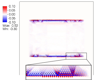
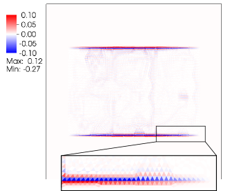
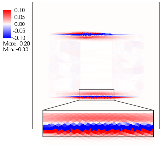
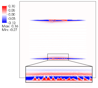
Figure 4. Spatial distribution of the error $\mu_{h}^{*}-\mu^{*}(f_{2})$ at steady state for the piecewise constant forcing function $f_{2}$. The upper row reports the results on the finest level of Mesh-1 obtained with the $\mathcal{P}_{1,h}-\mathcal{P}_{0,h}$, (left) and $\mathcal{P}_{1,h}-\mathcal{P}_{1,h}$, (right). The lower row shows the results on the finest level of Mesh-2 from the $\mathcal{P}_{1,h/2}-\mathcal{P}_{0,h}$, (left) and $\mathcal{P}_{1,h/2}-\mathcal{P}_{1,h}$, (right) approaches.

We would like to recall that continuity of the transport density $\mu^{*}(f)$ when the forcing term $f$ is continuous was proved in $\mbox{\NUMBERS R}^{2}$ in Fragalà et al. [21] under some assumptions on $f$. However, except for partial regularity results along transport rays [12], the general case seems to be an open question. In our test cases, for both $f_{1}$ and $f_{2}$ forcings, strong variations in $\mu_{h}$ are present in a direction orthogonal to the boundary of $Q^{\mu}$ in the central portion of the domain (outside $Q^{f}$). Because of these variations, which in the discontinuous forcing case are actual $\mu^{*}$-discontinuities, we expect a loss of convergence in the FE solution. We note, however, that convergence towards steady-state is not influenced by spatial errors, as shown in the previous discussion.

The experimental convergence profiles for the different methods are reported in fig. 3. The column on the left groups the results relative to the more regular case of continuous forcing function $f_{1}$. The right column reports the results obtained for piecewise constant forcing $f_{2}$. The top and bottom rows identify the mesh sequences aligned with the boundary of $Q^{\mu}$ or with the boundary of $Q^{f}$, respectively.

From the two plots on the left, we can argue that: i) all methods attain optimal convergence when the Mesh-1 sequence is used; ii) the $\mathcal{T}_{h}-\mathcal{T}_{h/2}$ combination is characterized by a smoother behavior; iii) the use of the Mesh-2 sequence, which we recall is aligned only with the boundaries of $Q^{f}$ and not those of $Q^{\mu}$, triggers the emergence of geometrical errors that cause a sizeable reduction on the convergence rates of both $\mathcal{P}_{1}-\mathcal{P}_{1}$ and $\mathcal{P}_{1}-\mathcal{P}_{0}$ schemes.

As expected, the results for the discontinuous forcing function (right column) are characterized by an important loss of convergence rate for all schemes, except the $\mathcal{P}_{1,h/2}-\mathcal{P}_{0,h}$ in combination with the $Q^{\mu}$-aligned meshes. The use of a $\mathcal{T}_{h}-\mathcal{T}_{h/2}$ combination seems to be more robust. This is confirmed by the spatial distribution of the error $\mu_{h}^{*}-\mu^{*}(f_{2})$ shown in fig. 4. In this figure we report the results obtained with the $\mathcal{P}_{1,h}-\mathcal{P}_{0,h}$ (upper left panel) and the $\mathcal{P}_{1,h}-\mathcal{P}_{1,h}$ (upper right panel) for Mesh 1, and the $\mathcal{P}_{1,h/2}-\mathcal{P}_{0,h}$ (lower left panel) the $\mathcal{P}_{1,h/2}-\mathcal{P}_{1,h}$ (lower right panel) for Mesh 2. The plots suggest that the $\mathcal{P}_{1}-\mathcal{P}_{1}$ approach localizes the error on the north and south boundaries of $Q^{\mu}$, where the jump in $\mu^{*}$ is concentrated. The $\mathcal{P}_{1}-\mathcal{P}_{0}$ approach, on the other hand, displays an additional small but non negligible error on the support of the forcing function $Q^{f}$. The zooms on the pictures show clear oscillations for the one-mesh methods (upper row) in both directions orthogonal and parallel to the $\mu_{h}$-discontinuity. On the contrary, the methods based on two-meshes (lower row) exhibit a monotone error behavior along the boundary of $Q^{\mu}$, but the mis-alignment of the triangle edges causes an increased error as compared to the Mesh-1 results. The error slightly oscillates in the direction normal to the $\mu_{h}$-jump due to the gradient reconstruction. It is evident that the smoothing due to the averaging of the gradient magnitude on the larger triangles helps in reducing overall oscillations. This will become more evident when we will discuss in section 4.2.

Implicit Euler and convergence of the Picard scheme

In the case of implicit Euler time-stepping, the nonlinear system is solved by Picard iteration as described in LABEL:eq:p1picard. Unfortunately, the lack of a uniform bound on $|\operatorname{\nabla}u(t)|\,\forall t\geq 0$ prevents the theoretical derivation of an estimate of the contraction factor. Experimentally, all numerical experiments displayed a number of iterations of the Picard scheme increasing linearly with the time step size $\Delta t_{k}$, suggesting a fixed rate of contraction. This was evaluated by computing the relative $\mu_{h}$-variation:

$$C(k):=\frac{\|\mu_{h}^{m^{*},k}-\mu_{h}^{m^{*}-1,k}\|_{L^{2}(\Omega)}}{\|\mu_{h}^{m^{*}-1,k}-\mu_{h}^{m^{*}-2,k}\|_{L^{2}(\Omega)}}$$

where $m^{*}$ is the Picard iteration number at convergence. Independently of the spatial discretization method, preliminary numerical experiments, not reported here, showed that $C(k)\approx\Delta t_{k}$, suggesting that $\Delta t_{k}$ can be used as a proxy to control the time-step evolution in this case. Values $\Delta t_{k}\geq 1$ caused non-convergence of the Picard iteration, thus we impose an upper limit of $\Delta t_{\mbox{{\scriptsize max}}}=0.5$. This choice offered a good trade-off between minimizing the number of Picard iterations and maximizing the time-step size. At the same time, convergence of the Picard scheme was achieved with an acceptably small number of Picard iterations, averaging between 2 and 8 depending on the simulation. Because of the exponential decay of the solution in time, as predicted by the mild solution of eq. 1b, the time step size was incremented at every step by a factor 1.05.

Dynamics of $\mathcal{S}\left(\mu(t)\right)$, $W_{1}$-distance and computational cost

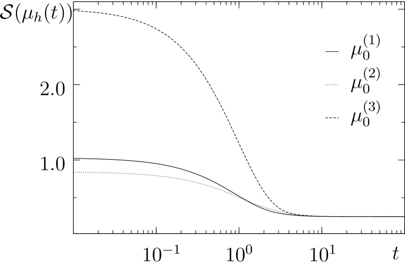
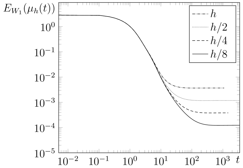
Figure 5. Test Case 2: numerical statistics for $\mathcal{P}_{1,h/2}-\mathcal{P}_{0,h}$ on Mesh 2 ($Q^{f}$ aligned). Top left panel: time behavior of the Lyapunov-candidate functional $\mathcal{S}(\mu_{h}(t))$ for three the initial data $\mu_{0}$ in LABEL:eq:initial-conditions. Bottom left panel: time behavior of $E_{W_{1}}(\mu_{h}(t))$ for four refinement levels starting with $\mu_{0}=1$. Right panel: table with simulation statistics, including # of time steps, time $(t)$, number of PCG iterations, $E_{W_{1}}(t)$, and CPU time (in seconds). Corresondingly, $\operatorname{var}(\mu_{h}(t))$ varies in the range $10^{-1}$ and $10^{-8}$.

In this paragraph we report numerical evidence of the statements in Propositions 1 and 2. We also include a discussion on computational cost to show the effectiveness of the proposed approach, although the employed numerical techniques are not optimized. In fact, a number of cost-saving strategies can be envisaged, including using coarse-mesh solutions to extrapolate initial guesses of $\mu_{0}$, re-use of stiffness and preconditioning matrices, use of a Newton-Raphson strategy to improve stability and allow for larger time-step sizes together with an inexact Krylov linear solver, etc. On the other hand, in this work we are interested in showing that, although far from optimal, our approach is potentially very effective and competitive with literature approaches in the solution of the Monge-Kantorovich equations.

Figure 5 (top-left panel) reports the time behavior of $\mathcal{S}(\mu_{h}(t))$ for the different initial conditions described in LABEL:eq:initial-conditions using the finest mesh of set 2 of the $\mathcal{P}_{1,h/2}-\mathcal{P}_{0,h}$ method. The results for other methods and mesh sets are practically indistinguishable, and are not reported here. We see that $\mathcal{S}$ decreases monotonically and always attains the same minimum value in time independently of the initial conditions. After $t\approx 100$ the value of $\mathcal{S}(\mu_{h}(t))$ becomes approximately stationary, up to machine precision.

The differences among mesh levels emerge after scaling the value of $\mathcal{S}(\mu_{h}(t))$ with its assumed asymptotic value. According to Proposition 2 this value is the minimum of the $\mathcal{S}$ and is equal to the $W_{1}$-distance between $f^{+}$ and $f^{-}$. For Test Case 2 this value is given by $0.125$, (equal to the integral of the OT  density), allowing us to compute the relative error as

$$E_{W_{1}}(\mu):=\frac{\mathcal{S}(\mu)-0.125}{0.125}.$$

The bottom left panel in fig. 5 reports the time-evolution of $E_{W_{1}}(\mu_{h}(t))$ for four mesh refinements. Similarly to the behavior of $\operatorname{var}(\mu_{h}(t)$ in fig. 2, $E_{W_{1}}(\mu_{h}(t))$ shares the same profile for all mesh levels until $t\approx 10$. At this time the graphs start separating and converge to their corresponding asymptotic values that scale approximately linearly with $h$. This implies that the stop-tolerance $\tau_{\mbox{{\scriptsize T}}}$ used to identify steady state can be relaxed depending on the sought accuracy. In fact, two distinct phases can be identified. The first initial phase displays profiles of $\operatorname{var}(\mu_{h}^{k})$, $E_{\mu^{*}}(\mu_{h}^{k})$, and $E_{W_{1}}(\mu_{h}(t))$ that are superimposed and independent of the mesh level. This phase is characterized by strong variations of $\mu_{h}$, and consequently, by higher number of PCG iterations. After this initial phase, $\mu_{h}$ varies more slowly and stabilizes within $Q^{\mu}$ to its final value which depends upon the actual mesh size. At the same time, in $\Omega\setminus Q^{\mu}$, the decay continues towards zero. This phase is characterized by larger time-step sizes and faster PCG convergence, but much slower convergence of $\mu_{h}$ to its asymptotic value, so that only marginal accuracy gains require large computational efforts. The use of increasingly refined meshes should be able to exploit the iterative process of the DMK approach with consistent reduction of the computational cost.

These results suggest that the proposed approach can be very efficient in evaluating $W_{1}$ distances. This statement is corroborated by the computational statistics collected in the table shown in the right panel of fig. 5. For the four mesh levels, we show simulation time ($t$), cumulated number of time steps ($\#it$), number of linear (PCG) iterations, the value of $E_{W_{1}}(\mu_{h}(t))$, and CPU time in seconds. The data reported are collected during the simulation at each change in order of magnitude of $\operatorname{var}(\mu_{h}(t))$ in the range $10^{-1}$ to $10^{-8}$. The runs are conducted on a 3.4GHz Intel-I7 (1-core) computer. The table shows that $h$ determines the practical bound of achievable accuracy in the evaluation of the $W_{1}$ distance. For example, looking at the results for $\mathcal{T}{h/4}$, it evidently useless go beyond $t=405$, at which time the accuracy in the $W_{1}$ distance is already $4.6\cdot 10^{-5}$, not far from the highest achievable error accuracy of $4\cdot 10^{-5}$. Note that with $\mathcal{T}{h}$ at $t=60.4$ which achieve an accuracy of $3.7\cdot 10^{-3}$ with a mere 1.2 seconds of CPU time. Most of this error is probably due to the geometric error of having a mesh not aligned with the support of the OT  density.

4.2. Test Case 2: comparison with literature and stability of the spatial discretization

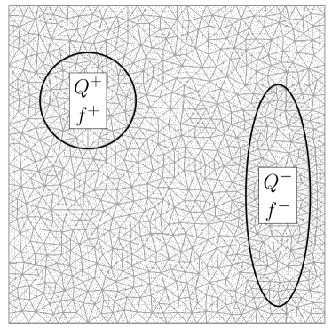
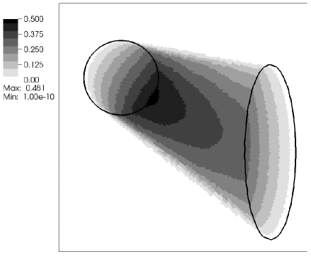
Figure 6. Domain and supports of the forcing function used in the discretization of the MK equations eq. 2 for the solution of Example 1 of Barrett and Prigozhin [1]. The two triangulations $\mathcal{T}_{h}$ and $\mathcal{T}_{h/2}$ are shown with blue and dashed black lines, respectively.

In this section we address a test case proposed by Barrett and Prigozhin [1]. The problem considers the transport of a uniform density supported on a circle towards a disjoint ellipsis. Figure 6 (left) shows the domain $\Omega$ where problem eq. 2 is defined and the supports $Q^{+}$ and $Q^{-}$ of the forcing term $f=f^{+}-f^{-}$, with $f^{+}(x)=2$ for $x\in Q^{+}$ and zero otherwise, and $f^{-}(y)$, appropriately rescaled for $y\in Q^{-}$ to ensure mass balance. The coarse initial mesh is also shown in light blue lines, and its uniform refinement is shown in thin dashed lines. This mesh, characterized by 820 nodes and 1531 triangles, is a constrained Delaunay triangulation that follows the boundaries of both $Q^{+}$ and $Q^{-}$. The same Figure shows in the right panel the time-converged spatial distribution of the transport density numerically evaluated with the most stable discretization method, $\mathcal{P}_{1,h/2}-\mathcal{P}_{0,h}$, on the finest mesh. The spatial distribution of $\mu_{h}$ is in good agreement with the results obtained by Barrett and Prigozhin [1], achieving its maximum value (0.482) on the boundary of the left circle, and its minimum value $10^{-10}$ set by the prescribed lower bound as discussed in section 3.3. This solution is used in the following digression as a reference solution. We would like to note that a similar test case was already proposed in Facca et al. [18] to to test the conjecture that the solution of the dynamic MK problem eq. 2 converges at infinite time towards the solution of the static MK equations. In this section we re-use this example to experimentally discuss the need to use different FEM spaces for the discretization of the transport density and of the transport potential.

   

   

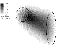
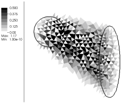
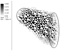
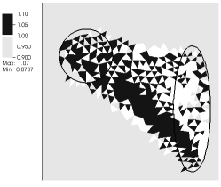
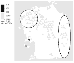
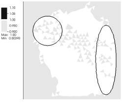
Figure 7. Solution of Test Case 2 at $t_{1}=2.73\times 10^{2}$ (left), $t_{2}=1.36\times 10^{3}$(center) , and $t_{3}=2.5\times 10^{5}$(right), using the $\mathcal{P}_{1,h}-\mathcal{P}_{0,h}$ approach. Top row: spatial distribution of $\mu_{h}\in\mathcal{P}_{0,h}$. Bottom row: spatial distribution of $|\operatorname{\nabla}u_{h}|\in\mathcal{P}_{0,h}$ as calculated from $u_{h}\in\mathcal{P}_{1,h}$.

We start this discussion by presenting the results obtained using the $\mathcal{P}_{1,h}-\mathcal{P}_{0,h}$ approach on the coarsest grid and look at three different times during the evolution. The times are selected so that $\operatorname{var}(\mu_{h}^{k})$ reaches the values $10^{-3}$, $10^{-4}$, $5\times 10^{-8}$, namely $t_{1}=2.73\times 10^{2}$, $t_{2}=1.36\times 10^{3}$, and $t_{3}=2.5\times 10^{5}$, the latter time corresponding to the time-converged solution. We plot in fig. 7 both $\mu_{h}$ (upper panels) and $|\operatorname{\nabla}u_{h}|$ (lower panels).

At the first sampled time the solution clearly resembles the reference solution shown in fig. 6 (right), although at a much coarser resolution. The corresponding gradient (shown in the second row) displays some slight but acceptable overshoots in a region that resembles $Q^{\mu}$. Already at this early time, which occurs after 1630 time steps, some oscillations are visible. At time $t_{2}$ these oscillations are much more pronounced with a checkerboard pattern that suggests an intrinsic instability of the scheme. We should note that the color scale in the plots are limited from above and from below by suitable values to emphasize the oscillations. The maximum and minimum values for both $\mu_{h}$ and $|\operatorname{\nabla}u_{h}|$ are reported right below each legend. We observe that there are no overshoots in $|\operatorname{\nabla}u_{h}|$, which at the final time is never greater than one. Still, checkerboard-like fluctuations are visible, causing the dynamic equation to drive $\mu_{h}$ to zero quickly thus determining a drastic deterioration of the solution accuracy.

   

   

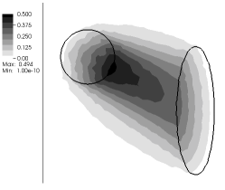
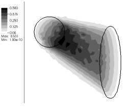
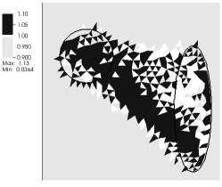
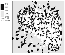
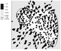
Figure 8. Solution of Test Case 2 at $t_{1}=6.82^{1}$ (left), $t_{2}=5.36^{2}$ (center), and $t_{3}=9.65time10^{3}$ (left), using the $\mathcal{P}_{1,h}-\mathcal{P}_{1,h}$ approach. Top row: spatial distribution of $\mu_{h}\in\mathcal{P}_{1,h}$. Bottom row: spatial distribution of $|\operatorname{\nabla}u_{h}|\in\mathcal{P}_{0,h}$ calculated from $u_{h}\in\mathcal{P}_{1,h}$.

The situation does not improve by using higher order spaces for $\mu_{h}$. Figure 8 shows the results obtained by using a $\mathcal{P}_{1,h}-\mathcal{P}_{1,h}$ approach. We still observe oscillations, albeit appearing at a later time and with a different pattern. Once oscillations in $|\operatorname{\nabla}u_{h}|$ around the unit value start developing, the dynamic equation determines a decay of $\mu_{h}$ within the elements where $|\operatorname{\nabla}u_{h}|<1$ even if located within $Q^{\mu}$. This decay quickly reinforces in time leading to the observed checkerboard pattern. The behavior resembles the classical lack of stability due to a violation of an inf-sup-like constraint, but at this point we are not able to clearly identify this condition.

   

   

   

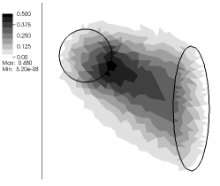
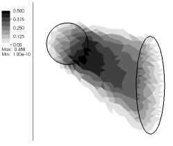
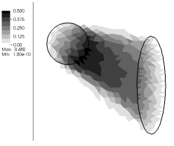
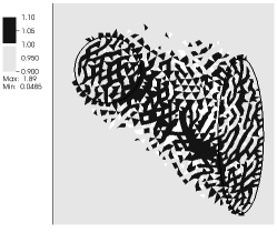
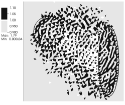
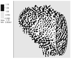
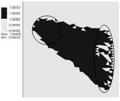
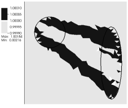
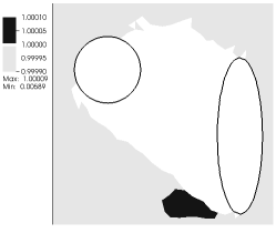
Figure 9. Solution of Test Case 2 at $t_{1}=6.75\times 10^{1}$ (left), $t_{2}=2.04\times 10^{2}$ (center), and $t_{3}=1.54\times 10^{3}$ (right) using the $\mathcal{P}_{1,h/2}-\mathcal{P}_{0,h}$ approach. Top row: spatial distribution of $\mu_{h}\in\mathcal{P}_{0,h}$. Middle row: spatial distribution of $|\operatorname{\nabla}u_{h}|\in\mathcal{P}_{0,h/2}$ calculated from $u_{h}\in\mathcal{P}_{1,h/2}$. Bottom row: spatial distribution of $|\operatorname{\nabla}u_{h}|\in\mathcal{P}_{0,h}$.

On the other hand, oscillations completely disappear if we employ a two-mesh approach. Looking at the checkerboard oscillations displayed in fig. 7, it is intuitive to think that averaging the gradient magnitude between neighboring triangles should compensate the fluctuations. This observation led us to employ the $\mathcal{P}_{1,h/2}-\mathcal{P}_{0,h}$ discretization described in section 3. Indeed, with this approach the gradients calculated from $u_{h}\in\mathcal{P}_{1}(\mathcal{T}_{h/2})$ are projected onto the space $\mathcal{P}_{0}(\mathcal{T}_{h})$ for insertion into the dynamic equation eq. 8b. This projection is equivalent to averaging the piecewise constant gradients over the four triangles of $\mathcal{T}_{h/2}$ that form one triangle of $\mathcal{T}_{h}$. This results in a oscillation free $\mu_{h}$ field, as shown in fig. 9. It is evident that no $\mu_{h}$ oscillations form even at the coarsest mesh level used in this test. Note that the spatial discretization of the elliptic equation does not guarantee monotonicity [26]. In fact, the gradient magnitudes arising from $u_{h}\in\mathcal{P}_{1,h/2}$ still show the classical checkerboard fluctuations (fig. 9, middle row). However, the projection of $|\operatorname{\nabla}u_{h}|$ onto $\mathcal{P}_{0,h}$ (fig. 9, bottom row) does not show oscillations, albeit small overshooting occurs especially at the earlier times. We should emphasize that $|\operatorname{\nabla}u_{h}|$ is plotted here using an extremely narrow color scale ranging within $[0.9999,1.0001]$.

Looking at the final time-converged solution, the value $|\operatorname{\nabla}u_{h}^{*}|$ within the support of $\mu_{h}^{*}$ and neighboring regions is exactly unitary, and remains bounded by 1 almost everywhere, in compliance with the constraint of the MK equations. Only one small region with $|\operatorname{\nabla}u_{h}^{*}|>1$ develop with a maximum value approaching 1.00009, considered consistent with the tolerance used in the PCG linear solve. Indeed, oscillations of the order of $10^{-5}$ in the gradient magnitude may be indistinguishable by the linear solver of the $u_{h}$ equation. Similar considerations can be done in the case $\mu_{h}\in\mathcal{P}_{1,h}$ (not shown here) but in this case some oscillations in $|\operatorname{\nabla}u_{h}|$ persist even when $u_{h}\in\mathcal{P}_{1,h/2}$. This reinforces the conjecture that some sort of inf-sup stability condition exists that couples the discretization spaces for $u_{h}$ and $\mu_{h}$, and will be the subject of further studies.

One final observation for this test case concerns the computational cost of our approach. In comparison with the technique proposed by Barrett and Prigozhin [1], our method seems to be computationally advantageous. In fact, as already mentioned, the simulations reported in Barrett and Prigozhin [1] where obtained using a mixed FEM approach in combination with adaptive mesh refinement, leading to nonlinear systems of dimension approaching 60000. In our case, the dimensions for the smallest test case are 1531 (number of triangles in $\mathcal{T}_{h}$) and 3170 (number of nodes in $\mathcal{T}_{h/2}$) for the diagonal dynamic algebraic system and the elliptic system, respectively, leading to a total of 4701 degrees of freedom. Note that the finest solution of fig. 6 was obtained with a total of 73917 degrees of freedom. Our confidence that the approach we propose is superior to that Barrett and Prigozhin [1] is is reinforced by the observation that effective simulations can be obtained at intermediate mesh levels. Moreover, time-convergence can be considered achieved at much earlier times then the ones employed in this work if we look at the stationarity of the Lyapunov-candidate functional. Obviously, adding simple adaptive mesh refinement strategies would greatly enhance the performance of the studied methodology.

4.3. Test case 3: $L^{1}$-Optimal Transport map

In this section, we present a further experiment where the numerical solution $(\mu_{h}^{*},u_{h}^{*})$ from the DMK approach is used to compute approximate $L^{1}$-OT Maps following the algorithm suggested in Evans and Gangbo [17]. Finally, these results are compared with approximate maps obtained by linear programming or the Sinkhorn algorithm with entropic regularization [25].

This experiment is shaped after Li et al. [23], and considers a square domain $\Omega=[0,1]\times[0,1]$ with a source term $f^{+}$ supported in the ball of radius $0.35$ centered and $(x_{c},y_{c})=(0.5,0.5)$ given by $f^{+}(x,y)=max(0,1-\sqrt{(x-x_{c})^{2}+(y-y_{c})^{2}})$. The sink term $f^{-}$ is the sum of four functions of the same form of $f^{+}$, but located near the four corners of the domain. All the terms are balanced to ensure zero mean of $f$. The problem setting together with the triangulation used in the DMK solution is shown in fig. 10. Note that in this test case the OT map will necessarily split $f^{+}$ into four different subsets that are reallocated towards the four disjoint sinks $f^{-}$. The resulting singular distribution poses non trivial issues on the numerical solution of the problem.

Calculation of the OT map via DMK

Given two Lipschitz continuous forcings $f^{+}$ and $f^{-}$ with disjoint supports, the OT map $T^{*}:\mbox{supp}(f^{+})\mapsto\mbox{supp}(f^{-})$ can be defined as $T^{*}(x):=z(1,x)$, where $z(t,x)$ is the solution of the following Cauchy Problem [17]:

(11) $$\left\{\begin{aligned} z^{\prime}(t)&=Y(t,z(t))\\ z(0)&=x\in Q^{+}\end{aligned}\right.\quad Y(t,z)=\frac{-\mu^{*}\operatorname{\nabla}u^{*}}{(1-t)f^{+}(z)+tf^{-}(z)}.$$

Thus, we first compute $(\mu_{h}^{*},u_{h}^{*})$ via the $\mathcal{P}_{1,h/2}-\mathcal{P}_{0,h}$ approach combined, for simplicity, with Explicit Euler time-stepping. We adopt the same parameters (time step, linear solver tolerance, stop criteria, etc.) used in the other experimental tests in this paper. Then, we construct the approximate OT map by evaluating the streamlines of the vector field $Y$ in eq. 11 emanating from the barycenters of the triangles discretizing the support of $f^{+}$. In order to avoid division by zero in eq. 11, we replace the term $(1-t)f^{+}(z)+tf^{-}(z)$ with $min[(1-t)f^{+}(z)+tf^{-}(z)],10^{-5}]$. Time-integration is performed with a 4-th order Runge-Kutta method. We denote with $T^{*}_{h}(DMK)$ this approximate OT map.

Calculation of OT map via barycentric map

The second method considered follows the approach detailed in Perrot et al. [25], where an approximate OT map is built from an approximate OT plan. First, $f^{+}$ and $f^{-}$ are discretized with two atomic measures $\underline{f}^{+}$ and $\underline{f}^{-}$:

(12) $$\underline{f}^{+}=\sum_{i=1}^{N_{+}}{s}_{i}\delta(\bar{x}_{i})\quad\underline{f}^{-}=\sum_{j=1}^{N_{-}}{t}_{j}\delta(\bar{y}_{j}),$$

where $(\bar{x}_{i})_{i=1,\ldots,N_{+}}$ and $(\bar{y}_{j})_{i=1,\ldots,N_{-}}$ are sampling points in the support of $f^{+}$ and $f^{-}$. We then denote with $\boldsymbol{\gamma^{*}}$ the solution of the Linear Programming problem solving the classical $L^{1}$-OTP given $\underline{f}^{+},\underline{f}^{-}$. The associated barycentric map $T^{*}[\gamma^{*}]$ is defined as:

(13) $$T^{*}[\boldsymbol{\gamma^{*}}](\bar{x}_{i}):=\operatornamewithlimits{argmin\vphantom{q}}_{y\in\Omega}\sum_{j=1}^{N_{-}}{\gamma^{*}}_{i,j}\ |y-\bar{y}_{j}|\quad\forall i=1,\ldots,N_{+}.$$

In order to build the approximate OT map that can then be compared with $T^{*}(DMK)$, the sampling points $(\bar{x}_{i})_{i=1,\ldots,N_{+}}$ and $(\bar{y}_{j})_{i=1,\ldots,N_{-}}$ are taken to be the barycenters of the triangles discretizing the support of $f^{+}$ and $f^{-}$, respectively. The coefficients $\underline{s}\in\mbox{\NUMBERS R}^{N_{+}}$ and $\underline{t}\in\mbox{\NUMBERS R}^{N_{-}}$ in eq. 12 are then computed as:

$${s}_{i}=\int_{T_{i}}f^{+}\,dx\quad\forall T_{i}\in\mbox{supp}(f^{+})\qquad{t}_{j}=\int_{T_{j}}f^{-}\,dx\quad\forall T_{j}\in\mbox{supp}(f^{-}).$$

We use two algorithms contained in the POT toolbox [20] to find the OT Plan $\boldsymbol{\gamma^{*}}$ for the discrete OTP. The first algorithm is based on a classical LP solver and we denote with $\boldsymbol{\gamma^{*}_{h}}$, this approximated OT plan. The second algorithm is based on the the Sinkhorn regularization of discrete $L^{1}$-OTPdescribed in Cuturi [14]. We denote with $\boldsymbol{\gamma^{*}_{h,\varepsilon}}$ its approximate solution, where $\varepsilon$ indicates the Sinkhorn relaxation parameter with value $\varepsilon=8e-4$, which was experimentally evaluated to avoid algorithm failure. The barycentric maps of the two plan are given by:

$$T^{*}(LP):=T^{*}[\boldsymbol{\gamma^{*}_{h}}]\quad T^{*}(S):=T^{*}[\boldsymbol{\gamma^{*}_{h,\varepsilon}}].$$

The computation of $T^{*}(LP)$ and $T^{*}(S)$ requires the solution of eq. 13, i.e., a weighted version of the Fermat-Weber location problem, solved in our case with the algorithm described in Vardi and Zhang [30].

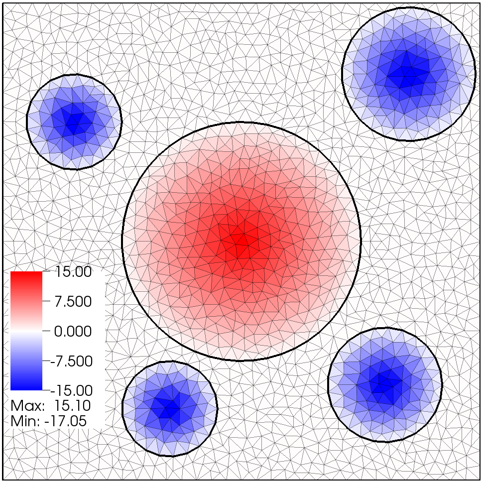
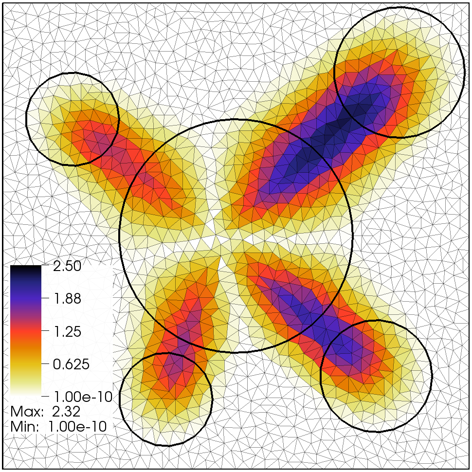
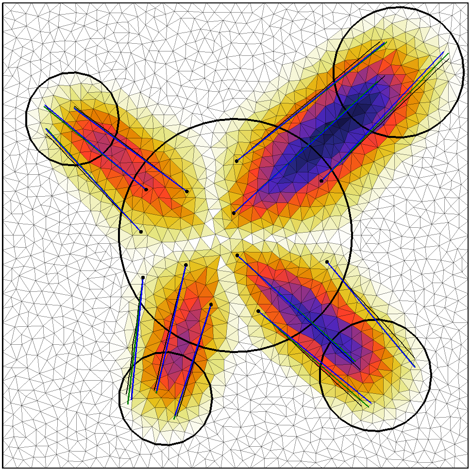
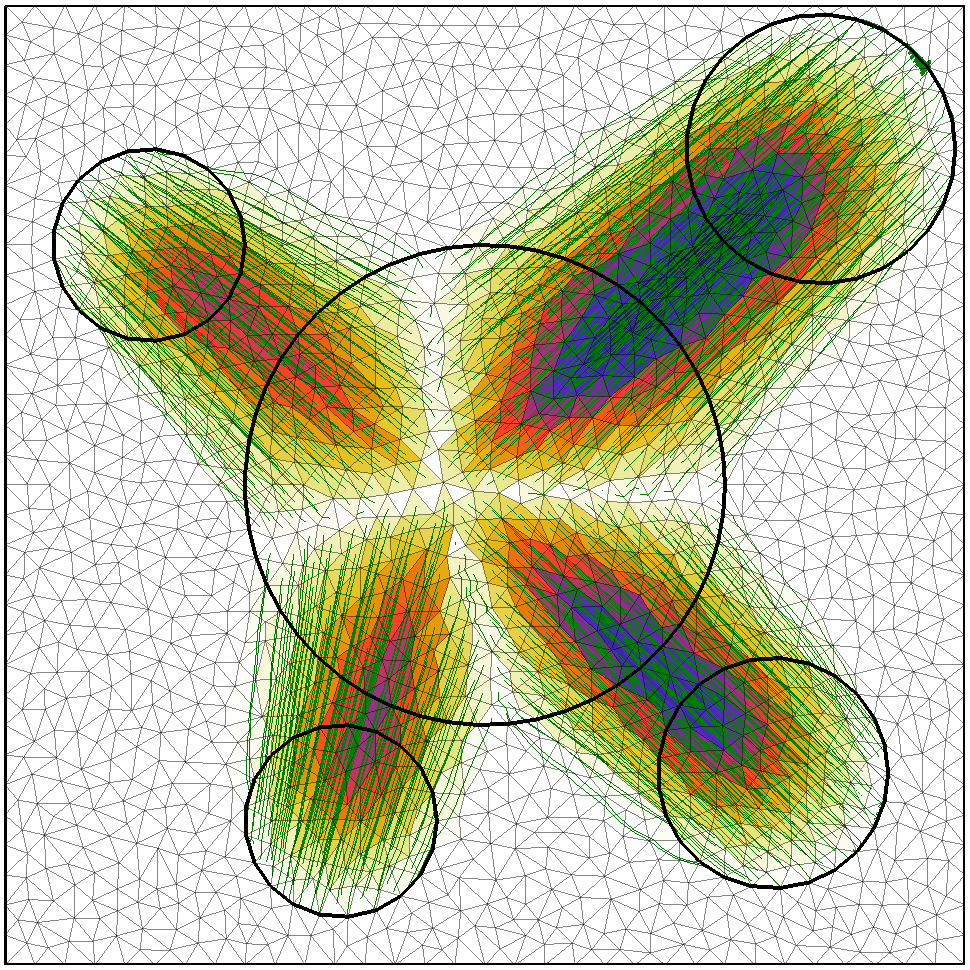
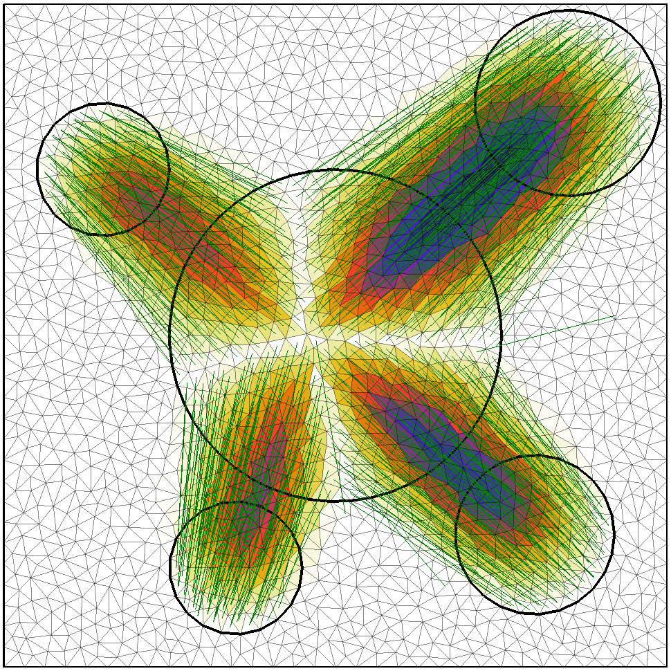
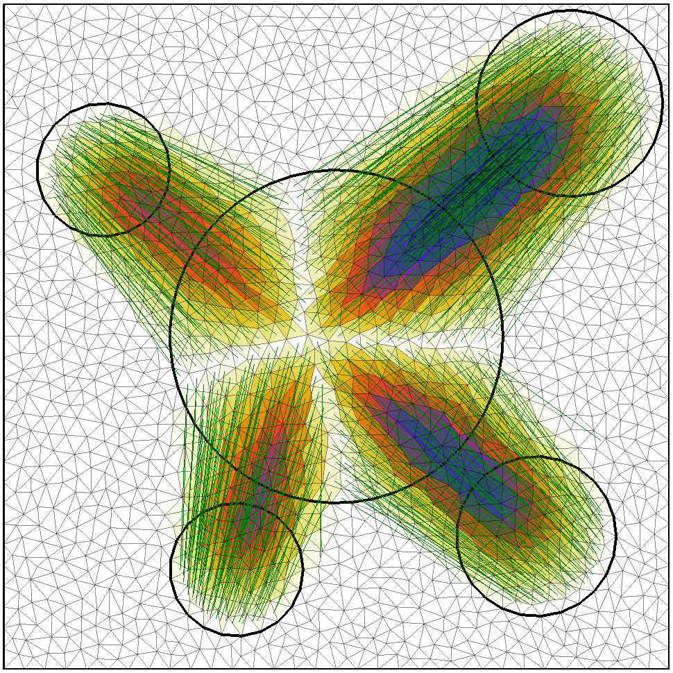
Figure 10. Test case 3. The top row contains the problem definition with the triangulation $\mathcal{T}_{h}$ ($1699$ nodes and $3265$ triangles) used in the solution of DMK, the source (red) and the sink(blue) terms (left); the approximate OT density $\mu_{h}^{*}$ distribution obtained via DMK (middle) and the comparison between OT maps calculated with DMK, LP, and Sinkhorn algorithms for few barycenters. The bottom row contains the full OT maps calculated starting from the triangle barycenters by the DMK (left), the LP (middle), and the Sinkhorn (right) algorithms.

The spatial distribution of $\mu_{h}^{*}$ as calculated by the DMK approach is shown in the top central panel in fig. 10. We note the four regions into which the support of $f^{+}$ is divided. Each region corresponds to the “portion” of $f^{+}$ that is sent to each one of the four circles where $f^{-}$ is supported. We call $\Gamma$ the one-dimensional boundary dividing these regions. In the right top panel we compare the lines connecting 12 sampling point in $\mbox{supp}(f^{+})$ with their image through the maps $T^{*}(DMK)$ (black), $T^{*}(LP)$ (green) and $T^{*}(S)$ (blue). The three approximated maps are qualitatively similar, suggesting that $\mu_{h}^{*}$ can be effectively used to determine transport maps. The bottom panels of fig. 10 show the full OT maps calculated for triangle barycenters within $\mbox{supp}(f^{+})$ with the three considered methods. We first note the almost prefect coincidence of the supports of these lines with the support of $\mu_{h}^{*}$. Almost all the streamline computed for the map $T^{*}_{h}(DMK)$ are perfectly straight, with the end-points on the lines covering $\mbox{supp}(f^{-})$. The computation of the optimal destination of the barycenters close to $\Gamma$ creates some numerical difficulties for all methods. Indeed, the image of the $T^{*}_{h}(LP)$ and $T^{*}_{h}(S)$ with domain located in barycenters of triangles located in $\Gamma$ fall outside $\mbox{supp}(f^{-})$. For $T^{*}_{h}(DMK)$, some of the streamlines starting from these points are not exactly straight, while others remain stack at the starting point. Mesh refinement around $\Gamma$ should help to give a better characterization the partitions dividing $\mbox{supp}(f^{+})$. In the DMK model this mesh refinement strategy is easily accomplished as triangles to be refined are easily identified by the fact that $\mu_{h}^{*}$ tends to zero in the $\mbox{supp}(f^{+})$. Another advantage of the DMK method is that, given a new sample point $\bar{x}\in\mbox{supp}(f^{+})$, we can compute $T^{*}_{h}(\bar{x})$ without recomputing the pair $(\mu_{h}^{*},u_{h}^{*})$. The computational effort required is only the integration of the Cauchy Problem eq. 11. The results of this test case show that, for this case of $L^{1}$-OTP, our approach does not suffer of the out-of samples problem described in Perrot et al. [25].

5. Conclusions

The performance of the proposed finite element method for the solution of the dynamic Monge-Kantorovich equations has been thoroughly analyzed experimentally on several test cases. The results show that the strategy for solving the MK equations by searching for the stationary solution of the dynamic MK problem is highly promising. These experiments show that the resulting discrete system achieves optimal convergence in space and time even when using simple successive (Picard) linearization schemes.

The enhancement path for the proposed approach is clear. Some of the issues currently under study include the development of a Newton method for the solution of the nonlinear system in the case of implicit Euler time-stepping, to completely exploit the geometric convergence towards steady state only hinted at in the present paper. Further improvements can be readily obtained by careful use of a sequence of meshes with progressively finer resolution as time increases, with adaptation to the support of the transport density easily achievable. The iterative nature of DMK approach allows the tight control of these computational savings both in the spatial and in the time discretizations.

Theoretical work is needed to ascertain the formal convergence of the proposed methods and to determine the exact relationships between the spatial discretization spaces used for $u_{h}$ and $\mu_{h}$ that guarantee stability of the approach. Future studies include the handling of less regular forcing functions to address the more interesting problems that can be studied by means of Optimal Transport theory. We believe that this work can be a useful starting point to further developments of time-dependent transport systems.

References

- Barrett and Prigozhin [2007] J. W. Barrett and L. Prigozhin. A mixed formulation of the Monge-Kantorovich equations. Math. Model. Num. Anal., 41(6):1041–1060, 2007.
- Bartels and Schön [2017] S. Bartels and P. Schön. Adaptive approximation of the Monge–Kantorovich problem via primal-dual gap estimates. ESAIM-Math. Model. Num., 51(6):2237–2261, 2017.
- Benamou and Brenier [2000] J.-D. Benamou and Y. Brenier. A computational fluid mechanics solution to the Monge-Kantorovich mass transfer problem. Numer. Math., 2000.
- Benamou and Carlier [2015] J.-D. Benamou and G. Carlier. Augmented Lagrangian methods for transport optimization, mean field games and degenerate elliptic equations. J. Opt. Theory Appl., 167(1):1–26, 2015.
- Benamou et al. [2002] J.-D. Benamou, Y. Brenier, and K. Guittet. The Monge-Kantorovitch mass transfer and its computational fluid mechanics formulation. Internat. J. Numer. Methods Fluids, 40(1-2):21–30, 2002. ICFD Conference on Numerical Methods for Fluid Dynamics (Oxford, 2001).
- Benamou et al. [2015] J.-D. Benamou, G. Carlier, M. Cuturi, L. Nenna, and G. Peyré. Iterative Bregman projections for regularized transportation problems. SIAM J. Sci. Comput., 37(2):A1111–A1138, 2015.
- Bergamaschi et al. [2018] L. Bergamaschi, E. Facca, A. Martínez, and M. Putti. Spectral preconditioners for the efficient numerical solution of a continuous branched transport model. Journal of Computational and Applied Mathematics, 2018. ISSN 0377-0427.
- Bochev and Lehoucq [2005] P. Bochev and R. B. Lehoucq. On the finite element solution of the pure Neumann problem. SIAM Review, 47(1):50–66, 2005.
- Boffi et al. [2013] D. Boffi, F. Brezzi, and M. Fortin. Mixed Finite Element Methods and Applications. Springer Series in Computational Mathematics. Springer Berlin Heidelberg, 2013. ISBN 9783642365195.
- Bonifaci et al. [2012] V. Bonifaci, K. Mehlhorn, and G. Varma. Physarum can compute shortest paths. J. Theor. Biol., 309:121–133, 2012.
- Bouchitté et al. [1997] G. Bouchitté, G. Buttazzo, and P. Seppecher. Shape optimization solutions via Monge-Kantorovich equation. C. R. Acad. Sci. Paris Sér. I Math, 324(10):1185–1191, 1997.
- Buttazzo and Stepanov [2003] G. Buttazzo and E. Stepanov. On regularity of transport density in the Monge–Kantorovich problem. SIAM J. Control Optim, 42(3):1044–1055, 2003.
- Chambolle and Pock [2010] A. Chambolle and T. Pock. A first-order primal-dual algorithm for convex problems with applications to imaging. J. Math. Imaging Vis., 40(1):120–145, 2010.
- Cuturi [2013] M. Cuturi. Sinkhorn Distances: Lightspeed Computation of Optimal Transportation Distances. ArXiv e-prints, 2013.
- Delzanno and Finn [2010] G. L. Delzanno and J. M. Finn. Generalized Monge–Kantorovich optimization for grid generation and adaptation in . SIAM J. Sci. Comput., 32(6):3524–3547, 2010.
- Delzanno and Finn [2011] G. L. Delzanno and J. M. Finn. The fluid dynamic approach to equidistribution methods for grid adaptation. Comput. Phys. Commun., 182(2):330–346, 2011.
- Evans and Gangbo [1999] L. C. Evans and W. Gangbo. Differential equations methods for the Monge-Kantorovich mass transfer problem. Mem. Am. Math. Soc., 137(653):1–66, 1999.
- Facca et al. [2018] E. Facca, F. Cardin, and M. Putti. Towards a stationary Monge–Kantorovich dynamics: The Physarum Polycephalum experience. SIAM J. Appl. Math., 78(2):651–676, 2018.
- Feldman and McCann [2002] M. Feldman and R. J. McCann. Uniqueness and transport density in Monge’s mass transportation problem. Calc. Var. Partial Differ., 15(1):81–113, 2002.
- Flamary and Courty [2017] R. Flamary and N. Courty. Pot python optimal transport library, 2017. URL https://github.com/rflamary/POT.
- Fragalà et al. [2005] I. Fragalà, M. S. Gelli, and A. Pratelli. Continuity of an optimal transport in Monge problem. J. Math. Pure Appl., 84(9):1261–1294, 2005.
- Jacobs et al. [2018] M. Jacobs, F. Léger, W. Li, and S. Osher. Solving large-scale optimization problems with a convergence rate independent of grid size. arXiv, 2018.
- Li et al. [2018] W. Li, E. K. Ryu, S. Osher, W. Yin, and W. Gangbo. A parallel method for Earth Mover’s distance. J. Scient. Comput., 75(1):182–197, 2018.
- Nakagaki et al. [2000] T. Nakagaki, H. Yamada, and A. Toth. Maze-solving by an amoeboid organism. Nature, 407(6803):470–470, 2000.
- Perrot et al. [2016] M. Perrot, N. Courty, R. Flamary, and A. Habrard. Mapping estimation for discrete optimal transport. In Advances in Neural Information Processing Systems, pages 4197–4205, 2016.
- Putti and Cordes [1998] M. Putti and C. Cordes. Finite element approximation of the diffusion operator on tetrahedra. SIAM J. Sci. Comput., 19(4):1154–1168, 1998.
- Quarteroni and Valli [1994] A. Quarteroni and A. Valli. Numerical approximation of partial differential equations, volume 23 of Springer Series in Computational Mathematics. Springer-Verlag, Berlin, 1994.
- Santambrogio [2015] F. Santambrogio. Optimal transport for applied mathematicians, volume 87 of Progress in Nonlinear Differential Equations and their Applications. Birkhäuser/Springer, Cham, 2015. Calculus of variations, PDEs, and modeling.
- Tero et al. [2007] A. Tero, R. Kobayashi, and T. Nakagaki. A mathematical model for adaptive transport network in path finding by true slime mold. J. Theor. Biol., 244(4):553–564, 2007.
- Vardi and Zhang [2001] Y. Vardi and C.-H. Zhang. A modified Weiszfeld algorithm for the Fermat-Weber location problem. Math. Prog., 90(3):559–566, 2001.
- Villani [2009] C. Villani. Optimal transport, volume 338 of Grundlehren der Mathematischen Wissenschaften [Fundamental Principles of Mathematical Sciences]. Springer-Verlag, Berlin, 2009.