Text Compression for Sentiment Analysis via Evolutionary Algorithms

Abstract

Can textual data be compressed intelligently without losing accuracy in evaluating sentiment? In this study, we propose a novel evolutionary compression algorithm, PARSEC (PARts-of-Speech for sEntiment Compression), which makes use of Parts-of-Speech tags to compress text in a way that sacrifices minimal classification accuracy when used in conjunction with sentiment analysis algorithms. An analysis of PARSEC with eight commercial and non-commercial sentiment analysis algorithms on twelve English sentiment data sets reveals that accurate compression is possible with (0%, 1.3%, 3.3%) loss in sentiment classification accuracy for (20%, 50%, 75%) data compression with PARSEC using LingPipe, the most accurate of the sentiment algorithms. Other sentiment analysis algorithms are more severely affected by compression. We conclude that significant compression of text data is possible for sentiment analysis depending on the accuracy demands of the specific application and the specific sentiment analysis algorithm used.

I Introduction and Rationale

Sentiment analysis is the automated detection of emotions and attitudes towards a particular subject, event or entity, and has received an increasing amount of interest since the year 2000 [1, 2]. Sentiment analysis has been applied to many problem domains; for instance, determining sentiments of consumers towards products, or mining social media to gain an understanding of the public’s opinion on matters such as corruption [1, 2, 3].

In this study, we propose a novel evolutionary algorithm (EA) which is tasked with compressing text, whereby the objective is to retain the correct sentiment classification of the compressed text. To achieve this, the EA makes use of POS (Parts of Speech) to determine which POS can be removed from the text without hindering the classification performance. EAs [4, 5] – inspired by nature – make use of a population of individuals which are evolved over several iterations to solve optimisation problems.

To illustrate the idea, consider the sentence “I went home yesterday, opened the door and was immediately faced with a terrible shock”. The key sentiment-encoding phrase is “terrible shock”. We thus want to propose an algorithm that can learn to evolve rules that can effectively do this compression. The remaining words in the sentence do not contain any useful information in determining the sentiment expressed, and thus the rules can discard those words.

Feng et al. [6] proposed a Chinese text compression method with the objective of preserving the opinions expressed in the text to retain the sentiment, and to ensure that the compressed sentence is grammatically correct. The authors propose a score function which takes into consideration three primary functions; namely a word significance, a linguistic and an opinion scoring function. The word significance function makes use of the word frequency properties to allocate a score to each word. The scores were obtained by processing a corpus containing 30,000 documents. The linguistic score was obtained using a n-gram probabilistic function which made use of Google search results. The opinion score made use of an opinion lexicon to allocate a value to each word based on the frequency of the word. The authors created the lexicon from three different sources and the resulting lexicon contained 32,051 words for which the sentiment (positive, neutral or negative) was known. A dynamic programming algorithm was used in order to determine how many words should be present in a compressed sentence by evaluating several candidate compressed sentences. The score function was applied to each candidate sentence and the result was divided by the number of words in the compressed sentence. The compressed sentence with the highest value after this operator was deemed to be the final compressed sentence for a given uncompressed sentence. One Chinese data set of compressed sentences was manually created to evaluate their proposed approach. The study revealed that their proposed approach was able to outperform a traditional sentence compression method when the sentences were evaluated - in terms of the opinion and grammar - by a human.

Che et al. [7] also proposed a text compression method for sentiment analysis. In their study, they make use of 10 features (which are determined for every word) to perform the compression. The features are grouped into basic, sentiment related, semantic and syntactic features. The basic features include the words before and after the word for which the features are being constructed for; they also include the POS tags for those words. There are two sentiment features, namely a binary field denoting if the word is a perception word and if it is a polarity word. These words were obtained from an existing lexicon. The semantic features include prefix and suffix characters and also Brown word features which helps identify that words which are written differently represent the same thing. They also include word embedding which makes use of Word2Vec [8] to determine if two words have a similar meaning. The syntactic feature makes use of a single feature which indicates the relationship between the words in the sentence. The sentence compression is conducted prior to the sentiment analysis.

With the limited amount of existing work in this field, we propose and investigate PARSEC (PARts-of-Speech for sEntiment Compression), which makes use of an EA to achieve text compression with minimal loss in sentiment accuracy.

II Parts-of-Speech

POS, in languages, are defined as the primary groups of words that are grammatically similar. Common POS include, but are not limited to: adjective, verb and noun. For example, the words “dog”, “house” and “student” are examples of nouns.

In this study, the Stanford Log-linear Part-Of-Speech Tagger [9] was used to convert the original data sets into their corresponding POS tags. Thus, each word in a dataset was converted into a POS tag, and the length of each sentence in the original dataset was identical to that of the POS tagged dataset. For example, if the following sentence was found in the original dataset: “this is a great product”, it would be converted into “DT VBZ DT JJ NN” (which corresponds to the POS equivalent) in the POS tagged dataset.

We used the Penn Treebank tag set [10, 11]. This set contains 36 tags and an additional 12 tags to denote certain characters such as comma, semi-colon and other characters.

III Proposed Compression Method

III-A Compressor

This study proposes a new type of individual for EAs – referred to as a compressor – which reduces the length of sentences when applied to a dataset. The compressor is made up of several rules, and in turn, each rule is made up of a sequence of POS tags and a decision. The decision is applied whenever it’s sequence of POS tags matches the POS tags in the data. The decisions represent the indices of the words which will be removed in the matched sequence. Figure 1 illustrates an example of a compressor.

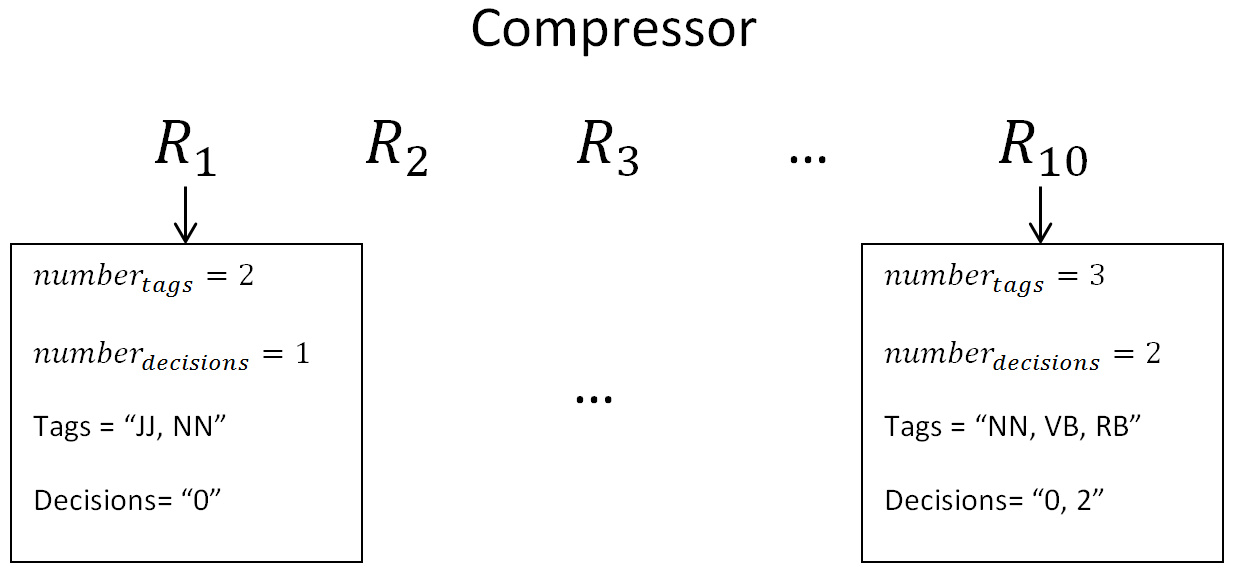
Figure 1: An example of a PARSEC compressor with 10 rules.

In the following explanation, let X denote some original dataset for which PARSEC is being applied to, and let Y denote the equivalent POS dataset. Furthermore, let $X_{i,j}$ denote sentence $i$ and word $j$ in $X$, and $Y_{i,j}$ denote sentence $i$ and word $j$ in $Y$.

The compressor in the figure has 10 rules denoted as $R_{1}$, $R_{2}$, $R_{3}$, …, $R_{10}$. The first rule, $R_{1}$, has 2 tags which are represented by the sequence “JJ, NN”. This rule has one decision, and that is, to delete the word at index 0. This implies that when this particular compressor is applied, rule $R_{1}$ will find POS tags in $Y$ corresponding to the sequence “JJ NN”. Let $Y_{l,m}$ and $Y_{l,m+1}$ denote two consecutive words in $Y$ which have the sequence “JJ NN”. The decision in $R_{1}$ is to delete index 0, thus $R_{1}$ will delete $Y_{l,m}$ and consequently it will delete $X_{l,m}$. Thus, the size of $X$ and $Y$ has been reduced by one. Each time $R_{1}$ finds the exact sequence “JJ NN”, the POS tag and word corresponding to “JJ” (index 0) in $Y$ and $X$ are deleted.

Similarly for $R_{10}$, Let $Y_{l,m}$, $Y_{l,m+1}$ and $Y_{l,m+2}$ denote three consecutive words in $Y$ which have the sequence “NN VB RB”. The decision in $R_{10}$ is to delete index 0 and 2, thus $R_{10}$ will delete $Y_{l,m}$, $Y_{l,m+2}$, $X_{l,m}$ and $X_{l,m+2}$ from $Y$ and $X$ respectively for each occurrence of the POS tags “NN VB RB”.

When a rule is being processed, if a punctuation mark occurs, then the rule evaluation immediately stops. This mechanism was incorporated so that the sequence of tags – which is encapsulated by a rule – is applied to a single sentence and is not applied across two separate sentences. For example, consider the two following sentences “This book was really funny. Great, tomorrow is Friday.” which corresponds to: “DT NN VBD RB JJ. JJ, NN VBZ NNP.” Assume that some rule has the following tags “JJ JJ” and the decision is to delete both indices. If the punctuation marks are not taken into consideration, then the rule will match with the words “funny” and “great”. This will result in “This book was really . , tomorrow is Friday.” Consequently, the sentiments in these two sentences are no longer positive. However, if punctuation is taken into consideration, then the rule will not delete any words since the full stop separates the two sentences.

In this study, we define the term ‘wildcard’, which represents the notion of ‘any POS’ tag and is denoted with a ‘*’ symbol. Thus, when a rule is being evaluated, the wildcard POS can match with any POS in the POS dataset. For example, if a rule has the following tags: “JJ * NNP”, then any POS sequence that has ‘JJ’, followed by any POS, followed by ‘NNP’ will cause the rule to match with that POS sequence.

Algorithm 1 presents the generalized pseudocode to match the tags in a rule with the POS tags in the POS dataset. The algorithm also presents how to delete words from the original and POS dataset once a rule matches with a sequence.

1

2

3

input : compressor the compressor to evaluate

input : original_sentence the original sentence

input : POS_sentence the POS sentence

input : length_sentence the length of the sentence to evaluate

4

5begin

6      

7      for each rule in compressor do

8            

9            tag_in_rule $\leftarrow$ the tags inside rule

10            rule_decisions $\leftarrow$ the decisions inside rule

11            for $i\leftarrow 0$ to length_sentence do

12                  

13                  match $\leftarrow$ true

14                  for $j\leftarrow 0$ to length(tag_in_rule) do

15                        

16                        if tag_in_rule [$j$] not equal POS_sentence [$i+j$] then

17                               match $\leftarrow$ false

18                              break loop and go to line 5

19                        

20                  

21                  if match equal true then

22                        

23                        for $k\leftarrow 0$ to length(rule_decisions) do

24                              

25                              flag original_sentence [$i+\textnormal{{rule\_decisions}}[k]$]

26                        

27                  

28            

29            compressed_sentence $\leftarrow$ delete all words in original_sentence that have been flagged.

30      

31

return compressed_sentence

Algorithm 1 Pseudocode to apply a compressor to a sentence and compress the text.

III-B PARSEC initial population generation

The pseudocode for creating an initial population of compressors is presented in algorithm 2. Several individuals are created based on a predefined user parameter, namely the population size. Several rules have to be created for each compressor. There must be at least one rule, and a user-defined parameter, namely max_rules, is implemented to restrict the total number of rules. When creating the rules, the algorithm iterates until it has reached max_rules, and a probability value of 0.5 was set to determine if a rule was to be created or not, as can be seen on line 9 in algorithm 2. Each rule consists of two primary parts, namely the tags and the decisions, the pseudocode for the creation of those respective parts are presented in algorithms 3 and 4.

1

2

input : population_size the number of compressors to create

3

4begin

5      

6      for $i\leftarrow 0$ to population_size do

7            

8            CreateCompressor()

9            Evaluate compressor.

10            Add compressor to the initial population.

11      

12      Function CreateCompressor ()

13            

14            new_compressor $\leftarrow$ create a blank compressor

15            for $j\leftarrow 0$ to max_tags do

16                  

17                  if rand() $<$ 0.5 then

18                        

19                        CreateRule() and add rule to new_compressor

20                  

21            

22            if Compressor has no rule then

23                  

24                  CreateRule() and add rule to new_compressor

25            

26            return new_compressor

27      

28      Function CreateRule ()

29            

30            new_rule $\leftarrow$ create a blank rule

31            Create the tags using algorithm 3 and add the rules to new_rule.

32            Create the decisions using algorithm 4 and add the rules to new_rule.

33      

34

return The initial population.

Algorithm 2 Pseudocode to create the initial population of compressors.

1

input : minimum_tags the minimum number of allowed pos tags

input : maximum_tags the maximum number of allowed pos tags

2

3begin

4      

5      pos_list $\leftarrow$ { }

6      number_tags $\leftarrow$ random[minimum_tags, maximum_tags ]

7      for $i\leftarrow 0$ to number_tags do

8            

9            if $i$ = 0 then

10                  

11                  Create a tag (excluding wildcard) and add it to pos_list

12            else if $i$ = number_tags-1 then

13                  

14                  Create a tag (excluding wildcard) and add it to pos_list

15            else

16                  

17                  Create a tag (including wildcard) and add it to pos_list

18            

19      

20

return pos_list

Algorithm 3 Pseudocode to create POS tags.

1

input : number_tags the number of tags

2

3begin

4      

5      for $i\leftarrow 0$ to number_tags do

6            

7            if random[0,1] $<$ 0.5 then

8                  

9                  Add $i$ to decision_list

10            

11      

12

return decision_list.

Algorithm 4 Pseudocode to create decisions.

1

2

3

input : sentence the sentence to be evaluated

input : dictionary the dictionary of sentiment words

input : negation_words the list of negation words

output : The sentiment for the evaluated sentence

4

5begin

6      

7      sentiment_score $\leftarrow$ 0

8      negation $\leftarrow$ false

9      for each word in the sentence do

10            

11            if word is in dictionary and negation is true then

12                   sentiment_score $\leftarrow$ sentiment_score + (-1 $\times$ word’s sentiment value)

13            

14            if word is in dictionary and negation is false then

15                  

16                  sentiment_score $\leftarrow$ sentiment_score + word’s sentiment value

17            

18            if word is in negation_words then

19                  

20                  negation $\leftarrow$ swap polarity

21            else

22                   negation $\leftarrow$ false

23            

24      

25      return sentiment_score

26

Algorithm 5 Pseudocode for baseline evaluation.

III-C PARSEC fitness function

The pseudocode for the fitness evaluation of a compressor is presented in algorithm 6. Each instance in the dataset is considered in turn. The sentiment for each instance in the original dataset is computed using algorithm 5. When a compressor is evaluated, it is applied to each instance and a compressed sentence is created. The sentiment of each compressed sentence is computed using algorithm 5. The compressed sentiment is then compared to the original sentiment. If these are the same then the compressed sentence has had no effect on the sentiment when compared to the original. Conversely, if the values are different, then there are two possibilities. Either the compressed sentiment is equal to the correct sentiment as labelled in the training data (in which case the compressor is rewarded) or it is not (in which case the compressor is penalised). Thus, the fitness function takes into consideration the number of new instances for which the compressor produces the correct result.

A multi-objective fitness function was created to combine the fitness, the average reduction in terms of the length of the sentences before and after compression, and the size of the compressor in terms of the number of rules. Thus, the objective was to maximize the fitness and average reduction in sentences, and to minimize the size of the compressor.

1

2

3

input : compressor the compressor to evaluated

input : sentence a list of sentences for which compressor will be evaluated on

input : original_lengths a list of lengths for each sentence in the original data set

input : original_sentiments a list of sententiment values determined by applying algorithm 5 on the original data set

input : correct_sentiments a list of correct sententiment values for the original data set

input : number_rules the number of rules that compressor has

output : The sentiment for the evaluated sentence

4

5begin

6      

7      for $i\leftarrow 1$ to number_of_sentences do

8            

9            compressed_sentence $\leftarrow$ apply compression to sentences [$i$].

10            compressed_sentiment $\leftarrow$ apply algorithm 5.

11            if compressed_sentiment is not equal to original_sentiments [$i$] then

12                  

13                  if compressed_sentiment is equal to correct_sentiments [$i$] then

14                        

15                        raw_fitness $\leftarrow$ raw_fitness + 1

16                  else

17                        

18                        raw_fitness $\leftarrow$ raw_fitness- 1

19                  

20            

21            average_change $\leftarrow$ average_change + (Length(sentences [$i$]) - Length(compressed_sentence))

22      

23      raw_fitness $\leftarrow$ raw_fitness + [0.5 $\times$ (average_change/ number_of_sentences)] - (0.1 $\times$ number_rules)

24

25return raw_fitness

Algorithm 6 Pseudocode to compute fitness of a compressor.

IV Experimental Setup

IV-A Datasets and Setup

Twelve data sets were created by randomly selecting reviews from corresponding Amazon review datasets [12]. For each created data set, 1000 positive and 1000 negative reviews were randomly selected from the larger corresponding Amazon data set. The larger Amazon data sets were obtained from [12, 13]. The data sets were: Amazon Instant Video (AIV), Apps for Android, Automotive, Baby, Beauty, Digital Music, Health and Personal Care, Musical Instruments (MI), Patio Lawn and Garden, Pet Supplies, Tools and Home Improvement, and Toys and Games.

We propose a set of experiments whereby the compression rate is a user parameter and PARSEC must generate compressors that can compress the original datasets to reach the specified compression rate.

To achieve this, a lower and upper user-defined compression bound were defined. The lower compression bound (LCB) was implemented to ensure that the compressors did not result in a compression ratio less than the specified value. Similarly, the upper compression bound (UCB) ensured that the compressors did not result in a compression ratio greater than the specified value. Thus, every compressor in the EA population had to have a compression rate between the LCB and UCB.

Furthermore, two additional user-defined parameters were implemented to ensure that the total number of rules within each compressor remained within a certain bound. The two parameters were named $compressionRules_{min}$ and $compressionRules_{max}$. The $compressionRules_{max}$ parameter prevents compressors from having an extremely large number of rules. Both parameters aid in restricting the search space in terms of the number of rules to create and maintain for each compressor during the evolutionary process. The initial population generation had to respect the LCB and UCB, and respect the minimum and maximum number of rules. The mutation operator also had to respect these constraints.

IV-B Sentiment analysis algorithms

Several sentiment analysis algorithms were applied to the original and compressed datasets to determine the difference in accuracy and to investigate the performance of PARSEC. The following algorithms were used: SentiStrength [14, 15], MeaningCloud [16], Vivek [17], Stanford [18], uClassify [19], Sentiment140 [20], Intellexer [21] and LingPipe [22].

IV-C Execution of experiments

We first applied the sentiment analysis algorithms described in section IV-B to the original datasets and record the test accuracy. Then, we ran PARSEC using the baseline evaluation to create compressor rules. Once the compressors were created, we applied the compressors to the original datasets to generate the compressed data. We applied the sentiment analysis algorithms on the compressed data and recorded the test accuracy. In the following section we report on the change in accuracy between the compressed and original data. PARSEC evolved a population of 250 compressors over 100 generations, the crossover rate was 60% and mutation rate was 40%.

TABLE I: The lower (LCB) and upper (UCB) compression bound constrain the algorithm by ensuring that the compression rate for each compressor is between the two values respectively. The table presents the LCB and UCB values (%) along with the minimum and maximum number of rules used in the experiments. These set compression rates were enforced and the performance of PARSEC was measured on several datasets. The values for the minimum and maximum number of rules were determined by additional trial runs. It was observed that a greater number of rules were needed to achieve higher compression rates.

LCB	UCB	$compression\allowbreak Rules_{min}$	$compression\allowbreak Rules_{max}$
10	13	5	50
15	18	10	70
20	13	20	90
25	28	40	120
30	33	90	150
50	53	350	500

V Results and Conclusion

Figure 2 shows the average change in test accuracy across the different methods based on the compression rates. The general trend is a decrease in performance with the largest decrease in performance observed by Sentiment140. LingPipe and SentiStrength were the only two methods that achieved a positive change in performance (on certain datasets) on compression rates of 10% and 15% respectively. When experimenting with PARSEC we posed the following question. For a predetermined drop in accuracy, how much compression is achievable by PARSEC? For a threshold of -1% compression, Vivek and LingPipe were able to achieve up to 30% compression. For this same threshold five methods could achieve up to 20% compression rate. Regardless of the compression rate used, both Stanford and Sentiment140 did not obtain any result less than -1%. These two algorithms produced the weakest performance with PARSEC.

Figure 2: Change in average test accuracy across the different sentiment analysis algorithms for different text compression rates enforced by PARSEC, averaged across all the data sets. A higher positive value indicates a better result. The various sentiment analysis technologies are denoted as follows: IN, LP, MC, S140, SS, ST, uC and V refer to Intellexer, LingPipe, MeaningCloud, Sentiment140, SentiStrength, Stanford, uClassify and Vivek respectively. The accuracy obtained by LingPipe outperformed all the other methods. Furthermore, LingPipe obtained an average positive change in accuracy of 0.1% for 10% compression. At a compression rate of 50%, LingPipe obtained an change in accuracy of -1.2% averaged over all the datasets, illustrating that it works well with PARSEC.

For a threshold of -2%, five algorithms could achieve up to 30% compression rate and LingPipe was able to achieve up to 50% compression. When the threshold is set to -3% four methods could achieve up to 50% compression.

We additionally wanted to determine the change in test accuracy when a much larger compression rate was used. Table II presents the results when a compression rate of 75% was used. Only certain algorithms were tested due to our limited access to the sentiment analysis algorithms. These results reveal that a large compression rate is achievable without a great loss in test accuracy: LingPipe obtained a loss of -3.3% accuracy.

An example of PARSEC compression is as follows. The original sentence (which contains 56 words and is already stemmed): “this be a wonderful movie involve fascinating people who be such great actor and actress. the event be interesting and I never get tire of watch the episode. I be so sad to see that they be not go to keep go with the life of all these inhabitant of Lark rise and candleford. Mrs. Hamlin”. The compressed sentence (22 words): “this be wonderful movie involve fascinating people who actress. get tire. so sad to see not keep go rise candleford. Mrs. Hamlin”.

TABLE II: Average change in test accuracy (%) across all the data sets when PARSEC models were created for 75% compression rate.

Algorithm	Change in Test Accuracy	Original Accuracy	Compressed Accuracy
LingPipe	-3.2	79.7	76.4
MeaningCloud	-4.2	62.5	58.2
SentiStrength	-6.9	67.8	60.8
uClassify	-6.4	80.7	74.3

Below are four rules which were randomly selected from a PARSEC model to illustrate some of the evolved rules. This model had a total of 38 rules. The POS tags are presented in order of appearance between square brackets. The indices start from zero. Rule 1 denotes that if the POS “NNP” is followed by “JJ”, then delete both words. Rule 4 denotes that if “IN” is followed by any POS and then followed by “VB”, then delete the word at index 1.

• Rule 1: [NNP, JJ]. Number of decisions: 2.
  Decisions: [0, 1]

• Rule 2: [VBG, NNP]. Number of decisions: 2.
  Decisions: [0, 1]

• Rule 3: [IN, CC]. Number of decisions: 2.
  Decisions: [0, 1]

• Rule 4: [IN, *, VB]. Number of decisions: 1.
  Decisions: [1]

This study empirically demonstrates that machine learning can reduce the amount of data needed to determine the sentiments within sentences with little loss in accuracy. To achieve this, we proposed an evolutionary algorithm, PARSEC, which evolves a population of chromosomes which encode rules for compression based on the removal of POS.

We studied the test accuracies achieved by the eight algorithms when set compression rate thresholds were enforced. Two algorithms showed marginal improvements in accuracy on several data sets for a compression rate of 15%. Additionally, there were 9 data sets whereby some of the algorithms were able to yield an improvement in accuracy for a compression rate of 30%. At a threshold of -1% sentiment accuracy loss, two methods were able to achieve up to 30% compression, five methods up to 20% compression, and six methods up to 10% compression. The best performing algorithm, LingPipe, showed only modest losses in accuracy even at high compression: 3.3% for a four-fold data compression.

It would be of interest to incorporate the PARSEC algorithm directly into a sentiment analysis algorithm instead of via a simple dictionary approach. One could achieve this by replacing the fitness function used in the evolutionary phase with a more sophisticated sentiment analysis algorithm. This would allow the emergence of an algorithm where the compression and sentiment analysis are mutually optimised for best performance.

Appendix A Detailed results for fixed compression rate experiments

Tables III to VIII present the difference in test accuracy results for the various compression rates. The various sentiment analysis algorithms are abbreviated as follows: IN, LP, MC, S140, SS, ST, uC and V refer to Intellexer, LingPipe, MeainingCloud, Sentiment140, SentiStrength, Stanford, uClassify and Vivek respectively. For a compression rate of 10%, the best and worst change in accuracy were obtained by LingPipe and Sentiment140 respectively. Based on all the findings for 10 per cent compression, there were 21 cases across all the methods and data sets whereby the change in accuracy was greater than zero. For a compression rate of 15% the number of cases was 17 whereby LingPipe obtained the best average change in accuracy with a value of 0.0%.

The best change in accuracy for 20% compression rate was obtained by uClassify with a value of 0.7 on two data sets. There were six data sets for which uClassify reduced the data up to 20% and for which the test accuracy on the compressed data was better than on the original data. Additionally, there were 14 cases in total across all the algorithms whereby the change in accuracy was greater than zero for 20% compression.

The findings revealed that a for the compression rate of 25% there were 14 cases for which the change was greater than zero, and the best change in average accuracy was obtained once again by LingPipe with a value of -0.3%. There was a reduction performance in terms of the number of cases having a change greater than zero when a compression of 30% was used; notably 9 cases. uClassify however, on 5 datasets, had a test accuracy greater than zero. Finally, only two algorithms were able to obtain improvements in terms of the changes for a compression rate of 50%, namely uClassify and LingPipe, with changes in 3 and 2 data sets respectively.

	IN	LP	MC	S140	SS	ST	uC	V
AIV	-0.9	-0.0	0.4	-2.1	-0.3	-3.0	-1.9	-0.9
MI	0.1	0.3	-0.7	-1.9	-0.4	0.5	-0.4	-1.4
Digital Music	-1.0	0.2	-0.3	-2.5	-0.1	-1.9	-0.4	-2.0
Baby	0.0	0.4	-0.2	-2.7	0.0	-1.2	0.3	0.2
Patio & Garden	-0.1	0.4	-0.2	-2.1	-0.2	-0.7	0.9	-0.9
Automotive	-1.1	0.4	-0.5	-2.1	0.0	-1.1	0.7	-0.9
Pet Supplies	-1.2	0.3	-0.4	-2.9	-0.4	0.3	0.0	-1.6
Apps for Android	-1.4	0.0	-0.5	-2.5	-0.3	-3.5	0.0	-1.6
Beauty	-0.5	0.0	0.2	-1.2	0.0	-0.5	-0.7	-0.4
Tools & Home	0.8	-0.1	-1.0	-2.3	-0.6	-1.7	0.5	0.0
Toys & Games	-0.5	0.0	-1.5	-1.8	0.2	-3.1	-0.1	-1.4
Health & Personal	0.4	0.1	-0.4	-1.6	-0.3	-1.4	0.5	-0.4
Average	-0.4	0.1	-0.4	-2.1	-0.2	-1.4	0.0	-0.9

TABLE III: Difference between the compressed and original test accuracy when a compression rate between 10% and 13% was imposed.

	IN	LP	MC	S140	SS	ST	uC	V
AIV	-1.1	-1.1	-0.2	-2.7	0.1	-3.2	-2.0	-0.6
MI	1.1	0.5	-0.8	-2.9	-0.8	0.0	-1.3	-0.8
Digital Music	-1.6	0.4	-0.7	-3.6	-0.5	-2.3	-1.2	-2.1
Baby	0.0	-0.9	-0.5	-2.4	0.2	-2.0	0.6	-0.1
Patio & Garden	-0.3	-0.4	-0.3	-3.5	-0.6	-1.2	0.5	-1.0
Automotive	-1.4	0.6	-1.0	-2.8	-0.3	-2.2	0.9	-0.8
Pet Supplies	-1.1	0.6	-0.2	-3.8	-0.6	-1.3	0.2	-2.9
Apps for Android	-1.7	-0.3	-0.9	-4.2	-0.5	-3.4	-1.0	-3.2
Beauty	-0.9	-0.3	-0.7	-3.5	-0.2	-1.3	-1.8	-1.2
Tools & Home	-0.2	0.0	0.0	-3.0	-0.3	-1.7	1.2	0.7
Toys & Games	-1.3	-0.2	-1.2	-1.6	-0.1	-1.1	-0.8	-1.8
Health & Personal	0.1	0.0	-0.6	-2.8	-0.5	-2.6	0.2	-0.4
Average	-0.7	0.0	-0.6	-3.0	-0.3	-1.8	-0.3	-1.2

TABLE IV: Difference between the compressed and original test accuracy when a compression rate between 15% and 18% was imposed.

	IN	LP	MC	S140	SS	ST	uC	V
AIV	-1.7	-1.2	0.3	-4.0	-0.4	-3.1	-1.8	-1.8
MI	0.2	1.1	-1.1	-2.5	-0.6	0.4	-1.2	-1.4
Digital Music	-2.2	-0.4	-0.2	-3.5	-1.2	-3.1	-1.7	-2.0
Baby	-0.7	-0.4	-0.4	-2.7	-0.8	-2.2	0.5	-1.1
Patio & Garden	-0.9	-1.1	-1.2	-3.7	-0.5	-2.2	0.5	-0.9
Automotive	-1.6	0.2	-0.3	-3.5	-0.9	-2.8	0.3	-1.7
Pet Supplies	-1.0	0.4	-1.3	-3.5	-0.4	-2.1	0.7	-2.2
Apps for Android	-1.7	-0.1	-1.6	-4.8	-0.4	-4.5	-1.7	-3.3
Beauty	-1.1	0.2	-0.6	-4.0	-1.0	-1.1	-1.2	-1.2
Tools & Home	0.6	-0.1	-1.2	-4.4	-0.7	-1.9	0.0	-1.5
Toys & Games	-1.5	0.0	-0.4	-3.3	-0.2	-2.8	-1.5	-1.9
Health & Personal	0.0	-0.4	-1.0	-4.2	-1.2	-1.7	0.7	-0.9
Average	-0.9	-0.1	-0.7	-3.7	-0.7	-2.2	-0.5	-1.6

TABLE V: Difference between the compressed and original test accuracy when a compression rate between 20% and 23% was imposed.

	IN	LP	MC	S140	SS	ST	uC	V
AIV	-2.4	-1.6	-0.6	-3.7	-0.2	-6.0	-2.5	-2.0
MI	-0.6	1.0	-0.1	-4.8	-1.0	-1.6	-0.1	-1.8
Digital Music	-1.9	-0.1	-0.5	25.1	-0.5	-2.4	-2.9	-3.5
Baby	0.1	-0.9	0.5	-4.4	-0.5	-2.6	-0.4	-0.6
Patio & Garden	-0.9	-1.4	0.1	-4.7	-0.9	-1.5	0.6	-1.6
Automotive	-2.0	0.1	0.1	-3.3	-1.5	-4.2	0.5	-0.4
Pet Supplies	-0.8	0.0	-0.7	-5.3	-0.6	-1.7	0.1	-2.9
Apps for Android	-2.4	-0.4	-1.4	-6.7	-0.9	-3.4	-0.9	-3.4
Beauty	-1.1	0.2	-0.7	-5.5	-0.6	-2.1	-1.8	-2.4
Tools & Home	-0.8	-1.0	-1.6	-5.2	-1.1	-3.6	0.0	-0.3
Toys & Games	-1.2	-0.5	-1.1	-5.7	-0.2	-2.7	-1.0	-3.6
Health & Personal	0.3	0.9	0.0	-3.9	-0.3	-2.8	-0.9	-1.1
Average	-1.1	-0.3	-0.5	-2.3	-0.7	-2.9	-0.7	-1.9

TABLE VI: Difference between the compressed and original test accuracy when a compression rate between 25% and 28% was imposed.

	IN	LP	MC	S140	SS	ST	uC	V
AIV	-2.3	-2.1	-0.1	-8.2	-1.3	-7.0	-2.3	-2.5
MI	-0.5	0.6	-1.1	-6.9	-1.6	-2.4	-1.9	-2.8
Digital Music	-3.3	-1.1	-1.0	-6.2	-1.7	-3.6	-2.8	-4.9
Baby	-0.8	-0.7	0.2	-6.1	-1.1	-5.3	0.7	-1.3
Patio & Garden	-1.8	-1.2	-1.7	-6.6	-1.5	-4.3	-0.3	-2.2
Automotive	-1.2	-0.4	-0.9	-4.8	-1.5	-4.7	0.8	-2.6
Pet Supplies	-2.2	-0.9	-1.1	-5.8	-1.0	-4.4	1.6	-2.8
Apps for Android	-3.0	0.0	-2.1	-7.7	-1.1	-6.4	-2.1	-5.3
Beauty	-2.4	-0.2	-1.1	-7.7	-1.2	-4.6	-1.9	-3.2
Tools & Home	-0.9	0.0	-1.3	-5.9	-1.5	-5.0	0.4	-1.1
Toys & Games	-2.2	0.0	-1.6	-6.0	-0.2	-5.0	-0.7	-3.0
Health & Personal	-0.6	-0.3	-0.60	-6.10	-0.70	-5.30	0.70	-2.00
Average	-1.8	-0.5	-1.0	-6.5	-1.2	-4.8	-0.6	-2.8

TABLE VII: Difference between the compressed and original test accuracy when a compression rate between 30% and 33% was imposed.

	IN	LP	MC	S140	SS	ST	uC	V
AIV	-5.8	-4.2	-1.8	-15.6	-3.4	-13.2	-7.8	-8.2
MI	-1.9	0.8	-0.9	-15.1	-2.6	-6.9	-3.9	-7.6
Digital Music	-5.5	-1.3	-1.9	-15.3	-3.5	-9.9	-5.5	-9.0
Baby	-1.4	-1.4	-1.7	-12.4	-2.4	-11.2	-1.5	-5.6
Patio & Garden	-3.8	-1.8	-2.1	-13.9	-2.5	-10.1	-0.5	-4.7
Automotive	-3.7	-2.4	-1.9	-12.6	-2.8	-7.9	0.1	-4.6
Pet Supplies	-1.8	-1.6	-2.2	-14.9	-2.5	-8.0	0.6	-6.2
Apps for Android	-6.2	-1.6	-4.8	-17.1	-4.4	-12.4	-4.3	-11.0
Beauty	-3.0	-0.1	-1.8	-15.3	-3.0	-8.7	-4.1	-7.8
Tools & Home	-2.2	0.1	-2.2	-14.3	-3.6	-9.5	1.0	-4.9
Toys & Games	-4.8	-1.2	-2.0	-12.7	-1.8	-10.1	-4.3	-7.2
Health & Personal	-2.2	-0.2	-2.0	-12.1	-2.2	-10.1	-1.1	-5.0
Average	-3.5	-1.2	-2.1	-14.3	-2.9	-9.8	-2.6	-6.8

TABLE VIII: Difference between the compressed and original test accuracy when a compression rate between 50% and 53% was imposed.

References

- [1] B. Pang and L. Lee, “Opinion mining and sentiment analysis,” Found. Trends Inf. Retr., vol. 2, no. 1-2, pp. 1–135, Jan. 2008.
- [2] B. Liu, Sentiment Analysis: Mining Opinions, Sentiments, and Emotions. Cambridge University Press, 2015.
- [3] K. Ravi and V. Ravi, “A survey on opinion mining and sentiment analysis,” Know.-Based Syst., vol. 89, no. C, pp. 14–46, Nov. 2015.
- [4] A. E. Eiben and J. E. Smith, Introduction to Evolutionary Computing. SpringerVerlag, 2003.
- [5] X. Yu and M. Gen, Introduction to Evolutionary Algorithms. Springer Publishing Company, Incorporated, 2012.
- [6] S. Feng, D. Wang, G. Yu, B. Li, and K.-F. Wong, A Chinese Sentence Compression Method for Opinion Mining. Berlin, Heidelberg: Springer Berlin Heidelberg, 2010, pp. 320–329.
- [7] W. Che, Y. Zhao, H. Guo, Z. Su, and T. Liu, “Sentence compression for aspect-based sentiment analysis,” IEEE/ACM Trans. Audio, Speech and Lang. Proc., vol. 23, no. 12, pp. 2111–2124, Dec. 2015.
- [8] T. Mikolov, K. Chen, G. Corrado, and J. Dean, “Efficient estimation of word representations in vector space,” arXiv preprint arXiv:1301.3781, 2013.
- [9] K. Toutanova, D. Klein, C. D. Manning, and Y. Singer, “Feature-rich part-of-speech tagging with a cyclic dependency network,” in Proceedings of the 2003 Conference of the North American Chapter of the Association for Computational Linguistics on Human Language Technology - Volume 1, ser. NAACL ’03. Stroudsburg, PA, USA: Association for Computational Linguistics, 2003, pp. 173–180.
- [10] M. P. Marcus, M. A. Marcinkiewicz, and B. Santorini, “Building a large annotated corpus of english: The penn treebank,” Comput. Linguist., vol. 19, no. 2, pp. 313–330, Jun. 1993.
- [11] A. Taylor, M. Marcus, and B. Santorini, Treebanks: Building and Using Parsed Corpora. Dordrecht: Springer Netherlands, 2003, ch. The Penn Treebank: An Overview, pp. 5–22.
- [12] J. Leskovec and A. Krevl, “SNAP Datasets: Stanford large network dataset collection,” http://snap.stanford.edu/data, Jun. 2014.
- [13] J. McAuley, R. Pandey, and J. Leskovec, “Inferring networks of substitutable and complementary products,” in Proceedings of the 21th ACM SIGKDD International Conference on Knowledge Discovery and Data Mining, ser. KDD ’15. New York, NY, USA: ACM, 2015, pp. 785–794.
- [14] M. Thelwall, K. Buckley, G. Paltoglou, D. Cai, and A. Kappas, “Sentiment in short strength detection informal text,” J. Am. Soc. Inf. Sci. Technol., vol. 61, no. 12, pp. 2544–2558, Dec. 2010.
- [15] M. Thelwall, K. Buckley, and G. Paltoglou, “Sentiment strength detection for the social web,” J. Am. Soc. Inf. Sci. Technol., vol. 63, no. 1, pp. 163–173, Jan. 2012.
- [16] MeaningCloud, “Meaningcloud is a brand by meaningcloud llc, a s—ngular company.” https://www.meaningcloud.com/, 2015.
- [17] V. Narayanan, I. Arora, and A. Bhatia, “Fast and accurate sentiment classification using an enhanced naive bayes model,” in Proceedings of the 14th International Conference on Intelligent Data Engineering and Automated Learning — IDEAL 2013 - Volume 8206, ser. IDEAL 2013. New York, NY, USA: Springer-Verlag New York, Inc., 2013, pp. 194–201.
- [18] R. Socher, A. Perelygin, J. Y. Wu, J. Chuang, C. D. Manning, A. Y. Ng, and C. Potts, “Recursive deep models for semantic compositionality over a sentiment treebank,” in Proceedings of the conference on empirical methods in natural language processing (EMNLP), 2013, pp. 1631–1642.
- [19] uClassify, “uclassify,” https://www.uclassify.com/, 2008.
- [20] A. Go, R. Bhayani, and L. Huang, “Twitter sentiment classification using distant supervision,” Technical report, Stanford, 2009.
- [21] EffectiveSoft, “Intellexer,” http://www.intellexer.com/, 2000.
- [22] Alias-i., “Lingpipe 4.1.0,” http://alias-i.com/lingpipe, 2008.