Minimum Covariance Determinant and Extensions

Abstract

The Minimum Covariance Determinant (MCD) method is a highly robust estimator of multivariate location and scatter, for which a fast algorithm is available. Since estimating the covariance matrix is the cornerstone of many multivariate statistical methods, the MCD is an important building block when developing robust multivariate techniques. It also serves as a convenient and efficient tool for outlier detection.

The MCD estimator is reviewed, along with its main properties such as affine equivariance, breakdown value, and influence function. We discuss its computation, and list applications and extensions of the MCD in applied and methodological multivariate statistics. Two recent extensions of the MCD are described. The first one is a fast deterministic algorithm which inherits the robustness of the MCD while being almost affine equivariant. The second is tailored to high-dimensional data, possibly with more dimensions than cases, and incorporates regularization to prevent singular matrices.

INTRODUCTION

The Minimum Covariance Determinant (MCD) estimator is one of the first affine equivariant and highly robust estimators of multivariate location and scatter ^{1, 2}. Being resistant to outlying observations makes the MCD very useful for outlier detection. Although already introduced in 1984, its main use has only started since the construction of the computationally efficient FastMCD algorithm of ³ in 1999. Since then, the MCD has been applied in numerous fields such as medicine, finance, image analysis and chemistry. Moreover the MCD has also been used to develop many robust multivariate techniques, among which robust principal component analysis, factor analysis and multiple regression. Recent modifications of the MCD include a deterministic algorithm and a regularized version for high-dimensional data.

DESCRIPTION OF THE MCD ESTIMATOR

Motivation

In the multivariate location and scatter setting the data are stored in an $n\times p$ data matrix ${\bm{X}}=({\bm{x}}_{1},\ldots,{\bm{x}}_{n})^{\prime}$ with ${\bm{x}}_{i}=(x_{i1},\ldots,x_{ip})^{\prime}$ the $i$-th observation, so $n$ stands for the number of objects and $p$ for the number of variables. We assume that the observations are sampled from an elliptically symmetric unimodal distribution with unknown parameters $\bm{\mu}$ and $\bm{\Sigma}$, where $\bm{\mu}$ is a vector with $p$ components and $\bm{\Sigma}$ is a positive definite $p\times p$ matrix. To be precise, a multivariate distribution is called elliptically symmetric and unimodal if there exists a strictly decreasing real function $g$ such that the density can be written in the form

$$f({\bm{x}})=\frac{1}{\sqrt{|\bm{\Sigma}|}}\;g(d^{2}({\bm{x}},\bm{\mu},\bm{\Sigma}))$$ (1)

in which the statistical distance $d({\bm{x}},\bm{\mu},\bm{\Sigma})$ is given by

$$d({\bm{x}},\bm{\mu},\bm{\Sigma})=\sqrt{({\bm{x}}-\bm{\mu})^{\prime}\bm{\Sigma}^{-1}({\bm{x}}-\bm{\mu})}\ \ .$$ (2)

To illustrate the MCD, we first consider the wine data set available in ⁴ and also analyzed in ⁵. This data set contains the quantities of 13 constituents found in three types of Italian wines. We consider the first group containing 59 wines, and focus on the constituents ‘Malic acid’ and ‘Proline’. This yields a bivariate data set, i.e. $p=2$. A scatter plot of the data is shown in Figure 1, in which we see that the points on the lower right hand side of the plot are outlying relative to the majority of the data.

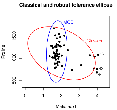
Figure 1: Bivariate wine data: tolerance ellipse of the classical mean and covariance matrix (red), and that of the robust location and scatter matrix (blue).

In the figure we see two ellipses. The classical tolerance ellipse is defined as the set of $p$-dimensional points ${\bm{x}}$ whose Mahalanobis distance

$$\text{MD}({\bm{x}})=d({\bm{x}},\bar{{\bm{x}}},\mbox{Cov}(X))=\sqrt{({\bm{x}}-\bar{{\bm{x}}})^{\prime}\mbox{Cov}(X)^{-1}({\bm{x}}-\bar{{\bm{x}}})}$$ (3)

equals $\sqrt{\chi^{2}_{p,0.975}}$. Here $\bar{{\bm{x}}}$ is the sample mean and $\mbox{Cov}(X)$ the sample covariance matrix. The Mahalanobis distance $\text{MD}(\bm{x}_{i})$ should tell us how far away $\bm{x}_{i}$ is from the center of the data cloud, relative to its size and shape. In Figure 1 we see that the red tolerance ellipse tries to encompass all observations. Therefore none of the Mahalanobis distances is exceptionally large, as we can see in Figure 2(a). Based on Figure 2(a) alone we would say there are only three mild outliers in the data (we ignore borderline cases).

On the other hand, the robust tolerance ellipse is based on the robust distances

$$\text{RD}({\bm{x}})=d({\bm{x}},\hat{\bm{\mu}}_{MCD},\hat{\bm{\Sigma}}_{MCD})$$ (4)

where $\hat{\bm{\mu}}_{MCD}$ is the MCD estimate of location and $\hat{\bm{\Sigma}}_{MCD}$ is the MCD covariance estimate, which we will explain soon. In Figure 1 we see that the robust ellipse (in blue) is much smaller and only encloses the regular data points. The robust distances shown in Figure 2(b) now clearly expose 8 outliers.

(a)	(b)

Figure 2: (a) Mahalanobis distances and (b) robust distances for the bivariate wine data.

This illustrates the masking effect: the classical estimates can be so strongly affected by contamination that diagnostic tools such as the Mahalanobis distances become unable to detect the outliers. To avoid masking we instead need reliable estimators that can resist outliers when they occur. The MCD is such a robust estimator.

Definition

The raw Minimum Covariance Determinant (MCD) estimator with tuning constant $n/2\leqslant h\leqslant n$ is $(\hat{\bm{\mu}}_{0},\hat{\bm{\Sigma}}_{0})$ where

1. the location estimate $\hat{\bm{\mu}}_{0}$ is the mean of the $h$ observations for which the determinant of the sample covariance matrix is as small as possible;

2. the scatter matrix estimate $\hat{\bm{\Sigma}}_{0}$ is the corresponding covariance matrix multiplied by a consistency factor $c_{0}$.

Note that the MCD estimator can only be computed when $h>p$, otherwise the covariance matrix of any $h$-subset has determinant zero, so we need at least $n>2p$. To avoid excessive noise it is however recommended that $n>5p$, so that we have at least 5 observations per dimension. (When this condition is not satisfied one can instead use the MRCD method (11) described near the end of this article.) To obtain consistency at the normal distribution, the consistency factor $c_{0}$ equals $\alpha/F_{\chi^{2}_{p+2}}(q_{\alpha})$ with $\alpha=\lim_{n\to\infty}h(n)/n$, and $q_{\alpha}$ the $\alpha$-quantile of the $\chi^{2}_{p}$ distribution ⁶. Also a finite-sample correction factor can be incorporated ⁷.

Consistency of the raw MCD estimator of location and scatter at elliptical models, as well as asymptotic normality of the MCD location estimator has been proved in ⁸. Consistency and asymptotic normality of the MCD covariance matrix at a broader class of distributions is derived in ^{9, 10}.

The MCD estimator is the most robust when taking $h=[(n+p+1)/2]$ where $[a]$ is the largest integer $\leqslant a$. At the population level this corresponds to $\alpha=0.5$. But unfortunately the MCD then suffers from low efficiency at the normal model. For example, if $\alpha=0.5$ the asymptotic relative efficiency of the diagonal elements of the MCD scatter matrix relative to the sample covariance matrix is only 6% when $p=2$, and 20.5% when $p=10$. This efficiency can be increased by considering a higher $\alpha$ such as $\alpha=0.75$. This yields relative efficiencies of 26.2% for $p=2$ and 45.9% for $p=10$ (see ⁶). On the other hand this choice of $\alpha$ diminishes the robustness to possible outliers.

In order to increase the efficiency while retaining high robustness one can apply a weighting step ^{11, 12}. For the MCD this yields the estimates

$$\begin{split}\hat{\bm{\mu}}_{MCD}&=\frac{\sum_{i=1}^{n}W(d_{i}^{2}){\bm{x}}_{i}}{\sum_{i=1}^{n}W(d^{2}_{i})}\\ \hat{\bm{\Sigma}}_{MCD}&=c_{1}\frac{1}{n}\sum_{i=1}^{n}W(d_{i}^{2})({\bm{x}}_{i}-\hat{\bm{\mu}}_{MCD})({\bm{x}}_{i}-\hat{\bm{\mu}}_{MCD})^{\prime}\end{split}$$ (5)

with $d_{i}=d({\bm{x}},\hat{\bm{\mu}}_{0},\hat{\bm{\Sigma}}_{0})$ and $W$ an appropriate weight function. The constant $c_{1}$ is again a consistency factor. A simple yet effective choice for $W$ is to set it to 1 when the robust distance is below the cutoff $\sqrt{\chi^{2}_{p,0.975}}$ and to zero otherwise, that is, $W(d^{2})=I(d^{2}\leqslant\chi^{2}_{p,0.975})$. This is the default choice in the current implementations in R, SAS, Matlab and S-PLUS. If we take $\alpha=0.5$ this weighting step increases the efficiency to 45.5% for $p=2$ and to 82% for $p=10$. In the example of the wine data (Figure 1) we applied the weighted MCD estimator with $\alpha=0.75$, but the results were similar for smaller values of $\alpha$.

Note that one can construct a robust correlation matrix from the MCD scatter matrix. The robust correlation between variables $X_{i}$ and $X_{j}$ is given by

$$r_{ij}=\frac{s_{ij}}{\sqrt{s_{ii}s_{jj}}}$$

with $s_{ij}$ the $(i,j)$-th element of the MCD scatter matrix. In Figure 1 the MCD-based robust correlation is $0.10\approx 0$ because the majority of the data do not show a trend, whereas the classical correlation of $-0.37$ was caused by the outliers in the lower right part of the plot.

Outlier detection

As already illustrated in Figure 2, the robust MCD estimator is very useful to detect outliers in multivariate data. As the robust distances (4) are not sensitive to the masking effect, they can be used to flag the outliers ^{13, 14}. This is crucial for data sets in more than three dimensions, which are difficult to visualize.

We illustrate the outlier detection potential of the MCD on the full wine data set, with all $p=13$ variables. The distance-distance plot of ³ in Figure 3 shows the robust distances based on the MCD versus the classical distances (3). From the robust analysis we see that seven observations clearly stand out (plus some mild outliers), whereas the classical analysis does not flag any of them.

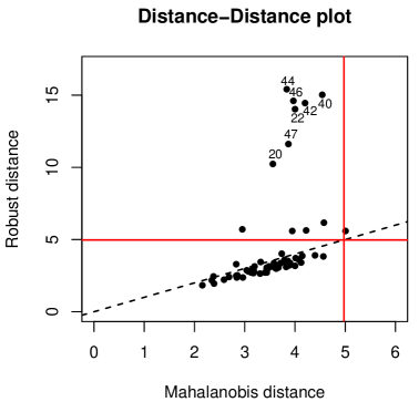
Figure 3: Distance-distance plot of the full 13-dimensional wine data set.

Note that the cutoff value $\sqrt{\chi^{2}_{p,0.975}}$ is based on the asymptotic distribution of the robust distances, and often flags too many observations as outlying. For relatively small $n$ the true distribution of the robust distances can be better approximated by an $F$-distribution, see ¹⁵.

PROPERTIES

Affine equivariance

The MCD estimator of location and scatter is affine equivariant. This means that for any nonsingular $p\times p$ matrix ${\bm{A}}$ and any $p$-dimensional column vector ${\bm{b}}$ it holds that

$$\hat{\bm{\mu}}_{MCD}({\bm{X}}{\bm{A}}^{\prime}+\mathbf{1}_{n}{\bm{b}}^{\prime}) =\hat{\bm{\mu}}_{MCD}({\bm{X}}){\bm{A}}^{\prime}+{\bm{b}}$$ (6)

$$\hat{\bm{\Sigma}}_{MCD}({\bm{X}}{\bm{A}}^{\prime}+\mathbf{1}_{n}{\bm{b}}^{\prime}) ={\bm{A}}\hat{\bm{\Sigma}}_{MCD}({\bm{X}}){\bm{A}}^{\prime}$$ (7)

where the vector $\mathbf{1}_{n}$ is $(1,1,\dots,1)^{\prime}$ with $n$ elements. This property follows from the fact that for each subset $H$ of $\{1,2,\ldots,n\}$ of size $h\,$ and corresponding data set ${\bm{X}}_{H}\,$, the determinant of the covariance matrix of the transformed data equals

$$|{\bm{S}}({\bm{X}}_{H}{\bm{A}}^{\prime})|=|{\bm{A}}{\bm{S}}({\bm{X}}_{H}){\bm{A}}^{\prime}|=|{\bm{A}}|^{2}|{\bm{S}}({\bm{X}}_{H})|.$$

Therefore, transforming an $h$-subset with lowest determinant yields an $h$-subset ${\bm{X}}_{H}{\bm{A}}^{\prime}$ with lowest determinant among all $h$-subsets of the transformed data set ${\bm{X}}{\bm{A}}^{\prime}\,$, and its covariance matrix is transformed appropriately. The affine equivariance of the raw MCD location estimator follows from the equivariance of the sample mean. Finally we note that the robust distances $d_{i}=d({\bm{x}},\hat{\bm{\mu}}_{0},\hat{\bm{\Sigma}}_{0})$ are affine invariant, meaning they stay the same after transforming the data, which implies that the weighted estimator is affine equivariant too.

Affine equivariance implies that the estimator transforms well under any non-singular reparametrization of the space in which the ${\bm{x}}_{i}$ live. Consequently, the data might be rotated, translated or rescaled (for example through a change of measurement units) without affecting the outlier detection diagnostics.

The MCD is one of the first high-breakdown affine equivariant estimators of location and scatter, and was only preceded by the Stahel-Donoho estimator ^{16, 17}. Together with the MCD also the Minimum Volume Ellipsoid estimator was introduced ^{1, 2} which is equally robust but not asymptotically normal, and is harder to compute than the MCD.

Breakdown value

The breakdown value of an estimator is the smallest fraction of observations that need to be replaced (by arbitrary values) to make the estimate useless. For a multivariate location estimator $T_{n}$ the breakdown value is defined as

$$\varepsilon^{*}_{n}(T_{n};{\bm{X}}_{n})=\frac{1}{n}\min\left\{m:\sup||T_{n}({\bm{X}}_{n,m})-T_{n}({\bm{X}}_{n})||=+\infty\right\}$$

where $1\leqslant m\leqslant n$ and the supremum is over all data sets ${\bm{X}}_{n,m}$ obtained by replacing any $m$ data points ${\bm{x}}_{i_{1}},\ldots,{\bm{x}}_{i_{m}}$ of ${\bm{X}}_{n}$ by arbitrary points.

For a multivariate scatter estimator $C_{n}$ we set

$$\varepsilon^{*}_{n}(C_{n};{\bm{X}}_{n})=\frac{1}{n}\min\{m:\sup\;\max_{i}|\log(\lambda_{i}(C_{n}({\bm{X}}_{n,m})))-\log(\lambda_{i}(C_{n}({\bm{X}}_{n})))|=+\infty\}$$

with $\lambda_{1}(C_{n})\geqslant\ldots\geqslant\lambda_{p}(C_{n})>0$ the eigenvalues of $C_{n}\,$. This means that we consider a scatter estimator to be broken when $\lambda_{1}$ can become arbitrarily large (‘explosion’) and/or $\lambda_{p}$ can become arbitrary close to $0$ (‘implosion’). Implosion is a problem because it makes the scatter matrix singular whereas in many situations its inverse is required, e.g. in (4).

Let $k({\bm{X}}_{n})$ denote the highest number of observations in the data set that lie on an affine hyperplane in $p$-dimensional space, and assume $k({\bm{X}}_{n})<h$. Then the raw MCD estimator of location and scatter satisfies ¹⁸

$$\varepsilon^{*}_{n}(\hat{\bm{\mu}}_{0};{\bm{X}}_{n})=\varepsilon^{*}_{n}(\hat{\bm{\Sigma}}_{0};{\bm{X}}_{n})=\frac{\min(n-h+1,h-k({\bm{X}}_{n}))}{n}\;\;.$$ (8)

If the data are sampled from a continuous distribution, then almost surely $k({\bm{X}}_{n})=p$ which is called general position. Then $\varepsilon^{*}_{n}(\hat{\bm{\mu}}_{0};{\bm{X}}_{n})=\varepsilon^{*}_{n}(\hat{\bm{\Sigma}}_{0};{\bm{X}}_{n})=\min(n-h+1,h-p)/n$, and consequently any $[(n+p)/2]\leqslant h\leqslant[(n+p+1)/2]$ gives the breakdown value $[(n-p+1)/2]$. This is the highest possible breakdown value for affine equivariant scatter estimators ¹⁹ at data sets in general position. Also for affine equivariant location estimators the upper bound on the breakdown value is $[(n-p+1)/2]$ under natural regularity conditions ²⁰. Note that in the limit $\lim_{n\to\infty}\varepsilon^{*}_{n}=\min(1-\alpha,\alpha)$ which is maximal for $\alpha=0.5$.

Finally we note that the breakdown value of the weighted MCD estimators $\hat{\bm{\mu}}_{MCD}$ and $\hat{\bm{\Sigma}}_{MCD}$ is not lower than the breakdown value of the raw MCD estimator, as long as the weight function $W$ used in (5) is bounded and becomes zero for large $d_{i}\,$, see ¹¹.

Influence function

The influence function ²¹ of an estimator measures the effect of a small (infinitesimal) fraction of outliers placed at a given point. It is defined at the population level hence it requires the functional form of the estimator $T$, which maps a distribution $F$ to a value $T(F)$ in the parameter space. For multivariate location this parameter space is ${I\hskip-3.0ptR}^{p}$, whereas for multivariate scatter the parameter space is the set of all positive semidefinite $p\times p$ matrices. The influence function of the estimator $T$ at the distribution $F$ in a point ${\bm{x}}$ is then defined as

$$IF({\bm{x}},T,F)=\lim_{\varepsilon\to 0}\frac{T(F_{\varepsilon})-T(F)}{\varepsilon}$$ (9)

with $F_{\varepsilon}=(1-\varepsilon)F+\varepsilon\Delta_{x}$ a contaminated distribution with point mass in ${\bm{x}}$.

The influence function of the raw and the weighted MCD has been computed in ^{6, 10} and turns out to be bounded. This is a desirable property for robust estimators, as it limits the effect of a small fraction of outliers on the estimate. At the standard multivariate normal distribution, the influence function of the MCD location estimator becomes zero for all ${\bm{x}}$ with $\|{\bm{x}}\|^{2}>\chi^{2}_{p,\alpha}$ hence far outliers do not influence the estimates at all. The same happens with the off-diagonal elements of the MCD scatter estimator. On the other hand, the influence function of the diagonal elements remains constant (different from zero) when $\|{\bm{x}}\|^{2}$ is sufficiently large. Therefore the outliers still have a bounded influence on the estimator. All these influence functions are smooth, except at those ${\bm{x}}$ with $\|{\bm{x}}\|^{2}=\chi^{2}_{p,\alpha}\,$. The weighted MCD estimator has an additional jump in $\|{\bm{x}}\|^{2}=\chi^{2}_{p,0.975}$ due to the discontinuity of the weight function, but one could use a smooth weight function instead.

Univariate MCD

For univariate data $x_{1},\ldots,x_{n}$ the MCD estimates reduce to the mean and the standard deviation of the $h$-subset with smallest variance. They can be computed in O($n\log n$) time by sorting the observations and only considering contiguous $h$-subsets so that their means and variances can be calculated recursively ²². Their consistency and asymptotic normality is proved in ^{23, 2}. For $h=[n/2]+1$ the MCD location estimator has breakdown value $[(n+1)/2]/n$ and the MCD scale estimator has $[n/2]/n$. These are the highest breakdown values that can be attained by univariate affine equivariant estimators ²⁴. The univariate MCD estimators also have bounded influence functions, see ⁶ for details. Their maximal asymptotic bias is studied in ^{25, 26} as a function of the contamination fraction.

Note that in the univariate case the MCD estimator corresponds to the Least Trimmed Squares (LTS) regression estimator ¹, which is defined by

$$\hat{\beta}_{LTS}=\operatorname*{argmin}_{\mu}\sum_{i=1}^{h}(r^{2}_{\beta})_{i:n}$$ (10)

where $(r^{2}_{\beta})_{1:n}\leqslant(r^{2}_{\beta})_{2:n}\leqslant\ldots\leqslant(r^{2}_{\beta})_{n:n}$ are the ordered squared residuals. For univariate data these residuals are simply $(r_{\beta})_{i}=x_{i}-\beta\,$.

COMPUTATION

The exact MCD estimator is very hard to compute, as it requires the evaluation of all $\binom{n}{h}$ subsets of size $h$. Therefore one switches to an approximate algorithm such as the FastMCD algorithm of ³ which is quite efficient. The key component of the algorithm is the C-step:

Theorem. Take ${\bm{X}}=\{\bm{x}_{1},\dots,\bm{x}_{n}\}$ and let $H_{1}\subset\{1,\dots,n\}$ be a subset of size $h$. Put $\bm{\hat{\mu}}_{1}$ and $\bm{\hat{\Sigma}}_{1}$ the empirical mean and covariance matrix of the data in $H_{1}$. If $|\bm{\hat{\Sigma}}_{1}|\neq 0$ define the relative distances $d_{1}(i):=d(\bm{x}_{i},\bm{\hat{\mu}}_{1},\bm{\hat{\Sigma}}_{1})$ for $i=1,\dots,n$. Now take $H_{2}$ such that $\{d_{1}(i);i\in H_{2}\}:=\{(d_{1})_{1:n},\dots,(d_{1})_{h:n}\}$ where $(d_{1})_{1:n}\leqslant(d_{1})_{2:n}\leqslant\dots\leqslant(d_{1})_{n:n}$ are the ordered distances, and compute $\bm{\hat{\mu}}_{2}$ and $\bm{\hat{\Sigma}}_{2}$ based on $H_{2}$. Then

$$|\bm{\hat{\Sigma}}_{2}|\leqslant|\bm{\hat{\Sigma}}_{1}|$$

with equality if and only if $\bm{\hat{\mu}}_{2}=\bm{\hat{\mu}}_{1}$ and $\bm{\hat{\Sigma}}_{2}=\bm{\hat{\Sigma}}_{1}$.

If $|\bm{\hat{\Sigma}}_{1}|>0$, the C-step thus easily yields a new $h$-subset with lower covariance determinant. Note that the C stands for ‘concentration’ since $\bm{\hat{\Sigma}}_{2}$ is more concentrated (has a lower determinant) than $\bm{\hat{\Sigma}}_{1}$. The condition $|\bm{\hat{\Sigma}}_{1}|\neq 0$ in the theorem is no real restriction because if $|\bm{\hat{\Sigma}}_{1}|=0$ the minimal objective value is already attained (and in fact the $h$-subset $H_{1}$ lies on an affine hyperplane).

C-steps can be iterated until $|\bm{\hat{\Sigma}}_{\text{new}}|=|\bm{\hat{\Sigma}}_{\text{old}}|$. The sequence of determinants obtained in this way must converge in a finite number of steps because there are only finitely many $h$-subsets, and in practice converges quickly. However, there is no guarantee that the final value $|\bm{\hat{\Sigma}}_{\text{new}}|$ of the iteration process is the global minimum of the MCD objective function. Therefore an approximate MCD solution can be obtained by taking many initial choices of $H_{1}$ and applying C-steps to each, keeping the solution with lowest determinant.

To construct an initial subset $H_{1}$ one draws a random $(p+1)$-subset $J$ and computes its empirical mean $\bm{\hat{\mu}}_{0}$ and covariance matrix $\bm{\hat{\Sigma}}_{0}$. (If $|\bm{\hat{\Sigma}}_{0}|=0$ then $J$ can be extended by adding observations until $|\bm{\hat{\Sigma}}_{0}|>0$.) Then the distances $d_{0}^{2}(i):=d^{2}(\bm{x}_{i},\bm{\hat{\mu}}_{0},\bm{\hat{\Sigma}}_{0})$ are computed for $i=1,\ldots,n$ and sorted. The initial subset $H_{1}$ then consists of the $h$ observations with smallest distance $d_{0}\,$. This method yields better initial subsets than drawing random $h$-subsets directly, because the probability of drawing an outlier-free $(p+1)$-subset is much higher than that of drawing an outlier-free $h$-subset.

The FastMCD algorithm contains several computational improvements. Since each C-step involves the calculation of a covariance matrix, its determinant and the corresponding distances, using fewer C-steps considerably improves the speed of the algorithm. It turns out that after two C-steps, many runs that will lead to the global minimum already have a rather small determinant. Therefore, the number of C-steps is reduced by applying only two C-steps to each initial subset and selecting the 10 subsets with lowest determinants. Only for these 10 subsets further C-steps are taken until convergence.

This procedure is very fast for small sample sizes $n$, but when $n$ grows the computation time increases due to the $n$ distances that need to be calculated in each C-step. For large $n$ FastMCD partitions the data set, which avoids doing all calculations on the entire data set.

Note that the FastMCD algorithm is itself affine equivariant. Implementations of the FastMCD algorithm are available in R (as part of the packages rrcov, robust and robustbase), in SAS/IML Version 7 and SAS Version 9 (in PROC ROBUSTREG), and in S-PLUS (as the built-in function cov.mcd). There is also a Matlab version in LIBRA, a LIBrary for Robust Analysis ^{27, 28} which can be downloaded from http://wis.kuleuven.be/stat/robust . Moreover, it is available in the PLS toolbox of Eigenvector Research(http://www.eigenvector.com). Note that some MCD functions use $\alpha=0.5$ by default, yielding a breakdown value of 50%, whereas other implementations use $\alpha=0.75$. Of course $\alpha$ can always be set by the user.

APPLICATIONS

There are many applications of the MCD, for instance in finance and econometrics ^{29, 30, 31}, medicine ³², quality control ³³, geophysics ³⁵, geochemistry ³⁴, image analysis ^{36, 37} and chemistry ³⁸, but this list is far from complete.

MCD-BASED MULTIVARIATE METHODS

Many multivariate statistical methods rely on covariance estimation, hence the MCD estimator is well-suited for constructing robust multivariate techniques. Moreover, the trimming idea of the MCD and the C-step have been generalized to many new estimators. Here we list some applications and extensions.

The MCD analog in regression is the Least Trimmed Squares regression estimator ¹ which minimizes the sum of the $h$ smallest squared residuals (10). Equivalently, the LTS estimate corresponds to the least squares fit of the $h$-subset with smallest sum of squared residuals. The FastLTS algorithm ³⁹ uses techniques similar to FastMCD. The outlier map introduced in ¹³ plots the robust regression residuals versus the robust distances of the predictors, and is very useful for classifying outliers, see also ⁴⁰.

Moreover, MCD-based robust distances are also useful for robust linear regression ^{41, 42}, regression with continuous and categorical regressors ⁴³, and for logistic regression ^{44, 45}. In the multivariate regression setting (that is, with several response variables) the MCD can be used used directly to obtain MCD-regression ⁴⁶, whereas MCD applied to the residuals leads to multivariate LTS estimation ⁴⁷. Robust errors-in-variables regression is proposed in ⁴⁸.

Covariance estimation is also important in principal component analysis and related methods. For low-dimensional data (with $n>5p$) the principal components can be obtained as the eigenvectors of the MCD scatter matrix ⁴⁹, and robust factor analysis based on the MCD has been studied in ⁵⁰. The MCD was also used for invariant coordinate selection ⁵¹. Robust canonical correlation is proposed in ⁵². For high-dimensional data, projection pursuit ideas combined with the MCD results in the ROBPCA method ^{53, 54} for robust PCA. In turn ROBPCA has led to the construction of robust Principal Component Regression ⁵⁵ and robust Partial Least Squares Regression ^{56, 57}, together with appropriate outlier maps, see also ⁵⁸. Also methods for robust PARAFAC ⁵⁹ and robust multilevel simultaneous component analysis ⁶⁰ are based on ROBPCA. The LTS subspace estimator ⁶¹ generalizes LTS regression to subspace estimation and orthogonal regression.

An MCD-based alternative to the Hotelling test is provided in ⁶². A robust bootstrap for the MCD is proposed in ⁶³ and a fast cross-validation algorithm in ⁶⁴. Computation of the MCD for data with missing values is explored in ^{65, 66, 67}. A robust Cronbach alpha is studied in ⁶⁸. Classification (i.e. discriminant analysis) based on MCD is constructed in ^{69, 70}, whereas an alternative for high-dimensional data is developed in ⁷¹. Robust clustering is handled in ^{72, 73, 74}.

The trimming procedure of the MCD has inspired the construction of maximum trimmed likelihood estimators ^{75, 76, 77, 78}, trimmed $k$-means ^{79, 80, 81}, least weighted squares regression ⁸², and minimum weighted covariance determinant estimation ¹⁸. The idea of the C-step in the FastMCD algorithm has also been extended to S-estimators ^{83, 84}.

RECENT EXTENSIONS

Deterministic MCD

As the FastMCD algorithm starts by drawing random subsets, it does not necessarily give the same result at multiple runs of the algorithm. (To address this, most implementations fix the seed of the random selection.) Moreover, FastMCD needs to draw many initial subsets in order to obtain at least one that is outlier-free. To circumvent both problems, a deterministic algorithm for robust location and scatter has been developed, denoted as DetMCD ⁸⁵. It uses the same iteration steps as FastMCD but does not start from random subsets. Unlike FastMCD it is permutation invariant, i.e.  the result does not depend on the order of the observations in the data set. Furthermore DetMCD runs even faster than FastMCD, and is less sensitive to point contamination.

DetMCD computes a small number of deterministic initial estimates, followed by concentration steps. Let $X_{j}$ denote the columns of the data matrix ${\bm{X}}$. First each variable $X_{j}$ is standardized by subtracting its median and dividing by the $Q_{n}$ scale estimator of ⁸⁶. This standardization makes the algorithm location and scale equivariant, i.e. equations (6) hold for any non-singular diagonal matrix ${\bm{A}}$. The standardized data set is denoted as the $n\times p$ matrix ${\bm{Z}}$ with rows ${\bm{z}}^{\prime}_{i}$ ($i=1,\ldots,n$) and columns $Z_{j}$ ($j=1,\ldots,p$).

Next, six preliminary estimates ${\bm{S}}_{k}$ are constructed ($k=1,\ldots,6$) for the scatter or correlation of ${\bm{Z}}$:

1. ${\bm{S}}_{1}=\textrm{corr}({\bm{Y}})$ with $Y_{j}=\textrm{tanh}(Z_{j})$ for $j=1,\ldots,p$.

2. Let $R_{j}$ be the ranks of the column $Z_{j}$ and put ${\bm{S}}_{2}=\textrm{corr}({\bm{R}})$. This is the Spearman correlation matrix of ${\bm{Z}}$.

3. ${\bm{S}}_{3}=\textrm{corr}({\bm{T}})$ with the normal scores $T_{j}=\Phi^{-1}((R_{j}-1/3)/(n+1/3))$.

4. The fourth scatter estimate is the spatial sign covariance matrix ⁸⁷: define ${\bm{k}}_{i}={\bm{z}}_{i}/\|{\bm{z}}_{i}\|$ for all $i$ and let ${\bm{S}}_{4}=(1/n)\sum_{i=1}^{n}{\bm{k}}_{i}{\bm{k}}_{i}^{\prime}\,$.

5. ${\bm{S}}_{5}$ is the covariance matrix of the $\left\lceil n/2\right\rceil$ standardized observations ${\bm{z}}_{i}$ with smallest norm, which corresponds to the first step of the BACON algorithm ⁸⁸.

6. The sixth scatter estimate is the raw orthogonalized Gnanadesikan-Kettenring (OGK) estimator ⁸⁹.

As these ${\bm{S}}_{k}$ may have very inaccurate eigenvalues, the following steps are applied to each of them:

1. Compute the matrix ${\bm{E}}$ of eigenvectors of ${\bm{S}}_{k}$ and put ${\bm{V}}={\bm{Z}}{\bm{E}}\,$.

2. Estimate the scatter of ${\bm{Z}}$ by ${\bm{S}}_{k}({\bm{Z}})={\bm{E}}\bm{\Lambda}{\bm{E}}^{\prime}$ where $\bm{\Lambda}=\text{diag}(Q^{2}_{n}({\bm{V}}_{1}),\ldots,Q^{2}_{n}({\bm{V}}_{p}))\,$.

3. Estimate the center of ${\bm{Z}}$ by $\hat{\bm{\mu}}_{k}({\bm{Z}})={\bm{S}}^{1/2}_{k}(\mbox{comed}({\bm{Z}}{\bm{S}}^{-1/2}_{k}))$ where comed is the coordinatewise median.

For the six estimates $(\hat{\bm{\mu}}_{k}({\bm{Z}}),{\bm{S}}_{k}({\bm{Z}}))$ the statistical distances $d_{ik}=d({\bm{z}}_{i},\hat{\bm{\mu}}_{k}({\bm{Z}}),{\bm{S}}_{k}({\bm{Z}}))$ of all points are computed as in (2). For each initial estimate $k=1,\ldots,6$ we compute the mean and covariance matrix of the $h_{0}=\lfloor n/2\rfloor$ observations with smallest $d_{ik}\,$, and relative to those we compute statistical distances (denoted as $d^{*}_{ik}$) of all $n$ points. For each $k=1,\ldots,6$ the $h$ observations ${\bm{x}}_{i}$ with smallest $d^{*}_{ik}$ are selected, and C-steps are applied to them until convergence. The solution with smallest determinant is called the raw DetMCD. Then a weighting step is applied as in (5), yielding the final DetMCD.

DetMCD has the advantage that estimates can be quickly computed for a whole range of $h$ values (and hence a whole range of breakdown values), as only the C-steps in the second part of the algorithm depend on $h$. Monitoring some diagnostics (such as the condition number of the scatter estimate) can give additional insights in the underlying data structure, as in the example in ⁸⁴.

Note that even though DetMCD is not affine equivariant, it turns out that its deviation from affine equivariance is very small.

Minimum regularized covariance determinant

In high dimensions we need a modification of MCD, since the existing MCD algorithms take long and are less robust in that case. For large $p$ we can still make a rough estimate of the scatter as follows. First compute the first $q<p$ robust principal components of the data. For this we can use the MCD-based ROBPCA method ⁵³, which requires that the number of components $q$ be set rather low. The robust PCA yields a center $\hat{\bm{\mu}}$ and $q$ loading vectors. Then form the $p\times q$ matrix ${\bm{L}}$ with the loading vectors as columns. The principal component scores ${\bm{t}}_{i}$ are then given by ${\bm{t}}_{i}={\bm{L}}^{\prime}({\bm{x}}_{i}-\bm{\mu})\,$. Now compute $\lambda_{j}$ for $j=1,\ldots,q$ as a robust variance estimate of the $j$-th principal component, and gather all the $\lambda_{j}$ in a diagonal matrix $\bm{\Lambda}$. Then we can robustly estimate the scatter matrix of the original data set ${\bm{X}}$ by $\hat{\bm{\Sigma}}({\bm{X}})={\bm{L}}\bm{\Lambda}{\bm{L}}^{\prime}$. Unfortunately, whenever $q<p$ the resulting matrix $\hat{\bm{\Sigma}}({\bm{X}})$ will have $p-q$ eigenvalues equal to zero, hence $\hat{\bm{\Sigma}}({\bm{X}})$ is singular.

If we require a nonsingular scatter matrix we need a different approach using regularization. The minimum regularized covariance determinant (MRCD) method ⁹⁰ was constructed for this purpose, and works when $n<p$ too. The MRCD minimizes

$$\text{det}\{\rho{\bm{T}}+(1-\rho)\mbox{Cov}({\bm{X}}_{H})\}$$ (11)

where ${\bm{T}}$ is a positive definite ‘target’ matrix and $\mbox{Cov}({\bm{X}}_{H})$ is the usual covariance matrix of an $h$-subset ${\bm{X}}_{H}$ of ${\bm{X}}$. Even when $\mbox{Cov}({\bm{X}}_{H})$ is singular by itself, the combined matrix is always positive definite hence invertible. The target matrix ${\bm{T}}$ depends on the application, and can for instance be the $p\times p$ identity matrix or an equicorrelation matrix in which the single bivariate correlation is estimated robustly from all the data. Perhaps surprisingly, it turns out that the C-step theorem can be extended to the MRCD. The MRCD algorithm is similar to the DetMCD described above, with deterministic starts followed by iterating these modified C-steps. The method simulates well even in 1000 dimensions.

Software for DetMCD and MRCD is available from http://wis.kuleuven.be/stat/robust .

CONCLUSIONS

In this paper we have reviewed the Minimum Covariance Determinant (MCD) estimator of multivariate location and scatter. We have illustrated its resistance to outliers on a real data example. Its main properties concerning robustness, efficiency and equivariance were described, as well as computational aspects. We have provided a detailed reference list with applications and generalizations of the MCD in applied and methodological research. Finally, two recent modifications of the MCD make it possible to save computing time and to deal with high-dimensional data.

References

- Rousseeuw 1984 P.J. Rousseeuw. Least median of squares regression. Journal of the American Statistical Association, 79:871–880, 1984.
- Rousseeuw 1985 P.J. Rousseeuw. Multivariate estimation with high breakdown point. In W. Grossmann, G. Pflug, I. Vincze, and W. Wertz, editors, Mathematical Statistics and Applications, Vol. B, pages 283–297, Dordrecht, 1985. Reidel Publishing Company.
- Rousseeuw and Van Driessen 1999 P.J. Rousseeuw and K. Van Driessen. A fast algorithm for the Minimum Covariance Determinant estimator. Technometrics, 41:212–223, 1999.
- Hettich and Bay 1999 S. Hettich and S.D. Bay. The UCI KDD Archive, 1999. URL http://kdd.ics.uci.edu. Irvine, CA: University of California, Department of Information and Computer Science.
- Maronna et al. 2006 R.A. Maronna, D.R. Martin, and V.J. Yohai. Robust Statistics: Theory and Methods. Wiley, New York, 2006.
- Croux and Haesbroeck 1999 C. Croux and G. Haesbroeck. Influence function and efficiency of the Minimum Covariance Determinant scatter matrix estimator. Journal of Multivariate Analysis, 71:161–190, 1999.
- Pison et al. 2002 G. Pison, S. Van Aelst, and G. Willems. Small sample corrections for LTS and MCD. Metrika, 55:111–123, 2002.
- Butler et al. 1993 R.W. Butler, P.L. Davies, and M. Jhun. Asymptotics for the Minimum Covariance Determinant estimator. The Annals of Statistics, 21(3):1385–1400, 1993.
- Cator and Lopuhaä 2010 E.A. Cator and H.P. Lopuhaä. Asymptotic expansion of the minimum covariance determinant estimators. Journal of Multivariate Analysis, 101:2372–2388, 2010.
- Cator and Lopuhaä 2012 E.A. Cator and H.P. Lopuhaä. Central limit theorem and influence function for the MCD estimators at general multivariate distributions. Bernoulli, 18:520–551, 2012.
- Lopuhaä and Rousseeuw 1991 H.P. Lopuhaä and P.J. Rousseeuw. Breakdown points of affine equivariant estimators of multivariate location and covariance matrices. The Annals of Statistics, 19:229–248, 1991.
- Lopuhaä 1999 H.P. Lopuhaä. Asymptotics of reweighted estimators of multivariate location and scatter. The Annals of Statistics, 27:1638–1665, 1999.
- Rousseeuw and van Zomeren 1990 P.J. Rousseeuw and B.C. van Zomeren. Unmasking multivariate outliers and leverage points. Journal of the American Statistical Association, 85:633–651, 1990.
- Cerioli 2010 A. Cerioli. Multivariate outlier detection with high-breakdown estimators. Journal of the American Statistical Association, 104:147–156, 2010.
- Hardin and Rocke 2005 J. Hardin and D. M. Rocke. The distribution of robust distances. Journal of Computational and Graphical Statistics, 14(4):928–946, 2005.
- Stahel 1981 W.A. Stahel. Robuste Schätzungen: infinitesimale Optimalität und Schätzungen von Kovarianzmatrizen. PhD thesis, ETH Zürich, 1981.
- Donoho and Gasko 1992 D.L. Donoho and M. Gasko. Breakdown properties of location estimates based on halfspace depth and projected outlyingness. The Annals of Statistics, 20(4):1803–1827, 1992.
- Roelant et al. 2009 E. Roelant, S. Van Aelst, and G. Willems. The minimum weighted covariance determinant estimator. Metrika, 70:177–204, 2009.
- Davies 1987 L. Davies. Asymptotic behavior of S-estimators of multivariate location parameters and dispersion matrices. The Annals of Statistics, 15:1269–1292, 1987.
- Rousseeuw 2005 P.J. Rousseeuw. Discussion on ‘Breakdown and groups’. Annals of Statistics, 33:1004–1009, 2005.
- Hampel et al. 1986 F.R. Hampel, E.M. Ronchetti, P.J. Rousseeuw, and W.A. Stahel. Robust Statistics: The Approach Based on Influence Functions. Wiley, New York, 1986.
- Rousseeuw and Leroy 1987 P.J. Rousseeuw and A.M. Leroy. Robust Regression and Outlier Detection. Wiley-Interscience, New York, 1987.
- Butler 1982 R.W. Butler. Nonparametric interval and point prediction using data trimmed by a Grubbs-type outlier rule. The Annals of Statistics, 10(1):197–204, 1982.
- Croux and Rousseeuw 1992 C. Croux and P.J. Rousseeuw. A class of high-breakdown scale estimators based on subranges. Communications in Statistics-Theory and Methods, 21:1935–1951, 1992.
- Croux and Haesbroeck 2001 C. Croux and G. Haesbroeck. Maxbias curves of robust scale estimators based on subranges. Metrika, 53:101–122, 2001.
- Croux and Haesbroeck 2002 C. Croux and G. Haesbroeck. Maxbias curves of location estimators based on subranges. Journal of Nonparametric Statistics, 14:295–306, 2002.
- Verboven and Hubert 2005 S. Verboven and M. Hubert. LIBRA: a Matlab library for robust analysis. Chemometrics and Intelligent Laboratory Systems, 75:127–136, 2005.
- Verboven and Hubert 2010 S. Verboven and M. Hubert. MATLAB library LIBRA. Wiley Interdisciplinary Reviews: Computational Statistics, 2:509–515, 2010.
- Zaman et al. 2001 A. Zaman, P.J. Rousseeuw, and M. Orhan. Econometric applications of high-breakdown robust regression techniques. Economics Letters, 71:1–8, 2001.
- Welsh and Zhou 2007 R. Welsh and X. Zhou. Application of robust statistics to asset allocation models. Revstat, 5:97–114, 2007.
- Gambacciani and Paolella 2017 M. Gambacciani and M.S. Paolella. Robust normal mixtures for financial portfolio allocation. Econometrics and Statistics, 3:91–111, 2017.
- Prastawa et al. 2004 M. Prastawa, E. Bullitt, S. Ho, and G. Gerig. A brain tumor segmentation framework based on outlier detection. Medical Image Analysis, 8:275–283, 2004.
- Jensen et al. 2007 W.A. Jensen, J.B. Birch, and W.H. Woodal. High breakdown estimation methods for phase I multivariate control charts. Quality and Reliability Engineering International, 23(5):615–629, 2007.
- Filzmoser et al. 2005 P. Filzmoser, R.G. Garrett, and C. Reimann. Multivariate outlier detection in exploration geochemistry. Computers and Geosciences, 31: 579–587, 2005.
- Neykov et al. 2007 N.M. Neykov, P.N. Neytchev, P.H.A.J.M. Van Gelder, and V.K. Todorov. Robust detection of discordant sites in regional frequency analysis. Water Resources Research, 43(6), 2007.
- Vogler et al. 2007 C. Vogler, S. Goldenstein, J. Stolfi, V. Pavlovic, and D. Metaxas. Outlier rejection in high-dimensional deformable models. Image and Vision Computing, 25(3):274–284, 2007.
- Lu et al. 2006 Y. Lu, J. Wang, J. Kong, B. Zhang, and J. Zhang. An integrated algorithm for MRI brain images segmentation. Computer Vision Approaches to Medical Image Analysis, 4241:132–1342, 2006.
- van Helvoort et al. 2005 P.J. van Helvoort, P. Filzmoser, and P.F.M. van Gaans. Sequential factor analysis as a new approach to multivariate analysis of heterogeneous geochemical datasets: An application to a bulk chemical characterization of fluvial deposits (Rhine-Meuse delta, The Netherlands). Applied Geochemistry, 20(12):2233–2251, 2005.
- Rousseeuw and Van Driessen 2006 P.J. Rousseeuw and K. Van Driessen. Computing LTS regression for large data sets. Data Mining and Knowledge Discovery, 12:29–45, 2006.
- Rousseeuw and Hubert 2017 P.J. Rousseeuw and M. Hubert. Anomaly detection by robust statistics. arXiv: 1707.09752, 2017.
- Simpson et al. 1992 D.G. Simpson, D. Ruppert, and R.J. Carroll. On one-step GM-estimates and stability of inferences in linear regression. Journal of the American Statistical Association, 87:439–450, 1992.
- Coakley and Hettmansperger 1993 C.W. Coakley and T.P. Hettmansperger. A bounded influence, high breakdown, efficient regression estimator. Journal of the American Statistical Association, 88:872–880, 1993.
- Hubert and Rousseeuw 1996 M. Hubert and P.J. Rousseeuw. Robust regression with both continuous and binary regressors. Journal of Statistical Planning and Inference, 57:153–163, 1996.
- Rousseeuw and Christmann 2003 P.J. Rousseeuw and A. Christmann. Robustness against separation and outliers in logistic regression. Computational Statistics & Data Analysis, 43:315–332, 2003.
- Croux and Haesbroeck 2003 C. Croux and G. Haesbroeck. Implementing the Bianco and Yohai estimator for logistic regression. Computational Statistics & Data Analysis, 44:273–295, 2003.
- Rousseeuw et al. 2004 P.J. Rousseeuw, S. Van Aelst, K. Van Driessen, and J. Agulló. Robust multivariate regression. Technometrics, 46:293–305, 2004.
- Agulló et al. 2008 J. Agulló, C. Croux, and S. Van Aelst. The multivariate least trimmed squares estimator. Journal of Multivariate Analysis, 99:311–318, 2008.
- Fekri and Ruiz-Gazen 2004 M. Fekri and A. Ruiz-Gazen. Robust weighted orthogonal regression in the errors-in-variables model. Journal of Multivariate Analysis, 88(1):89–108, 2004.
- Croux and Haesbroeck 2000 C. Croux and G. Haesbroeck. Principal components analysis based on robust estimators of the covariance or correlation matrix: influence functions and efficiencies. Biometrika, 87:603–618, 2000.
- Pison et al. 2003 G. Pison, P.J. Rousseeuw, P. Filzmoser, and C. Croux. Robust factor analysis. Journal of Multivariate Analysis, 84:145–172, 2003.
- Tyler et al. 2009 D.E. Tyler, F. Critchley, L. Dümbgen, and H. Oja. Invariant co-ordinate selection. Journal of the Royal Statistical Society Series B, 71:549–592, 2009.
- Croux and Dehon 2002 C. Croux and C. Dehon. Analyse canonique basée sur des estimateurs robustes de la matrice de covariance. La Revue de Statistique Appliquée, 2:5–26, 2002.
- Hubert et al. 2005 M. Hubert, P.J. Rousseeuw, and K. Vanden Branden. ROBPCA: a new approach to robust principal components analysis. Technometrics, 47:64–79, 2005.
- Debruyne and Hubert 2009 M. Debruyne and M. Hubert. The influence function of the Stahel-Donoho covariance estimator of smallest outlyingness. Statistics & Probability Letters, 79:275–282, 2009.
- Hubert and Verboven 2003 M. Hubert and S. Verboven. A robust PCR method for high-dimensional regressors. Journal of Chemometrics, 17:438–452, 2003.
- Hubert and Vanden Branden 2003 M. Hubert and K. Vanden Branden. Robust methods for Partial Least Squares Regression. Journal of Chemometrics, 17:537–549, 2003.
- Vanden Branden and Hubert 2004 K. Vanden Branden and M. Hubert. Robustness properties of a robust PLS regression method. Analytica Chimica Acta, 515:229–241, 2004.
- Hubert et al. 2008 M. Hubert, P.J. Rousseeuw, and S. Van Aelst. High breakdown robust multivariate methods. Statistical Science, 23:92–119, 2008.
- Engelen and Hubert 2011 S. Engelen and M. Hubert. Detecting outlying samples in a parallel factor analysis model. Analytica Chimica Acta, 705:155–165, 2011.
- Ceulemans et al. 2013 E. Ceulemans, M. Hubert, and P.J. Rousseeuw. Robust multilevel simultaneous component analysis. Chemometrics and Intelligent Laboratory Systems, 129:33–39, 2013.
- Maronna 2005 R.A. Maronna. Principal components and orthogonal regression based on robust scales. Technometrics, 47:264–273, 2005.
- Willems et al. 2002 G. Willems, G. Pison, P.J. Rousseeuw, and S. Van Aelst. A robust Hotelling test. Metrika, 55:125–138, 2002.
- Willems and Van Aelst 2004 G. Willems and S. Van Aelst. A fast bootstrap method for the MCD estimator. In J. Antoch, editor, Proceedings in Computational Statistics, pages 1979–1986, Heidelberg, 2004. Springer-Verlag.
- Hubert and Engelen 2007 M. Hubert and S. Engelen. Fast cross-validation for high-breakdown resampling algorithms for PCA. Computational Statistics & Data Analysis, 51:5013–5024, 2007.
- Cheng and Victoria-Feser 2002 T.-C. Cheng and M. Victoria-Feser. High breakdown estimation of multivariate location and scale with missing observations. British Journal of Mathematical and Statistical Psychology, 55:317–335, 2002.
- Copt and Victoria-Feser 2004 S. Copt and M.-P. Victoria-Feser. Fast algorithms for computing high breakdown covariance matrices with missing data. In M. Hubert, G. Pison, A. Struyf, and S. Van Aelst, editors, Theory and Applications of Recent Robust Methods, pages 71–82, Basel, 2004. Statistics for Industry and Technology, Birkhäuser.
- Serneels and Verdonck 2008 S. Serneels and T. Verdonck. Principal component analysis for data containing outliers and missing elements. Computational Statistics & Data Analysis, 52:1712–1727, 2008.
- Christmann and Van Aelst 2006 A. Christmann and S. Van Aelst. Robust estimation of Cronbach’s alpha. Journal of Multivariate Analysis, 97(7):1660–1674, 2006.
- Hawkins and McLachlan 1997 D.M. Hawkins and G.J. McLachlan. High-breakdown linear discriminant analysis. Journal of the American Statistical Association, 92:136–143, 1997.
- Hubert and Van Driessen 2004 M. Hubert and K. Van Driessen. Fast and robust discriminant analysis. Computational Statistics & Data Analysis, 45:301–320, 2004.
- Vanden Branden and Hubert 2005 K. Vanden Branden and M. Hubert. Robust classification in high dimensions based on the SIMCA method. Chemometrics and Intelligent Laboratory Systems, 79:10–21, 2005.
- Rocke and Woodruff 1999 D.M. Rocke and D.L. Woodruff. A synthesis of outlier detection and cluster identification, 1999. technical report.
- Hardin and Rocke 2004 J. Hardin and D.M. Rocke. Outlier detection in the multiple cluster setting using the minimum covariance determinant estimator. Computational Statistics & Data Analysis, 44:625–638, 2004.
- Gallegos and Ritter 2005 M.T. Gallegos and G. Ritter. A robust method for cluster analysis. The Annals of Statistics, 33:347–380, 2005.
- Vandev and Neykov 1998 D.L. Vandev and N.M. Neykov. About regression estimators with high breakdown point. Statistics, 32:111–129, 1998.
- Hadi and Luce no 1997 A.S. Hadi and A. Luce no. Maximum trimmed likelihood estimators: a unified approach, examples and algorithms. Computational Statistics & Data Analysis, 25:251–272, 1997.
- Müller and Neykov 2003 C.H. Müller and N. Neykov. Breakdown points of trimmed likelihood estimators and related estimators in generalized linear models. Journal of Statistical Planning and Inference, 116:503–519, 2003.
- Čıžek 2008 P. Čıžek. Robust and efficient adaptive estimation of binary-choice regression models. Journal of the American Statistical Association, 103(482):687–696, 2008.
- Cuesta-Albertos et al. 1997 J.A. Cuesta-Albertos, A. Gordaliza, and C. Matrán. Trimmed -means: An attempt to robustify quantizers. The Annals of Statistics, 25:553–576, 1997.
- Cuesta-Albertos et al. 2008 J.A. Cuesta-Albertos, C. Matrán, and A. Mayo-Iscar. Robust estimation in the normal mixture model based on robust clustering. Journal of the Royal Statistical Society: Series B, 70:779–802, 2008.
- García-Escudero et al. 2009 L.A. García-Escudero, A. Gordaliza, R. San Martín, S. Van Aelst, and R.H. Zamar. Robust linear clustering. Journal of the Royal Statistical Society B, 71:1–18, 2009.
- Víšek 2002 J.Á Víšek. The least weighted squares I. the asymptotic linearity of normal equations. Bulletin of the Czech Econometric Society, 9:31–58, 2002.
- Salibian-Barrera and Yohai 2006 M. Salibian-Barrera and V.J. Yohai. A fast algorithm for S-regression estimates. Journal of Computational and Graphical Statistics, 15:414–427, 2006.
- Hubert et al. 2015 M. Hubert, P.J. Rousseeuw, D. Vanpaemel, and T.Verdonck. The DetS and DetMM estimators for multivariate location and scatter. Computational Statistics & Data Analysis, 81:64–75, 2015.
- Hubert et al. 2012 M. Hubert, P.J. Rousseeuw, and T. Verdonck. A deterministic algorithm for robust location and scatter. Journal of Computational and Graphical Statistics, 21:618–637, 2012.
- Rousseeuw and Croux 1993 P.J. Rousseeuw and C. Croux. Alternatives to the median absolute deviation. Journal of the American Statistical Association, 88:1273–1283, 1993.
- Visuri et al. 2000 S. Visuri, V. Koivunen, and H. Oja. Sign and rank covariance matrices. Journal of Statistical Planning and Inference, 91:557–575, 2000.
- Billor et al. 2000 N. Billor, A.S. Hadi, and P.F. Velleman. BACON: blocked adaptive computationally efficient outlier nominators. Computational Statistics & Data Analysis, 34:279–298, 2000.
- Maronna and Zamar 2002 R.A. Maronna and R.H. Zamar. Robust estimates of location and dispersion for high-dimensional data sets. Technometrics, 44:307–317, 2002.
- Boudt et al. 2017 K. Boudt, P.J. Rousseeuw, S. Vanduffel, T. Verdonck. The Minimum Regularized Covariance Determinant estimator. arXiv: 1701.07086, 2017.