Gravitational waves from single neutron stars: an advanced detector era survey

Abstract

With the doors beginning to swing open on the new gravitational wave astronomy, this review provides an up-to-date survey of the most important physical mechanisms that could lead to emission of potentially detectable gravitational radiation from isolated and accreting neutron stars. In particular we discuss the gravitational wave-driven instability and asteroseismology formalism of the $f$- and $r$-modes, the different ways that a neutron star could form and sustain a non-axisymmetric quadrupolar “mountain” deformation, the excitation of oscillations during magnetar flares and the possible gravitational wave signature of pulsar glitches. We focus on progress made in the recent years in each topic, make a fresh assessment of the gravitational wave detectability of each mechanism and, finally, highlight key problems and desiderata for future work.

I Introduction

September 14, 2015 marked a milestone for gravitational physics with the first direct detection of gravitational waves (GWs) by the twin advanced LIGO observatories Abbott et al. (2016a). Since then, and with the additional participation of the advanced Virgo detector, more detections have been announced Abbott et al. (2016b, 2017a, 2017b), with all observed signals having been identified as mergers of binary black hole systems. Finally, it was the turn of neutron stars to be “discovered” by the interferometric telescopes of the new GW astronomy: on August 17, 2017, the first GW signal from neutron stars has been detected Abbott et al. (2017c), together with transient counterparts across the entire electromagnetic spectrum Abbott et al. (2017d). This signal came, as expected, from the same systems that indirectly established for the first time the very existence of gravitational radiation: binary neutron star systems, and in particular their final GW-driven merger Abbott et al. (2017c). In fact, these catastrophic events had already been routinely observed by photon astronomy in the form of short gamma-ray bursts (GRBs).

Single neutron stars, the subject of this chapter, await their turn to be added to the catalogue of observed GW sources – what is still uncertain is if this goal will be reached by Advanced LIGO/Virgo or by the next generation instruments such as the Einstein Telescope (ET) Punturo et al. (2010). The term “single” comprises (i) isolated neutron stars, that is, the bulk of the known neutron star population which includes normal radio pulsars, old recycled millisecond pulsars (MSPs), magnetars, etcetera, and (ii) accreting systems, from which the neutron stars in low mass X-ray binaries (LMXBs) are the ones relevant to this review.

The purpose of this chapter is to provide a 2017 status report of our understanding of the small mosaic of known mechanisms that could turn single neutron stars into potentially detectable sources of GWs. More specifically, we discuss (i) the GW-driven instability of the fundamental $f$-mode and of the inertial $r$-mode (including a basic introduction to the CFS theory of unstable oscillations) (ii) the GW asteroseismology formalism for stable and unstable $f$-modes (iii) the different ways that non-axisymmetric quadrupolar deformations could be induced and sustained in neutron stars thereby making them continuous sources of GWs (iv) the excitation of magneto-elastic oscillations and GW emission produced by magnetar flares, and finally (v) the GW detectability of pulsar glitches.

Although being mostly interested in providing a sober assessment of the prospects for detecting GWs from these various single neutron star sources, we also present in some detail key astrophysical “side effects” of GW emission such as the $r$-mode driven spin-temperature evolution in accreting neutron stars and the antagonism between the $f$-mode and magnetic dipole torque for controlling the dynamics of neutron star merger remnants.

Given the space limitations, our discussion is, of course, far from being comprehensive – the objective is to present and discuss key recent developments in each research topic and give pointers for future work rather than explaining things from scratch. References to textbooks, earlier review articles and selected research papers are plentifully given for the reader less familiar with the topics discussed here.

I.1 Summary, conventions and plan of this review

Table 1 is a bird’s eye view of the chapter: it provides a list of the various topics that are discussed in the following sections and of what we consider to be the most important recent progress and open problems in each area.

Topic	Recent progress		Key future goals	Section
Gravitational wave asteroseismology	Relativistic-Cowling formulae, alternative parametrisations based on moment of inertia/compactness instead of radius.		Formalism with dynamical spacetime. Find “optimal” set of asteroseismology parameters.		II
$f$-mode instability	Relativistic-Cowling instability windows with realistic equation of state. Saturation amplitude. Application to supramassive post-merger remnants and constraints from short gamma-ray bursts. Spin-temperature evolutions in Newtonian gravity.		Models with dynamical spacetime. Obtain saturation amplitude using relativistic gravity and fast rotation.		IV
$r$-mode instability	Several $r$-mode unstable systems in minimum damping models. Upper limits on mode amplitude from low-mass X-ray binaries and millisecond pulsar data and implications. $r$-mode puzzle: small amplitude or enhanced damping? Multifluid $r$-mode modelling. Modified instability window due to mode resonances.		Improve understanding of “conventional” damping: Ekman layer with elastic crust, magnetic field and paired matter. Vortex-fluxtube interactions. New saturation mechanisms.		V
Magnetar oscillations	Models of magneto-elastic oscillations including superfluidity, crust phases, complex magnetic field structures. General relativistic magnetohydrodynamical simulations of magnetic field instability.		Analytical expressions for magnetar asteroseismology with quasi-periodic oscillations. Models of giant flares.		VI
Mountains	Deformations of neutron stars with exotic matter and/or pinned superfluidity. Constraints from short gamma-ray bursts. Observational evidence suggesting the existence of thermal mountains in accreting neutron stars.		Understanding stability of magnetic field configurations in neutron stars. Rigorous magnetic field modelling in the presence of exotic matter. Estimates of the actual size of thermal and core mountains.		VII
Pulsar glitches	Numerical simulations of pulsar glitches. Models of the post-glitch relaxation. Models of collective vortex motion using the Gross-Pitaevskii equation; extraction of the gravitational wave signal.		Interface between Gross-Pitaevskii vortex simulations and hydrodynamical models, including magnetic field and crust-core coupling. Magnetohydrodynamical simulations of pulsar glitches. Modelling of post-glitch relaxation including magnetic fields and mutual friction.		VIII

Table 1: Summary of topics discussed in this review.

Several equations presented below feature physical parameters normalised to some canonical value. The physical meaning of these parameters and their normalisations are summarised in Table 2.

Oscillation modes are assumed to be proportional to $e^{i\omega t+im\varphi}$. We also make frequent use of the term “canonical neutron star parameters”. This refers to a non-rotating neutron star with a typical mass $M=1.4M_{\odot}$ and typical radius $R=12\,\mbox{km}$. Although we discuss stellar models constructed with various equations of state (EOS) for matter, our frequently used canonical model will be that of a simple $n=1$ Newtonian polytrope.

Stellar mass	$M_{1.4}$	$M/1.4M_{\odot}$
Stellar radius	$R_{6}$	$R/10^{6}\,\mbox{cm}$
Spin period	$P_{-3}$	$P/1\,\mbox{ms}$
Spin period derivative	$\dot{P}_{-10}$	$\dot{P}/10^{-10}$
Proton fraction	$x_{{\rm p}1}$	$x_{\rm p}/0.01$
Magnetic field	$B_{\rm n}$	$B/10^{\rm n}\,\mbox{G}$
Distance	$D_{1}$	$D/1\,\mbox{kpc}$
Moment of inertia	$I_{45}$	$I/10^{45}\mbox{ g cm}^{2}$

Table 2: Table of frequently used normalised parameters.

The remainder of the chapter is structured as follows: in Section II we discuss neutron star GW asteroseismology. Section III provides a basic “primer” introduction to the theory of unstable oscillation modes in rotating neutron stars. The two most important cases of unstable modes, the $f$-mode and the $r$-mode are discussed in detail in Sections  IV & V respectively. Section VI is devoted to magnetars and reviews the properties (including the emission of GWs) of the oscillations that are believed to be excited in these objects by their magnetic field activity. The physics and GW detectability of neutron stars with quadrupolar deformations (i.e. neutron star “mountains”) is discussed in Section VII. GW emission associated with pulsar glitches is discussed in Section VIII. Finally, our concluding remarks can be found in Section IX.

II Neutron star asteroseismology

The premise behind the notion of neutron star GW “asteroseismology” is more or less the same as the one of the more traditional helioseismology: use GW observations of pulsating neutron stars as probes of their interiors. In fact, neutron star asteroseismology is a bit more specialised: the key idea is to parametrise an oscillation mode’s angular frequency $\omega$ and GW damping timescale $\tau_{\rm gw}$ in terms of the neutron star’s three bulk parameters, that is, the mass $M$, the radius $R$ and the angular frequency $\Omega$. A clever combination of these parameters could then allow the construction of “universal” (i.e. EOS-insensitive) parametrised relations. Then, an actual observation of a pulsating neutron star, through the measurement of the $\omega,\tau_{\rm gw}$ pair for one or more modes and the inversion of the parametric relations, would in principle allow the inference of the three basic stellar parameters. Moreover, if the mass of the neutron star is known, a measurement of its oscillation modes would give direct information on the neutron star EOS: its stiffness, the presence of hyperons/quarks, etc. Benhar et al. (2004).

The basic idea of neutron star asteroseismology was first put forward almost two decades ago  Andersson and Kokkotas (1998). This initial work was focused on the asteroseismology of the fundamental $f$-mode and that was done for a good reason: the $f$-mode is the oscillation most likely to be excited in violent processes such as neutron star mergers or neutron star formation by supernova core-collapse. The $f$-mode has the extra advantage of being a copious emitter of gravitational radiation – the same property is responsible for the mode’s rapid damping.

The main drawback of the early astreroseismology models was the assumption of non-rotating systems – astrophysical neutron stars always have some degree of rotation. In fact, the most relevant scenarios from the point of view of GW detectability of pulsation modes are likely to involve rapidly rotating systems. It was thus imperative that the asteroseismology scheme should become “fast” so that it could be applied to rapidly spinning neutron stars. At the same time it should be able to adapt to the possibility of having modes growing in amplitude rather than decaying under the emission of GWs (this is the so-called CFS instability which is discussed in more detail in Section III).

II.1 Fast relativistic asteroseismology

The problem of extending the asteroseismology scheme to rotating neutron stars was tackled just a few years ago Gaertig and Kokkotas (2011); Doneva et al. (2013). This new effort was based on relativistic stellar models within the so-called Cowling approximation (where only the fluid is perturbed while the spacetime metric remains a fixed background) and was again focused on the $f$-mode. The resulting parametrised formulae for $\omega,\tau_{\rm gw}$ are constructed with a two-step procedure and are polynomial-type fits to the numerical data. The typical accuracy of these fits lies in the range between few percent and few tens of percent, the larger error typically associated with high spin rates.

In the first step we have an expression for the mode’s frequency $\omega_{0}$ of a non-rotating star of the same gravitational mass as the rotating one Andersson and Kokkotas (1998); Gaertig and Kokkotas (2011); Doneva et al. (2013) ,

$$\frac{\omega_{0}(\mbox{kHz})}{2\pi}=\kappa_{\ell}+\mu_{\ell}\left(\frac{M_{1.4}}{R_{6}^{3}}\right)^{1/2}.$$ (1)

This fit is clearly inspired by the simple Newtonian relation between the $f$-mode’s frequency and the mean stellar density, $\omega\sim\rho^{1/2}$. For the most interesting case of a quadrupolar ($\ell=2$) mode the numerical coefficients are $(\kappa_{2},\mu_{2})=(0.498,2.418)$.

In the second step, the mode frequency $\omega_{r}$ as measured in the stellar rotating frame is expressed in terms of $\Omega$ normalised by the mass shedding angular frequency $\Omega_{\rm K}$ (i.e. the Kepler limit). The resulting parametric formula is the quadratic expression Gaertig and Kokkotas (2011); Doneva et al. (2013),

$$\frac{\omega_{r}^{u,s}}{\omega_{0}}=1+a_{\ell}^{u,s}\frac{\Omega}{\Omega_{\rm K}}+b_{\ell}^{u,s}\left(\frac{\Omega}{\Omega_{\rm K}}\right)^{2},$$ (2)

where the labels $u,s$ stand for the $m>0$ (retrograde and potentially unstable) and $m<0$ (prograde and stable) $f$-mode branches, respectively. The stable branch turns out to be the one admitting the easiest parametrisation since all relevant $m=-\ell$ modes are well approximated by the single pair of coefficients $(\alpha_{\ell}^{s},b_{\ell}^{s})=(-0.235,-0.358)$. In contrast, the unstable branch requires different coefficients for each $m=\ell$ multipole. For example, for the lowest multipole we have $(a^{u}_{2},b^{u}_{2})=(0.402,-0.406)$. In all cases the mode frequency in the inertial frame can be recovered with the help of the general formula,

$$\omega_{i}=\omega_{r}-m\Omega.$$ (3)

The parametrisation of the $f$-mode’s damping (or growth) timescale proceeds along the same lines. First, the damping timescale $\tau_{0}$ of the non-rotating system’s mode is parametrised as:

$$\frac{1}{\tau_{0}(\mbox{s})}=\frac{M_{1.4}^{\ell+1}}{R_{6}^{\ell+2}}\left[\nu_{\ell}+\xi_{\ell}\left(\frac{M_{1.4}}{R_{6}}\right)\right].$$ (4)

This expression makes direct contact with the $f$-mode timescale of a Newtonian uniform density star $\tau_{\rm gw}\sim R(R/M)^{\ell+1}$ Detweiler (1975). For the particular case of the $\ell=2$ multipole the numerical coefficients are $(\nu_{2},\xi_{2})=(78.55,-46.71)$ Doneva et al. (2013).

The timescale $\tau_{\rm gw}$ for the modes of the rotating system are polynomial expansions with respect to the frequency ratio $\omega_{r}/\omega_{0}$ (or $\omega_{i}/\omega_{0}$). For the stable $f$-mode branch we have Gaertig and Kokkotas (2011); Doneva et al. (2013)

$$\frac{\tau_{\rm gw}}{\tau_{0}}=\left[\,c_{\ell}+d_{\ell}\left(\frac{\omega^{s}_{r}}{\omega_{0}}\right)+e_{\ell}\left(\frac{\omega_{r}^{s}}{\omega_{0}}\right)^{2}+f_{\ell}\left(\frac{\omega_{r}^{s}}{\omega_{0}}\right)^{3}\,\right]^{2\ell},$$ (5)

where, unlike the previous frequency fit, different multipoles require different sets of coefficients. For example, for the $m=-2$ mode these take the values $(c_{2},d_{2},e_{2},f_{2})=(-0.127,3.264,-5.486,3.349)$.

This time it is the unstable branch that is well approximated by a single formula for all $\ell=m$ multipoles Gaertig and Kokkotas (2011); Doneva et al. (2013)

$$\frac{\tau_{\rm gw}}{\tau_{0}}=\mbox{sgn}(\omega_{i}^{u})\left(\frac{\omega^{u}_{i}}{\omega_{0}}\right)^{-2\ell}\left[\,0.9-0.057\left(\frac{\omega_{i}^{u}}{\omega_{0}}\right)+0.157\left(\frac{\omega_{i}^{u}}{\omega_{0}}\right)^{2}\,\right]^{-2\ell},$$ (6)

where we can notice the appearance of the inertial frame frequency $\omega_{i}$. This expression has the CFS instability of the $f$-mode (see Section III) hardwired in it since the change of sign in $\tau_{\rm gw}$ is synced with the change of sign in $\omega_{i}$ (or, equivalently, with the transition of the mode’s pattern speed from retrograde to prograde with respect to the stellar rotation, see Eq. (14) below).

II.2 $R$ or $I$ asteroseismology?

The previous $f$-mode formulae are constructed from the basic three parameters $M,R$ and $\Omega$. However, this may not be, after all, the best choice of parameters for building “universal” asteroseismology expressions. Seeking an optimal parametrisation with a higher degree of EOS-independence than the previous results, recent work has followed an alternative approach that relies on the use of the stellar moment of inertia $I$ instead of the radius $R$. The original $f$-mode model for non-rotating stars Lau et al. (2010) was subsequently generalised to rapidly rotating systems by Doneva & Kokkotas Doneva and Kokkotas (2015). The final outcome of that work comprises expressions that directly relate the $f$-mode’s inertial frame frequency and damping/growth time to $M,\Omega,I$ without the need to involve the mode properties of a non-rotating star. We thus have for the stable and unstable $f$-mode branches,

$$M_{1}\omega_{i}^{u}(\mbox{kHz}) =a_{\ell}^{u}+b_{\ell}^{u}M_{1}\Omega_{1}+c_{\ell}^{u}(M_{1}\Omega_{1})^{2}+\left[\,d_{\ell}^{u}+e_{\ell}^{u}M_{1}\Omega+f_{\ell}^{u}(M_{1}\Omega)^{2}\,\right]\eta,$$ (7)

$$M_{1}\omega_{i}^{s}(\mbox{kHz}) =a_{\ell}^{s}+b_{\ell}^{s}M_{1}\Omega_{1}+\left(\,d_{\ell}^{s}+e_{\ell}^{s}M_{1}\Omega_{1}\,\right)\eta,$$ (8)

where $M_{1}=M/M_{\odot},\,\Omega_{1}=\Omega/\mbox{kHz}$ and the effective compactness parameter

$$\eta^{2}=M^{3}_{1}I_{45}^{-1},$$ (9)

serves as a proxy for the moment of inertia. The numerical coefficients appearing in (7), (8) are tabulated in Ref. Doneva and Kokkotas (2015) and of course should not be confused with the ones of the preceding section. For the $m=\pm 2$ modes these coefficients take the values:

$$(a_{2}^{u},b_{2}^{u},c_{2}^{u},d_{2}^{u},e_{2}^{u},f_{2}^{u}) =(-1.76,-0.143,-0.00665,3.64,-0.0436,0.002),$$ (10)

$$(a_{2}^{s},b_{2}^{s},d_{2}^{s},e_{2}^{s}) =(-1.66,-0.249,3.66,0.0633).$$ (11)

Moving on to the $\tau_{\rm gw}$ timescale, only the formula for the potentially unstable branch has been constructed Doneva and Kokkotas (2015):

$$\frac{1}{\tau_{\rm gw}(s)}=\frac{\eta^{2(1-\ell)}}{M_{1}}\left[\,g_{\ell}^{u}M_{1}\left(\frac{\omega_{i}^{u}}{\mbox{kHz}}\right)+h_{\ell}^{u}M_{1}^{2}\left(\frac{\omega^{u}_{i}}{\mbox{kHz}}\right)^{2}\,\right]^{2\ell},$$ (12)

where for the $\ell=m=2$ mode the coefficients take the value $(g_{2}^{u},h_{2}^{u})=(0.644,0.0207)$.

Clearly, these “$I$-asteroseismology” relations are algebraically simpler than their “$R$-asteroseismology” counterparts of the preceding section. This is combined with an enhanced universality with respect to the EOS of matter, although at the price of a lower overall accuracy caused by the adoption of the Cowling approximation Doneva and Kokkotas (2015).

II.3 Future directions

As described in the preceding sections, the last few years have seen an impressive advance in the modelling of $f$-mode asteroseismology in neutron stars. There is, however, much room for further improvement or extension. The main simplification affecting the accuracy of the entire asteroseismology structure is the adoption of the Cowling approximation in the numerical computation of the $f$-modes of relativistic stars. The error caused by this approximation can be easily gauged by calculating the $f$-mode frequency of a uniform non-rotating star in Newtonian gravity. The outcome of this straightforward exercise is $\omega^{2}=8\pi G\rho f_{\ell}/3$ with $f_{\ell}=\ell/2$ and $f_{\ell}=\ell(\ell-1)/(2\ell+1)$ when the Cowling approximation is used or not used, respectively. Although this simple calculation slightly overestimates the Cowling-induced error (which is typically $\sim 10-30\,\%$ ) it does tell us that the approximate result systematically lies above the exact one and that higher multipoles are less affected. These same trends are indeed found in more rigorous general relativistic (GR) $f$-mode calculations with or without the Cowling approximation Zink et al. (2010). For a given error in the mode frequency the corresponding error in the GW timescale $\tau_{\rm gw}$ is much more pronounced because of the steep dependence of this parameter with respect to $\omega$. This is clearly exemplified by comparing the expressions for the $\ell=2$ $f$-mode damping timescale in non-rotating stars. The coefficients in the Cowling-approximated formula (4) are about a factor three larger than the ones appearing in the non-Cowling expressions of Andersson and Kokkotas (1998); Gaertig and Kokkotas (2011). This large mismatch is caused by the $\sim\omega^{2\ell+2}$ dependence of the GW damping rate (see Eq. (15) below) and the aforementioned error in the mode frequency.

The upshot of this discussion is that a further improvement of the asteroseismology scheme should be based on the removal of the Cowling approximation and the use of full GR computations of $f$-modes in rapidly rotating stars. This effort could be combined with further experimentation with the variables used in the asteroseismology formulae along the lines discussed in this section. For example, is $\Omega$ the “best” parameter for representing rotation or is there a more suitable parametrisation (e.g. the Kerr parameter $cJ/GM^{2}$, where $J$ is the stellar angular momentum)?

Neutron star asteroseismology should also be extended beyond the $f$-mode. Indeed, as the modelling of neutron stars improves including more and more physics, new classes of modes appear. Although the $f$-mode is likely to be the most relevant for GW detection at the birth and at the death of a neutron star, other modes could be relevant at different stages of its life. Magneto-elastic oscillations - a class of modes associated to the elastic strain of the crust and to the magnetic field in the crust and in the core - can be excited in giant flares of strongly magnetized neutron stars; they are discussed in detail in Sec. VI.1. Moreover, when a superfluid phase is present in the neutron star core, the multiplicity of the oscillation modes doubles (see the discussion at the end of Sec. V.5). At characteristic values of the temperature (of the order of $\sim 10^{8}$ K), the damping times of these “superfluid” modes can become small enough to make them - at least in principle - efficient sources of GWs Gualtieri et al. (2014). Although the superfluid phase is not present in the most violent stages of the neutron star life, superfluid $g$-modes Gusakov and Kantor (2013); Kantor and Gusakov (2014); Passamonti et al. (2016); Dommes and Gusakov (2016) can be unstable by convection in the first year of neutron star’s life, or - if hyperons are present - can be excited in neutron star’s coalescences; superfluid $r$-modes Gusakov et al. (2014a, b) will be discussed in Sec. V.5.

Neutron star asteroseismology requires the knowledge of analytic expressions of the frequencies and damping times of the modes in terms of the fundamental parameters of the star, such as those in Eqns. (1), (2), (4) - (8), (12). In recent years, these quantities have been computed in specific models for magneto-elastic modes and superfluid modes, but we still need a better understanding of the underlying physics, in order to derive analytic expressions useful for asteroseismology.

III Unstable oscillation modes in rotating stars: a CFS theory primer

The theory of instabilities in rotating self-gravitating fluid systems came of age in the 1970s with the seminal work of Chandrasekhar, Friedman and Schutz Chandrasekhar (1970); Friedman and Schutz (1978a, b); Friedman (1978) but its seeds had been sown much earlier with the development and completion of the Newtonian theory of classical ellipsoids Chandrasekhar (1969). Nowadays this framework is widely known as the CFS theory or CFS instability mechanism and includes two types of instabilities, the secular and the dynamical. In reality they all are rotational “frame-dragging” instabilities that are based on the notion of perturbations with a conserved canonical energy that can become zero (dynamical case) or even negative (secular case) above a certain rotational frequency threshold. Apart from this similarity the two instability types are formally very different: the secular instability requires the fluid to be coupled to some dissipative mechanism such as GWs or viscosity while the dynamical instability can take place in an entirely dissipationless system.

Our own discussion of the CFS theory is focussed on the GW-driven secular instability of normal modes which is the most relevant mechanism for “normal” neutron stars. In contrast, the dynamical instability, which is briefly discussed at the end of this section, is known to require the presence of differential rotation in the system (unless we consider less realistic, uniform density stellar models) and therefore can take place for very brief periods of time and in very special environments such as neutron star mergers. Given the “primer” character of this section our presentation of the CFS theory is very far from being comprehensive; the reader can find more detailed reviews of the subject in Refs. Andersson and Kokkotas (2001); Andersson (2003); L. and Stergioulas (2013); Andersson and Comer (2007).

The rotational threshold for the onset of the secular CFS instability marks the transition of an initially counter-moving mode to a co-moving one as perceived by an inertial observer. In slightly more technical terms, a mode becomes CFS-unstable when its pattern speed (that is, the azimuthal propagation speed of a constant phase wavefront),

$$\sigma_{p}=\frac{d\varphi}{dt}=-\frac{\omega_{i}}{m},$$ (13)

changes sign, going from negative to positive. This is achieved when the stellar angular frequency $\Omega$ exceeds the mode’s pattern speed in the rotating frame (see Eq. (3)):

$$\Omega>\frac{\omega_{r}}{m}\,.$$ (14)

This condition is the first of the two prerequisites for triggering the secular instability. The second one is the coupling of the oscillation to a dissipative mechanism which would allow the mode’s negative canonical energy to grow (in absolute value) while more and more positive energy is removed from the system. Assuming coupling to GWs, the radiated power $\dot{E}_{\rm gw}$ is equal and opposite to the change in the mode energy $E_{\rm mode}$ and can be calculated with the standard multipole moment formula Thorne (1980):

$$\dot{E}_{\rm gw}=-\dot{E}_{\rm mode}=\omega_{r}\sum_{\ell\geq 2}\omega_{i}^{2\ell+1}N_{\ell}\left[\,|{\cal M}_{\ell m}|^{2}+|{\cal S}_{\ell m}|^{2}\,\right],$$ (15)

where ${\cal M}_{\ell m},{\cal S}_{\ell m}$ are the mass and current multipoles respectively and $N_{\ell}$ a positive constant. In fact, this same formula allows a quick “rediscovery” of the CFS instability since it predicts $\dot{E}_{\rm mode}>0$ for $\omega_{i}<0$, i.e. the criterion (14). The GW timescale (for both stable and unstable modes) is defined as (see, e.g. Ipser and Lindblom (1991))

$$\tau_{\rm gw}=\frac{2E_{\rm mode}}{\dot{E}_{\rm gw}}.$$ (16)

It should be emphasised that the CFS instability is not strictly a GW-driven effect; electromagnetic radiation and/or normal shear viscosity can also drive unstable oscillations  but as it turns out gravitational radiation is almost always the dominant mechanism. In a realistic scenario, an oscillation mode can become CFS-unstable provided the mode-dragging condition (14) is satisfied and the growth rate due to GW emission is faster than the viscous damping rate. The damping timescale associated with a given viscosity mechanism is defined as

$$\tau_{\rm visc}=\frac{2E_{\rm mode}}{\dot{E}_{\rm visc}}.$$ (17)

where $\dot{E}_{\rm visc}$ is the damping rate. In the most common case where several dissipative mechanisms are operating simultaneously the viscous timescales are combined according to the “parallel resistors” rule.

The resulting instability parameter space is commonly depicted as a “window” in the $\Omega-T$ plane and is typically a V-shaped region limited by bulk/shear viscosity at high/low temperatures and by the spin threshold (14) from below. Note that in this review we shall always consider (unless otherwise specified) the standard form for these viscosities, namely, shear viscosity due to electron-electron scattering and bulk viscosity due to the modified URCA reactions (the corresponding viscosity coefficients can be found in Sawyer (1989); Andersson et al. (2005a)). The boundary of the instability window (also known as the critical curve) is then defined by,

$$\tau_{\rm gw}^{-1}=\tau_{\rm sv}^{-1}+\tau_{\rm bv}^{-1},$$ (18)

where $\tau_{\rm sv}$ and $\tau_{\rm bv}$ are respectively the shear and bulk viscosity damping timescales and the growth timescale $\tau_{\rm gw}$ is hereafter taken to be a positive parameter. The extension of (18) to cases with additional dissipation is straightforward.

Among the various neutron star oscillation modes, the ones most promising to become potential sources of GWs and play an important role in the dynamics of neutron stars via the CFS mechanism are the fundamental $f$-mode and the inertial $r$-mode. Appropriately, these have been the subject of most work in this area and we discuss them in some detail in Sections IV & V.

The $f$-mode is also the one associated with the dynamical CFS instability (for that reason it is nicknamed the “bar-mode” instability from the dominant $\ell=|m|=2$ multipole). The instability erupts once the system reaches a critical value $\beta_{d}$ of the rotational to gravitational binding energy ratio $\beta=T/|W|$. Mathematically this amounts to the merger of the $m=\pm\ell$ mode frequencies. The $\beta_{d}$ threshold is significantly higher than the corresponding $\beta_{s}$ for secular mode instabilities and for realistic models of rigidly rotating neutron stars it lies beyond the Kepler break-up limit. What this means in practice is that the dynamical $f$-mode instability is likely to appear in systems that are formed from the outset with fast and differential rotation so that $\beta>\beta_{d}$. This could happen in the immediate aftermath of binary neutron star merger – a scenario that is corroborated by numerical simulations, for some relatively recent work see e.g. Baiotti et al. (2007); Manca et al. (2007); Franci et al. (2013). The ensuing bar mode instability acts as a potent source of gravitational radiation but its duration is severely limited by the resulting rapid spin-down of the merger remnant and the quenching of differential rotation by the magnetic field Shapiro (2000).

The neutron star arsenal of CFS instabilities can be more extensive than what has been described so far if we allow for a high degree of differential rotation or a superfluid component. In the former case a low-$\beta$ (i.e. $\beta\ll\beta_{d}$) dynamical instability may arise via the system’s quadrupole $f$-modes. This shear instability was first stumbled upon in numerical studies of the dynamics of differentially rotating neutron stars Shibata et al. (2002) and is akin to shear instabilities in accretion disks. Since then low-$\beta$ instability has been seen to be excited in core-collapse numerical simulations (see e.g. Kuroda and Umeda (2010)). Follow up work Watts et al. (2005); Passamonti and Andersson (2015) established the instability’s intimate connection with the presence of a corotation band (that is, a region where the mode’s pattern speed matches the local $\Omega$) in the stellar interior.

The presence of a superfluid opens the possibility for another type of $r$-mode CFS instability. This newly discovered “two-stream” instability Glampedakis and Andersson (2009); Andersson et al. (2013) requires a spin lag between the neutron and proton fluids and is driven by vortex mutual friction instead of gravitational radiation. Although this instability could be a viable mechanism for triggering pulsar glitches Glampedakis and Andersson (2009) it remains to be seen if it is of any relevance as a source of GWs.

IV The $f$-mode instability

IV.1 Newtonian origins and recent developments

The $f$-mode was chronologically the first to be studied in relation with the CFS instability, with initial work dating back to the 1980s Friedman (1983); Ipser and Lindblom (1989, 1990, 1991). The main conclusion of those early papers was rather disappointing, predicting that in Newtonian stellar models and under the dissipative action of standard shear and bulk viscosity the instability sets in at a rotation rate very close to the Kepler limit, typically $\Omega\approx 0.95\Omega_{\rm K}$. Subsequent work Lindblom and Mendell (1995) showed that the instability is essentially wiped out in neutron stars with a superfluid core as a result of the dissipative coupling between the superfluid’s vortex array and the electrons (this is what we call “standard mutual friction” Alpar et al. (1984); Andersson et al. (2006)). This result has been considered as a showstopper for the $f$-mode instability since neutron stars are expected to become superfluid very soon after they are formed. This leaves as the only realistic candidates for harbouring unstable $f$-modes newly formed neutron stars with hot non-superfluid matter (and obviously with fast rotation).

The traditional astrophysical scenario where these requirements could be met is that of neutron star formation in the aftermath of a core-collapse supernova. The $f$-mode GW detectability of such an event was first analysed in detail in Lai and Shapiro (1994). This scenario is somewhat less favoured nowadays due to the uncertainty in forming near-Kepler limit spinning neutron stars (see Stergioulas (2003) and references therein). The alternative scenario that has attracted much attention in the recent years is that of binary neutron star mergers – a posterchild source of GWs. These violent events may provide the only suitable arena for the occurrence of the $f$-mode instability by playing the role of cosmic factories of metastable supramassive neutron stars. As we are about to see in the following section it is this property of high mass, in combination with fast rotation and relativistic gravity, that makes these systems prime candidates for harbouring unstable $f$-modes.

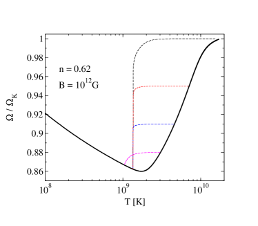
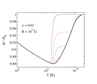
Figure 1: $f$-mode spin-temperature evolution: adapted from Ref. Passamonti et al. (2013), this figure displays the coupled $\Omega-T$ evolution of a Newtonian $n=0.62$ polytropic model with gravitational mass (in the non-rotating limit) $M=1.98\,M_{\odot}$ under the combined influence of an unstable $\ell=m=4$ $f$-mode and magnetic dipole torque. The thick solid curve represents the instability window (accounting for standard shear and bulk viscosity but not for superfluid mutual friction). Left panel: the various evolution trajectories correspond to different initial $\Omega$ and a surface dipole field $B=10^{12}\,\mbox{G}$. Right panel: the same initial $\Omega$ values as before for a surface dipole field $B=10^{13}\,\mbox{G}$.

But before opening the discussion on the $f$-mode instability in relativistic stars it is worth reviewing the recent progress achieved with the use of the “outdated” Newtonian framework. The first problem to be addressed was that of the coupled spin-temperature evolution of a neutron star undergoing an $f$-mode instability Passamonti et al. (2013). Using a formalism similar to that previously employed for the $r$-mode instability Owen et al. (1998), this work considered hot and rapidly rotating newly formed systems entering the instability window as the temperature drops below $\sim 10^{10}\,\mbox{K}$ – this value marks the regime where bulk viscosity becomes negligibly weak. The unstable $f$-mode is promptly saturated, at which point the star begins to spin down with emission of gravitational radiation at almost constant temperature until it exits the instability window.

A representative example of this evolution is shown in Fig. 1 for the most unstable $\ell=m=4$ $f$-mode of a massive $M=1.98\,M_{\odot}$ stellar model with a $n=0.62$ polytropic EOS. A first noteworthy feature of these $f$-mode trajectories is that the system is unlikely to ever enter the region where neutrons pair to form a superfluid phase (this is expected to happen at a temperature $T\lesssim 10^{9}\,\mbox{K}$) and the instability is suppressed by vortex mutual friction. Even more important is the interplay between the stellar magnetic field and the unstable $f$-mode. A neutron star with surface field $B\gg 10^{12}\,\mbox{G}$ will evolve along a shorter spin-temperature trajectory (see right panel of Fig. 1) with its spin evolution mostly driven by the magnetic dipole radiation rather than gravitational radiation, hence leading to a deteriorated GW detectability. A similar situation may arise if in parallel with the $f$-mode there is also an unstable $r$-mode present in the system – a not unlikely scenario given the much wider instability window of the latter, see Ref. Passamonti et al. (2013) for more details.

A second key recent development concerns saturation amplitude (or equivalently saturation energy) of the instability. This arduous calculation was undertaken in Pnigouras and Kokkotas (2015, 2016) by means of a nonlinear mode-coupling model similar to the one that had been employed before for the $r$-modes (see Section V) but with the added property of non-uniform, stratified matter. According to the aforementioned work the mode’s energy is primarily drained by the non-linear coupling to $g$-modes; this leads to a saturation energy that may fluctuate considerably across the instability’s $\Omega-T$ parameter space. A representative maximum value for the saturation energy can be taken to be $E_{\rm sat}\sim 10^{-6}Mc^{2}$ Pnigouras and Kokkotas (2015, 2016). This result has obvious implications for the GW detectability of unstable $f$-modes and will be discussed in more detail below.

IV.2 The $f$-mode instability in relativistic stars: a story of revival?

The last few years have seen a renewed interest in the $f$-mode instability with the objective of revising the earlier Newtonian results using relativistic and rapidly rotating neutron star models. This effort was spearheaded by Ref. Gaertig et al. (2011) which considered polytropic models and relativistic gravity in the Cowling approximation. These first relativistic results were promising, predicting a revised $f$-mode growth timescale about an order of magnitude shorter than the Newtonian value for the same canonical stellar parameters. Accordingly, the instability window was found to be larger than its Newtonian counterpart, with the $\ell=m=4$ being the most unstable multipole, see Fig. 2 (left panel). Follow-up work Doneva et al. (2013) established that the combination of a realistic EOS model with a higher stellar mass ($\approx 2M_{\odot}$) can support an even wider instability window – this is shown on the right panel of Fig. 2 and can be directly compared against the Newtonian window of Fig. 1 (which corresponds to a Newtonian polytrope of the same mass).

These calculations allow us to draw a clear conclusion: for a given rotation $\Omega$, massive relativistic systems (which are also the most compact ones) have significantly enhanced $f$-mode instability properties as compared to their Newtonian and/or less massive counterparts.

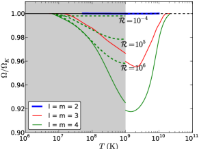
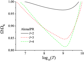
Figure 2: Relativistic $f$-mode instability window. Left panel: this figure, taken from Ref. Gaertig et al. (2011), shows the $f$-mode instability window (solid curves) corresponding to the first three multipoles $\ell=m=2,3,4$ and for a $n=0.73$ relativistic polytrope with parameters $M=1.48M_{\odot}$ and $R=10.47\,\mbox{km}$ (in the $\Omega=0$ limit). The shaded area indicates the parameter space where neutron superfluidity is present (with a fiducial onset temperature $T_{\rm cn}=10^{9}\,\mbox{K}$ ). The critical curves are discontinuous at $T_{\rm cn}$ as a result of the use of different shear viscosity coefficients in the superfluid and normal region. The dashed curves show the instability window of the $\ell=4$ multipole with vortex mutual friction accounted for and the drag coefficient shifted from its canonical value ${\cal R}\approx 10^{-4}$ (which leads to a fully suppressed instability). Right panel: the instability window for the same $f$-mode multipoles (this time assuming non-superfluid matter) and for a neutron star model with a realistic EOS (in this particular example APR) and parameters $M=2M_{\odot}$, $R=10.88\,\mbox{km}$, see Ref. Doneva et al. (2013).

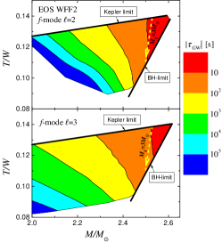
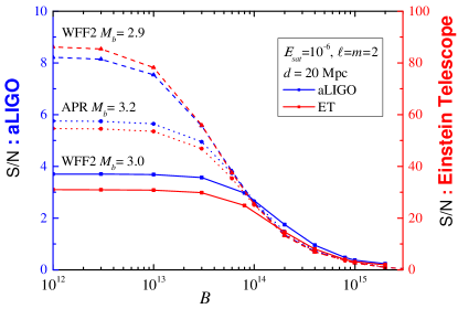
Figure 3: $f$-mode instability in supramassive neutron stars. Left panel: this figure is adapted from Ref. Doneva et al. (2015) and shows the $f$-mode growth timescale (for the first two multipoles and assuming a WFF2 EOS stellar model) as a function of the supramassive neutron star’s mass. Right panel: the GW signal-to-noise ratio as a function of the surface dipole field for a supramassive neutron star located at a fiducial distance $20\,\mbox{Mpc}$, spinning down under the combined influence of the $f$-mode instability (saturated at $E_{\rm sat}=10^{-6}Mc^{2}$) and magnetic dipole radiation, for different choices of baryonic mass and EOS (figure adapted from Doneva et al. (2015)).

The most dramatic manifestation of this conclusion may take place in the immediate aftermath of the merger of a binary neutron star system: for the expected range of initial masses the merger may not immediately produce a black hole but, instead, lead to a transient phase of a supramassive ($M\sim 2.5M_{\odot}$) and $\Omega\approx\Omega_{\rm K}$ neutron star remnant . Besides their central role in GW astronomy, these mergers have come to be seen as the leading theoretical model for the central engine powering short GRBs (see e.g. Dai and Lu (1998); Zhang and Mészáros (2001); Rowlinson et al. (2013)). The supramassive remnant, which now takes the form of a proto-magnetar as a result of strong magnetic field amplification (see e.g. Rezzolla et al. (2011); Kiuchi et al. (2014); Giacomazzo et al. (2015)), is believed to power the burst’s late-time emission and is associated with the X-ray plateau and power-law tail seen in the light curves of several of these events Rowlinson et al. (2013); Metzger and Piro (2014). According to the GRB data, the remnant’s lifetime spans a range $10^{2}-10^{5}\,\mbox{s}$ which is determined by the spin-down timescale due to magnetic dipole radiation (the same mechanism is responsible for powering the system’s X-ray emission).

It is during this X-ray “afterglow”/supramassive phase where the $f$-mode instability is most likely to take place and become a potentially strong source of GWs. Viscosity is not likely to be an impeding factor in these circumstances since the system is expected to cool below $10^{10}\,\mbox{K}$ very shortly after the supramassive remnant has been formed, see e.g. Lasky and Glampedakis (2016). This scenario has been put forward in Ref. Doneva et al. (2015) and is backed up by $f$-mode calculations that suggest surprisingly short growth timescales, $\tau_{\rm gw}\sim 10-100\,\mbox{s}$, see Fig. 3 (left panel). However, a short $\tau_{\rm gw}$ does not necessarily translate into a conspicuous $f$-mode GW signal. To what extent post-merger supramassive remnants could be realistic targets for present and next generation GW detectors is discussed in more detail in the following section.

IV.3 The observability of the $f$-mode instability

The overall amplitude of the $f$-mode signal is limited by the distance of the source and the mode’s maximum saturation amplitude. As we have already seen, the latter parameter was recently obtained and expressed as a saturation energy, $E_{\rm sat}\sim 10^{-6}Mc^{2}$ Pnigouras and Kokkotas (2015, 2016). A perhaps more intuitive way to quantify this result is via the $f$-mode-induced ellipticity in the stellar shape. A back-of-the-envelope calculation leads to Lasky and Glampedakis (2016),

$$\frac{\delta R}{R}\sim\left(\frac{E_{\rm sat}}{Mc^{2}}\right)^{1/2}\left(\frac{cR}{GM}\right)^{1/2},$$ (19)

which for a typical neutron star compactness returns $\delta R/R\sim 10^{-3}$. In other words, the mode gets saturated at a “linear” level. The GW observability of an unstable $f$-mode saturated at this maximum amplitude is shown in Fig. 3 (right panel) in the form of a signal-to-noise ratio (SNR) for the Advanced LIGO/Virgo and ET detectors as a function of the surface dipole field Doneva et al. (2015). Detectability is strongly diminished in systems with magnetar-like fields for the simple reason that the spin-down timescale is controlled by magnetic dipole radiation and is much shorter than the duration of a GW-driven spin-down (see also Fig. 1). Less magnetised systems with $B\lesssim 10^{14}\,\mbox{G}$ are likely to be marginally detectable by Advanced LIGO but should be “in the bag” for ET.

A more empirical assessment of the $f$-mode’s GW observability can be made with the help of the short GRB X-ray data Lasky and Glampedakis (2016). The $\sim t^{-2}$ late time decay profile seen in several light curves of these events can be taken as evidence of an electromagnetic radiation dominated spin-down, in accordance with the GRB proto-magnetar model. This information, in combination with the observed duration of the X-ray plateaus, can be used to set upper limits in the saturation amplitude of unstable $f$-modes. Interestingly, the resulting limit is similar to the theoretically predicted maximum amplitude – this result suggests that the $f$-mode instability could in principle play an important role in the dynamics of the post-merger remnant. Unfortunately, the predicted $f$-mode detectability is rather pessimistic even for ET, limited by the shortness of the spin-down timescale and the large distances ($\gtrsim 500\,\mbox{Mpc}$) associated with short GRBs.

IV.4 Future directions

The $f$-mode calculations discussed in the preceding sections were carried out using the Cowling approximation. We have already pointed out in a previous section how this approximation affects the $f$-mode asteroseismology formalism. As far as the $f$-mode instability is concerned, it is known Zink et al. (2010); Yoshida (2012) that the Cowling approximation makes relativistic stars less prone to the CFS instability by increasing the rotation threshold (14). It is therefore expected that the $f$-mode instability in neutron star models with fully relativistic dynamical spacetime will be enhanced but a detailed quantitative calculation of this modification is still lacking.

Another desideratum in this area should be the further improvement in the modelling of the $f$-mode’s non-linear saturation physics. The very recent state-of-art calculation of Pnigouras and Kokkotas (2015, 2016) is “primitive” in the sense that it is based on a Newtonian framework and a slow rotation approximation. Taking this calculation to the next level (with relativistic gravity and/or fast rotation) is likely to prove a very challenging – but necessary – endeavour.

Finally, it should be borne in mind that the $f$-mode instability window could be significantly modified by viscosity due to the presence of exotic phases of matter in the interior of neutron stars, such as hyperons and quarks. Although this scenario has been exhaustively explored in the context of the $r$-mode instability (see Section V) very little is known about its impact on the $f$-mode instability.

V The $r$-mode instability

The discovery of the inertial $r$-mode CFS instability in 1998 came as something of a surprise to the neutron star community Andersson (1998); Friedman and Morsink (1998). Since then this instability has received the lion’s share of the published work on the subject of neutron star oscillations as a consequence of its potentially key role in the spin evolution of neutron stars and as a promising source of GWs (for early comprehensive reviews on the subject see Andersson and Kokkotas (2001); L. and Stergioulas (2013); a more specialised recent review can be found in Haskell (2015)). Accordingly, this $r$-mode section occupies a central place in this review.

Two key characteristics are associated with the $r$-mode instability:

(i) the mode frequency in the rotating frame is

$$\omega_{r}=\frac{2m\Omega}{\ell(\ell+1)},$$ (20)

so that with dissipation switched off, the mode becomes CFS-unstable as soon as the star acquires rotation (that is, the condition (14) is automatically satisfied for any $\Omega$). With dissipation restored, the resulting $\Omega-T$ instability window is in general quite large.

(ii) the mode’s predominant axial geometry implies a nearly horizontal fluid flow pattern and leads to GW emission dominated by the current multipole ${\cal S}_{22}$ rather than the mass multipoles. The resulting growth timescale $\tau_{\rm gw}$ exhibits a characteristic $\sim\Omega^{-6}$ dependence and is very short. For a canonical $n=1$ Newtonian polytropic star this is Lindblom et al. (1998); Andersson and Kokkotas (2001),

$$\tau_{\rm gw}\approx 50\,M_{1.4}^{-1}R_{6}^{-4}P_{-3}^{6}\,\mbox{s}.$$ (21)

The two above properties alone are sufficient to guarantee the astrophysical relevance of the $r$-mode instability. In addition, practitioners of neutron star dynamics enjoy the luxury of being able to do most of $r$-mode physics within a Newtonian/slow rotation framework rather than having to struggle with the complexity of rapidly rotating GR stars (as it was the case for the $f$-mode instability). Nonetheless, relativistic $r$-mode calculations have been performed Lockitch et al. (2001); Ruoff and Kokkotas (2001); Yoshida and Lee (2002); Lockitch et al. (2003); Idrisy et al. (2015) and have demonstrated the corrections to the Newtonian mode eigenfunction GW growth timescale to be typically very small. At a qualitative level, GR changes the purely axial slow-rotation Newtonian $r$-mode into an axial-led inertial mode – this is similar to the modification caused by fast rotation in Newtonian theory. More pronounced is the relativistic correction to the mode frequency which is of the order of $\sim 20\%$. This is large enough to be accounted for in searches for GW signals from unstable $r$-modes Owen (2010). The $r$-mode’s insensitiveness extends to variations in the EOS of matter as well. This has been demonstrated by the very recent analysis of Idrisy et al. (2015) and is in agreement with earlier investigations that made use of polytropic models Lockitch et al. (2003). The upshot is that $r$-mode calculations based on a canonical polytropic Newtonian model (or even a uniform density model) are sufficiently robust and accurate for most practical applications. This will be our benchmark model for the reminder of our discussion of the $r$-mode instability unless otherwise specified.

V.1 $r$-mode phenomenology

Most of the uncertainty related to the $r$-mode instability has to do with its damping. In a “minimum physics” (although not necessarily realistic!) model that assumes dissipation only due to standard shear and bulk viscosity the resulting instability window overlaps with the box-shaped region occupied by the known population of rapidly rotating neutron stars in LMXBs and MSPs. This $r$-mode window is shown in Fig. 4, where we have also included LMXB data tabulated in Mahmoodifar and Strohmayer (2013); Ho et al. (2011) (to be discussed below). The striking feature of Fig. 4 is that several known neutron stars reside well inside the minimum damping window and therefore should harbour unstable $r$-modes. This observation forms the basis of what we shall call the “$r$-mode puzzle” in the following section.

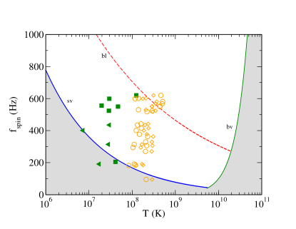
Figure 4: $r$-mode instability window. This figure shows the $r$-mode spin-temperature instability window (in terms of the spin frequency $f_{\rm spin}=\Omega/2\pi$) assuming a canonical neutron star model and accounting for standard shear (blue curve) and bulk (green curve) viscosity. The corresponding viscous damping timescales were taken from Lindblom et al. (1998) and Andersson and Kokkotas (2001) while Eq. (21) was used for the growth timescale. The shaded area represents the region of $r$-mode stability. Besides the minimum damping window, the figure also includes the critical curve due to Ekman boundary layer damping (red dashed curve) which is discussed in Section V.6. The data points represent LMXBs with known spin frequencies. The core temperature is inferred by flux measurements during phases of quiescence Mahmoodifar and Strohmayer (2013) (filled squares and triangles for upper limits) or is theoretically predicted assuming a combined $r$-mode spin and thermal equilibrium during phases of accretion Ho et al. (2011) (open diamonds and circles for cooling dominated by mURCA reactions and Cooper pair processes respectively) see Section V.3 for details.

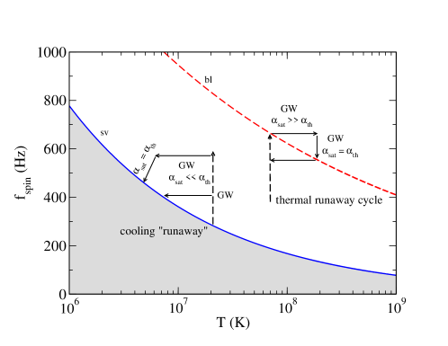
Figure 5: $r$-mode spin-temperature evolution. The $r$-mode-driven $f_{\rm spin}-T$ evolution of an accreting neutron star is determined by (i) the instability curve’s slope at the point where the system, spun up by accretion, first enters the instability window (dashed vertical lines) and (ii) the maximum saturation amplitude $\alpha_{\rm sat}$. In this figure we show the canonical scenario of a negative slopping instability curve due to shear viscosity (blue curve) or an Ekman layer (red curve). If the saturation amplitude is not too small ($\alpha_{\rm sat}\gg\alpha_{\rm th}$ initially), the system is forced into a cyclic thermal runaway loop in the vicinity of the instability curve where the GW emitting portions are indicated in the figure, see Sections V.1 & V.3 for more details. The cycle’s nearly horizontal path ($r$-mode heating) continues until thermal equilibrium is established, $\alpha_{\rm sat}=\alpha_{\rm th}$, followed by $r$-mode spin-down towards the instability curve. In the opposite scenario of a very small saturation amplitude (i.e. $\alpha_{\rm sat}\ll\alpha_{\rm th}$ initially) a weak $r$-mode instability is active during accretion and, once the latter has ended, cannot prevent the system from cooling (at nearly constant spin) towards a state of thermal equilibrium or until the instability curve is crossed again (this scenario is shown here with respect to the minimum damping curve).

The spin distribution of these neutron stars has been something of a mystery since under the unhindered action of accretion, LMXBs (and their MSP descendants) should have been expected to straddle the Kepler frequency limit, $f_{\rm K}\gtrsim 1\,\mbox{kHz}$ (see also e.g. the discussion in Haskell et al. (2012)). The apparent spin cut-off at a much lower frequency has been taken as evidence of the presence of a spin-down torque that counteracts accretion. A suggestion that has attracted much attention since its conception is that of a GW torque supplied either by a deformation in the stellar shape (i.e. a neutron star “mountain”) or an unstable oscillation mode Papaloizou and Pringle (1978); Bildsten (1998a); Andersson et al. (1999). This idea obviously combines well with the minimum dissipation $r$-mode model but we should not be too hasty in drawing conclusions. Spin equilibrium in LMXBs could be achieved by an alternative non-GW mechanism, namely, the coupling of the stellar magnetic field with the accretion disk Ghosh and Lamb (1979); Wang (1995); Rappaport et al. (2004); Andersson et al. (2005b) and it is here fitting to open a parenthesis and discuss it.

In the disk coupling model the global stellar magnetic field threads the material of the disk and the field lines, being simultaneously anchored in the disk and on the stellar surface, provide a very efficient braking mechanism. With the input of canonical surface dipole fields, $B\sim 10^{8}-10^{9}\,\mbox{G}$, and reasonable physical assumptions the predictions of the available phenomenological disk coupling models compare fairly well with LMXB spin data Andersson et al. (2005b); Haskell and Patruno (2011); Patruno and Watts (2012) thus dispelling much of the mystery behind their spin distribution cut off . Although this is compelling evidence in favour of these models it is certainly premature to shelve the alternative GW-based mechanisms. In fact, recent work Bhattacharyya and Chakrabarty (2017); Bhattacharyya (2017) suggests that the transient nature of accretion could seriously weaken the efficiency of the disk coupling model thus calling for an additional spindown torque. What can be said with certainty is that the existing data do not exclude the realistic possibility of having some $r$-mode activity (or indeed a neutron star mountain) in LMXB systems that could otherwise be dominated by magnetic disk coupling or by magnetic dipole spin-down when in quiescence. The disk coupling model does, however, remove the need to cling to solely GW-based spin equilibrium models. With this observation in mind we can resume our main $r$-mode discussion.

Once inside the instability window, the $r$-mode drives a coupled spin-temperature evolution the details of which are largely determined by the maximum (saturation) value of the mode amplitude $\alpha_{r}$. This dimensionless parameter is commonly defined in the literature via the velocity field of the dominant $\ell=m$ mode Owen et al. (1998)

$$\delta\mathbf{v}=\alpha_{r}\left(\frac{r}{R}\right)^{\ell}\Omega R\mathbf{Y}_{\ell\ell}^{B}e^{i\omega_{r}t},$$ (22)

where $\mathbf{Y}_{\ell m}^{B}$ is a vector spherical harmonic of the magnetic type. More simply, we can think of the amplitude as the ratio $\alpha_{r}\approx\delta v/\Omega R$.

Considering first accreting neutrons stars, once the system moves across a $d\Omega/dT<0$ segment of the instability curve during spin up it will undergo a cyclic thermal runaway Levin (1999); Andersson et al. (2000); Bondarescu et al. (2007), see Fig. 5.

The cycle begins with the mode growing under the emission of gravitational radiation, rapidly reaching its maximum saturation value $\alpha_{\rm sat}$. When this happens, and assuming $\alpha_{\rm sat}\ll 1$, the viscous timescale becomes comparable to the growth timescale, $\tau_{\rm visc}\approx\tau_{\rm gw}$, (see the $r$-mode evolution equations in Owen et al. (1998); Levin (1999)). At the same time the heat deposited by shear viscosity lifts the stellar core temperature. This happens at almost constant spin frequency since the GW spin-down timescale, $\tau_{\rm sd}^{\rm gw}\equiv\Omega/|\dot{\Omega}|$, is always much longer than the heating timescale $\tau_{\rm heat}\equiv T/|\dot{T}|$. These timescales are (see e.g. Levin (1999)):

$$\tau_{\rm sd}^{\rm gw}\approx\frac{5.3}{\alpha_{\rm sat}^{2}}\tau_{\rm gw},\qquad\tau_{\rm heat}=\frac{C_{\rm v}T}{\dot{E}_{\rm visc}}\approx 7.8\times 10^{-6}\,\frac{P_{-3}^{2}\,T_{8}^{2}}{\alpha_{\rm sat}^{2}M_{1.4}R_{6}^{2}}\,\tau_{\rm gw}.$$ (23)

where in the last equation the damping rate $\dot{E}_{\rm visc}$ is typically fixed by shear viscosity or a crust-core boundary layer (see below) and the heat capacity $C_{\rm v}\approx 1.4\times 10^{38}\,T_{8}\,\mbox{erg}/\mbox{K}$ is that of ordinary matter Shapiro and Teukolsky (1986) (superfluidity would reduce $\tau_{\rm heat}$ even further by decreasing $C_{\rm v}$). Also note that we have explicitly used the timescale equality $\tau_{\rm visc}\approx\tau_{\rm gw}$ for a saturated mode.

The thermal runaway continues up to the point where stellar cooling can efficiently balance viscous heating. Assuming neutrino cooling due to the standard modified URCA process (with the corresponding emissivity $L_{\nu}\approx 7\times 10^{31}\,T_{8}^{8}\,\mbox{erg}/\mbox{s}$) Shapiro and Teukolsky (1986) and a minimum damping instability curve, we can convert thermal equilibrium into a “thermal” $r$-mode amplitude,

$$\dot{E}_{\rm visc}=\dot{E}_{\rm sv}=L_{\nu}~{}\Rightarrow~{}\alpha_{\rm th}\approx 1.4\times 10^{-9}M_{1.4}^{-1}R_{6}^{-3}P_{-3}^{4}T_{8}^{4}.$$ (24)

Note that this result is indicative as it obviously depends on the assumed cooling physics. For the temperature range of LMXBs the cooling could be dominated by superfluid Cooper-pair processes Ho et al. (2011) or even surface photon emission Mahmoodifar and Strohmayer (2013).

At the stage of thermal equilibrium the temperature remains essentially constant and the $r$-mode-driven spin-down steers the system towards the instability curve; once the curve is crossed, the star becomes stable again and rapidly cools. Eventually, accretion will once again spin up the star preparing the ground for the next cycle. The duration of the GW-emitting portion of this cycle depends on $\alpha_{\rm sat}$. A large amplitude (the first papers to explore the implications of this $r$-mode evolution were somewhat optimistically assuming $\alpha_{\rm sat}\sim 0.1-1$, see e.g. Andersson et al. (2000)]) translates to fast GW-driven evolution but a tiny GW duty cycle, making LMXBs uninteresting sources of GWs. If $\alpha_{\rm sat}$ is small, the system does not wander off much from the instability curve and the cycle’s GW efficiency can improve dramatically. We can make this argument quantitative by approximating the cycle’s GW efficiency as the ratio between the time the system spends emitting radiation and the typical LMXB lifetime Heyl (2002),

$$D_{\rm cycle}\approx\frac{t_{\rm cycle}}{10^{7}\,\mbox{yr}}\approx\frac{10^{-11}}{\alpha_{\rm sat}^{2}}.$$ (25)

Combining this with the estimated LMXB birth rate $\sim 10^{-5}/\mbox{yr}/\mbox{galaxy}$, it is not too difficult to see that in order to have a system always switched on in our Galaxy,

$$D_{\rm cycle}\lesssim 10^{-2}~{}\Rightarrow~{}\alpha_{\rm sat}\lesssim 10^{-4}.$$ (26)

Thus, somewhat counterintuitively, a relatively small amplitude is likely to improve the $r$-mode’s GW detectability in LMXBs. Of course, the amplitude should not be too small for otherwise these sources would be too faint. As discussed below, the upper limit (26) is compatible with the theoretically predicted $r$-mode saturation amplitude.

In the thermal runaway scenario described above the cut off in the spin distribution of LMXBs is set by the spin frequency at which the systems enter the instability window. Taking into account that the expected temperature range for LMXBs is $T\sim 10^{7}-5\times 10^{8}\,\mbox{K}$ it becomes immediately clear that the previously defined minimum damping window is in disagreement with the observed $\sim 600\,\mbox{Hz}$ cut off (see Fig. 4). The model does much better if we invoke a “canonical” $r$-mode instability window which, in addition to shear and bulk viscosity, accounts for dissipation due to a viscous Ekman boundary layer at the crust-core boundary. The implications of this Ekman layer could be crucial for the survivability of the $r$-mode instability and are discussed in detail below in Sections V.6 & V.7.

It should also be emphasised that the cyclic evolution is not an unavoidable outcome of the $r$-mode evolution in LMXBs. For instance, the presence of exotic neutron star matter in the form of hyperons or quarks could lead to an instability curve with positive $d\Omega/dT$ slope in the temperature range relevant to LMXBs. As discussed by several authors, this configuration could effectively trap accreting systems near the critical curve and turn them into persistent sources of GWs Andersson et al. (2002); Nayyar and Owen (2006); Haskell and Andersson (2010). Another way to prevent the cyclic evolution from happening is by invoking a saturation $\alpha_{\rm sat}$ sufficiently small so that $\tau_{\rm heat}$ (and consequently $\tau_{\rm sd}^{\rm gw}$) exceeds the accretion timescale ($\sim 10^{7}-10^{8}\,\mbox{yr}$). In this scenario cooling dominates over $r$-mode heating, i.e. $\alpha_{\rm sat}\ll\alpha_{\rm th}$, and once accretion comes to an end the system undergoes a “cooling runaway”, moving towards the low $T$ part of the instability window until thermal equilibrium is established or the instability curve is crossed Alford and Schwenzer (2015), see Fig. 5. We elaborate more on this small amplitude scenario below in Section V.3.

The $r$-mode-driven evolution of rapidly rotating non-accreting neutron stars is somewhat simpler than the cyclic scenario of the preceding paragraphs. These systems can be either old MSPs or, more speculatively, very young neutron stars such as the central compact objects (CCOs) associated with supernova remnants. The latter objects have already been the target of broad band GW searches by LIGO and, in spite of their unknown spin frequencies (which are likely to be low), have led to direct upper limits on the $r$-mode amplitude Aasi et al. (2015). The key parameter here is the spin-down timescale (23) which becomes

$$\tau_{\rm sd}^{\rm gw}\approx 800\,\left(\frac{10^{-4}}{\alpha_{\rm sat}}\right)^{2}M_{1.4}^{-1}R_{6}^{-4}P_{-3}^{6}\,\mbox{yr}.$$ (27)

According to this expression, a large amplitude $r$-mode drives a very rapid spin-down thus seriously diminishing the system’s GW observability. In order to have a $\tau_{\rm sd}^{\rm gw}$ that is compatible with the estimated ages of the CCOs (i.e. $\sim 10^{2}-10^{3}\,\mbox{yr}$) we would need to invoke $\alpha_{\rm sat}\sim 10^{-3}$. A much smaller amplitude is required if $\tau_{\rm sd}^{\rm gw}$ is associated with the observed spin-down age of MSPs. We will return to this point later, in Section V.3.

V.2 An $r$-mode puzzle?

How do actual observations compare against the basic $r$-mode phenomenology described in the preceding section? As we have seen, the minimum damping model clearly predicts that the $r$-mode instability should be operating in a large portion of the LMXB and MSP populations (and perhaps in some young sources). The fact that these objects do not appear to show any evidence of strong $r$-mode activity should have important implications for the physics in their interior. For example, and as already pointed out, the data points shown in Fig. 4 are clearly incompatible with a thermal runaway cycle taking place near the standard shear viscosity instability curve. Similarly, the MSP timing data are incompatible with the $r$-mode instability unless $\alpha_{\rm sat}$ is very small.

A clue is provided by the observed long-term spin-down of accreting millisecond X-ray pulsars (AMXPs) in quiescence (see Patruno and Watts (2012) for a review). For example, two of these objects, SAX J1808-3658 and IGRJ00291+5934, are likely to sit inside the instability window (given the uncertainties on the pulsar parameters), and therefore could experience $r$-mode-driven spin-down. However, the measured spin-down rate is consistent with that caused by a canonical LMXB magnetic field ($\sim 10^{8}\,\mbox{G}$), hence suggesting that the $r$-mode instability is not the dominant effect here Haskell and Patruno (2011); Pappito et al. (2011).

This apparent tension between the minimum damping $r$-mode model and the spin-temperature data of known rapidly rotating neutron stars may be dubbed the “$r$-mode puzzle”.

There are two complementary ways to make theory and observations mutually compatible. The first one relies on the presence of additional damping mechanisms that could modify the instability window and render $r$-mode-stable the systems in question. The required extra damping could be provided, for example, by exotic matter in the neutron star core, strong superfluid vortex mutual friction or an Ekman-type viscous boundary layer at the crust-core interface. The second possibility is that of a small saturation amplitude $r$-mode. In this scenario the $r$-mode instability does operate in (at least) some rapidly rotating neutron stars but $\alpha_{\rm sat}$ is sufficiently small so that the ensuing sluggish $r$-mode evolution is compatible with observations. We now can take a closer look at these two resolutions of the $r$-mode puzzle.

V.3 Small amplitude $r$-modes

Theoretical calculations already provide constraints on $\alpha_{\rm sat}$ and obviously need to be incorporated in any realistic $r$-mode model. The most robust saturation mechanism is provided by non-linear couplings between the $r$-mode and other (primarily inertial) modes Schenk et al. (2002); Arras et al. (2003); Bondarescu et al. (2007, 2009). A series of impressive tour de force calculations have revealed a complicated spin-temperature evolution pattern for $\alpha_{\rm sat}$ but as a rule of the thumb estimate for the time-averaged amplitude we can take $\alpha_{\rm sat}\sim 10^{-4}-10^{-3}$ Schenk et al. (2002); Arras et al. (2003); Bondarescu et al. (2007, 2009).

This level of saturation is obviously low but not low enough for the purposes of the small amplitude scenario! To illustrate this, we consider MSPs with measured spin-down rates that reside inside the minimum damping instability window. These data can be used to set upper limits on the $r$-mode amplitude (obviously, these limits make sense provided the systems in question are $r$-mode-unstable in the first place – this may not be the case in a more realistic enhanced damping scenario). Equating the total rate of change of the stellar rotational energy to the GW torque leads to a spin-down $r$-mode amplitude (see e.g. Owen (2010)) :

$$\alpha_{\rm sd}\approx 5.7\times 10^{-3}P^{5/2}_{-3}\dot{P}_{-10}^{1/2}M_{1.4}^{-1/2}R_{6}^{-2}.$$ (28)

The strongest constraints from the available MSP data imply a very small amplitude, $\alpha_{\rm sd}\lesssim 10^{-7}$ Alford and Schwenzer (2014a, 2015).

Given that MSPs are almost certainly spinning down via standard magnetic dipole radiation, it is meaningful to compare the relative $\dot{P}$ contribution of GW emission. It is an easy exercise to derive the following formula for the spin-down ratio $\dot{P}_{\rm gw}/\dot{P}_{\rm em}$ which is also equal to the spin-down age ratio $\tau_{\rm sd}^{\rm em}/\tau^{\rm gw}_{\rm sd}$:

$$\frac{\dot{P}_{\rm gw}}{\dot{P}_{\rm em}}=\frac{\tau_{\rm sd}^{\rm em}}{\tau^{\rm gw}_{\rm sd}}\approx 0.23\left(\frac{\alpha_{r}}{10^{-7}}\right)^{2}M_{1.4}^{2}B_{8}^{-2}P_{-3}^{-4}.$$ (29)

This expression indeed verifies that for canonical MSP parameters the $r$-mode torque is much weaker than the electromagnetic one.

Two more key $r$-mode amplitudes can be calculated by making contact with LMXB observations. The first one comes from the assumption of spin equilibrium (discussed earlier). Using a simple fiducial spin up torque that ignores the effect of the magnetic field on the accretion dynamics leads to Brown and Ushomirsky (2000)

$$\alpha_{\rm acc}\approx 1.2\times 10^{-8}\left(\frac{L_{\rm acc}}{10^{35}\,\mbox{erg}\,\mbox{s}^{-1}}\right)^{1/2}P_{-3}^{7/2}$$ (30)

where $L_{\rm acc}$ is the accretion luminosity. This estimate is very close to the spin equilibrium amplitude obtained in Ref. Mahmoodifar and Strohmayer (2013) using a spin-up torque extracted observationally from the time-averaging over a succession of accretion episodes.

The second “handle” for estimating $r$-mode amplitudes is provided by the consideration of thermal equilibrium in LMXBs Ho et al. (2011); Mahmoodifar and Strohmayer (2013). Measuring the luminosity of these objects in quiescence allows the inference of their surface and core temperature and in turn of their cooling rate. If heating is attributed to the dissipation of a steady-state unstable $r$-mode, the mode amplitude can be calculated by invoking thermal equilibrium. This is the approach taken in Mahmoodifar and Strohmayer (2013) and is of the same logic that led to the amplitude (24).

The quiescent LMXBs considered in Mahmoodifar and Strohmayer (2013) have $T\lesssim 10^{8}\,\mbox{K}$ (see data points in Fig. 4) – this implies a cooling dominated by surface photon emission rather that neutrinos. The resulting thermal equilibrium amplitudes lie in the range $\alpha_{\rm th}\sim 10^{-8}-10^{-7}$. A closer look at the tabulated data of Mahmoodifar and Strohmayer (2013) reveals that for sources with both spin and thermal equilibrium data $\alpha_{\rm th}\approx 0.1\alpha_{\rm acc}$. This means within the minimum damping model, and treating the inferred $\alpha_{\rm th}$ as an empirical saturation amplitude, $r$-modes cannot balance the long-term accretion torque in LMXBs. Furthermore, using $\alpha_{\rm th}$ in Eq. (29) we find $\dot{P}_{\rm gw}\ll\dot{P}_{\rm em}$. In other words, quiescent LMXBs are expected to predominantly spin-down via magnetic dipole radiation, in agreement with observations Haskell and Patruno (2011).

A different angle of approach that makes more contact with the accreting phase of LMXBs rather that their quiescence assumes both $r$-mode thermal and spin equilibrium to take place at the same time. Then, the equality $\alpha_{\rm acc}=\alpha_{\rm th}$ relates $T$ to the observables $L_{\rm acc}$ and $P$. As shown in Ho et al. (2011) the LMXB core temperatures calculated in this way lie in the range $T\sim 10^{8}-5\times 10^{8}\,\mbox{K}$ and are consistently higher than those in Mahmoodifar and Strohmayer (2013) (see also Fig.  4). Of course this model would run into difficulties in explaining the quiescence data (at least for some systems).

What is noteworthy from the preceding discussion is that the three “observable” amplitudes $\alpha_{\rm sd},\alpha_{\rm acc},\alpha_{\rm th}$ lie well below the predicted $\alpha_{\rm sat}$ due to non-linear couplings. This is clearly problematic from a theoretical point of view and therefore other saturation mechanisms must be sought in order to fill the gap. A recently suggested alternative mechanism is based on the dissipative coupling between the superfluid vortex array and the quantised magnetic fluxtubes in regions of the star where a neutron superfluid co-exists with a proton superconductor Haskell et al. (2014). The resulting saturation amplitude could be as small as $\alpha_{\rm sat}\sim 10^{-5}-10^{-6}$. Although this is much smaller than the mode-coupling $\alpha_{\rm sat}$, there is still some significant difference with the observable amplitudes.

The small $r$-mode amplitude scenario has been further explored in a recent series of papers by Alford & Schwenzer Alford and Schwenzer (2014b, a, 2015). Following an analysis similar to that of Bondarescu et al. (2007, 2009) but allowing for a very small $\alpha_{\rm sat}(\Omega,T)$, they derive steady-state $r$-mode evolution trajectories for LMXBs/MSPs and young neutron stars. As mentioned earlier, in their model the cyclic thermal runaway in accreting systems does not take place since the $r$-mode is too feeble to heat up (or spin down) the star efficiently. After the end of accretion, the system simply cools until it reaches a steady state at a lower temperature (see Fig. 5). This scenario, however, cannot explain the cut off in the LMXB spin distribution since, in the absence of any other spin-down mechanism, these systems would be free to reach the Kepler limit.

At this point it is worth pausing to consider the actual GW detectability of $r$-mode-active neutron stars as a function of the amplitude and the spin frequency.

V.4 $r$-mode detectability

Given the broad scope of this review, the discussion of the $r$-mode’s detectability will necessarily be brief – a more detailed recent analysis can be found in Kokkotas and Schwenzer (2016). The intrinsic GW strain associated with an $r$-mode can be computed with the help of Thorne’s multipole moment formula Thorne (1980). The contribution of the dominant $\ell=m=2$ current multipole is (see e.g. Owen (2010)):

$$h_{0}\approx 4\times 10^{-23}\,\alpha_{r}M_{1.4}R_{6}^{3}\left(\frac{1\,\mbox{kpc}}{D}\right)\left(\frac{f_{\rm gw}}{100\,\mbox{Hz}}\right)^{3}$$ (31)

where we have normalised the distance $D$ to a galactic source and used the equality between the GW frequency and the mode’s inertial frame frequency,

$$f_{\rm gw}=|f_{\rm mode}|=\frac{4}{3}f_{\rm spin}.$$ (32)

The detectability of the strain (31) is shown in Fig. 6 assuming a one year phase-coherent observation and a source at $D=1\,\mbox{kpc}$. First of all, the smallness of the $r$-mode amplitude essentially eliminates extragalactic sources from being candidate targets for detection unless the source is located within our local group and the amplitude is much higher than the upper limits suggested by LMXB/MSP spin-down and thermal data. This could be a realistic possibility if the systems from which the data came from are not $r$-mode unstable – in that case it would make sense to use a fiducial amplitude $\alpha_{r}=10^{-3}$, corresponding to a maximum saturation amplitude due to non-linear mode couplings. The GW strain for this optimistic scenario could indeed be detectable by Advanced LIGO/Virgo (for sources located anywhere in the Galaxy) and of course by ET for sources located further way or rotating at a lower frequency, see Fig. 6. Such $r$-mode signals could be associated with very young neutron stars with still undepleted fast rotation (i.e. fast spinning CCOs), see discussion at the end of Section V.1.

Taking at face value the aforementioned LMXB/MSP upper limits, the amplitude is constrained to be $\alpha_{r}\lesssim 10^{-7}$ and we can see that the prospects for detection of any $r$-mode signal look rather bleak. Only a next generation instrument like ET could score a detection provided the source is rapidly rotating and relatively close ($D\sim 1\,\mbox{kpc}$).

Assuming a neutron star source with known spin frequency, the identification of an $r$-mode signal would be unmistakable due to the $f_{\rm gw}-f_{\rm spin}$ relation (32) which is unique among the various neutron star GW emission mechanisms. Making a source parameter estimation through the GW measured $f_{\rm mode}$ requires the use of the fully relativistic $r$-mode frequency. To leading post-Newtonian order, the correction to the Newtonian frequency comes from the combined effect of gravitational redshift and frame dragging and is of the order of the stellar compactness $M/R$; for a neutron star this translates to an appreciable $\sim 20\%$ frequency shift. With relativistic corrections accounted for, an $r$-mode GW detection would thus lead to a measurement of the compactness.

The importance of using the fully relativistic $r$-mode frequency was recently exemplified by the oscillation discovered in the light curve of a burst from the AMXP XTE 1751-305 Strohmayer and Mahmoodifar (2014). The observed frequency is close to the expected Newtonian $r$-mode frequency for this neutron star’s known spin frequency but an exact match for reasonable stellar mass and radius parameters is only possible if relativistic corrections are taken into account Andersson et al. (2014). Unfortunately, the inferred $r$-mode amplitude is too large to be reconciled with the system’s spin evolution, a result that hints at a different interpretation of the observed oscillation.

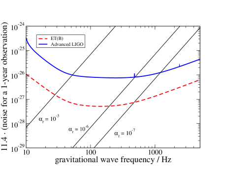
Figure 6: $r$-mode GW detectability. We show the $r$-mode strain (31) assuming a one-year Advanced LIGO/ET phase-coherent observation. For the source parameters we have set $M_{1.4}=1,R_{6}=1.2,D_{1}=1$. The detector noise curves were taken from LIG ; ETc . The three selected mode amplitudes represent approximate upper limits (discussed in the main text) for saturation due to (i) non-linear mode couplings ($\alpha_{r}=10^{-3}$), (ii) spin equilibrium in LMXBs ($\alpha_{r}=10^{-6}$) and (iii) MSP spin-down and thermal equilibrium in LMXBs ($\alpha_{r}=10^{-7}$).

V.5 Beyond the minimum damping model

The alternative scenario of enhanced damping can be seen as a pessimistic standpoint as it attempts to resolve the $r$-mode puzzle by invoking a much reduced instability parameter space that prevents much of the known rapidly rotating neutron stars from becoming $r$-mode active. With regard to the realism of this scenario, it can be safely stated that none of the additional damping mechanisms mentioned earlier (exotic matter, mutual friction, Ekman layer) can be ruled out given our present level of understanding (or ignorance!).

The situation is particularly murky when it comes to exotic matter. For example, the presence of hyperons in neutron star cores and their strong bulk viscosity was once thought to be lethal for the $r$-mode instability Jones (2001); Lindblom and Owen (2002). The day was saved by the likely superfluidity of these particles that effectively shuts down their viscosity below a temperature $\sim 10^{9}\,\mbox{K}$, see e.g. Nayyar and Owen (2006); Haskell and Andersson (2010).

The degree of uncertainty is even higher when it comes to strange quark matter with the resulting instability windows being extremely sensitive to the details of quark pairing, see e.g. Madsen (1998, 2000). More recent work Mannarelli et al. (2008); Andersson et al. (2010) focused on the multifluid aspect of strange stars with colour-flavor-locked paired quark matter and established that the $r$-mode instability suffers very little damping in this type of stars. Unfortunately, given that the very existence (let alone key properties such as viscosity and pairing) of such exotic phases of matter in neutron stars is still a matter of debate, we presently cannot make any reliable prediction.

In our view, it makes more sense to focus on damping mechanisms that rely on less exotic physics. For instance, taking the commonly accepted view that the outer core of mature neutron stars contains a mixture of superfluid neutrons and superconducting protons, the presence of vortex mutual friction is unavoidable. The standard (that is, best understood) form of this type of friction originates from the scattering of electrons by the superfluid’s magnetised vortices and it has been shown to have a negligible effect on $r$-modes Lindblom and Mendell (2000). However, additional mutual friction may originate from the direct interaction between the vortices and the magnetic fluxtubes threading the superconductor, see e.g. Ruderman et al. ; Link (2003). Our understanding of this mechanism is (at best) rudimentary, so far having been used in $r$-mode saturation amplitude calculations Haskell et al. (2014). A more phenomenological approach to this problem is to consider the standard form for the mutual friction force and explore its impact on the $r$-mode by artificially increasing its strength Haskell et al. (2009), see Fig. 7. It is then found that a factor $\sim 100$ increase in the mutual friction drag parameter is sufficient for suppressing the $r$-mode instability in a large portion of the parameter space. Vortex-fluxtube interactions could well lead to friction of this magnitude but more work is required in order to make a safe prediction.

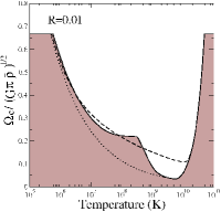
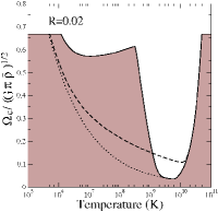
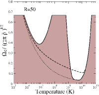
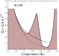
Figure 7: $r$-mode instability window with phenomenological mutual friction. This figure represents the “strong superfluidity” model of Ref. Haskell et al. (2009) and shows the impact that an increasingly amplified vortex mutual friction force would have on the $r$-mode instability window. Note that standard mutual friction (electron scattering by vortices) has a drag coefficient ${\cal R}\sim 10^{-4}$ and leads to negligibly small $r$-mode damping. A much higher ${\cal R}$ could result from vortex-fluxtube interactions. The figure also shows instability curves (for a canonical stellar model) due to standard shear and bulk viscosity as well as due to a slippage-modified Ekman layer (dashed curve).

An entirely different kind of effect, taking place in superfluid neutron stars, could modify the $r$-mode instability’s parameter space Gusakov et al. (2014a, b). In general superfluid matter with two fluid degrees of freedom supports twice as many oscillation modes as compared to ordinary matter. For $r$-modes in particular, this doubling leads to “ordinary” and “superfluid” modes, the real physical distinction between them being the relative amplitude of the two fluids’ co-moving and counter-moving degrees of freedom. The ordinary (superfluid) $r$-mode is mostly co-moving (counter-moving). The mechanism proposed in Gusakov et al. (2014a, b) (see also Chugunov et al. (2017); Kantor and Gusakov (2017)) is based on the observation that these two mode branches can experience resonant avoided crossings in a temperature range relevant for LMXBs. Close to these resonances the ordinary $r$-mode is mixed with its counter-moving counterpart and suffers strong damping from vortex mutual friction. The resulting $r$-mode instability window exhibits resonant “stability spikes” in the temperature range $T\sim 10^{7}-10^{8}\,\mbox{K}$. The LMXB evolution model proposed in Gusakov et al. (2014a, b) represents an interesting modification of the earlier discussed runaway cycle, envisaging $r$-mode unstable systems climbing up these spikes while emitting GWs with the peak of a given spike setting the spin frequency upper limit. This mode-resonance mechanism is based on more or less conventional physics and, given its impact on the standard $r$-mode window, it deserves to be explored further.

The global interaction of a growing $r$-mode with the stellar magnetic field is another type of enhanced damping mechanism that needs to be discussed (there is also a local interaction with the field at the location of the crust-core Ekman layer, see Section V.7 below). Early work put forward the scenario of a magnetic field “wind-up” by an unstable $r$-mode Rezzolla et al. (2000, 2001a, 2001b). This is a non-linear effect associated with the mode’s differential rotation and the resulting Stokes drift experienced by the oscillating fluid elements. In the absence of any back-reaction from the field itself, this could potentially become a mechanism for generating a strong azimuthal component from an initial weaker poloidal field while sapping the mode’s energy in the process Rezzolla et al. (2000, 2001a, 2001b); Cuofano et al. (2012). In practice, however, one would expect that at some stage the back-reaction of the perturbed field should kick in and self-regulate the process. This becomes obvious from the fact that once the magnetic energy becomes comparable to the mode energy one cannot even speak of an $r$-mode. Recent detailed work Chugunov (2015); Friedman et al. (2016) suggests that, with back-reaction included, this mechanism is unlikely to suppress the $r$-mode instability and produce strongly magnetised neutron stars (in particular, Ref. Chugunov (2015) shows that $r$-mode activity in weakly magnetised systems such as LMXBs cannot amplify the field beyond $\sim 10^{8}(\alpha_{\rm sat}/10^{-4})^{2}\,\mbox{G}$).

V.6 The role of the crust

The remaining mechanism of enhanced $r$-mode dissipation, the viscous Ekman layer, may be considered as the most robust one since it relies on more or less conventional physics Bildsten and Ushomirsky (2000). In its most basic form, the damping originates from the “rubbing” of the mode’s flow against the solid crust and the thin viscous boundary layer formed at that region. The layer thickness is roughly given by $\delta_{\rm E}\sim\sqrt{\nu/\Omega}$, where $\nu$ is the shear viscosity coefficient, and is of the order of a few centimetres. The Ekman damping timescale $\tau_{\rm E}$ is related to that of shear viscosity by $\tau_{\rm E}\sim\tau_{\rm sv}/\sqrt{Re}$ where $Re\sim R^{2}\Omega/\nu$ is the characteristic Reynolds number. For neutron star matter $Re\gg 1$, suggesting that the Ekman layer can be strongly dissipative. Indeed, early calculations showed that the Ekman layer could dominate $r$-mode damping for any temperature $T\lesssim 10^{10}\,\mbox{K}$ Bildsten and Ushomirsky (2000); Lindblom et al. (2000); Rieutord (2001).

This basic model was soon refined to account for the fluid’s stratification and compressibility Glampedakis and Andersson (2006a) and the crust’s elasticity Levin and Ushomirsky (2001); Glampedakis and Andersson (2006b). This latter property is crucial as it allows the crust to participate in the global $r$-mode oscillation albeit with a velocity jump at the crust-core interface. The resulting damping rate is weakened with respect to that of a solid crust by a factor ${\cal S}^{2}$ , where ${\cal S}$ is the dimensionless crust-core “slippage” parameter (a typical value of which is ${\cal S}\approx 0.05$ Levin and Ushomirsky (2001); Glampedakis and Andersson (2006b)).

The $r$-mode instability window produced by this “jelly” crust model with its slippage-modified Ekman layer can be considered as the canonical one. The Ekman layer curve shown in Figs. 4 & 5 assumes no slippage and was calculated using the formalism of Ref. Lindblom et al. (2000) for a canonical neutron star model with the crust-core boundary assumed at $R_{c}=0.9R$ and the shear viscosity coefficient taken from Andersson et al. (2005b) (with the proton fraction set to $x_{\rm p}=0.03$). The resulting Ekman timescale is,

$$\tau_{\rm E}\approx 154\,P_{-3}^{1/2}T_{8}\,\mbox{s}.$$ (33)

The addition of slippage lowers the Ekman critical curve (i.e. $\tau_{\rm E}\to\tau_{\rm E}/{\cal S}^{2}$) and makes the instability window larger. Similar but much less pronounced would be the modification due to a more accurate shear viscosity coefficient Shternin and Yakovlev (2008) (which is about a factor three lower than the one used here). The curve can also move up or down as a result of changing the location of the crust-core curve and the matter’s symmetry energy Wen et al. (2012).

Comparison of the Ekman layer-modified instability window against the LMXB quiescence data Mahmoodifar and Strohmayer (2013) reveals that essentially all systems should be $r$-mode stable provided there is no crust-core slippage (i.e. ${\cal S}=1$), see Fig. 4. In contrast, LMXBs with assumed $r$-mode spin and thermal equilibrium Ho et al. (2011) are significantly hotter and some of them spill out of the instability window. If the slippage-modified Ekman layer damping is instead used, both sets of data would imply unstable $r$-modes in several sources. In practice, therefore, the slippage-modified $\tau_{\rm E}$ leads to a “minimum damping” window and therefore belongs to the previous small amplitude scenario.

Slippage aside, the instability window may not be what shown in Fig. 4 because of the possibility of having resonances between the $r$-mode and the various crustal shear modes Levin and Ushomirsky (2001); Glampedakis and Andersson (2006b). These resonances, by selectively amplifying damping near the resonant spin frequency, can lead to a “spiky” instability window with a large $\Omega-T$ instability swathe carved out in the region where LMXB and MSP may reside, see e.g. Ho et al. (2011).

V.7 Requiem for the $r$-mode instability?

The situation could change even more drastically by a more realistic modelling of the crust-core interface that takes into account the presence of a magnetic field threading the two regions. The discontinuity at the interface leads to a kink in the oscillating magnetic field lines and the launching of short wavelength Alfvén waves which are subsequently damped by viscosity. The physics of this magnetised Ekman layer was first explored in an early paper by Mendell Mendell (2001) albeit with the assumption of a solid crust. The main result of that work was that dissipation is significantly enhanced for field strengths $B\sim 10^{11}-10^{13}\,\mbox{G}$, hence leaving little or no room for the $r$-mode instability in systems like normal radio pulsars. On the other hand, weaker fields $B\lesssim 10^{10}\,\mbox{G}$ have a negligible impact on the Ekman layer suggesting that the magnetic field is not a factor for the $r$-mode instability of LMXBs or MSPs whose magnetic fields are typically concentrated around $\sim 10^{8}\,\mbox{G}$.

This conclusion, however, could be premature. The outer core of these neutron stars is expected to be in a superconducting state which, among other things, means that the (squared) Alfvén speed is boosted by a factor $H_{c}/x_{\rm p}B$ with respect to its ordinary value $v_{\rm A}^{2}=B^{2}/4\pi\rho$, where $H_{c}\approx 10^{15}\,\mbox{G}$ is the critical field for superconductivity, and at the same time the shear viscosity coefficient is rescaled as $\nu\to\nu/x_{\rm p}$ Glampedakis et al. (2011a). These modifications can be incorporated in Mendell’s result Mendell (2001) for the relation between the damping timescale $\tau_{\rm mag}$ of the magnetised layer and the timescale $\tau_{\rm E}$ of the ordinary Ekman layer:

$$\tau_{\rm mag}\approx\tau_{\rm E}\left(\frac{v_{\rm A}^{2}}{\Omega\nu}\right)^{-1/2}\approx\tau_{\rm E}\left(\frac{B_{\rm cr}}{B}\right)^{1/2}.$$ (34)

The threshold $B_{\rm cr}\approx 10^{6}\rho_{14}^{3/2}x_{\rm p1}^{3/2}T_{8}^{-2}P_{-3}^{-1}\,\mbox{G}$ marks the transition between a magnetic field-dominated Ekman layer ($B\gg B_{\rm cr}$) and a non-magnetic one ($B\ll B_{\rm cr}$). The above formula assumes the former limit and leads to a markedly shorter damping timescale for systems like LMXBs and MSPs. Crucially, this result remains accurate in a more realistic model which combines the magnetic field with an elastic crust Glampedakis et al. (tion). The dramatic increase in the local Alfvén speed stretches the boundary layer, increasing its thickness by a factor $\delta_{\rm mag}\approx(B/B_{\rm crit})^{3/2}\delta_{\rm E}$.

The magnetic field has another local effect that has not been sufficiently stressed in the literature although it is commonly adopted in the modelling of magnetar oscillations (see e.g. Glampedakis et al. (2006); Gabler et al. (2011); Colaiuda and Kokkotas (2011); Gabler et al. (2012, 2016)). As a consequence of the junction conditions satisfied by the Maxwell equations, the crust-core velocity slippage is suppressed and the discontinuity now first appears in the radial velocity derivative.

The superconductivity-rescaled magnetic Ekman timescale (34), in combination with the suppression of the crust-core slippage, paints a very pessimistic picture for the viability of the $r$-mode instability in LMXBs and MSPs. The instability curve becomes a horizontal temperature-independent line located at the critical frequency (here we assume canonical stellar parameters),

$$f_{\rm mag}\approx 886\,B_{8}^{1/12}\,\mbox{Hz}.$$ (35)

This amounts to an angular frequency $\Omega_{\rm mag}\approx 0.9B_{8}^{1/12}\Omega_{\rm K}$ and obviously implies the complete suppression of the $r$-mode instability in all known rapidly rotating neutron stars.

The significance of this result is obvious but we are still very far from reaching definitive conclusions. Much of the analysis presented here is preliminary and has been based on a simplified toy model calculation that does not fully take into account the rich superfluid/superconducting physics of the system Kinney and Mendell (2003). Nor does it include the possibility of resonances between an $r$-mode and crustal modes or a finite thickness “pasta”-phase crust-core interface Gearheart et al. (2011). All these effects could be important and ought to be included in a more realistic modelling of $r$-mode Ekman layer damping.

VI Magnetar oscillations

Magnetars are strongly magnetized, isolated neutron stars, with dipole mangetic fields $\sim 10^{14}-10^{15}$ G at the surface, and possibly even larger in the interior Duncan and Thompson (1992). They are observed as soft $\gamma$-ray repeaters (SGRs) and anomalous X-ray pulsars (AXPs) Woods and Thompson (2006). These extreme magnetic fields power an intense electromagnetic activity, with very energetic “giant flares”, having peak luminosities as large as $10^{44}-10^{47}$ erg/s. For a recent review on the subject, we refer the reader to Turolla et al. (2015).

VI.1 Magneto-elastic oscillations

Quasi-periodic oscillations (QPOs) have been observed in the tails of giant flares from two magnetars, SGR $1804-20$ Israel et al. (2005); Strohmayer and Watts (2006) and SGR$1900+14$ Strohmayer and Watts (2005). Similar QPOs have later been observed in less intense bursts from the same objects Huppenkothen et al. (2014a) and from SGR J$1550-5418$ Huppenkothen et al. (2014b). Most of these oscillations have frequencies between $18$ Hz and $200$ Hz, but two high-frequency QPOs (with frequencies of $625$ Hz and $1840$ Hz) have also been observed in SGR $1804-20$.

QPOs have been interpreted as stellar oscillations. This means that we have already observed neutron star oscillations, and neutron star asteroseismology is in principle possible even before the first detection of GWs from neutron stars! In particular, once the QPO mechanism will be fully understood, it will be possible to extract information, from the frequencies of these oscillations, on the EOS of nuclear matter (see e.g. Samuelsson and Andersson (2007); Watts and Reddy (2007); Sotani et al. (2012, 2013a)). An alternative explanation of QPOs is that they are oscillations of the neutron star magnetosphere, which is expected to be filled of plasma during a giant flare. However, the “standard model” based on neutron star oscillations is much more promising, since it allows to explain the details of QPO phenomenology.

After the first observations of magnetar QPOs a great effort has been devoted to the theoretical modelling of these oscillations (see e.g. Watts et al. (2016) and references therein). Magnetar QPOs have initially been identified with torsional (i.e. axial parity) elastic modes of the crust Israel et al. (2005); Samuelsson and Andersson (2007), but it was soon understood that the crustal oscillations are strongly coupled with Alfvén modes, i.e. magnetic modes of the neutron star core Levin (2006); Glampedakis et al. (2006). QPOs are now believed to be magneto-elastic oscillations, which involve both the core and the crust. The first models of torsional magneto-elastic oscillations of neutron stars have shown that Alfvén modes are not discrete, but instead have a continuous spectrum. However, the edges of this continuum can yield long-lived QPOs Levin (2007); Sotani et al. (2008). Subsequently, several groups developed GR magnetohydrodynamics (MHD) numerical codes which allowed to model torsional magneto-elastic oscillations of magnetars, improving our understanding of this phenomenom. In van Hoven and Levin (2011); Colaiuda and Kokkotas (2011); van Hoven and Levin (2012) it was shown that torsional magneto-elastic oscillations of a poloidal magnetic field have continuous bands. The crustal modes falling in the bands are absorbed by the continuum (see also Gabler et al. (2012)), while those falling in the gaps survive as discrete modes. Further discrete modes are given by the edges of the bands. Similar results were obtained in Asai and Lee (2014); Asai et al. (2016) using finite series expansions.

More recently, the models of magnetar oscillations - using GR MHD simulations - have been extended in two directions. Some works kept studying axial parity oscillations, including more and more physical contributions: superconductivity in the neutron star interior Passamonti and Lander (2013); Sotani et al. (2013b); Passamonti and Lander (2014); Glampedakis and Jones (2014); Gabler et al. (2013, 2016), the neutron star magnetosphere Gabler et al. (2014); Glampedakis and Jones (2014),“pasta phases” in the neutron star crust Passamonti and Pons (2016). The oscillation spectrum found in these works had the structure discussed above: continuous bands and discrete modes in the gaps. Other works, instead, studied axial-polar coupled oscillations. As shown in Colaiuda and Kokkotas (2012), if the background magnetic field is not purely poloidal (they considered the so-called “twisted torus” configuration, which is discussed in Section VII.1), oscillations with axial and polar parities are coupled. This coupling seems to destroy, or at least reduce, the Alfvén continuous spectrum, leaving a set of discrete modes. Similar results were found in Sotani (2015); Link and van Eysden (2015, 2016), where a different choice of background magnetic field (the so-called “tilted torus”) also removed the continuous spectrum.

We can now describe, at least qualitatively, low-frequency QPOs as magneto-elastic oscillations of magnetars. High-frequency QPOs are more difficult to model: if they are magneto-elastic oscillations they are expected to be damped in less than one second, but the observations show long-living oscillations. It has recently been suggested Huppenkothen et al. (2014c) that the reason of this discrepancy could be the interpretation of the observations: high-frequency QPOs would die out in a short timescale, consistently with the theoretical model, but then they would be excited again, several times during the tail of the giant flare.

Our qualitative understanding of magnetar QPOs is not sufficient to carry on neutron star asteroseismology with these oscillations. Indeed, in order to extract information on the inner structure of the star from QPOs, we need (approximate) analytical expressions of the QPO frequencies in terms of the main features of the neutron star (mass, radius, magnetic field, etc.). We are very far away from deriving such expressions, for two reasons: the scarcity of observational data (we only detected few QPOs from three giant flares) and the limitation of the theoretical modelling, which still does not include all relevant physical processes and mechanisms. Hopefully, we will soon have more observational data (especially when new large-area X-ray detectors Arzoumanian et al. (2014); Feroci et al. (2012); eXT will be operating) and a deeper theoretical understanding of these phenomena.

VI.2 Gravitational waves from giant flares

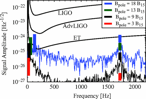
Figure 8: GW detectability of magnetar oscillations in giant flares. We show the signal amplitude $\sqrt{T}|h|$, where $h$ is the estimated dimensionless strain from magnetar oscillations in giant flares, and $T$ is the estimated damping time of the oscillation. The giant flare is modeled as the instability of the neutron star magnetic field (see text). The colored boxes on the left represent the $f$-mode signal, assuming $50$ ms$\leq T\leq 200$ ms. The colored boxes on the right represent the signal of a lower-frequency mode (Alfvén and/or $g$-modes), assuming $10$ ms$\leq T\leq 1$ s. Different colors correspond to different values of the magnetic field at the poles. We also show the signal for the entire spectrum, assuming a damping time $T=100$ ms (from Zink et al. (2012)).

Giant flares of magnetars are among the most luminous events in the universe. They are believed to be due to large-scale rearrangements of the magnetic fields, either in the stellar core Thompson and Duncan (1995, 2001) or in the magnetosphere Lyutikov (2006); Gill and Heyl (2010). Even a tiny part of their energy could excite non-radial oscillations of the neutron star - in particular, the $f$-mode - and thus be emitted through GWs. Preliminary estimates Corsi and Owen (2011) were very optimistic on the detectability of the $f$-mode excited by giant flares, but they were based on the assumption that the energy emitted in GWs by $f$-mode excitation is comparable to the total magnetic energy of the star. More accurate estimates Levin and van Hoven (2011) showed that only a small part of the magnetic energy is converted in GWs. Assuming that the released electromagnetic energy is of the order of the magnetic energy of the star, a giant flare at $D=10$ kpc would excite an $f$-mode GW signal detectable by Advanced LIGO/Virgo with a SNR Levin and van Hoven (2011)

$$\frac{S}{N}\lesssim 10^{-2}B_{15}^{2}\,,$$ (36)

where $B_{15}$ is the (normalized) magnetic field-strength at the poles. This result, based on a perturbative analysis, implies that the $f$-mode would definitely not be detectable by second-generation interferometers if $B\sim 10^{15}$ G, but it may be marginally detectable for $B\sim 10^{16}$ G.

Subsequently, giant flares and their coupling with the neutron star oscillations have been studied using general-relativistic MHD numerical simulations of the magnetic field instability in magnetars Ciolfi and Rezzolla (2012); Zink et al. (2012). This is a toy-model which mimics the catastrophic magnetic field rearrangments during a giant flare, and allows to estimate the amplitude and the features of the GW emission. The numerical simulations show a power-law relation between the emitted gravitational signal and the surface magnetic field-strength (in these models the magnetic field-strength at the surface and in the interior are comparable) Zink et al. (2012):

$$h\sim 7.6\times 10^{-27}\frac{B_{15}^{3.3}}{D_{1}}\,,$$ (37)

where $D_{1}$ is the distance of the source normalized to $1$ kpc. Most of the energy in the signal is in the $f$-mode, but also lower frequency modes (likely Alfvén and/or composition $g$-modes) are excited (see Fig. 8).

The results of numerical simulations Ciolfi and Rezzolla (2012); Zink et al. (2012) are even more pessimistic than those of perturbation theory Levin and van Hoven (2011) shown in Eq. (36). The SNR of the GW signal from an $f$-mode excitd by a giant flare has been estimated to be Ciolfi and Rezzolla (2012) $S/N\sim 10^{-4}B_{15}^{2}$ for Advanced LIGO/Virgo, and $S/N\sim 10^{-2}B_{15}^{2}$ for ET.

The numerical simulations of Zink et al. (2012) give similar results, see Fig. 8. The SNR can be read off the figure, as the ratio between the signal and the noise curve, for a given $B_{pole}$ and for a given detector. As mentioned above, Fig. 8 also shows a low-frequency mode, whose SNR is comparable (but sligthly larger) than that of the $f$-mode.

These studies confirm that the gravitational emission from mode excitation in magnetar flares can not be detected by advanced GW detectors. This signal is expected to be too weak to be detected even by third-generation GW experiments, such as ET, unless the surface magnetic field is $\gtrsim 10^{16}$ G Zink et al. (2012); Ciolfi and Rezzolla (2012), i.e. an order of magnitude larger than the observed magnetic fields.

VII Neutron star “mountains”

Rotating neutron stars symmetric with respect to the rotation axis do not emit gravitational radiation. However, if a neutron star is not perfectly axisymmetric it emits GWs, mostly at frequencies $f_{\rm spin}$ and $2f_{\rm spin}$ (where $f_{\rm spin}$ is the rotation frequency). Most of the observed neutron stars have rotation frequencies in the range between $\sim 10$ Hz and $1$ kHz, which is the range where ground-based interferometers such as Advanced LIGO/Virgo are most sensitive. Therefore, if the deviation from axisymmetry is large enough, rotating neutron stars can be promising sources of GWs.

The deviation from axisymmetry is described by the quadrupole ellipticity

$$\varepsilon=\frac{Q}{I}\,,$$ (38)

where $Q$ is the mass quadrupole moment associated to the distortion (i.e. excluding the contribution of rotation, which is necessarily axisymmetric and is not associated to GW emission), and $I$ is the moment of inertia of the rotation axis. Such distortions are called mountains. When $\varepsilon>0$ the star is oblate, while when $\varepsilon<0$ it is prolate.

If the distortion has a symmetry axis forming an angle $\alpha$ (called wobble angle) with the rotation axis, the amplitude of the GW emission is Zimmermann and Szedenits (1979); Bonazzola and Gourgoulhon (1996)

$$h_{0}\simeq\frac{4\pi^{2}G}{Dc^{4}}f_{\rm gw}^{2}I\varepsilon\sin\alpha\simeq 4\times 10^{-24}P_{-3}^{-2}\,D_{1}^{-1}I_{45}\left(\frac{\varepsilon}{10^{-6}}\right)\,.$$ (39)

The deformation can be due to different mechanisms: from the magnetic field of the star Bonazzola and Gourgoulhon (1996); Haskell et al. (2008); Ciolfi et al. (2010) (“magnetic mountains”), to temperature gradients in the crust leading to local deformation sustained by the elastic strain  Bildsten (1998b); Ushomirsky et al. (2000) (“thermal mountains”). The former can arise both in isolated neutron stars (magnetars, but also in “ordinary” neutron stars), or in accreting neutron stars. The latter, instead, can only be formed in accreting neutron stars, because the temperature gradients are created by asymmetries in the matter accreting by a companion object.

Current searches for GWs from rotating pulsars using first generation LIGO/Virgo have shown no sign of such emission (see e.g. Aasi et al. (2014) and references therein). However, this negative result allows us to place upper limits on the quadrupole ellipticity of the pulsars under study; in the case of the Crab pulsar, $\varepsilon\lesssim 8.6\times 10^{-4}$; in the case of other pulsars, the upper limits are significantly weaker. These limits are below the theoretical bounds (see below), but (in some cases) they exceed the spin-down limit on $\varepsilon$, which has been obtained with the unrealistic assumption that the observed pulsar spin-down is only due to GW emission.

In the following we shall first discuss current models of neutron stars deformed by a magnetic field, and then the different astrophyiscal scenarios for magnetic mountains. We shall then discuss thermal mountains, and other possible neutron star deformations in the context of neutron star models with exotic matter and/or pinned superfluidity.

VII.1 Modelling magnetic mountains

Chandrasekhar and Fermi Chandrasekhar and Fermi (1953) (see also Ferraro (1954)) first pointed out that magnetic fields induce quadrupolar deformations on spherically symmetric stars, with ellipticities (which we hereafter denote by $\varepsilon_{\rm B}$) of the order of the ratio between the magnetic energy $E_{\rm B}$ and the gravitational energy $E_{G}$, i.e.

$$\varepsilon_{\rm B}\sim\frac{E_{\rm B}}{E_{\rm G}}\sim\frac{R^{3}\langle B^{2}\rangle}{GM^{2}/R}\sim(10^{-6}-10^{-5})\langle B_{15}^{2}\rangle\,,$$ (40)

where $\langle B^{2}\rangle$ is the volume-averaged square field strength. It was later noted Wentzel (1960); Ostriker and Gunn (1969) that the magnetic-induced quadrupole ellipticity $\varepsilon_{\rm B}$ can be positive or negative, i.e. the shape of the star can be oblate or prolate, depending on the magnetic field structure. Indeed, neutron star magnetic fields can have poloidal or toroidal structure, and poloidal fields $B_{\rm pol}$ tend to deform the star to an oblate shape, while toroidal fields $B_{\rm tor}$ tend to deform it to a prolate shape. When poloidal and toroidal components are both present, the deformation has both positive and negative contributions. For instance, in a specific example of magnetic field geometry the deformation has been estimated to be Ostriker and Gunn (1969)

$$\varepsilon_{\rm B}\sim E_{G}^{-1}R^{3}\left(3\langle B^{2}_{\rm pol}\rangle-\langle B^{2}_{\rm tor}\rangle\right)\,.$$ (41)

The relative contributions of poloidal and toroidal components can change if the magnetic field geometry is different.

Similar estimates have been derived for a neutron star with a superconducting phase (see the discussion below), in the case of a purely toroidal field Cutler (2002):

$$\varepsilon_{\rm B}\sim 10^{-6}\langle B_{15}\rangle\frac{H_{\rm c1}}{10^{15}\,G}\,,$$ (42)

where $H_{\rm c1}$ (which is believed to be $\sim 10^{15}$ G in neutron star cores Glampedakis et al. (2011b)) is the critical field strength characterizing superconductivity. These expressions have been computed for a constant density star, and assuming a dipole field configuration. However, as we discuss below, more sophisticated numerical analyses show that Eqns. (40), (41), (42) give good order-of-magnitude estimates for magnetic deformations of neutron stars.

When a neutron star is prolate (which requires a prevailing toroidal field), a spin-flip mechanism can take place Jones (1975); Cutler (2002), in which the wobble angle grows until the symmetry axis and the rotation axis become orthogonal: an optimal geometry for GW emission (see Eq. (39)).

Presently, we do not have direct information on the internal structure of neutron star’s magnetic fields. However, it is generally believed that they should have both a poloidal and a toroidal component. Indeed, analytical computations Prendergast (1956); Tayler (1973) and numerical simulations Braithwaite (2006, 2007) show that purely poloidal and purely toroidal configuration are unstable in an Alfvén timescale. Conversely, poloidal-toroidal magnetic fields can develop from the evolution of arbitrary initial fields Braithwaite and Spruit (2004). The fields found in Braithwaite and Spruit (2004); Braithwaite and Nordlund (2006) have a so-called “twisted-torus” structure: a poloidal magnetic field extending throughout the star and in the exterior, and a toroidal field confined to a torus-shaped region inside the star.

GR and Newtonian models of stationary neutron star configurations with a twisted-torus magnetic field have been carried out in Ciolfi et al. (2010); Lander and Jones (2009). They are based on the numerical integration of the GR MHD equations for an axisymmetric ideal fluid (which can be reduced to a single partial differential equation, the so-called Grad-Shafranov (GS) equation), and predict that the magnetic field induces a quadrupole ellipticity $\sim(10^{-6}-10^{-5})~{}B_{15}^{2}$ (where $B_{15}$ is the surface magnetic field) , consistent with the estimates (40), (41). Moreover, the results of Ciolfi et al. (2010); Lander and Jones (2009) show that in a twisted-torus configuration, the ratio of toroidal field energy over poloidal field energy is $\langle B_{\rm tor}^{2}\rangle/\langle B_{\rm pol}^{2}\rangle\lesssim 0.15$. Therefore, in these configurations the poloidal field prevails, the star is oblate, and the spin-flip mechanism does not occur. More recently, twisted-torus configurations (with $\langle B_{\rm tor}^{2}\rangle/\langle B_{\rm pol}^{2}\rangle\lesssim 0.1$) have also been described by solving the fully non-linear Einstein-Maxwell’s equations, see e.g. Pili et al. (2014); Uryu et al. (2014).

A different class of twisted-torus configurations has later been found in Ciolfi and Rezzolla (2013), where - with an appropriate prescription of the azimuthal currents - the ratio $\langle B_{\rm tor}^{2}\rangle/\langle B_{\rm pol}^{2}\rangle$ can be as large as $\sim 0.9$, i.e. the toroidal field can prevail. In these models the deformation of the star is larger than the prediction of Eqns. (40), (41) by a factor $\sim 100$

$$\varepsilon_{\rm B}\sim 10^{-4}B_{15}^{2}\,.$$ (43)

The equilibrium properties of the magnetized star depend on whether the EOS is barotropic or non-barotropic. The models in Ciolfi et al. (2010); Lander and Jones (2009); Ciolfi and Rezzolla (2013) assume a barotropic EOS. As shown in Mastrano et al. (2011); Glampedakis and Lasky (2016), if the EOS is non-barotropic one is free to prescribe the magnetic field, and the ratio between toroidal and poloidal energy becomes a free parameter, even though it is likely to be constrained by the requirement of stability. In the model studied in Mastrano et al. (2011),

$$\varepsilon_{\rm B}\sim 10^{-5}B_{15}^{2}\left(1-0.64\frac{\langle B_{\rm tor}^{2}\rangle}{\langle B_{\rm pol}^{2}\rangle}\right)\,.$$ (44)

If the ratio $\langle B_{\rm tor}^{2}\rangle/\langle B_{\rm pol}^{2}\rangle$ is sufficiently large, i.e. the toroidal field prevails, the deformation can be as large as that described by Eq. (43). In these configurations (such as in those studied in Ciolfi and Rezzolla (2013)) the neutron star is prolate, and the spin-flip mechanism can take place.

If higher-order multipoles of the magnetic field are present, the (prolate) deformation can be even larger Mastrano et al. (2015). Alternative geometries with poloidal-toroidal fields have also been studied, such as the “tilted torus” configuration, in which the poloidal and the toroidal fields have misaligned symmetry axes Lasky and Melatos (2013).

The models discussed above do not take into account the fact that outer cores of neutron star are expected to contain superconducting protons (and superfluid neutrons). In a (type II) superconducting phase, the magnetic field is quantized into fluxtubes surrounded by non-magnetised matter. The force exerted by the quantized field is not the Lorentz force, but a fluxtube tension force Mendell (1991); Glampedakis et al. (2011b); therefore, the description based on the GS equation is not adequate to model the superconducting phase (even though they still obey a GS-type equation). In recent years, the deformation of magnetized superconducting neutron stars has been computed by numerical integrations of the equations for the fluxtube magnetic force for toroidal fields Akgun and Wasserman (2008); Lander et al. (2012), for purely poloidal fields Henriksson and Wasserman (2013), and for twisted-torus fields Lander (2013). All these computations give deformations consistent with the analytical estimates Cutler (2002) of Eq. (42).

We remark that $\varepsilon_{\rm B}\sim B^{2}$ in non-superconducting neutron stars, while $\varepsilon_{\rm B}\sim B$ in neutron stars with a superconducting phase. This is due to the different magnetic force acting in superconducting matter. Comparing Eqns. (40), (43), we can see that in magnetars (with $B\sim 10^{15}$ G) the magnetic deformations have the same order of magnitude regardless of whether a superconducting phase is present; conversely, in ordinary neutron stars - such as the observed pulsars - the magnetic field strength is $\sim 10^{12}$ G or smaller, and magnetic deformations are much larger if a (type II) superconducting phase is present.

VII.2 Magnetic mountains in newly-born magnetars and in known pulsars

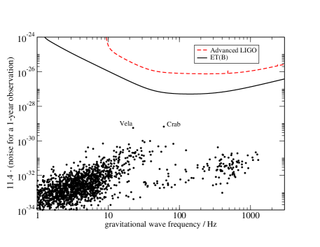
Figure 9: GW detectability of magnetic mountains in known pulsars. GW strain from the population of known pulsars, assuming a $1$-year phase coherent observation and quadrupole deformations given by Eq. (42). The detector noise curves were taken from LIG ; ETc . All pulsar data were taken from the ATNF database ATN .

As we discussed in Sec. VI, observations of SGRs and AXPs, with their large spin-down rates and intense burst activity, suggest that these objects are magnetars Duncan and Thompson (1992). Due to their very large magnetic fields, magnetars are expected to have the largest magnetic mountains. However, since the observed SGRs and AXPs have low spin frequencies, they cannot be GW sources for ground-based interferometers.

The standard magnetar model Duncan and Thompson (1992); Goldreich and Reisenegger (1992) predicts that the strong magnetic fields form at the birth of the neutron star, through convection and dynamo effects, and can last for $\sim 10^{4}-10^{5}$ years Goldreich and Reisenegger (1992); Pons and Geppert (2007). If this scenario is accurate, a non-negligible fraction ($\sim 10\%$) of newly-formed neutron stars can be born as magnetars Kouveliotou et al. (1998); Woods and Thompson (2006), and, if their rotation rates are large enough, they can be potential sources for GW detectors (see e.g. Dall’Osso et al. (2009)). Presently, it is not clear what the actual rotation rate of newly-born neutron stars is; current estimates suggest that it should not be larger than few hundreds of Hz (see e.g. Camelio et al. (2016) and references therein). A newly-born magnetar with $B\sim 10^{15}$ G could have a quadrupole deformation $\varepsilon_{\rm B}\sim 10^{-6}-10^{-5}$ (40) (even larger if the toroidal field prevails, see Eq. (43)). If $D\sim 10$ kpc and $P\sim 10$ ms, it may yield a GW strain (39) $h_{0}\sim 10^{-26}$ , potentially detectable by ET. However, the event rate of galactic newly-born magnetars (comparable with that of galactic supernovae) is too low to make them a promising GW source.

We have observed, instead, several pulsars with magnetic field-strengths $\lesssim 10^{12}$ G, and rotation rates in the bandwidth of ground-based GW detectors. The GW emission from these objects is negligible, unless a type II superconducting phase is present. Indeed, when $B\sim 10^{12}$ the estimate for (type II) superconducting stars (42) is $\varepsilon_{\rm B}\sim 10^{-9}$, while the estimate for non-superconducting stars (40) is a factor $\sim 1000$ smaller. As noted in Andersson et al. (2011), a (superconducting) MSP with $B\sim 10^{12}$ G at $D=1$ kpc would then emit a GW strain $h_{0}\sim 10^{-27}$, marginally detectable by ET. This estimate, however, is probably too optimistic: all known MSPs have magnetic fields much smaller than $10^{12}$ G, while pulsars with $B\sim 10^{12}$ have periods much larger than $\sim 1$ ms. In Fig. 9 we show the GW strain for the population of known pulsars, assuming that the quadrupole deformation is given by the estimate (42), corresponding to the presence of a type-II superconducting phase in the core. We can see that, under these assumptions, the expected signal from known pulsars would be well below the sensitivity curves of second- and third-generation interferometers.

VII.3 Magnetic mountains in millisecond magnetars from compact binary mergers

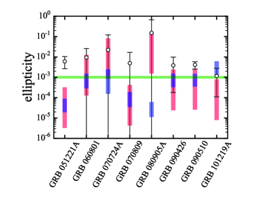
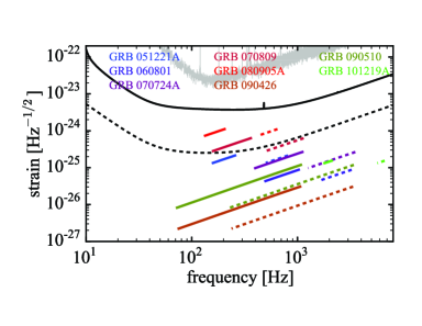
Figure 10: Observational upper limits on magnetar deformation and GW emission. Left panel: Upper limits on the neutron star ellipticity from eight short GRBs, given by Eq. (45) (black point with error bars). The red bars show the theoretical estimate from Eq. (40). The blue bars show the range of maximal ellipticities for which the spin flip can take place. The green line represents the ellipticity which can be induced by $f$-mode excitation (see section IV). Right panel: Upper limits on the GW strain amplitude evolution, compared with the sensitivity curves of Advanced LIGO and ET, for $\eta=0.1$ (dotted lines) and for $\eta=1$ (solid lines). The observation time is assumed to be $10^{5}$ s for GRBs with power-law decay, while it coincides with the GRB emission time for those with steeper decay (figure from Lasky and Glampedakis (2016)).

Binary neutron star mergers can result in strongly magnetized neutron stars Zhang (2013); Giacomazzo and Perna (2013). They can be meta-stable supramassive neutron stars living from few seconds to hours Ravi and Lasky (2014), but can also be stable neutron stars Giacomazzo and Perna (2013). These objects have been proposed to be the central engine of short GRB, in the so-called millisecond magnetar model Dai and Lu (1998); Zhang and Mészáros (2001); Rowlinson et al. (2013). In this scenario, the energy injection in the GRB is due to dipole radiation from a spinning-down magnetar. Strong evidence supporting the millisecond magnetar model is its ability to explain the shape of the observed GRB X-ray spectra, which are characterized by a plateau of $\sim 10-10^{2}$ s followed, in most cases, by a power-law decay; in a subset of short GRBs, instead, the decay is much steeper. The X-ray spectrum from a spinning-down magnetar resulting from a compact binary coalescence would have the same structure: a plateau followed by a power-law decay if the neutron star is stable, by a steeper decay if it is a supramassive star eventually collapsing to a black hole.

The millisecond magnetar model is probably the most promising astrophysical scenario for GW detection from magnetic mountains. Indeed, numerical simulations show that the magnetars resulting from a binary neutron star coalescence would have periods of the order of milliseconds - significantly smaller than the expected periods of newly-born neutron stars. Moreover, in this scenario we have astrophysical data from these objects, since they would be the engine of short GRBs.

Preliminary estimates Dall’Osso et al. (2015) show that the GW emission from these sources could be marginally detectable by second-generation interferometers, and detectable by third-generation interferometers such as ET (even more optimistic estimates have been derived in Corsi and Meszaros (2009)). However, these computations are based on the assumption that GW emission gives a significant contribution to the magnetar spin-down. Since the millisecond magnetars predicted in this model are progenitors of short GRBs, the assumptions of the model can be tested against GRB observations.

In Lasky and Glampedakis (2016), observations of the X-ray light curve of short GRBs have been used to constrain the ellipticity of the (stable) neutron stars produced in the merger, and then to set a bound on the GW emission from these objects. Indeed, the late time tail of the observed X-ray spectrum is $\sim t^{-2}$, suggesting that the spin-down is mainly due to dipole electromagnetic emission rather than to GW emission. Therefore, the comparison between the observed X-ray spectrum and the predictions of the model allows to set an observational upper limit on the neutron star ellipticities:

$$\varepsilon_{\rm B}\lesssim 0.33\,\eta\,I_{45}^{1/2}\,\left(\frac{L_{\rm em}}{10^{49}\,{\rm erg/s}}\right)^{-1}\,\left(\frac{t_{\rm b}}{100\,{\rm s}}\right)^{-3/2}\,,$$ (45)

where $\eta\leq 1$ is the conversion efficiency of spin-down energy into X-ray luminosity, $L_{{\rm em}}$ is the short GRB luminosity in the inital plaeau phase, and $t_{\rm b}$ is the plateau duration. This upper limit (through Eq. (39)) corresponds to an upper limit on the expected GW signal. The analysis of Lasky and Glampedakis (2016) shows that the agreement between the observed X-ray spectrum and the predictions of the model requires that the magnetar spin-down is mainly due to dipole emission, with a very small contribution from GW emission. Therefore, these signals are not expected to be detected by Advanced LIGO/Virgo, but are potentially detectable by third-generation interferometers such as ET. This can be seen in Fig. 10. In the left panel we show the upper limit (45) on the neutron star ellipticities, assuming $\eta=0.1$ (black points with error bars) for eight observed short GRBs. In the right panel we show the corresponding upper limits on the GW strain amplitude evolution, for $\eta=0.1$ (dotted lines) and for $\eta=1$ (solid lines), compared with the sensitivity curves of Advanced LIGO and ET.

VII.4 Magnetic mountains in accreting systems

Magnetic mountains can also form in LMXBs. In this case, the mountain - a localized deformation - is formed by the accreting matter, but it is sustained by the magnetic field. Since the mountain is not sustained by crustal rigidity, its quadrupole ellipticity can be larger than the upper bound associated to the maximum crustal strain Ushomirsky et al. (2000). In this scenario Payne and Melatos (2004); Melatos and Payne (2005); Vigelius and Melatos (2008), accreted matter accumulates in a column over the polar cap, distorting the magnetic field and reducing the magnetic moment of the star. As the stars accretes, the exterior magnetic field evolves approximately as $B=B_{*}(1+M_{\rm acc}/M_{\rm c})^{-1}$ where $B_{*}$ the field when accretion starts, $M_{\rm acc}$ the accreted matter and $M_{\rm c}$ the critical accreted mass above which the magnetic moment starts to change Shibazaki et al. (1989). The quadrupole ellipticity associated to magnetic mountains in LMXB is Priymak et al. (2011); Haskell et al. (2015)

$$\varepsilon\sim\frac{M_{\rm acc}}{M_{\odot}}\left(1+\frac{M_{\rm acc}}{M_{\rm c}}\right)^{-1}\,,$$ (46)

where $M_{\rm c}\sim 10^{-7}(B_{*}/10^{12}G)^{4/3}$. This formula is only accurate for $M_{\rm acc}\lesssim M_{\rm c}$: for larger values of the accreted mass, the quadrupole ellipticity saturates. Dynamical MHD simulations suggest that these deformations can persist for timescales of the order of $\sim 10^{5}-10^{8}$ years Vigelius and Melatos (2009).

Although magnetic fields of LMXBs are much weaker than those of magnetars, the quadrupole ellipticities of local mountains can be much larger than those produced by a global magnetic deformation of the star. Moreover, LMXBs have rotation rates much larger than those of magnetars, well within the sensitivity band of ground-based interferometers. Fast rotation also enhances the GW signal from a deformed star. Therefore, as shown in Priymak et al. (2011); Haskell et al. (2015), a buried field $B_{*}\gtrsim 10^{12}$ G could generate a deformation, and then a GW emission, strong enough to be detected by Advanced LIGO/Virgo Priymak et al. (2011); Haskell et al. (2015).

VII.5 Thermal mountains

Accreting neutron stars in LMXBs can have quadrupolar deformations due to temperature gradients in the accreted crust Bildsten (1998b); Ushomirsky et al. (2000). Indeed, as the matter accretes, it is buried and compressed until nuclear reactions occur (electron capture, neutron emission, etc.) Haensel and Zdunik (1990). These reactions heat the crust, and since the accreted matter is expected to be asymmetric, the temperature gradient produced by nuclear reactions is also asymmetric, giving rise to quadrupolar deformations in the neutron star. These deformations are called “thermal mountains”; they also belong to the broader class of “elastic mountains”, i.e. deformations sustained by the elastic strain of the crust. Presently, thermal gradients are the only known viable mechanism to produce elastic mountains.

The deformation due to a thermal gradient with quadrupolar component $\delta T_{\rm q}$ (which we denote by $\varepsilon_{\rm th}$) is Ushomirsky et al. (2000); Haskell et al. (2015)

$$\varepsilon_{\rm th}\sim 10^{-10}R_{6}^{4}\left(\frac{\delta T_{\rm q}}{10^{5}\,{\rm K}}\right)\left(\frac{Q}{30\,{\rm MeV}}\right)^{3}\,,$$ (47)

where $Q$ is the threshold energy of electron capture by nuclei. The quadrupolar thermal gradient is just a fraction of the total thermal gradient $\delta T$, which is expected to be, at most, of the order of $10^{6}$ K Ushomirsky and Rutledge (2001), if produced by an outburst. In the most optimistic scenario $\delta T_{\rm q}\lesssim 0.1\,\delta T\lesssim 10^{5}$ K , yielding a thermal mountain of the order of $\varepsilon_{\rm th}\sim 10^{-10}$ Haskell et al. (2015). The GW strain (39) from this deformation would be $h_{0}\sim 10^{-27}-10^{-28}$, too weak to be detected by Advanced LIGO/Virgo, but potentially detectable by third-generation GW intereferometers such as ET. This can be seen in Fig. 11, where we show the estimated GW strain from a set of observed LMXBs, computed from Eqns. (47) and (39), for different values of the electron capture threshold energy $Q$ and assuming $\delta T_{\rm q}\simeq 10^{5}$ K. In the figure, the Advanced LIGO and ET sensitivity curves are shown for different values of the integration time (one month, which is a typical outburst duration, and two years) because the persistence timescale of the mountain, and then the typical duration of the signal, is presently poorly constrained. In the most favourable case (the deformation persists after the outburst, $\delta T_{\rm q}/\delta T\simeq 0.1$) some of the systems could emit a signal detectable by ET. We note, however, that this value of $\delta T_{\rm q}/\delta T$ is an upper limit with no solid physical motivation; if the actual value of this ratio is smaller than $\sim 0.1$, even third-generation GW interferometers will not be able to detect thermal mountains.

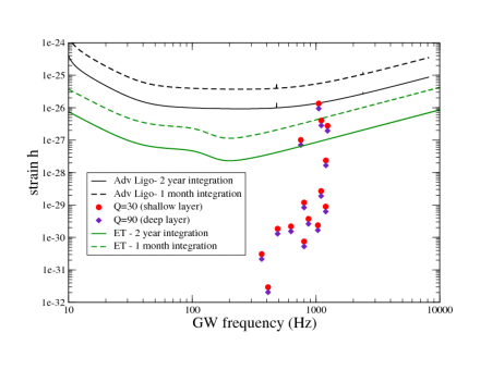
Figure 11: Detectability of thermal mountains. We show the estimated GW strain from thermal mountains formed in a set of observed LMXB outbursts, for different values of the reaction threshold energy $Q$, assuming $\delta T_{\rm q}\simeq 10^{5}$ K. The detector noise curves assume one month (dashed) or two years (solid) of phase-coherent observation (from Haskell et al. (2015)).

The GW emission from thermal mountains, regardless of its direct detectability, may have a role in the spin evolution of LMXBs. Twenty years ago, thermal mountains have been proposed to explain the apparent spin cut-off in LMXBs Bildsten (1998a). However (as discussed in detail in Sec. V.1), it was later understood that this feature can probably be explained in terms of the coupling of the stellar magnetic field with the accretion disk. More recently, thermal mountains have been revived by the observations of the pulsar PSR J$1023+0038$, which shows a transition between a radio MSP state and a LMXB state Archibald et al. (2009). Remarkably, the pulsar spins down faster (by $\sim 20\%$) during the LMXB state. It has been suggested Haskell and Patruno (2017) that this enhanced spin-down is due to GW emission by a thermal mountain. To explain the additional spin-down, a deformation $\varepsilon_{\rm th}\sim 5\times 10^{-10}$ would be required, which - as we have discussed above - can indeed be a thermal mountain, and would emit gravitational radiation detectable by third-generation interferometers such as ET. If these results are confirmed, they will provide the first observational indirect evidence supporting the existence of GW emission from neutron star mountains.

Thermal mountains (and more generally, elastic mountains) are limited by the maximum stress that the crust can sustain before breaking Ushomirsky et al. (2000); Haskell et al. (2006); Johnson-McDaniel and Owen (2013):

$$\varepsilon_{\rm th}\lesssim\frac{\mu_{\rm cr}\sigma_{\rm br}V_{\rm cr}}{GM^{2}/R}\sim 10^{-5}\left(\frac{\sigma_{\rm br}}{0.1}\right)\,,$$ (48)

where $\mu_{\rm cr}$ is the shear modulus of the crust, $V_{\rm cr}$ is the volume of the crust, and $\sigma_{\rm br}$ is the crustal breaking strain, which could be as large as $\sim 0.1$ Horowitz and Kadau (2009) .

We remark that this is just an upper bound: there is no reason to believe that neutron star have deformations close to this value. For instance, the thermal mountain which has been suggested in Haskell and Patruno (2017) to explain the observations of PSR J$1023+0038$ is much smaller than the deformation in Eq. (48). We also remark that this bound applies to thermal mountains (more generally, to elastic mountains), but it does not necessarily apply to magnetic mountains. Indeed, when the crust forms in a newly-born neutron star the magnetic deformation may already be present; in this case, the equilibrium shape of the crust would be non-spherical, and the crust would not have to sustain an elastic strain, at least while the magnetic field is present.

VII.6 Exotic mountains

The ellipticities associated with the neutron star deformations discussed so far are clearly pessimistic from the perspective of GW observability. A somewhat more promising situation may arise if we consider neutron stars with quark matter cores. If present, quarks are most likely to find themselves in a color-superconducting state, the exotic properties of which could accommodate significantly larger quadrupolar deformations (of both magnetic and elastic nature) as compared to conventional hadronic matter.

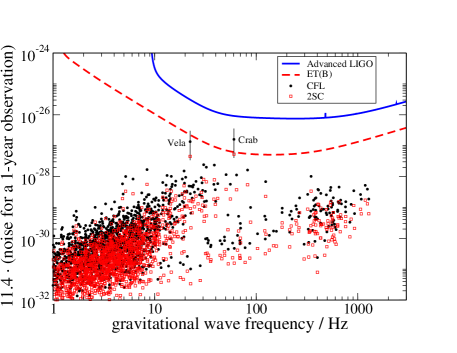
Figure 12: GW detectability of color-magnetic mountains. In this figure, adapted from Glampedakis et al. (2012), we show the estimated GW strain (assuming a 1-year phase-coherent observation) from the population of known pulsars, assuming they have CFL (or 2SC) quark cores. We have used the fiducial parameters $\mu_{q}=400\,\mbox{MeV}$, $V_{q}=0.5V_{\rm star}$, and $\langle B\rangle=2B_{\rm surf}$.

Among the various possible quark matter incarnations (for a review see Alford et al. (2008)) the color-flavor-locked (CFL) phase, where all three quark species $(u,d,s)$ are paired, appears to be the most favoured one. Another well-studied phase is the two-flavor superconducting (2SC) state where just the $(u,d)$ quarks pair. Both of these phases come with remarkable magnetic permeability properties. The stellar magnetic field threading a CFL/2SC core is likely to do so by forming an array of quantised vortices in the same way that fluxtubes are formed in the more familiar type II protonic superconductor Iida and Baym (2002); Alford and Sedrakian (2010). These vortices, however, are color-magnetic (rather than just magnetic) in the sense that they are carriers of an admixture of magnetic and gluonic field degrees of freedom. The latter component is the dominant one and, as a consequence, the energy per unit length ${\cal E}_{\rm X}$ (where X labels the phase) of a color-magnetic vortex can be 2-3 orders of magnitude higher than that of a conventional protonic fluxtube Iida and Baym (2002); Alford and Sedrakian (2010). This property entails an amplified vortex array tension and opens the possibility of creating a large deformation in a neutron star’s CFL/2SC core Glampedakis et al. (2012). The ellipticity of this internal color-magnetic mountain can be estimated by means of the ratio of the vortex array tension energy to the stellar gravitational energy:

$$\varepsilon_{\rm X}\approx\frac{{\cal N}_{\rm X}{\cal E}_{\rm X}V_{q}}{GM^{2}/R},$$ (49)

where ${\cal N}_{\rm X}$ is the vortex surface density and $V_{q}$ is the volume of the quark core. For a CFL core (and assuming canonical stellar parameters) this expression leads to Glampedakis et al. (2012),

$$\varepsilon_{\rm cfl}\approx 10^{-7}\langle B_{12}\rangle\left(\frac{V_{q}}{V_{\rm star}}\right)\left(\frac{\mu_{q}}{400\,\mbox{MeV}}\right)^{2},$$ (50)

where $\mu_{q}$ is the strange quark chemical potential (normalised to a canonical value) and, as before, $\langle B\rangle$ represents the volume-averaged interior magnetic field.

The GW strain associated with this deformation can be estimated with the help of Eq. (39), using reasonable values for the various parameters, i.e. $\mu_{q}=400\,\mbox{MeV}$, $V_{q}=0.5V_{\rm star}$ and $\langle B\rangle=2B_{\rm surf}$ (as suggested by models of MHD equilibria in neutron stars, see e.g. Ciolfi et al. (2009); Lander and Jones (2009)). The resulting GW detectability by Advanced LIGO and ET of the pulsar population with known surface dipole fields $B_{\rm surf}$ is shown in Fig. 12. When compared to Fig. 9, it is evident that the presence of a color-magnetic deformation in neutron stars leads to a marked improvement in the strength of their GW signature. The results presented here suggest that young pulsars such as the Crab or the Vela could be detectable by ET. A much larger fraction of the pulsar population could become detectable (even by Advanced LIGO/Virgo) if we assume a higher magnetic field ratio $\langle B\rangle/B_{\rm surf}$.

A drastically different phase of quark matter could be that of a crystalline color-superconductor (CCS) Rajagopal and Sharma (2006); Mannarelli et al. (2007), effectively leading to a neutron star with a solid core. Given that the shear modulus $\mu_{\rm ccs}$ of CCS matter is estimated to be much higher than that of the crustal bcc lattice Mannarelli et al. (2007), the elastic deformation that could be sustained by a solid quark core could be significantly greater than that of normal hadronic neutron stars. For obtaining the ellipticity of the CCS mountain we can use a formula similar to Eq. (40). We find,

$$\varepsilon_{\rm ccs}\approx\frac{\mu_{\rm ccs}V_{q}\sigma_{\rm br}}{GM^{2}/R}\approx 6\times 10^{-4}\left(\frac{V_{q}}{V_{\rm star}}\right)\left(\frac{\mu_{q}}{400\,\mbox{MeV}}\right)^{2}\left(\frac{\Delta_{q}}{10\,\mbox{MeV}}\right)^{2}\left(\frac{\sigma_{\rm br}}{0.01}\right),$$ (51)

where $\Delta_{q}$ is a quark gap parameter (normalised to a canonical value) and the (highly uncertain) breaking strain of a crystalline quark core is normalized to the fiducial value $\sigma_{\rm br}\sim 0.01$. This simple estimate is in good agreement with the results of more rigorous calculations Owen (2005); B. Haskell, N. Andersson, D. I. Jones and L. Samuelsson (2007) and is about a factor $\mu_{\rm ccs}/\mu_{\rm cr}\sim 10^{3}$ higher than the maximum elastic deformation of the crust (Eq. (48)). As discussed in B. Haskell, N. Andersson, D. I. Jones and L. Samuelsson (2007), the presence of such a large internal deformation in neutron cores could in principle be tested by the upper limits set by GW searches. According to the recently published Advanced LIGO results Abbott et al. (2017e) the most stringent upper limit is $\varepsilon\approx 10^{-7}$ which is well below the result (51). However, the non-detection of GWs can only be used as a constraint for the (unidentified) non-axisymmetric straining mechanism or the poorly known $\sigma_{\rm br}$ and not as evidence against the existence of CCS matter.

From our brief exposition of deformations related to the presence of quark matter in neutron star cores it should have become clear that observation of GWs from such sources could provide strong evidence in favour of the existence of these very exotic states of matter. But it should also be remembered that the properties of quark matter in neutron stars are largely uncertain and therefore any theoretical predictions based on them should be viewed in a similar way.

VII.7 Mountains and pinned superfluidity

The presence of a pinned neutron superfluid component in the interior of neutron stars may lead to glitches (see next section) but could also have a number of interesting implications related to mountains. Vortex pinning could take place in the crust (with the pinning sites provided by the crustal lattice) and/or in the fluid core as a result of the interaction of the neutron vortices with the fluxtubes of the proton superconductor.

As discussed in Jones (2010), an elastically or magnetically deformed neutron star with a pinned superfluid component that has its angular momentum axis slightly misaligned with the stellar symmetry axes can modify the harmonic structure of the emitted GW signal by allowing emission at both frequencies $2\Omega$ and $\Omega$ (whereas only the former should be present in the absence of pinning and assuming a non-precessing state).

Incidentally, it is worth mentioning that the same pinned superfluid acts as a fixed gyroscope and could easily stabilise the previously discussed spin-flip instability of a strong toroidal magnetic field component Glampedakis and Jones (2010).

Finally, a pinned superfluid could itself act as a source of deformation and lead to GW mountain emission Jones (2002). Since this “Magnus mountain” is the only deformation mechanism that has not been considered so far in detail it is worth discussing it a bit more. As the name suggests, the straining mechanism responsible for this mountain is the Magnus force acting on the pinned superfluid vortices due to the spin lag between the superfluid and the normal stellar component onto which the vortices are attached (see Ruderman (1991a, b) for a more detailed discussion). Assuming both spin angular frequencies $\mathbf{\Omega}_{\rm n},\mathbf{\Omega}$ to be aligned along the same axis (say the $z$-axis) the resulting Magnus force is purely radial in cylindrical coordinates and has a per unit volume magnitude,

$$f_{\rm m}=2\varpi\rho_{n}\Omega_{\rm lag}\Omega,$$ (52)

where $\Omega_{\rm lag}=\Omega_{\rm n}-\Omega$ is the spin lag and $\varpi$ is the standard cylindrical radius. In order to produce a non-axisymmetric quadrupolar deformation, the force (52) itself has to have a similar non-axisymmetry. In turn, this requires a non-uniform distribution of pinned vortices which would entail a non-rigid body rotational profile for the superfluid. Although detailed calculations for this non-axisymmetric Magnus force are still lacking it is not too difficult to see how this property could come about in a realistic neutron star model. For example, if pinning is provided by the magnetic fluxtubes then the generic non-axisymmetry of the stellar magnetic field would imply a similar property for the spatial distribution of the pinning sites. In our present back-of the-envelope-analysis the non-axisymmetric character of the Magnus force can be accounted for by multiplication of (52) with a phenomenological dimensionless factor $\lambda\lesssim 1$.

The ellipticity of the resulting Magnus mountain can be estimated by means of the ratio between the volume-integrated Magnus force $F_{\rm m}=\int dVf_{\rm m}$ and the gravitational binding force Jones (2002):

$$\varepsilon_{\rm m}\sim\frac{F_{\rm m}}{F_{\rm grav}}\sim\frac{2\lambda\Omega_{\rm lag}\Omega R^{3}\rho V_{\rm pin}}{GM^{2}}\sim\frac{2\lambda\Omega_{\rm lag}\Omega R^{3}M_{\rm pin}}{GM^{2}},$$ (53)

where $V_{\rm pin}$ and $M_{\rm pin}$ represent the volume and mass of the pinned superfluid. Parametrising this result and assuming canonical stellar parameters we find,

$$\varepsilon_{\rm m}\sim 5\times 10^{-7}\lambda P_{-3}^{-1}\left(\frac{\Omega_{\rm lag}}{0.01\,\mbox{Hz}}\right)\left(\frac{M_{\rm pin}}{M_{\odot}}\right).$$ (54)

For the spin-lag we have used a representative value so that the Magnus force is at most comparable to the pinning force in the crust or in the core, see Link and Cutler (2002); Link (2003). Assuming $\lambda\sim 1$, we can see that a reasonable range for ellipticity could be $\varepsilon_{\rm m}\sim 10^{-7}-10^{-10}$, with the most favourable case coming from the scenario of vortex pinning in the core ($M_{\rm pin}\sim M_{\odot}$). As also concluded in Jones (2002), the expected Magnus mountain could be comparable to that due to magnetic or elastic stresses and therefore could be of interest.

VII.8 Future directions

In recent years our understanding of the different processes which can lead to neutron star mountains greatly improved. However, we still do not know which mountains are actually present in the different kinds of neutron stars (magnetars, radio pulsars, LMXB, etc.). Indeed, past and present astrophysical observations mainly probe the surface and the exterior of the star, while we have very limited information from its interior.

For instance, spin-down measurements give us accurate estimates of the exterior magnetic field of magnetars (and of ordinary neutron stars), but if the field inside the star is much larger than in the exterior, we will need know the interior field to find the size and shape of magnetic mountains. Theoretical modelling can be improved, for instance to better understand the stability properties of magnetic field configurations (which can tell us how much of the field is toroidal and how much is poloidal). MHD calculations of neutron stars with exotic matter would also be very important, because these objects can accomodate larger deformations than stars with conventional hadronic matter; as discussed above, existing calculations of these systems are only back-of-the-envelope estimates. In any case, we need observational data to know the actual (volume averaged) strength of the interior magnetic fields.

The same holds for thermal mountains. Theoretical modelling can clarify the mechanism leading to temperature anisotropies and can give us estimates of their actual shape and magnitude. In particular, we need to know the size of quadrupole contribution to temperature anisotropies, $\delta T_{\rm q}$. For instance, numerical simulations of the post-burst thermal evolution would help us understanding how large these mountains can be. However, even for thermal mountains, the power of theoretical modelling alone is limited: only observational data can tell us definitely how large actual mountains are.

The most promising observational probe to study neutron star mountains is the GW signal they emit as the star rotates. Once observed, this signal would provide a direct measurement of the mountain, shedding light on the formation mechanisms. Even an indirect GW observation, i.e., the observation in the electromagnetic spectrum of a process due to GW emission (such as the spin-down increase discussed in Haskell and Patruno (2017)) would give us valuable information to understand magnetic and thermal mountains and their formation.

VIII Glitches

Radio pulsars have extremely stable rotation rates - they are the most precise natural clocks in the universe - but some of them exhibit sudden increases in the rotation rate, called glitches. After the first glitch observations in the Vela and Crab pulsars Radhakrishnan and Manchester (1969); Reichley and Downs (1969); Boynton et al. (1969); Richards et al. (1969), more than three hundred glitches have been observed in $\sim 100$ pulsars Espinoza et al. (2011). More recently, glitches have also been observed in gamma-ray pulsars Ray et al. (2011); Pletsch et al. (2012) and in magnetars Dib et al. (2008) (MSPs can also have small glitches, but they are very rare Cognard and Backer (2004)).

The glitch occurs in a very short timescale, still unresolved by observations (the best upper limit is $\sim 40$ s Dodson et al. (2002)). The relative increase in the rotation rate $\Delta\Omega/\Omega$ ranges from $\sim 10^{-11}$ to $\sim 10^{-5}$ Espinoza et al. (2011), and is generally followed by an increase in the spin-down rate. Most glitches have $\Delta\Omega/\Omega\lesssim 10^{-7}$, but few of them (such as those of the Vela pulsar) are significantly larger, with $\Delta\Omega/\Omega>10^{-6}$.

The standard model of glitches is the superfluid model, in which glitches are due to superfluid neutrons in the neutron star interior, which store the angular momentum in a quantized array of vortices. The star spins down but its superfluid component does not, because the vortices are “pinned”, i.e. their positions are fixed. Periodically, some of the vortices “unpin”, move outwards and in this way the superfluid component removes the excess angular momentum, which is released in glitches.

An alternative model is the starquake model, in which glitches are due to the rigidity of the crust, which maintains its shape as the star spins down and reduces its quadrupole deformation; the strain on the crust increases and, periodically, there is a starquake, with a rearrangement of the moment of inertia and a glitch. This model can not explain large Vela-like glitches, but it is in principle possible that some small glitches are due to this mechanism. For a detailed discussion of the different glitch models, we refer the reader to Haskell and Melatos (2015) and references therein.

When a glitch occurs, there is a sudden rearrangement of the neutron star structure (in both the superfluid and the starquake models); therefore, glitches are expected to emit GWs. In 2006, during the fifth Science Run of LIGO, the Vela pulsar underwent a glitch. An analysis of the first-generation LIGO data looking for the excitation of stellar oscillations did not find a GW signal, thus setting an upper limit on the GW strain $h\leq 1.4\times 10^{-20}$ Abadie et al. (2011). However, second-generation detectors are expected to be about one order of magnitude more sensitive to this kind of signal.

Different mechanisms have been suggested for GW emission by pulsar glitches. They belong to two classes: the signals emitted during the glitch itself and those emitted during post-glitch relaxation.

• The energy released during the glitch can excite stellar oscillations Sidery et al. (2010); Keer and Jones (2015) (see also Sedrakian et al. (2003); Glampedakis and Andersson (2009); Santiago-Prieto et al. (2012)). The GW strain can be expressed in terms of the total energy $\Delta E$ deposited into the mode as Kokkotas et al. (2001)

  $$h\sim 2\times 10^{-23}D_{1}^{-1}\left(\frac{\Delta E}{10^{-12}M_{\odot}c^{2}}\right)^{1/2}\left(\frac{1\,{\rm kHz}}{f_{\rm gw}}\right)\left(\frac{0.1\,{\rm s}}{\tau_{\rm gw}}\right)^{1/2}\,,$$ (55)

  where $f_{\rm gw}$, $\tau_{\rm gw}$ are the frequency and damping time of the oscillation (and of the GW emission). A back-of-the-envelope estimate of the deposited energy, assuming that the rotational energy change associated to a glitch is entirely converted into non-radial oscillation, is $\Delta E\sim(2\pi)^{2}I\Delta\Omega/\Omega\lesssim 10^{-12}M_{\odot}\,c^{2}$ Andersson and Comer (2001). Then, assuming that most of the energy is deposited into the fundamental mode (as suggested by hydrodynamical simulations Sidery et al. (2010); Keer and Jones (2015)), $f_{\rm gw}\sim 1$ kHz, $\tau_{\rm gw}\sim 0.1$ s and the GW strain (55) is too weak to be detected by Advanced LIGO/Virgo, but potentially detectable by an ET-class detector.

  These estimates, however, are probably too optimistic, at least in the two-fluid scenario. Indeed, a detailed modelling Sidery et al. (2010) shows that non-superfluid matter (ions in the crust and protons in the core) spin up, while superfluid neutrons spin down; therefore, the available energy is smaller by a factor $\sim 10^{7}$. This leads to a GW strain $\sim 10^{-26}$ or smaller, too weak to be detected even by third-generation interferometers. In the starquake scenario, instead, a careful analysis of the interplay between deformation energy and rotational kinetic energy shows that the GW strain can be as large as $\sim 10^{-23}$ Keer and Jones (2015); however, as mentioned above, this scenario fails to describe Vela-like glitches.

• During a glitch, a large number of vortices move outwards, in a sort of “avalanche”, transferring angular momentum to the crust. This process has been studied using a very sophisticated toy-model in which the superfluid neutron star is represented by a zero-temperature Bose condensate with dissipation described by a non-linear Schrödinger equation, the Gross-Pitaevskii (GP) equation Warszawski and Melatos (2011, 2012); Warszawski et al. (2012); Warszawski and Melatos (2013). Numerical simulations of the GP equation model describe the collective vortex migration associated to a glitch. The simulations of the GP equations have then been extended using Monte-Carlo techniques, to include a larger number of vortices, compute the GW emission, and find the distribution of glitch parameters to be compared with observational data.

  In the GP model the star is described as an infinite, rotating cylinder of fluid, with a rectangular grid of pinning sites. Applying an external spin-down torque, the vortices unpin and repin, with an average displacement of $\Delta r$ (which is a key parameter of the model). The GP equation gives the evolution of the vortex distribution, as they unpin and repin. Each vortex generates a solenoidal velocity field, which is affected by the displacement process. Therefore, the velocity of the fluid acquires a non-axisymmetric component, which can be reconstructed by the vortex distribution. The non-axisymmetric velocity generates a time-varying current quadrupole moment, and then a GW emission with strain amplitude:

  $$h\sim 10^{-23}D_{1}^{-1}\left(\frac{\Delta r}{1\,{\rm cm}}\right)^{-1}\left(\frac{\Delta\Omega/\Omega}{10^{-5}}\right)\left(\frac{f_{\rm spin}}{100\,{\rm Hz}}\right)^{3}\,.$$ (56)

  The gravitational signal decreases as the travel distance $\Delta r$ increases. This is due to the fact that, for larger values of $\Delta r$ (keeping fixed $\Delta\Omega/\Omega$), the number of vortices involved is smaller and the current quadrupole is also smaller. Recently, it has been suggested Melatos et al. (2015) that part of the large scale non-axisymmetries in the velocity field produced by a vortex avalanche can persist in the inter-glitch recovery phase. If this is true, the GW signal can be as large as $h\sim 10^{-21}$, potentially detectable even by second-generation interferometers.

  We remark that the GP model is based on simplifying assumptions, which may affect the GW detectability estimates: it is not an hydrodynamical model, it is assumed that the system is weakly interacting, the grid of pinning sites is defined a priori, and the effect of magnetic field, which can be relevant for vortex pinning in the core, is neglected. However, this model is very powerful, since it captures the collective behaviour of vortices, which is likely to have a fundamental role in pulsar glitches.

• After the glitch, the neutron star resumes its spin-down, entering in a recovery phase which can last from months to years. However, since - just after the glitch - the crust has a rotation rate larger than the superfluid interior, during the first part of the glitch recovery the superfluid interior spins-up due to viscous interactions, restoring corotation with the crust, and erasing the non-axisymmetries in the velocity field. In this “relaxation phase” viscous interactions act through the process of Ekman pumping Benton and Clark Jr (1974), which operates on a timescale (the “Ekman time”) which has been estimated to range from days to weeks. As the core spins up, the time-dependent mass and current quadrupole moments due to non-axisymmetric meridional circulation emit a continuous GW. Numerical simulations of the relaxation phase (assuming initial data in which the components with different azimuthal numbers have comparable amplitude) yield a GW strain van Eysden and Melatos (2008); Bennett et al. (2010); Singh (2017)

  $$h\sim 6\times 10^{-27}D_{1}^{-1}\left(\frac{\Delta\Omega/\Omega}{10^{-5}}\right)\left(\frac{f_{\rm spin}}{100\,{\rm Hz}}\right)^{3}\,.$$ (57)

  Although the GW signal emitted during the relaxation phase has a lower dimensionless strain amplitude than the burst emitted during the glitch, its duration is larger, and this increases the measured strain $\sim h\sqrt{T}$ Prix et al. (2011). Therefore, the detectability of this signal crucially depends on its actual duration. Current models of the relaxation phase van Eysden and Melatos (2008); Bennett et al. (2010); Singh (2017) find that the signal can last up to some weeks, and - if emitted by a large nearby neutron star after a large glitch - it may be marginally detectable even by second-generation GW interferometers. However, these models neglect the contribution of magnetic field and mutual friction, which couple the crust with the core faster than Ekman pumping, reducing the duration of the signal. These contributions could significantly reduce the actual detectability of the GW emission in the post-glitch recovery phase.

The estimates of the GW signal from a glitch have recently been extended, for most of the mechanisms discussed above, to the observed glitches in gamma-ray pulsars (most of which are radio-quiet), finding that the detectability of the GW signal from gamma-ray pulsar glitches is comparable with that of the signal from radio pulsar glitches Stopnitzky and Profumo (2014).

Summarizing, GW emission from glitches is still not fully understood, and the predictions can be very different, from pessimistic (signal too weak even for third-generation interferometers, as in Sidery et al. (2010)), to moderately optimistic (signal potentially detectable by ET, as in Keer and Jones (2015); Warszawski and Melatos (2012)), to very optimistic (signal marginally detectable by Advanced LIGO/Virgo, as in van Eysden and Melatos (2008); Bennett et al. (2010); Prix et al. (2011); Melatos et al. (2015)). We remark that the models predicting detectability by second-generation interferometers require a persistent signal after the glitch - either due to crust-core viscous interaction, or to a persistent current quadrupole moment produced by a vortex avalanche - but the actual duration of the signal is still matter of debate.

VIII.1 Future directions

Neutron star glitches are a very complex process, which we are just starting to understand. Our theoretical models probably are able to capture the main features of this process, but they are often qualitative, and based on simplifying assumptions. We still need to build a general model which captures the different aspects of pulsar glitches, and to perform MHD simulations based on this model.

In order to understand the glitch phase, we need a reliable description of the collective motion of vortices. To this aim, the GP model is a good starting point, but it needs to be extended and interfaced to an hydrodynamical model, including magnetic fields and crust-core couplings.

Concerning the post-glitch relaxation phase, our understanding of the mechanisms leading to density and current asymmetries (crust-core differential rotation, two-stream instabilities, cracks and tilts in the crust, etc. van Eysden and Melatos (2008)) is only qualitative. We need an accurate model of these processes, including magnetic field and mutual friction, in order to understand the actual duration of the relaxation phase and then of the GW signal.

Only a detailed and quantitative description of the entire glitch and post-glitch relaxation phases, will allow us to determine the GW emission associated to this process, and to definitely assess its detectability by GW interferometers.

IX Concluding remarks

In this Chapter we have surveyed a number of physical processes in isolated and accreting neutron stars that could be interesting sources for the newborn field of GW astronomy. A general conclusion that can be drawn from the results summarised here is that the GW signals from these single neutron stars are not expected to be as loud as the ones produced by binary systems of black holes or neutron stars. This is mostly due to the basic fact that there is less gravitational mass “sloshing around” in single systems than in binary ones. This handicap, however, can be partially offset by the continuous character of the GW signal associated with some of the emission mechanisms (e.g. mountains) and/or the closeness to the source (e.g. known neutron stars in our Galaxy). All relevant factors accounted for, GWs from single neutron stars are more likely to be detected by future ET-class observatories.

It should be emphasized that in some cases our present level of understanding of a particular mechanism does not even allow us to make a safe prediction as to whether GW emission will operate in the first place. An example of this is provided by the $r$-mode instability where the mode’s maximum amplitude and instability window are still largely uncertain factors. This situation is not surprising given the multi-faceted physics that has bearing on the problem.

There is one more key point worth considering here, namely, the possibility of GW emission mechanisms having an impact on photon astronomy observations of neutron stars. This has, of course, already happened when the orbital evolution of binary pulsar systems was found to be consistent with GW emission, thus providing evidence of the existence of GWs several decades before their first direct detection. A more recent remarkable example of this synergy may have been provided by the observed spin-down profile of PSR J1203+0038 which is a member of a LMXB system Haskell and Patruno (2017). The enhanced spin-down rate of this pulsar immediately after an accretion phase has been attributed to the GW emission by a thermal mountain, but the required deformation is too small to be directly detected by Advanced LIGO. A similar situation of GWs “seen” in the electromagnetic channel may arise if, for example, a small amplitude $r$-mode drives the spin evolution of a MSP.