Effective description of anisotropic wave dispersion in mechanical band-gap metamaterials via the relaxed micromorphic model

Abstract

In this paper the relaxed micromorphic material model for anisotropic elasticity is used to describe the dynamical behavior of a band-gap metamaterial with tetragonal symmetry. Unlike other continuum models (Cauchy, Cosserat, second gradient, classical Mindlin-Eringen micromorphic etc.), the relaxed micromorphic model is endowed to capture the main microscopic and macroscopic characteristics of the targeted metamaterial, namely, stiffness, anisotropy, dispersion and band-gaps.

The simple structure of our material model, which simultaneously lives on a micro-, a meso- and a macroscopic scale, requires only the identification of a limited number of frequency-independent and thus truly constitutive parameters, valid for both static and wave-propagation analyses in the plane. The static macro- and micro-parameters are identified by numerical homogenization in static tests on the unit-cell level in [30].

The remaining inertia parameters for dynamical analyses are calibrated on the dispersion curves of the same metamaterial as obtained by a classical Bloch-Floquet analysis for two wave directions.

We demonstrate via polar plots that the obtained material parameters describe very well the response of the structural material for all wave directions in the plane, thus covering the complete panorama of anisotropy of the targeted metamaterial.

Keywords: anisotropy, dispersion, planar harmonic waves, relaxed micromorphic model, enriched continua, dynamic problems, micro-elasticity, size effects, wave propagation, band-gaps, parameter identification, effective properties, unit-cell, micro-macro transition.

AMS 2010 subject classification: 74A10 (stress), 74A30 (nonsimple materials), 74A35 (polar materials), 74A60 (micromechanical theories), 74B05 (classical linear elasticity), 74M25 (micromechanics), 74Q15 (effective constitutive equations), 74J05 (linear waves).

1 Introduction

1.1 Describing metamaterials as generalized continua

Engineering metamaterials showing exotic behaviors with respect to both mechanical and electromagnetic wave propagation have recently been attracting growing attention for their numerous possible astonishing applications [4, 44, 17, 20]. Actually, materials which are able to “stop” or “bend” the propagation of waves of light or sound with no energetic cost could suddenly disclose rapid and unimaginable technological advancements. Metamaterials exhibiting such unorthodox behaviors are obtained by suitably assembling different microstructural components in such a way that the resulting macroscopic material possesses completely new properties with respect to the original one. For example, in [15] a topology optimization procedure is used to design 2D single-phase, anisotropic elastic metamaterials with broadband double-negative effective material properties which exhibit a superlensing effect at the deep-subwavelength scale.

By their intrinsic nature, metamaterials show strong heterogeneities at the level of the microstructure and, except for few particular cases, their mechanical behavior is definitely anisotropic. Depending on their degree of anisotropy, band-gap metamaterials can exhibit one or both of the following behaviors: (i) anisotropic behavior with respect to deformation (the deformation patterns vary when varying the direction of application of the externally applied loads), (ii) anisotropic behavior with respect to band-gap properties (the width of the band-gap varies when varying the direction of propagation of the travelling wave).

Thus, the description of anisotropy in metamaterials is a challenging issue, given that extra innovative applications could be conceived. In fact, a metamaterial in which different modes propagate with different speeds when changing the direction of propagation could be fruitfully employed as wave-guides or wave filters.

The need of a homogenized model which is able to account for anisotropy in band-gap metamaterials at large scale is of great concern for the engineering scientific community. Indeed, the ultimate task of an engineer is that of dealing with models which are able to describe the overall macroscopic behavior of (meta-)materials in the most simplified possible way in order to proceed towards the conception of morphologically complex engineering (meta-)structures. In this spirit, we could find several approaches in literature as that proposed in [10].

As Green abandoned any attempt to relate the elastic behavior of materials to their molecular arrangements, we abandon any effort to connect “a priori” the elastic behavior of metamaterials to the arrangement of their constituting elements. Nevertheless, when the best macroscopic model for the description of the mechanical behavior of metamaterials is selected it will be easy to connect “a posteriori” some of its elastic parameters to the specific properties of the unit-cell. Hence our primary goal is that of establishing which continuum model has to be used to describe the mechanical behavior of (isotropic and anisotropic) metamaterials at the macroscopic scale.

To this aim, we want to start from the easiest possible “experimental” evidence and then try to build macroscopic strain and kinetic energy densities which are able to account for the phenomena we are interested in.

Our macroscopic primary observation is the typical behavior of the dispersion curves in a metamaterial (see, e.g., Fig. 3). Since the considered metamaterial is not isotropic, such dispersion curves vary when changing the direction of propagation of the travelling wave (Fig. 3(a) and (b)).

We start from the observation that the typical dispersion curves of a given metamaterial show different branches that can be classified roughly as follows: 1) acoustic branches (starting from the origin) which, very close to the origin, are well approximated by straight lines that coincide with the straight lines obtained by classical linear elasticity. Such branches, at least for small wavenumbers (large wavelengths) are related to the macroscopic modes of vibration of the unit-cell, 2) optic branches (starting from cut-off values of the frequency) which are related to the modes of vibration of the microstructure inside the unit-cell.

We then proceed trying to find the simplest possible continuum model which allows us to account for the behavior of all such dispersion curves. It is clear that classical elasticity is too restrictive to accomplish this task. Indeed, in the fully anisotropic case, classical elasticity features at most 3 different acoustic dispersion curves which are straight lines the slopes of which gives the speed of propagation of compression and shear waves inside the material. In other words, in classical elastic solids waves propagate with the same speed for any wavelength: a classical elastic solid is said to be “non-dispersive”. To proceed in the right direction and find a good candidate for the “best” continuum model for metamaterials, we need to introduce in the model two fundamental things: 1)the ability of describing dispersive behaviors (the acoustic curves are not straight lines but curves), 2) the ability of introducing extra “optic” curves related to the vibration of the microstructure (often these curves show dispersive behaviors). As we anticipated, none of these two features can be obtained by classical elasticity, but the answer must be found in the realm of so-called “enriched” continuum models. Nevertheless, the choice of the “best” enriched continuum model is not a trivial task, considering that a huge variety of such models is present in the literature.

A way to approach point 1. (i.e., introducing dispersive behavior for acoustic modes in the picture) could be that of using so-called higher-gradient theories. Indeed, it is known that considering a strain energy density which depends not only on $\varepsilon=\textrm{sym}\,\nabla u$, but also on its gradient $\nabla\varepsilon$ allows for obtaining governing equations of higher order than those of classical elasticity. This, in terms of dispersion curves, means that the acoustic lines are not straight, but can show some dispersion (see, e.g., [39, 14, 41]).

Moreover, generalizing the constitutive form of the strain energy density to account for anisotropic behaviors (see for example [42]) not only on the first gradient, but also on the second gradient terms (see for example [43] for a rigorous derivation of strain gradient effects in periodic media), qualitative anisotropic patterns for the wave speeds associated to the acoustic compression and shear waves can be obtained (see [40]).

Approaching the modeling of metamaterials through second (or higher) order theories has, at least, two limitations, namely: i) no optic branches can be described, but only some dispersion in the acoustic curves, ii) the treatment of anisotropy in the framework of higher gradient continua quickly becomes uselessly complicated. Indeed, the need of introducing non-classical elastic tensors (of the sixth order against the fourth order of classical elasticity) arises and the study of the class of symmetries of such tensors introduces non-trivial technical difficulties. On the other hand, the introduced complexity is not justified by a true advantage in terms of enhanced description of the physical phenomena concerning metamaterials: the only improvements with respect to classical elasticity are the description of the dispersion for acoustic curves and the description of anisotropy only for the first two (acoustic) modes.

We will show in the remainder of this paper that both such informations, as well as many extra features such as the description of optic modes, anisotropy (also at higher frequencies) and band-gaps, can be obtained in a much more simple fashion which does not need to invoke any new theoretical framework with respect to the classical treatment of classes of symmetries for classical elasticity.

1.2 Isotropic modelling of metamaterials via the relaxed micromorphic model

Having shown that second gradient models are not the right way to answer to the need of an optimal enriched continuum material model for metamaterials, the attention has to be shifted on so-called micromorphic models. Micromorphic models feature an enriched kinematics with respect to classical elasticity in the sense that extra degrees of freedom are added to the continuum. The enriched kinematics thus consists of the total macroscopic displacement vector $u$ plus a second order tensor (generally not symmetric) $P$ which is known as micro-distortion tensor. The simple fact of enriching the kinematics allows for the possibility of describing extra (optic) dispersion curves, and thus for including the effect of microstructure on the dynamical behavior of heterogeneous materials (see, e.g., [11, 12]). The properties and the shape of such curves then depend on the constitutive choice that one makes for the strain energy and kinetic energy densities. The true difficulty is thus that of making a “smart” selection of such constitutive choices so that:

• the expressions of both the strain energy and the kinetic energy densities are the easiest possible, avoiding any unuseful complexification,

• such expressions still allow to describe the macroscopic phenomena we are interested in (dispersion and anisotropy for acoustic and optic modes, band-gaps,…).

We have already addressed the problem of selecting the possible model for description of metamaterials’ elasticity for the isotropic case (see [27, 21, 24, 26, 13, 1, 2]). The answer we found is that this optimal choice is given by the so-called relaxed micromorphic model. We showed that this model has the following advantages:

• it produces the smallest possible number of elastic parameters in the strain energy density with respect to classical isotropic elasticity,

• all the introduced homogenized parameters are true material constants (exactly as the averaged Young’s modulus and Poisson’s ratio) since they do not depend on frequency, as it is instead the case for classical dynamic homogenization results (see, e.g., [3, 35, 34]),

• the splitting of the displacement gradient $\nabla u$ and the micro-distortion $P$ in their othogonal sym and skew part allows from one side, to naturally extend classical elasticity and, from the other side, to isolate macro and micro deformation modes related to distortions and rotations, respectively,

• it allows the description of dispersion (wave speed varying with the considered wavelength) not only for the acoustic modes, but also for the optic modes at higher frequencies,

• it allows, when desired, the description of non-localities in metamaterials thanks to the term $\textrm{Curl}\,P$ which includes combinations of space derivatives of the micro-distortion $P$. In this respect, we have to remember that such a constitutive choice is much less restrictive compared to classical Mindlin-Eringen micromorphic models featuring the whole gradient $\nabla P$ of $P$ in the strain energy density [16, 28]. We indeed showed (see [32, 33, 27, 21, 23, 22, 24, 26, 25]) that the non-localities introduced by $\nabla P$ are so strong that sometimes they preclude the micromorphic model from describing essential features such as band-gaps. We found the relaxed micromorphic model to be the best compromise between the description of non-localities and the possibility of allowing realistic band-gap behaviors.

1.3 Anisotropic modelling approach in this work

At this point, the remaining question is “how to select the optimal model for the description of anisotropy in metamaterials”?

We started answering this question in [7] where the generalization of the relaxed micromorphic model to the anisotropic case was presented. One of the main advantages of this model, as we will see in the remainder of this paper, is that of describing the anisotropy related to the microstructure. To this aim, no cumbersome treatment related to the classes of symmetries of higher order tensors is needed since, in our model, everything can be recast in the classical study of the classes of symmetry of the classical fourth order elasticity tensor.

We end up with the simplest possible continuum model which is able to describe simultaneously macro and micro anisotropies in metamaterials, the dispersion and band-gaps and the non-local effects.

We prove the efficacy of this relatively simplified model by superimposing the dispersion curves of our model with the “phenomenological evidence” which in this paper we suppose to be the dispersion curves of a given anisotropic (tetragonal) metamaterial obtained by so-called Bloch-Floquet analysis [18, 9].

We will also show that our model is able to recover the behavior of the phase velocity as a function of the direction of propagation of the travelling wave not only for the first two acoustic modes, but also for the optic modes.

We find an excellent agreement with the phenomenological evidence, often not only for large wavelengths, but also for wavelengths which become relatively close to the size of the unit-cell.

In the present paper, while developing a relaxed micromorphic theoretical framework which is capable to generally treat full anisotropy in metamaterials (also based on the results obtained in [7]), we will present a first application to an actual metamaterial with a low degree of anisotropy (for other applications see [8, aivaliotis2019broadband]). More specifically, we select a metamaterial with a particular microstructure for which the band-gap is almost isotropic (not varying with the direction of propagation of the traveling wave), but which has an anisotropic (tetragonal) elastic behavior. As a second step, we use the anisotropic relaxed micromorphic model to reproduce both the patterns of the dispersion curves and of the phase velocity as function of the angle giving the direction of propagation of the travelling wave.

We compare the obtained results with the analogous ones issued by a classical Bloch wave analysis of the same metamaterial, showing that the relaxed micromorphic model is able to catch the main features of the mechanical behavior of such metamaterial, namely: the overall patterns of the dispersion curves as function of the direction of propagation, the polar plots of the phase velocity and the band-gap characteristics.

The proposed approach has been used in other papers to study interesting mechanical problems involving anisotropic microstructured materials as in [8].

This paper is now structured as follows

• in Section 2 we introduce the notation used in the paper,

• in Section 3 we present the general anisotropic relaxed micromorphic model in a variational format and the governing system of PDEs,

• in Section 4 we introduce the plane wave ansatz on the unknown kinematical fields in order to show how it is possible to reduce the system of governing PDEs to an algebraic problem, describing the procedures to derive the dispersion curves,

• in Section 5 we recall the basics of the Bloch-Floquet theory which allows to determine the wave propagation in a periodic medium by solving a spectral problem on the unit-cell,

• in Section 6 we consider a particular periodic microstructure which has tetragonal symmetry and we perform the Bloch-Floquet analysis in order to derive the dispersion curves associated to the equivalent continuum. The dispersion curves obtained with this method will be used in following Sections to calibrate the parameters of the relaxed micromorphic model,

• in Section 7 we specialize the general framework of the anisotropic relaxed micromorphic model presented in Section 3 to the particular case of the tetragonal material symmetry,

• in Section 8 we present in detail the fitting procedure that we used to obtain the remaining parameters of the relaxed micromorphic model which have not been determined by static arguments in [30]. This will be done via the superposition of the dispersion curves obtained from our model to those obtained via Bloch-Floquet analysis,

• in Section 9 we show how the proposed anisotropic relaxed model is able to catch the anisotropic behavior of the considered tetragonal metamaterial. This is done by comparing the polar plots of the phase velocity as obtained with the relaxed micromorphic model to those obtained via Bloch-Floquet analysis. We show that a very good agreement exists for all directions of propagation and for wavelength which can become very small, even comparable to the size of the unit-cell.

2 Notation

Throughout this paper the Einstein convention of summation over repeated indexes is used unless stated otherwise. We denote by $\mathbb{R}^{3\times 3}$ the set of real $3\times 3$ second order tensors and by $\mathbb{R}^{3\times 3\times 3}$ the set of real $3\times 3\times 3$ third order tensors. The standard Euclidean scalar product on $\mathbb{R}^{3\times 3}$ is given by $\left\langle X,Y\right\rangle{}_{\mathbb{R}^{3\times 3}}=\textrm{tr}(X\cdot Y^{T})$ and, thus, the Frobenius tensor norm is $\|X\|^{2}=\left\langle X,X\right\rangle{}_{\mathbb{R}^{3\times 3}}$. Moreover, the identity tensor on $\mathbb{R}^{3\times 3}$ will be denoted by $\mathds{1}$, so that $\textrm{tr}(X)=\left\langle X,\mathds{1}\right\rangle$. We adopt the usual abbreviations of Lie-algebra theory, i.e., $\textrm{Sym}\left(3\right)\colonequals\{X\in\mathbb{R}^{3\times 3}\;|X^{T}=X\}$ denotes the vector-space of all symmetric $3\times 3$ matrices, $\mathfrak{so}\left(3\right)\colonequals\{X\in\mathbb{R}^{3\times 3}\;|X^{T}=-X\}$ is the Lie-algebra of skew symmetric tensors, $\mathfrak{sl}(3)\colonequals\{X\in\mathbb{R}^{3\times 3}\;|\textrm{tr}(X)=0\}$ is the Lie-algebra of traceless tensors, $\mathbb{R}^{3\times 3}\simeq\mathfrak{gl}(3)=\{\mathfrak{sl}(3)\cap\textrm{Sym}\left(3\right)\}\oplus\mathfrak{so}\left(3\right)\oplus\mathbb{R}\!\cdot\!\mathds{1}$ is the orthogonal Cartan-decomposition of the Lie-algebra $\mathfrak{gl}(3)$. In other words, for all $X\in\mathbb{R}^{3\times 3}$, we consider the orthogonal decomposition $X=\textrm{dev sym}X+\textrm{skew}X+1/3\,\mathrm{tr}(X)\,\mathds{1},$ where: $\textrm{sym}\,X=\frac{1}{2}(X^{T}+X)\in\textrm{Sym}\left(3\right)$ is the symmetric part of $X$, $\textrm{skew}\,X=\frac{1}{2}(X-X^{T})\in\mathfrak{so}\left(3\right)$ is the skew-symmetric part of $X$, $\textrm{dev}\,X=X-\frac{1}{3}\textrm{tr}(X)\,\mathds{1}\in\mathfrak{sl}(3)$ is the deviatoric (trace-free) part of $X$. Throughout all the paper we indicate:

• without superscripts, i.e., $\,\mathbb{C}$, a classical fourth order tensor acting only on symmetric matrices
  $\left(\mathbb{C}:\textrm{Sym}\left(3\right)\rightarrow\textrm{Sym}\left(3\right)\right)$ or skew-symmetric ones $\left(\mathbb{C}_{c}:\mathfrak{so}\left(3\right)\rightarrow\mathfrak{so}\left(3\right)\right)$ ,

• with tilde, i.e., $\widetilde{\mathbb{C}}_{c}$, a second order tensor $\widetilde{\mathbb{C}}_{c}:\mathbb{R}^{3}\rightarrow\mathbb{R}^{3}$ appearing as elastic stiffness of certain coupling terms.

The operation of simple contraction between tensors of suitable order is denoted by $\cdot\;$; for example,

$$\left(\widetilde{\mathbb{C}}\cdot v\right)_{i}=\widetilde{\mathbb{C}}_{ij}v_{j}\,,\qquad\left(\widetilde{\mathbb{C}}\cdot X\right)_{ij}=\widetilde{\mathbb{C}}_{ih}X_{hj}\,.$$ (1)

Typical conventions for differential operations are used, such as a comma followed by a subscript to denote the partial derivative with respect to the corresponding Cartesian coordinate, i.e.,  $\left(\cdot\right)_{,j}=\frac{\partial(\cdot)}{\partial x_{j}}$.

The curl of a vector field $v$ is defined as $\left(\textrm{curl}\,v\right)_{i}=\varepsilon_{ijk}\,v_{k,j}$, where $\varepsilon_{ijk}$ is the Levi-Civita third order permutation tensor. Let $X\in\mathbb{R}^{3\times 3}$ be a second order tensor field and $X_{1},X_{2},X_{3}\in\mathbb{R}^{3}$ three vector fields such that $X=\left(X_{1}^{T},X_{2}^{T},X_{3}^{T}\right)$. The Curl of a smooth matrix field $X$ is defined as follows: $\textrm{Curl}\,X=\big{(}\left(\textrm{curl}\,X_{1}\right)^{T},\left(\textrm{curl}\,X_{2}\right)^{T},\left(\textrm{curl}\,X_{3}\right)^{T}\big{)}^{T}$ or in index notation, $\left(\textrm{Curl}\,X\right)_{ij}=\varepsilon_{jmn}\,X_{in,m}$. For the iterated Curl we have $\left(\textrm{Curl}\>\textrm{Curl}\>P\right)_{ij}=P_{im,jm}-P_{ij,mm}$. The divergence $\textrm{div}\,v$ of a smooth vector field $v$ is defined as $\textrm{div}\,v=v_{i,i}$ and the divergence $\textrm{Div}\,X$ of a tensor field $X\in\mathbb{R}^{3\times 3}$ as $\textrm{Div}\,X=\left(\textrm{div}\,X_{1},\textrm{div}\,X_{2},\textrm{div}\,X_{3}\right)^{T}$ or, in index notation, $\left(\textrm{Div}\,X\right)_{i}=X_{ij,j}$.

3 Variational formulation of the relaxed micromorphic model

3.1 Constitutive assumptions on the Lagrangian and equations of motion

For the Lagrangian energy density we assume the standard split into kinetic minus potential energy:

$$\mathscr{L}\left(u_{,t},\nabla u_{,t},P_{,t},\nabla u,P,\textrm{Curl}\,P\right)=J\left(u_{,t},\nabla u_{,t},P_{,t}\right)-W\left(\nabla u,P,\textrm{Curl}\,P\right).$$ (2)

When considering anisotropic linear elastic micromorphic media, as reported in [7, 32], the kinetic energy density and the potential one may take on the form

$$J\left(u_{,t},\nabla u_{,t},P_{,t}\right) =\frac{1}{2}\left\langle\rho\,u_{,t},u_{,t}\right\rangle+\frac{1}{2}\left\langle\mathbb{J}_{\textrm{micro}}\,\textrm{sym}\,P_{,t},\textrm{sym}\,P_{,t}\right\rangle+\frac{1}{2}\left\langle\mathbb{J}_{c}\,\textrm{skew}\,P_{,t},\textrm{skew}\,P_{,t}\right\rangle$$ (3)

$$\qquad+\frac{1}{2}\left\langle\mathbb{T}\,\textrm{sym}\,\nabla u_{,t},\textrm{sym}\,\nabla u_{,t}\right\rangle+\frac{1}{2}\left\langle\mathbb{T}_{c}\,\textrm{skew}\,\nabla u_{,t},\textrm{skew}\,\nabla u_{,t}\right\rangle,$$

$$W\left(\nabla u,P,\textrm{Curl}\,P\right) =\underbrace{\frac{1}{2}\left\langle\mathbb{C}_{e}\,\textrm{sym}\left(\nabla u-P\right),\textrm{sym}\left(\nabla u-P\right)\right\rangle_{\mathbb{R}^{3\times 3}}}_{\textrm{anisotropic elastic - energy}}+\underbrace{\frac{1}{2}\left\langle\mathbb{C}_{\textrm{micro}}\,\textrm{sym}\,P,\textrm{sym}\,P\right\rangle_{\mathbb{R}^{3\times 3}}}_{\textrm{micro - self - energy}}$$ (4)

$$\qquad+\underbrace{\frac{1}{2}\left\langle\mathbb{C}_{c}\,\textrm{skew}\left(\nabla u-P\right),\textrm{skew}\left(\nabla u-P\right)\right\rangle_{\mathbb{R}^{3\times 3}}}_{\textrm{invariant local anisotropic rotational elastic coupling}}$$

$$\qquad+\underbrace{\frac{\mu\,L_{c}^{2}}{2}\left(\left\langle\mathbb{L}\,\textrm{sym}\,\textrm{Curl}\,P,\textrm{sym}\,\textrm{Curl}\,P\right\rangle_{\mathbb{R}^{3\times 3}}+\left\langle\mathbb{L}_{c}\,\textrm{skew}\,\textrm{Curl}\,P,\textrm{skew}\,\textrm{Curl}\,P\right\rangle_{\mathbb{R}^{3\times 3}}\right)}_{\textrm{ curvature}}$$

with

$$\begin{cases}\rho:\Omega\rightarrow\mathbb{R}^{+}&\textrm{macro-inertia mass density},\\ \mathbb{J}_{\textrm{micro}}:\textrm{Sym}\left(3\right)\rightarrow\textrm{Sym}\left(3\right)&\textrm{classical $4^{th}$order free micro-inertia density tensor},\\ \mathbb{T}:\textrm{Sym}\left(3\right)\rightarrow\textrm{Sym}\left(3\right)&\textrm{classical $4^{th}$order gradient micro-inertia density tensor},\\ \mathbb{J}_{c},\mathbb{T}_{c}:\mathfrak{so}\left(3\right)\rightarrow\mathfrak{so}\left(3\right)&\textrm{ $4^{th}$order coupling tensors with 6 independent components},\\ \\ \mathbb{C}_{e},\mathbb{C}_{\textrm{micro}},\mathbb{L}:\textrm{Sym}\left(3\right)\rightarrow\textrm{Sym}\left(3\right)&\textrm{classical $4^{th}$order elasticity tensors with 21 independent components, }\\ \mathbb{C}_{c},\mathbb{L}_{c}:\mathfrak{so}\left(3\right)\rightarrow\mathfrak{so}\left(3\right)&\textrm{ $4^{th}$ order coupling tensors with 6 independent components},\end{cases}$$

where $L_{c}$ is the characteristic length of the relaxed micromorphic model. We require that the bilinear forms induced by $\mathbb{J}_{\textrm{micro}},\mathbb{T},\mathbb{C}_{e},\mathbb{C}_{\textrm{micro}},\mathbb{L}$ are positive definite, while the bilinear forms induced by $\mathbb{J}_{c},\mathbb{T}_{c},\mathbb{C}_{c},\mathbb{L}_{c}$ are only required to be positive semi-definite. Expressions of the kinetic energy density involving the time derivative of $\nabla u$ and $P$ have been already proposed in literature as for example in [19]. The equations of motion follow from the standard procedure and are given as a set of 3 coupled PDE-systems for $u$, $\textrm{sym}\,P$ and $\textrm{skew}\,P$:

$\displaystyle\rho\,u_{,tt}-\textrm{Div}\left(\mathbb{T}\,\textrm{sym}\,\nabla u_{,tt}\right)$ $\displaystyle-\textrm{Div}\left(\mathbb{T}_{c}\,\textrm{skew}\,\nabla u_{,tt}\right)$ $\displaystyle=\textrm{Div}\left(\mathbb{C}_{e}\,\textrm{sym}\left(\nabla u-P\right)+\mathbb{C}_{c}\,\textrm{skew}\left(\nabla u-P\right)\right),$ (5) $\displaystyle\mathbb{J}_{\textrm{micro}}\,\textrm{sym}\,P_{,tt}$ $\displaystyle=\mathbb{C}_{e}\,\textrm{sym}\left(\nabla u-P\right)-\mathbb{C}_{\textrm{micro}}\,\textrm{sym}\,P-\mu\,L_{c}^{2}\,\textrm{sym}\,\textrm{Curl}\left(\mathbb{L}\,\textrm{sym}\,\textrm{Curl}\,P+\mathbb{L}_{c}\,\textrm{skew}\,\textrm{Curl}\,P\right),$ $\displaystyle\mathbb{J}_{c}\,\textrm{skew}\,P_{,tt}$ $\displaystyle=\mathbb{C}_{c}\,\textrm{skew}\left(\nabla u-P\right)-\mu\,L_{c}^{2}\,\textrm{skew}\,\textrm{Curl}\left(\mathbb{L}\,\textrm{sym}\,\textrm{Curl}\,P+\mathbb{L}_{c}\,\textrm{skew}\,\textrm{Curl}\,P\right).$

The well posedness of this dynamical problem has been proven in [38].

4 Plane wave propagation in anisotropic relaxed micromorphic media

As it is known in the context of dynamical analysis, a particular class of solutions of the system of partial differential equations (5) can be found considering the monochromatic plane wave form for the involved kinematic fields, i.e.,

$$u\left(x,t\right) =\widehat{u}\,e^{\mathfrak{i}\,\left(\left\langle\boldsymbol{k},x\right\rangle-\,\omega t\right)},\qquad P=\widehat{P}\,e^{\mathfrak{i}\,\left(\left\langle\boldsymbol{k},x\right\rangle-\,\omega t\right)},\qquad\boldsymbol{k}=k\,\widehat{\boldsymbol{k}},$$ (6)

where $\widehat{u}=\left(\widehat{u}_{1},\widehat{u}_{2},\widehat{u}_{3}\right)$ is the so-called polarization vector in $\mathbb{C}^{3}$ , $\widehat{\boldsymbol{k}}=\left(k_{1},k_{2},k_{3}\right)\in\mathbb{R}^{3},\>\bigl{\|}\widehat{\boldsymbol{k}}\bigr{\|}=1$ is the direction of wave propagation and $\widehat{P}\in\mathbb{C}^{3\times 3}$. Under this hypothesis, when substituting (6) into (5), the search of solutions to (5) turns into an algebraic problem. Indeed, the system of partial differential equations (5) turns into

$$D\left(k,\omega\right)\cdot v=0,$$ (7)

where $D\left(k,\omega\right)$ is a $12\times 12$ matrix with complex-valued entries, whose components are functions of the constitutive tensors and of $\left(k,\omega\right)$. Moreover, we set

$$v=\left(\widehat{u}_{1},\widehat{P}^{D},\widehat{P}^{S},\widehat{u}_{2},\widehat{P}_{\left(12\right)},\widehat{P}_{\left[12\right]},\widehat{u}_{3},\widehat{P}_{\left(13\right)},\widehat{P}_{\left[13\right]},\widehat{P}_{\left(23\right)},\widehat{P}_{\left[23\right]},\widehat{P}^{V}\right)\in\mathbb{R}^{12},$$ (8)

in which $\widehat{P}^{D},\widehat{P}^{S},\widehat{P}^{V},\widehat{P}_{\left(12\right)},\widehat{P}_{\left(13\right)},\widehat{P}_{\left(23\right)},\widehat{P}_{\left[12\right]},\widehat{P}_{\left[13\right]},\widehat{P}_{\left[23\right]},$ are defined, following [26, 13], as

$$\widehat{P}^{D} =\frac{2}{3}\widehat{P}_{11}-\frac{1}{3}\left(\widehat{P}_{22}+\widehat{P}_{33}\right), \widehat{P}_{\left(rl\right)} =\widehat{P}_{\left(lr\right)}=\frac{1}{2}\left(\widehat{P}_{rl}+\widehat{P}_{lr}\right)\;\textrm{if}\;r\neq l, \widehat{P}_{\left[rl\right]} =\frac{1}{2}\left(\widehat{P}_{rl}-\widehat{P}_{lr}\right)=-\widehat{P}_{\left[lr\right]},$$

$$\widehat{P}^{S} =\frac{1}{3}\left(\widehat{P}_{11}+\widehat{P}_{22}+\widehat{P}_{33}\right), \widehat{P}^{V} =\widehat{P}_{22}-\widehat{P}_{33} 2\,\widehat{P}^{S}-\widehat{P}^{D} =\widehat{P}_{22}+\widehat{P}_{33}.$$

Clearly, the algebraic problem (7) admits non-trivial solutions if and only if the determinant of the matrix $D$ is zero. The equation $\det D=0$ allows to calculate the eigenvalues $\omega=\omega\left(k\right)$. The curves $\omega=\omega\left(k\right)$ plotted in the $\left(\omega,k\right)$ plane are called dispersion curves. Due to the complicated form of the components of the matrix $D\left(k,\omega\right)$ as a function of the constitutive parameters in the fully anisotropic case, we will not explicitly write them here but, we can say that, in general, the matrix $D\left(k,\omega\right)$ has the structure $D\left(k,\omega\right)=C\,k^{2}\omega^{2}+A_{2}\,k^{2}+B_{2}\,\omega^{2}+A_{1}k+C_{0},$ where $C,A_{2},B_{2},A_{1},C_{0}$ are matrices in $\mathbb{C}^{12\times 12}$ depending on the material parameters.

4.1 Reduction to the 2D plain strain case

The anisotropic relaxed micromorphic model (more precisely, the model with tetragonal symmetry), supports purely in-plane wave solutions in plain strain, provided we use the simplification that $\mathbb{L}=\mathds{1}$, $\mathbb{L}_{c}=\mathds{1}$, since $\mathbb{L}\,\textrm{sym}\textrm{Curl}\,P+\mathbb{L}_{c}\,\textrm{skew}\textrm{Curl}\,P=\textrm{sym}\,\textrm{Curl}\,P+\textrm{skew}\,\textrm{Curl}\,P=\textrm{Curl}\,P$ in (5) and then the operation Curl Curl respects the plain strain format, i.e.,

$$\textrm{Curl}\,\textrm{Curl}\begin{pmatrix}\star&\star&0\\ \star&\star&0\\ 0&0&0\end{pmatrix}=\begin{pmatrix}\star&\star&0\\ \star&\star&0\\ 0&0&0\end{pmatrix}.$$ (9)

We take advantage of this simplification and we will be interested (for simplicity of the computational task) only in the study of the wave propagation with $\widehat{\boldsymbol{k}}$ in the plane $\left(x_{1},x_{2},0\right)$. In this way, setting the amplitudes out of the plane, $\widehat{u}_{3},\widehat{P}_{13},\widehat{P}_{23},\widehat{P}_{33},\widehat{P}_{31},\widehat{P}_{32}$, equal to zero, the vector of the unknown amplitudes $v$ given in (8) reduces to

$$\widetilde{v}=\left(\widehat{u}_{1},\widehat{P}^{D},\widehat{P}^{S},\widehat{u}_{2},\widehat{P}_{\left(12\right)},\widehat{P}_{\left[12\right]}\right).$$

The system of algebraic equations (7) simplifies to $\widetilde{D}\left(k,\omega\right)\cdot\widetilde{v}=0,$. The dispersion curves $\omega=\omega\left(k\right)$ are the solutions of the algebraic equation $\det\widetilde{D}\left(k,\omega\right)=0.$

5 Bloch-Floquet analysis

The Bloch-Floquet theorem is routinely used for computing the dispersion properties of liner elastic periodic structures, as well as for computing the wave modes and group velocities.

The framework allows reducing computational costs by modelling of a representative cell, at the same time providing a rigorous and well-posed spectral problem representing dispersion of waves in unbounded media.

The Bloch-Floquet theorem is tailored for the representation of solution of systems of PDEs with periodic coefficients. Considering an infinite periodic elastodynamic problem, the time harmonic dynamical equilibrium of the system is governed by

$$\rho(x)\,\omega^{2}\,u(x)+\textrm{Div}\left[\mathbb{C}(x)\,\textrm{sym}\nabla u(x)\right]=0,\qquad\forall x\in\mathbb{R}^{3}$$ (10)

where $u:\mathbb{R}^{3}\rightarrow\mathbb{C}^{3}$ is the displacement field and the mass density $\rho(x)$ and the elasticity tensor $\mathbb{C}(x)$ are periodic functions. We assume also that $\rho(x)$ is bounded from below by a positive constant and $\mathbb{C}(x)$ is uniformly elliptic. Introducing the differential operator

$$\mathcal{A}:\mathcal{D}\left(\mathcal{A}\right)\subseteq L^{2}\left(\mathbb{R}^{3},\mathbb{C}^{3}\right)\longrightarrow L^{2}\left(\mathbb{R}^{3},\mathbb{C}^{3}\right),\qquad u\mapsto\mathcal{A}\left[u\right]\vcentcolon=-\frac{1}{\rho\left(x\right)}\,\textrm{Div}_{x}\left[\mathbb{C}\left(x\right)\cdot\textrm{sym}\,\nabla u\left(x,t\right)\right],$$

and setting $\lambda=\omega^{2}$, the differential problem (10) can be reformulated as an eigenvalues problem for the operator $\mathcal{A}$. The Bloch-Floquet analysis allows us to decompose this spectral problem in a family of easier spectral problems parametrized by the elements $k$ of the Brilloin zone $\Lambda$. More precisely, let us introduce the shifting operators

$$u_{k}\mapsto\mathcal{A}_{k}\left[u_{k}\right]\vcentcolon=-\frac{1}{\rho(x)}\,\textrm{Div}_{x}\left[\mathbb{C}\left(x\right)\cdot\textrm{sym}\left(\nabla u_{k}+\mathfrak{i}\,k\otimes u_{k}\right)\right]-\frac{1}{\rho(x)}\left[\mathbb{C}\left(x\right)\cdot\textrm{sym}\left(\nabla u_{k}+\mathfrak{i}\,k\otimes u_{k}\right)\right]\cdot\mathfrak{i}\,k,$$

whose domains are vector subspaces of the space $H^{1}_{\textrm{per}}(V,\mathbb{C}^{3})$ of the periodic Sobolev functions defined on the unit cell $V$. It can be shown that the spectrum of the shifting operators is discrete and it accumulates at infinity, i.e., given a $k\in\Lambda$ we have that

$$\sigma\left(\mathcal{A}_{k}\right)=\left\{\lambda_{n}(k)\right\}_{n=1}^{\infty}\subseteq\mathbb{R}\;:\;\lim_{n\rightarrow\infty}\lambda_{n}(k)=+\infty.$$

In this way, Bloch-Floquet theory allows to reduce the wave propagation problem in a periodic medium to a unit-cell with appropriate boundary conditions (similar to the determination of the effective stiffness tensor on the unit-cell using periodic boundary conditions). In order to obtain numerically the spectra $\sigma\left(\mathcal{A}_{k}\right)$, we rewrite the problem in the weak form introducing the bilinear forms

$$\mathscr{B}_{k}:H^{1}_{\textrm{per}}(V,\mathbb{C}^{3})\times H^{1}_{\textrm{per}}(V,\mathbb{C}^{3}) \rightarrow\mathbb{C},$$

$$\mathscr{B}_{k}\left[u_{k},v_{k}\right] \vcentcolon=\int_{V}\left\langle\mathbb{C}\left(x\right)\cdot\textrm{sym}\left(\nabla u_{k}+\mathfrak{i}\,k\otimes u_{k}\right),\overline{\textrm{sym}\left(\nabla v_{k}+\mathfrak{i}\,k\otimes v_{k}\right)}\right\rangle dm,$$

Using standard FEM computation, the problem is projected to suitable finite-dimensional vector subspaces allowing us to find the first eigenvalues of the accounted differential operators. The main statement of the Bloch-Floquet theorem consists in showing that the full spectrum of $\mathcal{A}$ is the closure of the union of all the spectra of the operators $\mathcal{A}_{k}$.

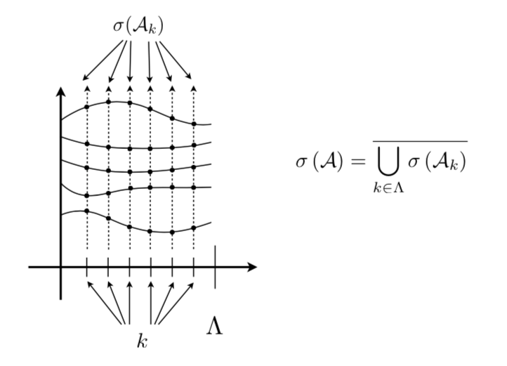
Figure 1: Spectral decomposition for the eigenvalues problem for periodic coefficients differential operators (Bloch-Floquet theorem).

6 Unit-cell and numerical simulations via Bloch-Floquet analysis

In this Section, we perform some discrete numerical simulations of wave dispersion in a precise metamaterial which will be further used to suitably show how the proposed relaxed micromorphic model can describe its (effective) homogenized behavior. Chosen the microstructure, we perform a standard Bloch-Floquet analysis of the wave propagation in the generated periodic infinite medium thanks to the FEM code COMSOL^®. This kind of analysis can be easily implemented using the Bloch-Floquet boundary conditions which are built in the code. The microstructure $\Omega_{c}$ (see Fig.2(b)) we account for is realized as follows: given the plane structure $\Sigma_{c}$ shown in Fig.2(a), with dimensions specified in Table 1, we define $\Omega_{c}=\Sigma_{c}\times\left[0,1\right]$ in which the unit is in meters. The grey region of $\Sigma_{c}$ is filled by aluminum while the white one is empty. The group symmetry of the introduced microstructure is the tetragonal one (the generated solid is invariant under the action of the discrete subgroup $\mathbb{D}_{4}$ of $\textrm{SO}\!\left(3\right)$).

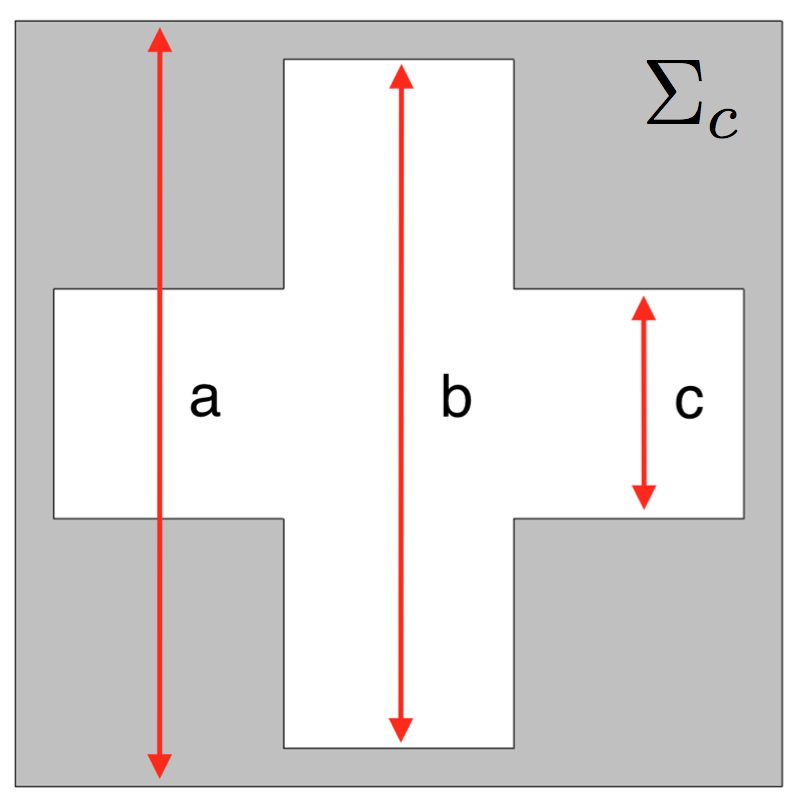
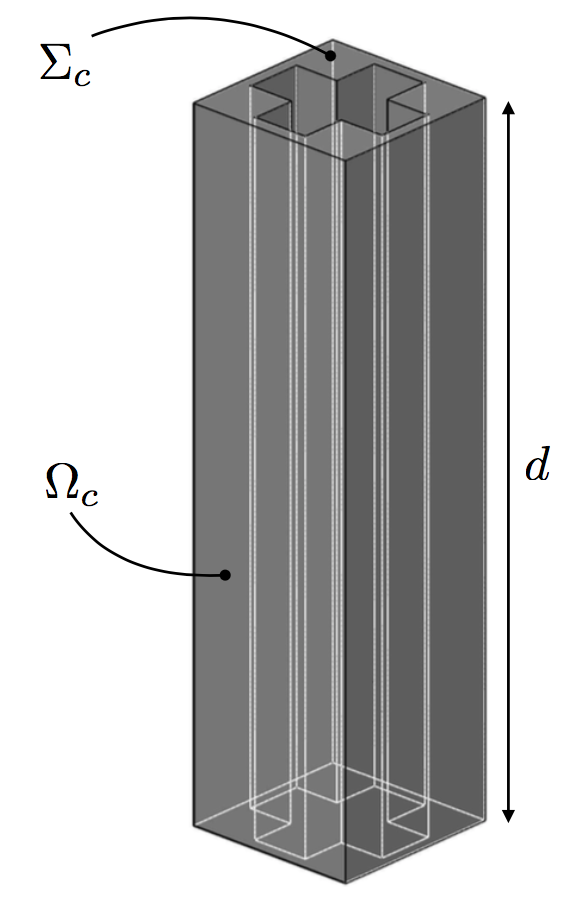
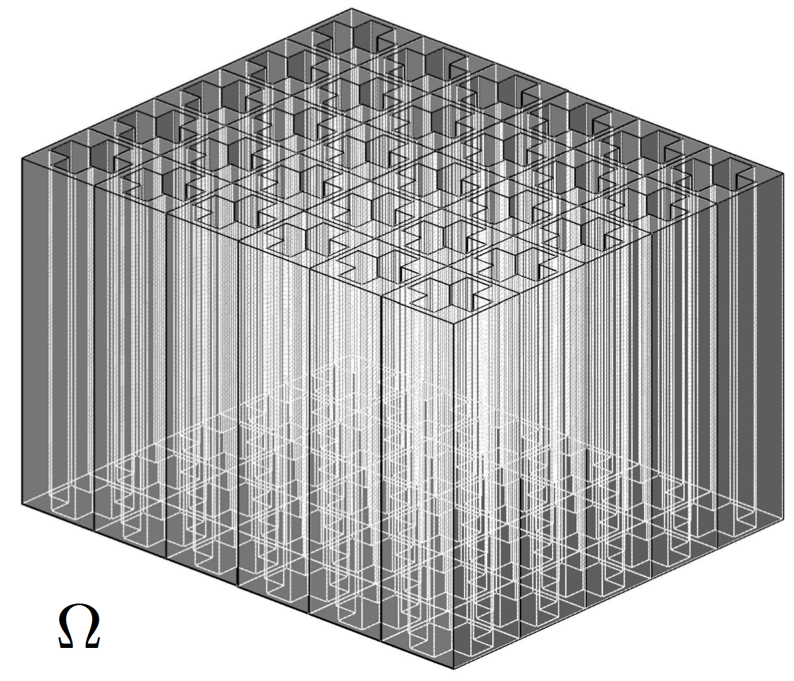
(a)	(b)	(c)

Figure 2: Microstructure implemented in COMSOL^®: (a) Plane cell $\Sigma_{c}$, (b) 3D tetragonal cell $\Omega_{c}$, (c) infinite periodic medium $\Omega$.

The geometric dimensions and the mechanical parameters (Young’s modulus and Poisson’s ratio) of the presented microstructure are given in Table 1.

$a$	$b$	$c$	$d$
$\left[\mathrm{mm}\right]$	$\left[\mathrm{mm}\right]$	$\left[\mathrm{mm}\right]$	$\left[\mathrm{m}\right]$
$1$	$0.9$	$0.3$	$1$

             $E$ $\nu$ $\mu$ $\lambda$ $\left[\mathrm{GPa}\right]$ $-$ $\left[\mathrm{GPa}\right]$ $\left[\mathrm{GPa}\right]$ $70$ $0.33$ $26.32$ $51.08$

Table 1: Geometry of the unit-cell (Fig. 2) and elastic parameters of Aluminum.

We can now determine the apparent density $\rho$ of the unit-cell $\Omega_{c}$. In order to do this, denoting with $V_{\textrm{al}}$ the volume occupied by the aluminum in the unit-cell ($55$%), we find that

$$M_{\textrm{al}}=\rho_{\textrm{al}}V_{\textrm{al}}=2.7\times 10^{3}\times 5.5\times 10^{-7}\left[\frac{\mathrm{kg}}{\mathrm{m}^{3}}\right]\left[\mathrm{m}^{3}\right]=14.85\times 10^{-4}\left[\mathrm{kg}\right],$$

where $M_{\textrm{al}}$ is the mass of the volume occupied by the aluminum and $\rho_{\textrm{al}}=2.7\times 10^{3}\left[\frac{\mathrm{kg}}{\mathrm{m}^{3}}\right]$ is the aluminum mass density. Since the volume of the unit-cell is $\mathit{Vol}\left(\Omega_{c}\right)=10^{-6}\left[\mathrm{m}^{3}\right]$ we find that

$$\rho=\frac{M_{\textrm{al}}}{\mathit{Vol}\left(\Omega_{c}\right)}\left[\frac{\mathrm{kg}}{\mathrm{m}^{3}}\right]=1485\left[\frac{\mathrm{kg}}{\mathrm{m}^{3}}\right].$$ (11)

When fixing the parameters of the unit-cell as in Table 1 and when performing a Bloch-Floquet analysis on the considered periodic structure, the dispersion curves shown in Fig.3 are obtained.

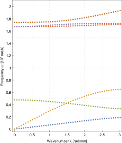
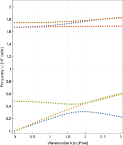
(a)	(b)

Figure 3: COMSOL^® model (plane strain Bloch-Floquet analysis). In (a) we plot the dispersion branches for $\widehat{\boldsymbol{k}}=\left(1,0,0\right)$ (horizontal wave propagation) and in (b) for $\widehat{\boldsymbol{k}}=\left(\sqrt{2}/2,\sqrt{2}/2,0\right)$ (wave propagation at $45\text{\textdegree}$). We observe a band-gap.

These curves for the two directions will be used in Section 8 to fit the dynamical parameters of the relaxed micromorphic model.

7 The tetragonal case in the relaxed micromorphic model

In this Section we are able to illustrate one of the advantages of using the proposed relaxed micromorphic model for the description of the homogenized mechanical behavior of anisotropic metamaterials. Indeed, classical elastic tensors of linear elasticity can be used once the symmetry class of the material is identified. This avoids unnecessary complexifications related to the study of the symmetry classes of higher order tensors as happens, e.g., in gradient elasticity (see, e.g., [5, 41]).

Since the crystallographic symmetry group of $\Omega_{c}$ is $\mathbb{D}_{4}$, we specify the general anisotropic model of a continuum which has the tetragonal symmetry property. This means that all involved structural tensors $\mathbb{C}$ have to respect the invariance condition

$$Q_{ai}Q_{bj}Q_{ch}Q_{dk}\mathbb{C}{}_{abcd}=\mathbb{C}{}_{ijhk},\qquad\forall Q\in\mathbb{D}_{4}.$$ (12)

We express the constitutive tensors as $6\times 6$ matrices with tilde in Voigt notation. In the considered tetragonal case, the matrices corresponding to the considered tensors have the structure (see, e.g., [7]):

$$\widetilde{\mathbb{C}}_{e} =\begin{pmatrix}2\mu_{e}+\lambda_{e}&\lambda_{e}&\lambda_{e}^{*}&0&0&0\\ \lambda_{e}&2\mu_{e}+\lambda_{e}&\lambda_{e}^{*}&0&0&0\\ \lambda_{e}^{*}&\lambda_{e}^{*}&(\widetilde{\mathbb{C}}_{e})_{33}&0&0&0\\ 0&0&0&(\widetilde{\mathbb{C}}_{e})_{44}&0&0\\ 0&0&0&0&(\widetilde{\mathbb{C}}_{e})_{44}&0\\ 0&0&0&0&0&\mu_{e}^{*}\end{pmatrix}, \widetilde{\mathbb{C}}_{c} =\begin{pmatrix}4\mu_{c}^{*}&0&0\\ 0&4\mu_{c}^{*}&0\\ 0&0&4\mu_{c}\end{pmatrix},$$

$$\widetilde{\mathbb{L}} =\begin{pmatrix}2\alpha_{1}+\alpha_{3}&\alpha_{3}&\alpha_{3}^{*}&0&0&0\\ \alpha_{3}&2\alpha_{1}+\alpha_{3}&\alpha_{3}^{*}&0&0&0\\ \alpha_{3}^{*}&\alpha_{3}^{*}&\widetilde{\mathbb{L}}{}_{33}&0&0&0\\ 0&0&0&\widetilde{\mathbb{L}}{}_{44}&0&0\\ 0&0&0&0&\widetilde{\mathbb{L}}{}_{44}&0\\ 0&0&0&0&0&\alpha_{1}^{*}\end{pmatrix}, \widetilde{\mathbb{L}}_{c} =\begin{pmatrix}4\alpha_{2}^{*}&0&0\\ 0&4\alpha_{2}^{*}&0\\ 0&0&4\alpha_{2}\end{pmatrix},$$

$$\widetilde{\mathbb{T}} =\begin{pmatrix}2\overline{\eta}_{1}+\overline{\eta}_{3}&\overline{\eta}_{3}&\overline{\eta}_{3}^{*}&0&0&0\\ \overline{\eta}_{3}&2\overline{\eta}_{1}+\overline{\eta}_{3}&\overline{\eta}_{3}^{*}&0&0&0\\ \overline{\eta}_{3}^{*}&\overline{\eta}_{3}^{*}&\widetilde{\mathbb{T}}{}_{33}&0&0&0\\ 0&0&0&\widetilde{\mathbb{T}}{}_{44}&0&0\\ 0&0&0&0&\widetilde{\mathbb{T}}{}_{44}&0\\ 0&0&0&0&0&\overline{\eta}_{1}^{*}\end{pmatrix}, \widetilde{\mathbb{T}}_{c} =\begin{pmatrix}4\overline{\eta}_{2}^{*}&0&0\\ 0&4\overline{\eta}_{2}^{*}&0\\ 0&0&4\overline{\eta}_{2}\end{pmatrix},$$

$$\widetilde{\mathbb{J}}_{\textrm{micro}} =\begin{pmatrix}2\eta_{1}+\eta_{3}&\eta_{3}&\eta_{3}^{*}&0&0&0\\ \eta_{3}&2\eta_{1}+\eta_{3}&\eta_{3}^{*}&0&0&0\\ \eta_{3}^{*}&\eta_{3}^{*}&(\widetilde{\mathbb{J}}_{\textrm{micro}})_{33}&0&0&0\\ 0&0&0&(\widetilde{\mathbb{J}}_{\textrm{micro}})_{44}&0&0\\ 0&0&0&0&(\widetilde{\mathbb{J}}_{\textrm{micro}})_{44}&0\\ 0&0&0&0&0&\eta_{1}^{*}\end{pmatrix}, \widetilde{\mathbb{J}}_{c} =\begin{pmatrix}4\eta_{2}^{*}&0&0\\ 0&4\eta_{2}^{*}&0\\ 0&0&4\eta_{2}\end{pmatrix},$$ (13)

$$\widetilde{\mathbb{C}}_{\textrm{micro}} =\begin{pmatrix}2\,\mu_{\textrm{micro}}+\lambda_{\textrm{micro}}&\lambda_{\textrm{micro}}&\lambda_{\textrm{micro}}^{*}&0&0&0\\ \lambda_{\textrm{micro}}&2\,\mu_{\textrm{micro}}+\lambda_{\textrm{micro}}&\lambda_{\textrm{micro}}^{*}&0&0&0\\ \lambda_{\textrm{micro}}^{*}&\lambda_{\textrm{micro}}^{*}&(\widetilde{\mathbb{C}}_{\textrm{micro}})_{33}&0&0&0\\ 0&0&0&(\widetilde{\mathbb{C}}_{\textrm{micro}})_{44}&0&0\\ 0&0&0&0&(\widetilde{\mathbb{C}}_{\textrm{micro}})_{44}&0\\ 0&0&0&0&0&\mu_{\textrm{micro}}^{*}\end{pmatrix}.$$

Remark 1.

In the considered plane strain 2D case (no micro and macro motion in the 3-direction) some of the components of the elastic tensors do explicitly appear neither in the PDEs (5) nor in the algebraic system (4.1). This is equivalent to say that, in the considered 2D tetragonal case, the only active components of the involved elastic tensors can be identified as follows:

$$\widetilde{\mathbb{C}}_{e}=\begin{pmatrix}2\mu_{e}+\lambda_{e}&\lambda_{e}&\star&0&0&0\\ \lambda_{e}&2\mu_{e}+\lambda_{e}&\star&0&0&0\\ \star&\star&\star&0&0&0\\ 0&0&0&\star&0&0\\ 0&0&0&0&\star&0\\ 0&0&0&0&0&\mu_{e}^{*}\end{pmatrix}, \widetilde{\mathbb{C}}_{c}=\begin{pmatrix}\star&0&0\\ 0&\star&0\\ 0&0&4\mu_{c}\end{pmatrix}.$$ (14)

Thus, we may arrange the elasticity tensor for our purpose as

$$\begin{pmatrix}2\mu_{e}+\lambda_{e}&\lambda_{e}&0\\ \lambda_{e}&2\mu_{e}+\lambda_{e}&0\\ 0&0&\mu_{e}^{*}\end{pmatrix}$$ (15)

acting only on $\left(\varepsilon_{11},\varepsilon_{22},\varepsilon_{12}\right)$. A similar reducibility holds for the other involved tensors.

8 Fitting material parameters and analysis of dispersion curves

In this Section we will show how:

• thanks to the general anisotropic micro-macro homogenization formula developed in [7] it is possible to establish a functional dependence between the components of the tensors $\mathbb{C}_{e}$ and $\mathbb{C}_{\textrm{micro}}$ appearing in the relaxed micromorphic model and those of the elastic macroscopic elasticity tensor $\mathbb{C}_{\textrm{macro}}$ of the effective (Cauchy) relaxed micromorphic limit model when considering the tetragonal case. Since $\mathbb{C}_{\textrm{micro}}$ and $\mathbb{C}_{\textrm{macro}}$ are known from static arguments, as shown in [30], $\mathbb{C}_{e}$ can be readily computed,

• the calculation of the cut-off frequencies provides the possibility to obtain four extra relations between the micro elastic parameters and the micro inertia terms, thus finally allowing the computation of the micro inertiae and of the Cosserat couple modulus $\mu_{c}$.

8.1 Micro-macro homogenization formula

We now specialize the tensorial micro-macro homogenization formulas obtained in [7, 31, 29] for the general anisotropic framework to the tetragonal case. To this aim, we start counting the parameters of the relaxed micromorphic model for the tetragonal case, which are $\left(\mu_{e},\lambda_{e},\mu_{e}^{*},\mu_{c},\mu_{\textrm{micro}},\lambda_{\textrm{micro}},\mu_{\textrm{micro}}^{*},\mu_{\textrm{macro}},\lambda_{\textrm{macro}},\mu_{\textrm{macro}}^{*},L_{c},\alpha_{1},\alpha_{2},\alpha_{3},\alpha_{1}^{*}\right)$ for the potential part of the energy and $\left(\rho,\eta_{1},\eta_{2},\eta_{3},\eta_{1}^{*},\overline{\eta}_{1},\overline{\eta}_{2},\overline{\eta}_{3},\overline{\eta}_{1}^{*}\right)$ for the kinetic one, then we use the fundamental homogenization formula found in [7]. In [7] it is shown that in the limit $L_{c}\rightarrow 0$ it is possible to homogenize the relaxed micromorphic model to a Cauchy one whose elastic (macroscopic) stiffness $\mathbb{C}_{\textrm{macro}}$ is linked to the relaxed micromorphic material parameters, $\mathbb{C}_{\textrm{micro}},\mathbb{C}_{e}$ by the relation

$$\mathbb{C}_{\textrm{macro}} =\mathbb{C}_{\textrm{micro}}\left(\mathbb{C}_{\textrm{micro}}+\mathbb{C}_{e}\right)^{-1}\mathbb{C}_{e} \Longleftrightarrow \mathbb{C}_{e} =\mathbb{C}_{\textrm{micro}}\left(\mathbb{C}_{\textrm{micro}}-\mathbb{C}_{\textrm{macro}}\right)^{-1}\mathbb{C}_{\textrm{macro}},$$ (16)

which, in our tetragonal case, leads to the identities

$$\mu_{\textrm{macro}} =\frac{\mu_{e}\,\mu_{\textrm{micro}}}{\mu_{e}+\mu_{\textrm{micro}}}, \!\!\!\!\!2\mu_{\textrm{macro}}+3\lambda_{\textrm{macro}} =\frac{\left(2\mu_{e}+3\lambda_{e}\right)\left(2\mu_{\textrm{micro}}+3\lambda_{\textrm{micro}}\right)}{2\left(\mu_{e}+\mu_{\textrm{micro}}\right)+3\left(\lambda_{e}+\lambda_{\textrm{micro}}\right)}, \!\!\!\!\!\mu_{\textrm{macro}}^{*} =\frac{\mu_{e}^{*}\,\mu_{\textrm{micro}}^{*}}{\mu_{e}^{*}+\mu_{\textrm{micro}}^{*}},$$

$$\Longleftrightarrow$$ (17)

$$\mu_{e} =\frac{\mu_{\textrm{macro}}\,\mu_{\textrm{micro}}}{\mu_{\textrm{micro}}-\mu_{\textrm{macro}}}, \!\!\!\!\!2\mu_{e}+3\lambda_{e} =\frac{\left(2\mu_{\textrm{macro}}+3\lambda_{\textrm{macro}}\right)\left(2\mu_{\textrm{micro}}+3\lambda_{\textrm{micro}}\right)}{\left(2\mu_{\textrm{micro}}+3\lambda_{\textrm{micro}}\right)-\left(2\mu_{\textrm{macro}}+3\lambda_{\textrm{macro}}\right)}, \!\!\!\!\!\mu_{e}^{*} =\frac{\mu_{\textrm{macro}}^{*}\,\mu_{\textrm{micro}}^{*}}{\mu_{\textrm{micro}}^{*}-\mu_{\textrm{macro}}^{*}}.$$

Equations (17) give the explicit relations between the parameters of the tetragonal relaxed micromorphic model and the corresponding macroscopic parameters of the Cauchy model seen as a limiting case of the relaxed micromorphic model when $L_{c}\rightarrow 0$, see [30] for further explanations.

The importance of this micro-macro homogenization formula can hardly be overestimated. Indeed, it allows for calibrating the a priori unknown material parameters of the linear relaxed micromorphic model $\mathbb{C}_{e}$ against the in principle known and measurable macroscopic response $\mathbb{C}_{\textrm{macro}}$ and microscopic response $\mathbb{C}_{\textrm{micro}}$. In our case, $\mathbb{C}_{\textrm{macro}}$ has been obtained via numerical homogenization of periodic media (see [30]). On the other hand, $\mathbb{C}_{\textrm{macro}}$ could equivalently be determined from a comparison with the Bloch-Floquet analysis (see also [45] for a good review about homogenization techniques in this context). More precisely, it is well known that the macroscopic parameters $\mu_{\textrm{macro}},\lambda_{\textrm{macro}}$ and $\mu_{\textrm{macro}}^{*}$ can be directly related to the slopes of the acoustic branches of a Cauchy continuum with tetragonal symmetry, and this will allow the determination of the macro parameters for the given metamaterial. We have checked that the macro parameters obtained with the two methods turn out to be the same.

The clear physical interpretation of the micro stiffnesses $\mathbb{C}_{\textrm{micro}}$, on the other hand, is more complicated. Indeed, we know that such micro stiffnesses must be related to the mechanical properties of the unit-cell and true experimental static tests should be run on a specimen composed by a single unit-cell in order to obtain their values. As we explained in [30], different stiffnesses of the unit-cell can be obtained when changing the representative unit-cell for the same metamaterial. However, we established rigorously that the elastic parameters of the stiffest response on the micro-scale must be chosen as $\mathbb{C}_{\textrm{micro}}$.

Once the macro and micro parameters $\mathbb{C}_{\textrm{macro}}$ and $\mathbb{C}_{\textrm{micro}}$ have been determined, the micro-macro homogenization formula (16) allows us to uniquely determine the stiffness $\mathbb{C}_{e}$ which realizes the transition between the macro and micro scale. In particular, for the considered tetragonal metamaterial, and considering the values of $\mathbb{C}_{\textrm{macro}}$ and $\mathbb{C}_{\textrm{micro}}$ given in [30], the values of $\mathbb{C}_{e}$ given in Table 2 can be easily computed through the homogenization formula (17).

$\lambda_{e}$	$\mu_{e}$	$\mu_{e}^{*}$
$\left[\textrm{GPa}\right]$	$\left[\textrm{GPa}\right]$	$\left[\textrm{GPa}\right]$
$-\,0.77$	$17.34$	$0.67$

Table 2: Obtained numerical values for the parameters related to the mesoscopic transition scale. The tensor $\mathbb{C}_{e}$ remains positive definite.

8.2 Cut offs for the optic branches

Only the Cosserat couple modulus $\mu_{c}$ remains to be determined as far as the purely elastic parameters are concerned. On the other hand, all the micro inertiae $\eta_{1},\eta_{1}^{*},\eta_{2},\eta_{3},\overline{\eta}_{1},\overline{\eta}_{1}^{*},\overline{\eta}_{2},\overline{\eta}_{3}$ appearing in the kinetic energy (3) remain to be determined as well. To this aim we consider the so-called cut-off frequencies. Solving the equation $\det\widetilde{D}=0$ imposing that $k=0$, we find the following characteristic frequencies:

$$\omega_{r} =\sqrt{\frac{\mu_{c}}{\eta_{2}}}, \omega_{s} =\sqrt{\frac{\mu_{e}+\mu_{\textrm{micro}}}{\eta_{1}}}, \omega_{s}^{*} =\sqrt{\frac{\mu_{e}^{*}+\mu_{\textrm{micro}}^{*}}{\eta_{1}^{*}}}, \omega_{p} =\sqrt{\frac{\mu_{e}+\mu_{\textrm{micro}}+\lambda_{e}+\lambda_{\textrm{micro}}}{\eta_{1}+\eta_{3}}}.$$ (18)

Such characteristic frequencies correspond to the starting point $\left(k=0\right)$ of the dispersion curves and are known as cut-off frequencies. They are independent of the wave direction.

The simple fact of imposing that such characteristic frequencies are equal to the numerical values of the cut-offs calculated via the Bloch-Floquet analysis (see Fig.(3)) allows us to establish specific relations for computing some of the parameters of the relaxed micromorphic model which are still free. In particular, as we will show in the next Section, the last three formulas of equation (18) enable us to compute $\eta_{1},\eta_{1}^{*}$ and $\eta_{3}$.

8.3 Fitting of the parameters on the dispersion curves

In this Section we show the fitting procedure that we used to calibrate the remaining free parameters of our relaxed micromorphic model on the metamaterial introduced in Section 6. To do so, we denote by $\overline{\omega}_{r},\overline{\omega}_{s},\overline{\omega}_{p}$ and $\overline{\omega}_{s}^{*}$ the numerical values of the cut-offs calculated by the Bloch-Floquet analysis. Moreover, we also denote by $\overline{a}_{\textrm{L}}$ and $\overline{a}_{\textrm{T}}$ the numerical values of the slopes of the tangents to the acoustic curves obtained via the Bloch-Floquet analysis. Note again that the third (out-of-plane) acoustic branch is not present in this case since we implemented a Bloch-Floquet analysis of a fully 2D metamaterial. In Fig. 4 we identify such numerical quantities.

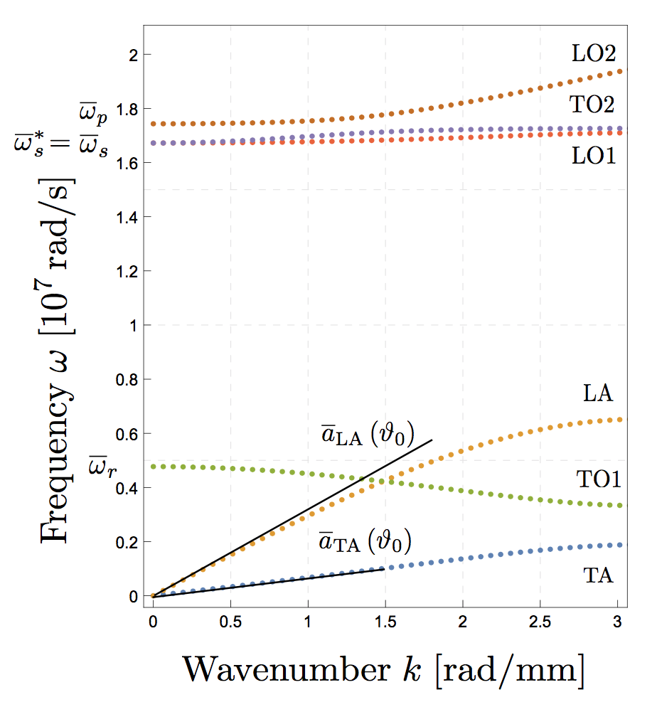
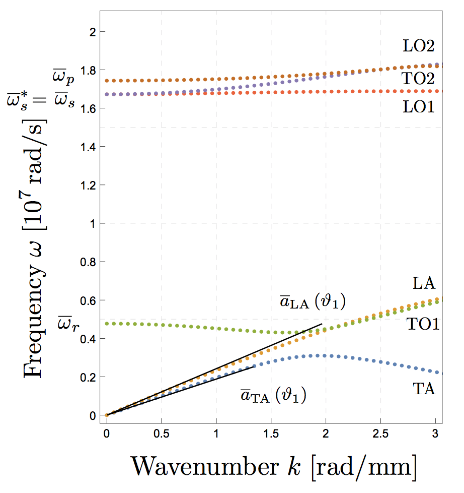
Figure 4: Dispersion curves of the selected metamaterial (for the two directions $\vartheta=\vartheta_{0}=0$ and $\vartheta=\vartheta_{1}=\pi/4$) and identification of the key numerical quantities needed for the fitting procedure. The cut off frequency $\omega_{r},\omega_{s},\omega_{s}^{*}$ and $\omega_{p}$ are direction independent, while the tangents to the acoustic curves $\overline{a}_{\textrm{TA}}$ and $\overline{a}_{\textrm{LA}}$ depend on the direction of wave propagation.

The numerical values of the cut-off frequencies corresponding to Fig. 4 are given in Table 3.

$\overline{\omega}_{r}$	$\overline{\omega}_{s}$	$\overline{\omega}_{s}^{*}$	$\overline{\omega}_{p}$
$\left[\mathrm{rad/s}\right]$	$\left[\mathrm{rad/s}\right]$	$\left[\mathrm{rad/s}\right]$	$\left[\mathrm{rad/s}\right]$
$0.43\cdot 10^{7}$	$1.68\cdot 10^{7}$	$1.68\cdot 10^{7}$	$1.75\cdot 10^{7}$

Table 3: Numerical values of the cut-offs for the considered metamaterial.

Replacing in the last three equations (18) the values of the cut-off frequencies given in Table 3 as well as the values of the elastic parameters given in Table 4b and 2, we can uniquely determine $\eta_{1},\eta_{1}^{*}$ and $\eta_{3}$, obtaining the values in Table 4a.

$\eta_{1}$	$\eta_{3}$	$\eta_{1}^{*}$
$\left[\mathrm{kg/m}\right]$	$\left[\mathrm{kg/m}\right]$	$\left[\mathrm{kg/m}\right]$
$9.3\cdot 10^{-5}$	$0.97\cdot 10^{-5}$	$3.19\cdot 10^{-5}$
	(a)

$\lambda_{\textrm{micro}}$	$\mu_{\textrm{micro}}$	$\mu_{\textrm{micro}}^{\ast}$
$\left[\textrm{GPa}\right]$	$\left[\textrm{GPa}\right]$	$\left[\textrm{GPa}\right]$
$5.27$	$8.93$	$8.33$
	(b)

Table 4: Numerical values for (a) micro inertia parameters and (b) the $\mathbb{C}_{\textrm{micro}}$ parameters.

The parameters of the relaxed micromorphic model which remain free after these considerations are $\eta_{2},\overline{\eta}_{1},\overline{\eta}_{2},\overline{\eta}_{3},\overline{\eta}_{1}^{*}$. To complete the fitting procedure, we start slowly increasing these free parameters, starting from zero, so as to optimally fit dispersion curves of Fig. 4 both for $\vartheta=0$ and $\vartheta=\pi/4$. The order with which the free inertia parameters are increased is related to the effect that such parameters have on the dispersion curves. More particularly:

• $\eta_{2}$ and $\overline{\eta}_{2}$ have an effect on the acoustic curves $\mathrm{LA}$ and $\mathrm{TA}$ and are adjusted to best fit such curves,

• the remaining parameters $\overline{\eta}_{1},\overline{\eta}_{1}^{*},\overline{\eta}_{3}$ are eventually increased only for fine-tuning the fitting. Their effect is mainly visible for higher wavenumber (smaller wavelength).

As for the characteristic length $L_{c}$, we set here $L_{c}=0$. Nevertheless, we know that a non-vanishing $L_{c}$ is a crucial point for a finer fitting of the dispersion curves. On the other hand, this task is really delicate and we need to postpone it to a further work where a micro-inertia related to $\textrm{Curl }P_{,t}$ will also be introduced.

Summarizing the results obtained up to now, we show in Table 5 the values for the inertiae and in Table 6 a summary of all the elastic parameters computed before.

$\rho$	$\eta_{1}$	$\eta_{2}$	$\eta_{3}$	$\eta_{1}^{*}$	$\overline{\eta}_{1}$	$\overline{\eta}_{2}$	$\overline{\eta}_{3}$	$\overline{\eta}_{1}^{*}$
$\left[\mathrm{kg/m}^{3}\right]$	$\left[\mathrm{kg/m}\right]$	$\left[\mathrm{kg/m}\right]$	$\left[\mathrm{kg/m}\right]$	$\left[\mathrm{kg/m}\right]$	$\left[\mathrm{kg/m}\right]$	$\left[\mathrm{kg/m}\right]$	$\left[\mathrm{kg/m}\right]$	$\left[\mathrm{kg/m}\right]$
$1485$	$9.3\cdot 10^{-5}$	$1\cdot 10^{-7}$	$0.97\cdot 10^{-5}$	$3.19\cdot 10^{-5}$	$4.8\cdot 10^{-5}$	$0$	$0$	$0$

Table 5: Summary of the numerical values for inertia parameters.

$\lambda_{e}$ $\mu_{e}$ $\mu_{e}^{*}$ $\left[\textrm{GPa}\right]$ $\left[\textrm{GPa}\right]$ $\left[\textrm{GPa}\right]$ $-\,0.77$ $17.34$ $0.67$

$\lambda_{\textrm{micro}}$ $\mu_{\textrm{micro}}$ $\mu_{\textrm{micro}}^{*}$ $\left[\textrm{GPa}\right]$ $\left[\textrm{GPa}\right]$ $\left[\textrm{GPa}\right]$ $5.27$ $8.93$ $8.33$

$\mu_{c}$ $\left[\textrm{GPa}\right]$ $1.85\cdot 10^{-3}$

$\lambda_{\textrm{macro}}$ $\mu_{\textrm{macro}}$ $\mu_{\textrm{macro}}^{*}$ $\left[\textrm{GPa}\right]$ $\left[\textrm{GPa}\right]$ $\left[\textrm{GPa}\right]$ $1.74$ $5.89$ $0.62$

Table 6: Summary of the numerical values for the elastic parameters of the tetragonal relaxed micromorphic model in 2D. The macroscopic parameters of the resulting homogenized metamaterial are also provided in the last Table. The values related to $\mathbb{C}_{e}$ still define a positive definite tensor.

In Fig. 5 we show the obtained fitting for $\vartheta=0$ and $\vartheta=\pi/4$.

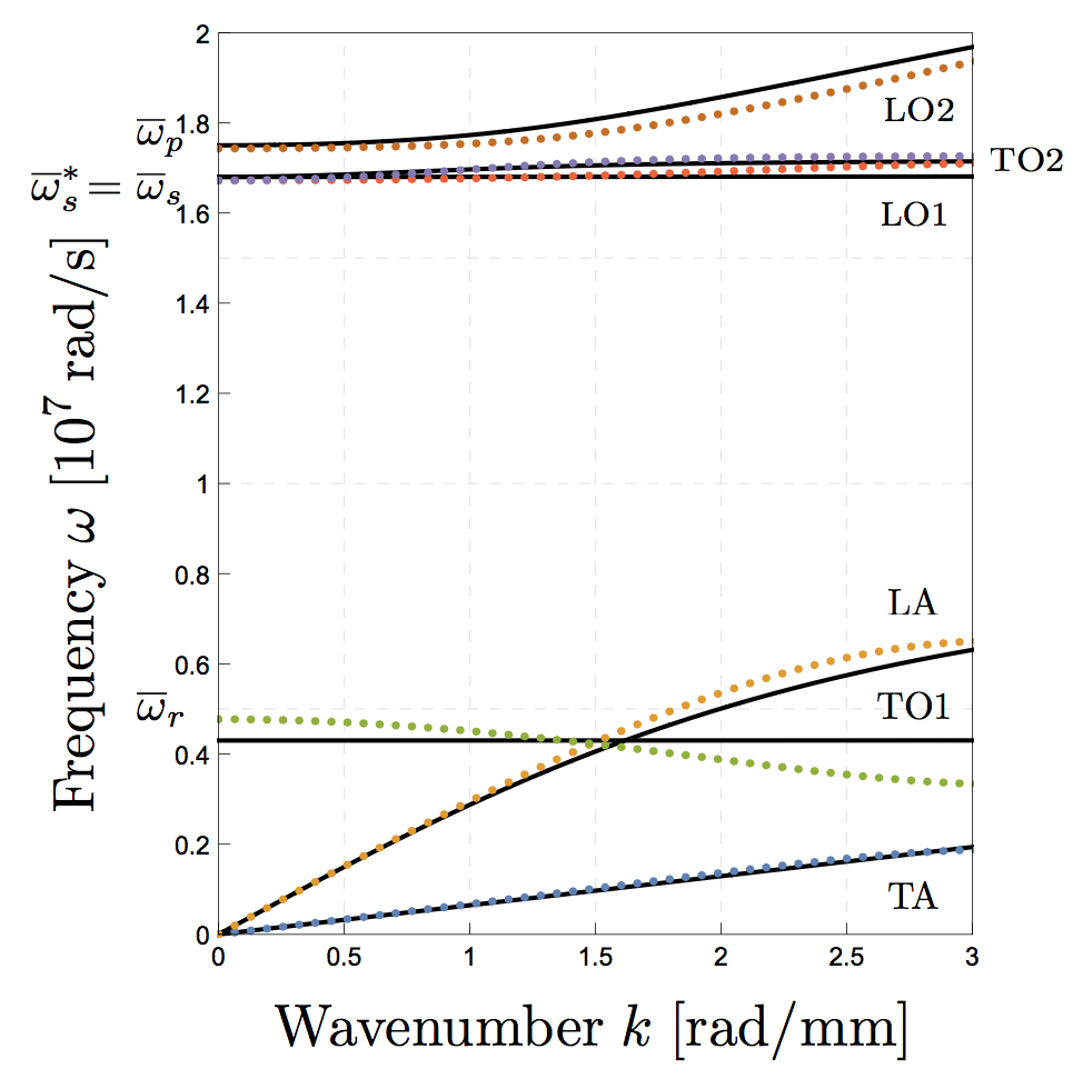
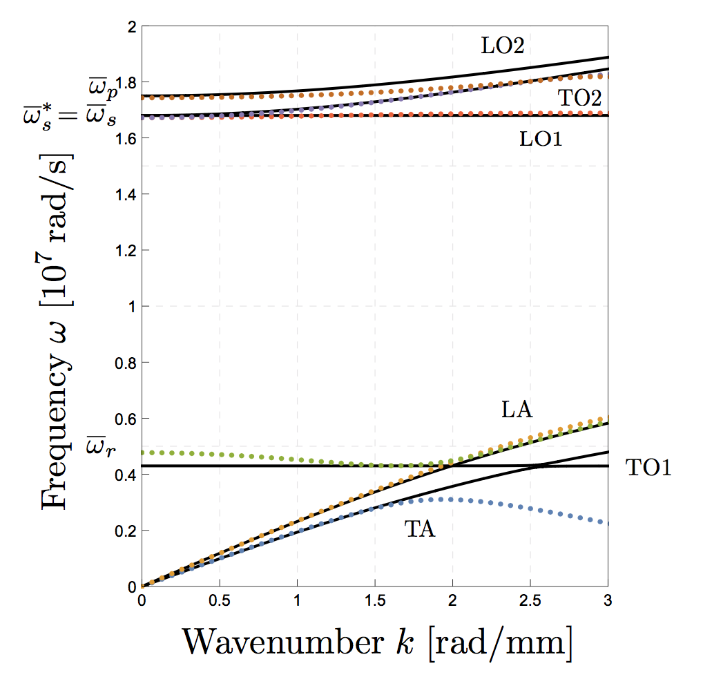
(a)	(b)

Figure 5: Comparison between our relaxed micromorphic continuum model and the COMSOL^® one. In (a) we plot the dispersion branches for $\widehat{\boldsymbol{k}}=\left(1,0,0\right)$ and in (b) for $\widehat{\boldsymbol{k}}=\left(\sqrt{2}/2,\sqrt{2}/2,0\right)$. Dotted lines represent COMSOL^® dispersion curves, continuous lines represent the dispersion curves obtained with the relaxed micromorphic model. The two directions $\widehat{\boldsymbol{k}}$ are used in the fitting procedure.

The result is quite satisfactory for a wide range of wavelengths. The only relevant differences can be found in the curve $\mathrm{TO}_{1}$ both for $\vartheta=0$ and $\vartheta=\pi/4$ and $\mathrm{TA}$ at $\vartheta=\pi/4$. This discrepancy is mainly due to the fact that at present the relaxed micromorphic model is not yet able to give rise to decreasing dispersion curves. Such possibility will be taken into account in future work by adding suitably non-local terms in the kinetic energy and considering $L_{c}>0$.

The parameter calibration that we present in Section 7 is the most natural and simple approach imaginable using enriched continuum models. Indeed, the elastic parameters are calibrated on simple mechanical tests on both macro and micro specimens of the considered metamaterial. On the other hand, dynamical parameters (micro-inertiae) are determined by imposing simple relations on the cut-off frequencies. After that, very few parameters remain free and they are slowly varied to improve the fitting of the dispersion curves at higher wavenumbers (small wavelengths). We claim that we are providing a transparent and efficient characterization of the considered mechanical metamaterial by means of an enriched continuum model.

Our method is physics-based and it is far-away from parameter fittings that are often provided when dealing with the superposition of generalized continuum models to phenomenological data: we do not need to calibrate a huge number of parameters by using “ad hoc” optimization methods, we just obtain the fitting as a simple consequence of our mechanical observations.

We also remark that slight differences can be found in the fitting for some of the higher optic curves when considering high wavenumbers (wavelength smaller than twice the unit-cell), while in general most of the dispersion curves fit well the overall behavior also for wavelength which go down to the size of the unit-cell. We will show in further works that generalizing the expression of the kinetic energy will allow to obtain an even better fitting for the whole considered range of wavelengths.

9 Prediction of dispersion and anisotropy in tetragonal metamaterials

In this Section we show the capability of the anisotropic relaxed micromorphic model to describe complex phenomena in specific metamaterials. We have already seen in Section 6 that the metamaterial targeted in this paper has a tetragonal symmetry. Moreover, in Section 8 we have developed the procedure allowing to calibrate the material parameters of the relaxed micromorphic model on the considered metamaterial.

In the present Section, we show that the relaxed micromorphic model, as calibrated on the considered tetragonal metamaterial, is able to simultaneously reproduce very complex observable macroscopic phenomena, namely

• the dispersive behavior both for the acoustic and the optic curves,

• anisotropic (tetragonal) mechanical behavior of the considered metamaterial for the first six modes.

The first characteristic, i.e., the dispersive behavior of the metamaterial, has already been underlined in the previous Section when noticing that the dispersion curves are not straight lines, but curves. This means that the speed of propagation of each mode is not a constant (as is the case in classical Cauchy continua) but varies when changing the wavelength of the travelling wave. We show again in this Section how the dispersive behavior of the considered metamaterial can be highlighted by introducing the concept of phase velocity. The phase velocity is defined as the ratio $\omega\left(k\right)/k$ and, in dispersive media, changes when changing the wavenumber (or equivalently the wavelength).

The phase velocity also changes when changing the direction of propagation of the travelling wave if the considered medium is not isotropic. Both such features of the phase velocity are easily understandable since:

• the speed of propagation of waves reasonably changes when the travelling wave reaches a wavelength which is comparable to the characteristic size of the underlying microstructure. Such wavelength are easily attainable for the most common metamaterials for which the microstructure has typically the size of millimeters or more,

• if the medium is anisotropic, i.e., if its deformation response varies when varying the direction of application of the external load, it is clear that the speed of propagation of waves inside the medium changes as well when changing the direction of propagation of the travelling wave itself.

We can simultaneously show both such characteristics (anisotropy and dispersion) by looking at the polar plots of the phase velocity $\omega\left(k\right)/k$ for each mode and for different values of the wavenumber $k$ and of the angle $\vartheta$ giving the direction of propagation of the travelling wave.

We start presenting the case of a classical tetragonal non-dispersive Cauchy medium (see Fig. 6).

limit macroscopic Cauchy model

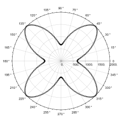
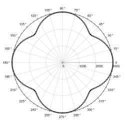
TA	LA

Figure 6: Polar plots of the phase velocity $\omega/k$ for the two acoustic modes of the equivalent tetragonal Cauchy medium, the elastic parameters of which are related to those of the relaxed micromorphic model through formulas (17) and using the values given in Table 6. In each plot, each radial line from zero indicates the direction of propagation of the travelling wave and the length of any segment going from zero to a point of the curve is the measure of the phase velocity $\omega/k$ in the considered direction.

In Fig. 6 we show the polar plots of the phase velocity $\omega/k$ for the tetragonal Cauchy continuum which is obtained as a limiting case of the relaxed micromorphic model as fitted on the considered tetragonal metamaterial. More particularly, Fig. 6 shows that:

1. the two acoustic modes which are described by the Cauchy theory do not describe dispersion. In fact, since in Cauchy theory the dispersion curve is a straight line, once fixed the value of $k$, the phase velocity $\omega/k$ takes a constant value for any chosen value of $k$. It is for this reason that, in Cauchy media, we find only one curve in the polar plot of the phase velocity.

2. Cauchy theory can only describe the first two acoustic modes without any possibility of describing higher modes.

According to these observations, it becomes clear that a Cauchy theory is too restrictive for describing the rich behavior of metamaterials.

As already remarked, second gradient theories could somewhat improve the description of the dispersive behaviors with respect to the Cauchy theory, but in any case only the first 2 modes could be analyzed in the 2D case.

As far as the relaxed micromorphic model is concerned, we will show in the remainder of this Section that it is able to describe:

• not only the first two, but also other modes related to higher frequencies,

• anisotropy, not only for the first two, but also for the other modes,

• dispersion for all the considered modes (here the first 6).

	relaxed micromorphic model	Bloch-Floquet analysis
TA
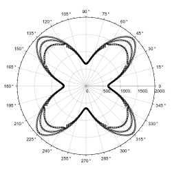
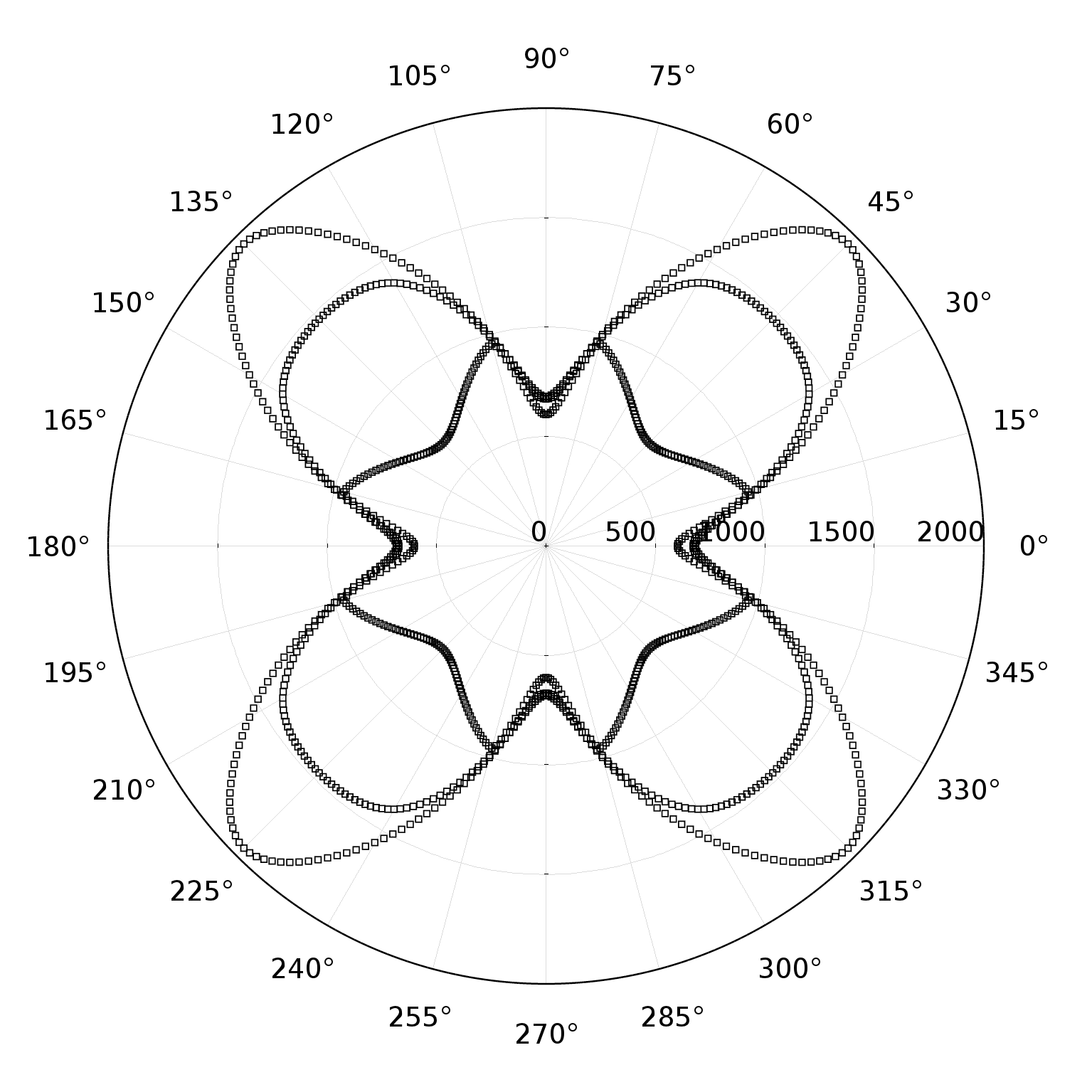
LA
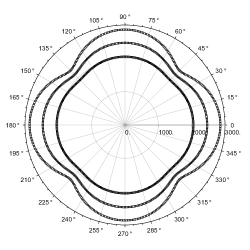
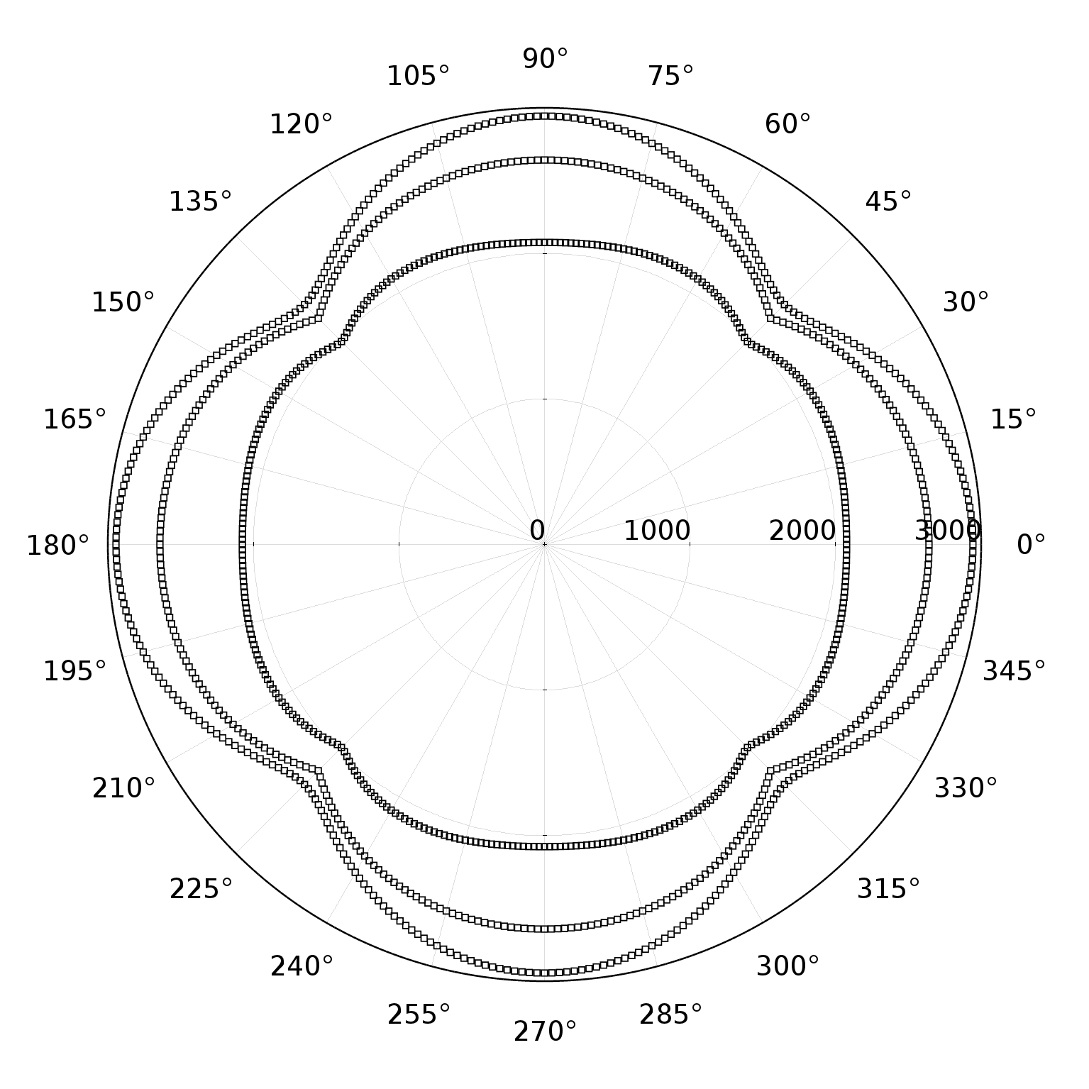
TO1

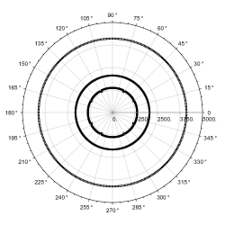
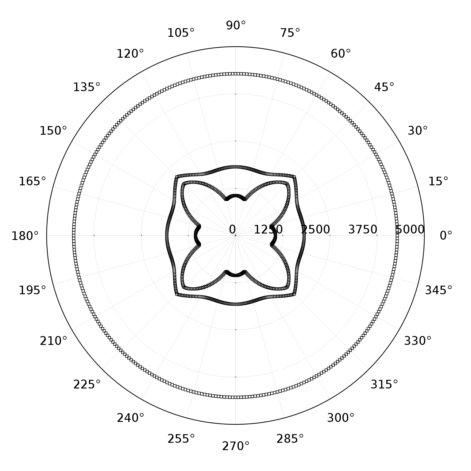
Figure 8: Phase velocity as a function of the direction of wave propagation $\widehat{\boldsymbol{k}}$ for the first three modes as calculated with the relaxed micromorphic model (left) and with the Bloch-Floquet analysis (right). The plotted curves have been calculated for the values of the wave number equal to ${\displaystyle\pi,\frac{2\pi}{3},\frac{\pi}{3}\>\frac{\left[\mathrm{rad}\right]}{\left[\mathrm{mm}\right]}}$ . For any curve, the distance from the center of the circle to a point of the curve itself gives the value of the phase velocity $\omega/k$. More external curves are relative to lower values of $k$, while the curves become closer to the origin when increasing the value of $k$. The most internal curve corresponds to a wavelength comparable to the unit-cell.

We can start remarking from Fig. 8 that the transverse acoustic mode is perfectly described for lower values of $k$ (external curve), while some differences with the Bloch-Floquet analysis of the metamaterial arise for higher values of $k$ (more internal curves).

The larger difference can be detected for waves travelling at $45\text{\textdegree}$. This is consistent with Fig. 5(b) in which it can be easily seen that the transverse wave TA calculated via the relaxed micromorphic model starts diverging from the one calculated via the Block-Floquet analysis when increasing the value of $k$. This means that, as far as the transverse acoustic mode TA is concerned, its description via the relaxed micromorphic model is less accurate when considering propagation at $45\text{\textdegree}$ and higher wavenumbers (smaller wavelengths). As a matter of fact, the description of the TA mode at $45\text{\textdegree}$ starts being less accurate for wavelengths twice the characteristic size of the unit-cell and smaller.

This lack of accuracy for small wavelengths is not present for the longitudinal acoustic mode LA for which the relaxed micromorphic model describes well the behavior of the LA curve for all directions of propagation and for wavelengths which become very small and even comparable to the size of the unit-cell.

The behavior of the curve $\textrm{TO}_{1}$ has to be considered carefully. Indeed, we fitted our relaxed micromorphic model to the $\textrm{TO}_{1}$ dispersion curve with an almost horizontal curve. We are hence able to recover for this mode the average dispersive behavior, but not the true patterns of the phase velocity which show anisotropic behaviors for higher wavenumbers (smaller wavelengths). This behavior will be improved in further works when the non-locality of the matematerial will be considered by considering $L_{c}>0$ and by adding a term $\textrm{Curl}\,P_{,t}$ in the kinetic energy.

We also recall that the relaxed micromorphic model is able to catch some other essential features of the description of the considered metamaterial, such as the presence of band-gaps (see Fig.5).

Based on some preliminary studies, we already know that the typical decreasing behavior of the $\textrm{TO}_{1}$ curve obtained via the Bloch-Floquet analysis can be described by the relaxed micromorphic model if we allow it to include non local effects. In other words, if we consider the case $L_{c}>0$, a better and finer fitting of the $\textrm{TO}_{1}$ curve could be obtained. Nevertheless, the study of this additional case deserves more attention since an extra micro-inertia term involving $\textrm{Curl}\,P_{,t}$ should also be considered. We will hence treat such complete non-local cases in further works, building on the results presented here.

	relaxed micromorphic model	Bloch-Floquet analysis
LO1
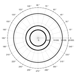
TO2
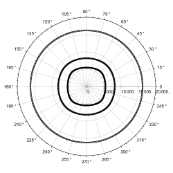
LO2

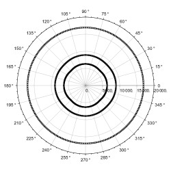
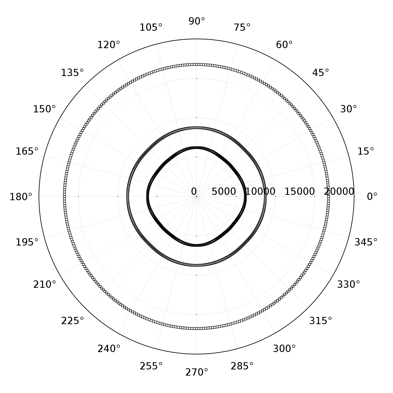
Figure 9: Phase velocity as a function of the direction of wave propagation $\widehat{\boldsymbol{k}}$ for higher modes as calculated with the relaxed micromorphic model (left) and with the Bloch-Floquet analysis (right). The plotted curves have been calculated for the values of the wave number equal to ${\displaystyle\pi,\frac{2\pi}{3},\frac{\pi}{3}\>\frac{\left[\mathrm{rad}\right]}{\left[\mathrm{mm}\right]}}$ . For any curve, the distance from the center of the circle to a point of the curve itself gives the value of the phase velocity $\omega/k$. More external curves are relative to lower values of $k$, while the curves become closer to the origin when increasing the value of $k$. The most internal curve corresponds to a wavelength comparable to the unit-cell.

In Fig. 9 we can see that the relaxed micromorphic model describes almost perfectly both dispersion and anisotropy for the higher optic modes.

10 Conclusion and further perspectives

In this paper we have specialized the general anisotropic relaxed micromorphic model developed in [7] to the case of tetragonal symmetry. We show that this particular symmetry class allows us to describe the anisotropic behavior of a band-gap metamaterial with specific tetragonal microstructure.

We explicitly show the true advantage of using the relaxed micromorphic model [7] in describing the mechanical behavior of metamaterials by introducing only standard fourth order elasticity tensors (in Voigt-notation) as it is the case for classical elasticity. This efficient theoretical framework allows us to avoid unnecessary complexifications related, e.g., to the introduction of elastic tensors of order higher than four, as it is the case for higher gradient elasticity (see, e.g., [6, 37, 36]). Indeed, the study of the anisotropy classes of the tensors appearing in the relaxed micromorphic model follows the classical lines and does not require any extra development.

Then we specialize the anisotropic relaxed micromorphic model to the case of tetragonal symmetry. As a second step, we set up a fitting procedure to determine the values of the parameters of the relaxed micromorphic model by i) computing the purely elastic parameters via suitably conceived static tests in [30] and ii) obtaining the values of dynamical parameters by superimposing the dispersion curves obtained with the relaxed micromorphic model to the corresponding ones obtained with a classical Bloch-Floquet analysis. The relaxed micromorphic model is a “macroscopic continuum” homogenized model which is able to reproduce the response of the selected metamaterial with only few material parameters which do not depend on frequency.

The advantage of our continuum model can be found in the perspective of modeling metamaterials in a simplified framework with transparent mechanical interpretation and thus providing a concrete possibility for the design of relatively complex metastructures by means of a relatively simplified model.

Moreover, the fact that our enriched continuum model is available allows us to simplify the study of other problems that would be otherwise difficult to treat, such as, e.g., the study of interfaces between different anisotropic metamaterials.

The pertinence of the proposed model is shown not only on the dispersion curves but also on the polar plots of the phase velocity which are in good agreement with the analogous results obtained by means of the discrete approach. The few differences that can be found between the discrete and the continuum model are limited to few modes and to high wavenumbers (small wavelengths). Such differences will be treated in future works in which the role of the non-local inertia terms will be investigated together with the case of non-vanishing characteristic length $L_{c}>0$.

Future investigations will also focus on the mechanical characterization of a larger class of band-gap metamaterials with the final aim of the FE-implementation of morphologically complex band-gap metastructures.

Finally, the application of the relaxed micromorphic model to more complex metamaterials including, e.g., piezoelectric effects will also be investigated.

Appendix: equivalent dynamical determination of the macroscopic stiffness $\mathbb{C}_{\textrm{macro}}$

In this appendix we show how the macroscopic parameters previously obtained by simple static arguments can be equivalently computed using the slopes of the acoustic dispersion curves close to the origin. This equivalent method is very useful to make a strong connection between the relaxed micromorphic model and classical elasticity, but it does not add any extra feature to the fitting procedure presented above.

Tangents in zero to the acoustic branches

Let us consider the “macroscopic” Cauchy partial differential system of equations

$$\rho\,u_{,tt}-\textrm{Div}\left(\mathbb{C}_{\textrm{macro}}\,\textrm{sym}\,\nabla u\right)=0$$ (19)

which is the limiting case of the relaxed micromorphic model when $L_{c}$ tends to zero. In this classical case, it is possible to obtain an analytical expression for the dispersion curves. In order to achieve this goal, we enter a generic plane wave function $\widetilde{u}\,e^{\mathfrak{i}\left(\left\langle\boldsymbol{k},x\right\rangle-\omega\,t\right)}$ in (19) obtaining

$$\textrm{Div}\left[\mathbb{C}_{\textrm{macro}}\,\textrm{sym}\,\nabla(\widetilde{u}\,e^{\mathfrak{i}\left(\left\langle\boldsymbol{k},x\right\rangle-\omega\,t\right)})\right] =\left[(\mathbb{C}_{\textrm{macro}})_{ijmn}\,\frac{1}{2}\left(\widetilde{u}_{m}k_{n}+\widetilde{u}_{n}k_{m}\right)\,\mathfrak{i}\,e^{\mathfrak{i}\left(\left\langle\boldsymbol{k},x\right\rangle-\omega\,t\right)}\right]_{,j}$$

$$=-\frac{1}{2}\left[(\mathbb{C}_{\textrm{macro}})_{ijmn}\,\left(\widetilde{u}_{m}k_{n}+\widetilde{u}_{n}k_{m}\right)\,k_{j}\,e^{\mathfrak{i}\left(\left\langle\boldsymbol{k},x\right\rangle-\omega\,t\right)}\right]$$

$$=-\frac{1}{2}\left[\left(\mathbb{C}_{\textrm{macro}}\right)_{ijmn}k_{j}\widetilde{u}_{m}k_{n}+\left(\mathbb{C}_{\textrm{macro}}\right)_{ijmn}k_{j}\widetilde{u}_{n}k_{m}\right]e^{\mathfrak{i}\left(\left\langle\boldsymbol{k},x\right\rangle-\omega\,t\right)}$$ (20)

$$=-\frac{1}{2}\left[\left(\mathbb{C}_{\textrm{macro}}\right)_{ijmn}k_{j}\widetilde{u}_{m}k_{n}+\left(\mathbb{C}_{\textrm{macro}}\right)_{ijnm}k_{j}\widetilde{u}_{n}k_{m}\right]e^{\mathfrak{i}\left(\left\langle\boldsymbol{k},x\right\rangle-\omega\,t\right)}$$

$$=-\left(\mathbb{C}_{\textrm{macro}}\right)_{ijmn}k_{j}\widetilde{u}_{m}k_{n}\,e^{\mathfrak{i}\left(\left\langle\boldsymbol{k},x\right\rangle-\omega\,t\right)},$$

for the static term and

$$\rho\,u_{,tt}=-\rho\,\omega^{2}\,\widetilde{u}\,e^{\mathfrak{i}\left(\left\langle\boldsymbol{k},x\right\rangle-\omega\,t\right)}=-\rho\,\omega^{2}\,\delta_{im}\,\widetilde{u}_{m}e^{\mathfrak{i}\left(\left\langle\boldsymbol{k},x\right\rangle-\omega\,t\right)}$$

for the kinetic term. Thus, finally combining the two expressions we have that $\widetilde{u}\,e^{\mathfrak{i}\left(\left\langle\boldsymbol{k},x\right\rangle-\omega\,t\right)}$ satisfies the system (19) if and only if

$$-\rho\,\omega^{2}\,\delta_{im}\,\widetilde{u}_{m}e^{\mathfrak{i}\left(\left\langle\boldsymbol{k},x\right\rangle-\omega\,t\right)}+\left(\mathbb{C}_{\textrm{macro}}\right)_{ijmn}k_{j}\widetilde{u}_{m}k_{n}\,e^{\mathfrak{i}\left(\left\langle\boldsymbol{k},x\right\rangle-\omega\,t\right)}=0$$

and since the function $e^{\mathfrak{i}\left(\left\langle\boldsymbol{k},x\right\rangle-\omega\,t\right)}$ is always non-zero this gives

$$\left(\rho\,\omega^{2}\,\delta_{im}-\left(\mathbb{C}_{\textrm{macro}}\right){}_{ijmn}k_{j}k_{n}\right)\widetilde{u}_{m}=0$$ (21)

and writing the wave vector as $\boldsymbol{k}=k\,\widehat{\boldsymbol{k}}$ with $\widehat{\boldsymbol{k}}=\big{(}\widehat{k}_{1},\widehat{k}_{2},\widehat{k}_{3}\big{)}$ unitary and $k=\left\|\boldsymbol{k}\right\|$, we arrive to

$$\left(\rho\,\omega^{2}\,\delta_{im}-k^{2}\,\left(\mathbb{C}_{\textrm{macro}}\right){}_{ijmn}\widehat{k}_{j}\widehat{k}_{n}\right)\widetilde{u}_{m}=0.$$ (22)

The equation (22) is an eigenvalues problem for the linear application $k^{2}\,\left(\mathbb{C}_{\textrm{macro}}\right){}_{ijmn}\widehat{k}_{j}\widehat{k}_{n}$. The stated problem admits non-trivial solutions if and only if the determinant of $\rho\,\omega^{2}\,\delta_{im}-k^{2}\,\left(\mathbb{C}_{\textrm{macro}}\right){}_{ijmn}\widehat{k}_{j}\widehat{k}_{n}$ is zero. In this way, we are interested in looking for couples $\left(k,\omega\right)$ such that

$$\det\left(\rho\,\omega^{2}\,\delta_{im}-k^{2}\,\left(\mathbb{C}_{\textrm{macro}}\right){}_{ijmn}\widehat{k}_{j}\widehat{k}_{n}\right)=0.$$ (23)

Moreover, we are interested in studying this problem as a function of the direction of propagation $\widehat{\boldsymbol{k}}$ of the wave. In order to do this, it is convenient to introduce spherical coordinates for the wave vector $\widehat{\boldsymbol{k}}\in\mathbb{S}^{2}$ (the unit sphere in $\mathbb{R}^{3}$):

$$k_{1}=\sin\varphi\,\cos\vartheta,\qquad\qquad k_{2}=\sin\varphi\,\sin\vartheta,\qquad\qquad k_{3}=\cos\varphi,$$ (24)

where $\vartheta\in\left[0,2\pi\right)$ is the polar angle and $\varphi\in\left[0,\pi\right]$ is the azimuthal angle. For the problem in the $\left(x_{1},x_{2},0\right)$ plane, the angle $\varphi$ is $\pi/2$, so

$$k_{1}=\cos\vartheta,\qquad\qquad k_{2}=\sin\vartheta,\qquad\qquad k_{3}=0,$$ (25)

and

$$\widehat{\boldsymbol{k}}\otimes\widehat{\boldsymbol{k}}=\begin{pmatrix}\cos^{2}\vartheta&\cos\vartheta\,\sin\vartheta&0\\ \cos\vartheta\,\sin\vartheta&\sin^{2}\vartheta&0\\ 0&0&0\end{pmatrix}.$$

Let us now consider the Voigt representation of the tensor $\mathbb{C}_{\textrm{macro}}$ in the case of the tetragonal symmetry

$$\widetilde{\mathbb{C}}_{\textrm{macro}}=\begin{pmatrix}2\mu_{\textrm{macro}}+\lambda_{\textrm{macro}}&\lambda_{\textrm{macro}}&\lambda_{\textrm{macro}}^{*}&0&0&0\\ \lambda_{\textrm{macro}}&2\mu_{\textrm{macro}}+\lambda_{\textrm{macro}}&\lambda_{\textrm{macro}}^{*}&0&0&0\\ \lambda_{\textrm{macro}}^{*}&\lambda_{\textrm{macro}}^{*}&(\widetilde{\mathbb{C}}_{\textrm{macro}})_{33}&0&0&0\\ 0&0&0&(\widetilde{\mathbb{C}}_{\textrm{macro}})_{44}&0&0\\ 0&0&0&0&(\widetilde{\mathbb{C}}_{\textrm{macro}})_{44}&0\\ 0&0&0&0&0&\mu_{\textrm{macro}}^{*}\end{pmatrix}.$$

A direct calculation gives

$$\left(\mathbb{C}_{\textrm{macro}}\right){}_{ijmn}\widehat{k}_{j}\widehat{k}_{n}=\left(\begin{array}[]{ccc}\mu_{\textrm{macro}}^{\ast}\,\sin^{2}\vartheta+\cos^{2}\vartheta\left(\lambda_{\textrm{macro}}+2\mu_{\textrm{macro}}\right)&\cos\vartheta\sin\vartheta\left(\mu_{\textrm{macro}}^{\ast}+\lambda_{\textrm{macro}}\right)&0\\ \cos\vartheta\sin\vartheta\left(\mu_{\textrm{macro}}^{\ast}+\lambda_{\textrm{macro}}\right)&\cos^{2}\vartheta\mu_{\textrm{macro}}^{\ast}+\sin^{2}\vartheta\left(\lambda_{\textrm{macro}}+2\mu_{\textrm{macro}}\right)&0\\ 0&0&\big{(}\widetilde{\mathbb{C}}_{\textrm{macro}}\big{)}_{44}\end{array}\right),$$

thus, for $\rho\,\omega^{2}\,\delta_{im}-k^{2}\,\left(\mathbb{C}_{\textrm{macro}}\right){}_{ijmn}\widehat{k}_{j}\widehat{k}_{n}$, we find

$$\!\!\!\!\!\!\!\!\!\!\!\!\!\!\!\!\!\!\!\!\!\!\!\!\left(\begin{array}[]{ccc}\rho\omega^{2}-k^{2}\left(\mu_{\textrm{macro}}^{\ast}\sin^{2}\vartheta+\cos^{2}\vartheta\left(\lambda_{\textrm{macro}}+2\mu_{\textrm{macro}}\right)\right)&-k^{2}\cos\vartheta\sin\vartheta\left(\mu_{\textrm{macro}}^{\ast}+\lambda_{\textrm{macro}}\right)&0\\ -k^{2}\cos\vartheta\sin\vartheta\left(\mu_{\textrm{macro}}^{\ast}+\lambda_{\textrm{macro}}\right)&\rho\omega^{2}-k^{2}\left(\mu_{\textrm{macro}}^{\ast}\cos^{2}\vartheta+\sin^{2}\vartheta\left(\lambda_{\textrm{macro}}+2\mu_{\textrm{macro}}\right)\right)&0\\ 0&0&\rho\omega^{2}-\big{(}\widetilde{\mathbb{C}}_{\textrm{macro}}\big{)}_{44}k^{2}\end{array}\right).$$

In this way we can compute

$$\det\left(\rho\,\omega^{2}\,\delta_{im}-k^{2}\,\left(\mathbb{C}_{\textrm{macro}}\right){}_{ijmn}\widehat{k}_{j}\widehat{k}_{n}\right)=\qquad\qquad\qquad\qquad\qquad\qquad\qquad\qquad\qquad\qquad\qquad\qquad\qquad\qquad$$

$$=\left(\rho\,\omega^{2}-\big{(}\widetilde{\mathbb{C}}_{\textrm{macro}}\big{)}_{44}k^{2}\right)\Big{[}\left(\rho\,\omega^{2}-k^{2}\left(\cos^{2}\vartheta\left(\lambda_{\textrm{macro}}+2\mu_{\textrm{macro}}\right)+\mu_{\textrm{macro}}^{\ast}\sin^{2}\vartheta\right)\right)\qquad\qquad\qquad$$ (26)

$$\left(\rho\,\omega^{2}-k^{2}\left(\sin^{2}\vartheta\left(\lambda_{\textrm{macro}}+2\mu_{\textrm{macro}}\right)+\mu_{\textrm{macro}}^{\ast}\cos^{2}\vartheta\right)\right)-k^{4}\sin^{2}\vartheta\cos^{2}\vartheta\left(\lambda_{\textrm{macro}}+\mu_{\textrm{macro}}^{\ast}\right){}^{2}\Big{]}.$$

The dispersion curves for the classical limit Cauchy model are obtained solving the equation (23), or equivalently (26), with respect to $\omega^{2}$. We call $\left\{\pm\,\omega_{\textrm{macro},i}\left(k,\vartheta\right)\right\}_{i=1}^{3}$ the dispersion curves for the Cauchy continuum obtained by solving (23) for the special tetragonal case given in (26). A direct calculation shows that the positive solutions $\left\{\omega_{\textrm{macro},i}\left(k,\vartheta\right)\right\}_{i=1}^{3}$ of (23) for the tetragonal case are three straight lines in the $\left(\omega,k\right)$ plane with slopes (here, and only here, we use the abbreviations $\mu_{M}=\mu_{\textrm{macro}},$ $\lambda_{M}=\lambda_{\textrm{macro}}$, $\mu_{M}^{*}=\mu_{\textrm{macro}}^{*}$):

$$a_{\mathrm{LA}} =\sqrt{\frac{\lambda_{M}+\mu_{M}^{\ast}+2\mu_{M}+\sqrt{2\cos(4\vartheta)\left(\lambda_{M}+\mu_{M}\right)\left(\mu_{M}-\mu_{M}^{\ast}\right)+2\lambda_{M}\mu_{M}+\lambda_{M}^{2}+\mu_{M}^{\ast 2}-2\mu_{M}\mu_{M}^{\ast}+2\mu_{M}^{2}}}{2\rho}},$$ (27)

$$a_{\mathrm{TA}} =\sqrt{\frac{\lambda_{M}+\mu_{M}^{\ast}+2\mu_{M}-\sqrt{2\cos(4\vartheta)\left(\lambda_{M}+\mu_{M}\right)\left(\mu_{M}-\mu_{M}^{\ast}\right)+2\lambda_{M}\mu_{M}+\lambda_{M}^{2}+\mu_{M}^{\ast 2}-2\mu_{M}\mu_{M}^{\ast}+2\mu_{M}^{2}}}{2\rho}},$$

$$a_{\mathrm{TA}3} =\sqrt{\frac{\left(\widetilde{\mathbb{C}}_{M}\right)_{44}}{\rho}}.$$ (28)

Note the complete absence of the Cosserat couple modulus $\mu_{c}$ in the latter formulas.

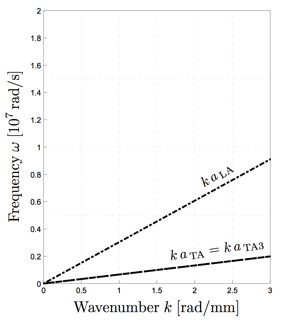
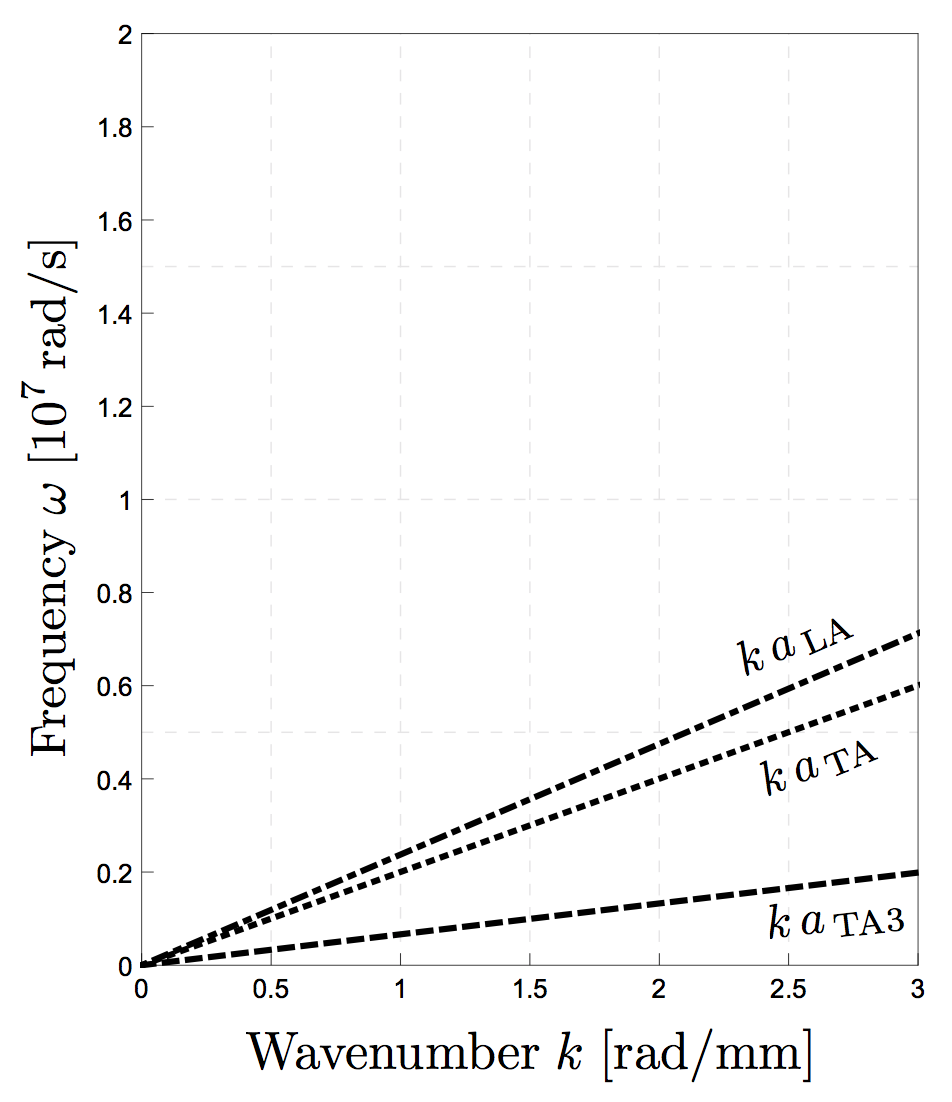
(a)	(b)

Figure 7: Dispersion branches for the limiting tetragonal Cauchy continuum with $\widehat{\boldsymbol{k}}=\left(1,0,0\right)$ (Fig. (a)) and $\widehat{\boldsymbol{k}}=\left(\sqrt{2}/2,\sqrt{2}/2,0\right)$ (Fig. (b)).

Such dispersion curves are called (in-plane) longitudinal-acoustic (LA), (in-plane) transverse-acoustic (TA) and (out-of-plane) transverse-acoustic (TA3). Since in this paper we are interested only in vibrations in the $\left(x_{1},x_{2},0\right)$ plane, the third acoustic line with slope $a_{\mathrm{TA}3}$ will not be considered for the fitting procedure since it corresponds to out-of-plane vibrations.

One remarkable property of the relaxed micromorphic model is that the slopes of its acoustic curves close to the origin, are exactly given by the slopes of the acoustic lines (27) of the equivalent Cauchy continuum. More precisely, the slopes at zero of the acoustic branches of the dispersion curves as obtained via the relaxed micromorphic model can be computed by means of equations (27) when using the identities (17).

Dynamical calculation of the macroscopic stiffness $\mathbb{C}_{\textrm{macro}}$

Based on the results of the previous Paragraph, we can compute the numerical values of the macroscopic parameters $\mu_{\textrm{macro}},\lambda_{\textrm{macro}}$ and $\mu_{\textrm{macro}}^{*}$ which represent the measure of the macroscopic stiffness of the considered tetragonal metamaterial. To this aim, considering the two directions of propagation $\vartheta_{0}=0$ and $\vartheta_{1}=\pi/4$, and accounting for the following assumptions on the involved constitutive parameters

$$\lambda_{\textrm{macro}}>0,\quad\mu_{\textrm{macro}}>0,\quad\mu_{\textrm{macro}}^{*}>0,\quad\lambda_{\textrm{macro}}+2\mu_{\textrm{macro}}-\mu_{\textrm{macro}}^{*}>0,$$

we set up the following system of algebraic equations:

$$a_{\textrm{LA}}\left(\vartheta_{0},\lambda_{\textrm{macro}},\mu_{\textrm{macro}},\mu_{\textrm{macro}}^{*}\right)=\sqrt{\frac{2\mu_{\textrm{macro}}+\lambda_{\textrm{macro}}}{\rho}} =\overline{a}_{\textrm{LA}}\left(\vartheta_{0}\right),$$

$$a_{\textrm{LA}}\left(\vartheta_{1},\lambda_{\textrm{macro}},\mu_{\textrm{macro}},\mu_{\textrm{macro}}^{*}\right)=\sqrt{\frac{\mu_{\textrm{macro}}+\mu_{\textrm{macro}}^{*}+\lambda_{\textrm{macro}}}{\rho}} =\overline{a}_{\textrm{LA}}\left(\vartheta_{1}\right),$$ (29)

$$a_{\textrm{TA}}\left(\vartheta_{0},\lambda_{\textrm{macro}},\mu_{\textrm{macro}},\mu_{\textrm{macro}}^{*}\right)=\sqrt{\frac{\mu_{\textrm{macro}}^{*}}{\rho}} =\overline{a}_{\textrm{TA}}\left(\vartheta_{0}\right),$$

$$a_{\textrm{TA}}\left(\vartheta_{1},\lambda_{\textrm{macro}},\mu_{\textrm{macro}},\mu_{\textrm{macro}}^{*}\right)=\sqrt{\frac{\mu_{\textrm{macro}}}{\rho}} =\overline{a}_{\textrm{TA}}\left(\vartheta_{1}\right).$$

This system of algebraic equations counts 4 equations and 3 unknowns. We use the first 3 equations to calculate the unknowns $\lambda_{\textrm{macro}},\mu_{\textrm{macro}},\mu_{\textrm{macro}}^{*}$ and then plug the found values in the fourth equation.

If our hypothesis according to which the metamaterial we are considering has a tetragonal symmetry is correct, the fourth equation has to be automatically satisfied. This is indeed the case.

The numerical values of the macroscopic parameters which are found with the described procedure are given in Table 7.

Bloch - Floquet		periodic homogenization
$\lambda_{\textrm{macro}}$ $\mu_{\textrm{macro}}$ $\mu_{\textrm{macro}}^{*}$ $\left[\mathrm{GPa}\right]$ $\left[\mathrm{GPa}\right]$ $\left[\mathrm{GPa}\right]$ $1.77$ $5.95$ $0.65$		$\lambda_{\textrm{macro}}$ $\mu_{\textrm{macro}}$ $\mu_{\textrm{macro}}^{*}$ $\left[\textrm{GPa}\right]$ $\left[\textrm{GPa}\right]$ $\left[\textrm{GPa}\right]$ $1.74$ $5.89$ $0.62$

Table 7: Left: numerical values of the macroscopic parameters of the relaxed micromorphic model as obtained via the dynamical fitting and Bloch-Floquet analysis. Right: for comparison the values obtained by periodic homogenization.

References

- [1] Alexios Aivaliotis, Ali Daouadji, Gabriele Barbagallo, Domenico Tallarico, Patrizio Neff, and Angela Madeo. Low-and high-frequency Stoneley waves, reflection and transmission at a Cauchy/relaxed micromorphic interface. arXiv preprint arXiv:1810.12578, 2018.
- [2] Alexios Aivaliotis, Ali Daouadji, Gabriele Barbagallo, Domenico Tallarico, Patrizio Neff, and Angela Madeo. Microstructure-related Stoneley waves and their effect on the scattering properties of a 2d Cauchy/relaxed-micromorphic interface. Wave Motion, 90:99–120, 2019.
- [3] Tryfon Antonakakis, Richard Craster, and Sebastien Guenneau. High-frequency homogenization of zero-frequency stop band photonic and phononic crystals. New Journal of Physics, 15(10):103014, 2013.
- [4] Mario N. Armenise, Carlo E. Campanella, Caterina Ciminelli, Francesco Dell’Olio, and Vittorio M. N. Passaro. Phononic and photonic band gap structures: Modelling and applications. Physics Procedia, 3(1):357–364, 2010.
- [5] Nicolas Auffray. On the algebraic structure of isotropic generalized elasticity theories. Mathematics and Mechanics of Solids, 20(5):565–581, 2015.
- [6] Nicolas Auffray, Hung Le Quang, and Qi-Chang He. Matrix representations for 3d strain-gradient elasticity. Journal of the Mechanics and Physics of Solids, 61(5):1202–1223, 2013.
- [7] Gabriele Barbagallo, Angela Madeo, Marco Valerio d’Agostino, Rafael Abreu, Ionel-Dumitrel Ghiba, and Patrizio Neff. Transparent anisotropy for the relaxed micromorphic model: macroscopic consistency conditions and long wave length asymptotics. International Journal of Solids and Structures, 120:7–30, 2017.
- [8] Gabriele Barbagallo, Domenico Tallarico, Marco Valerio d’Agostino, Alexios Aivaliotis, Patrizio Neff, and Angela Madeo. Relaxed micromorphic model of transient wave propagation in anisotropic band-gap metastructures. International Journal of Solids and Structures, 162:148–163, 2019.
- [9] Felix Bloch. Über die Quantenmechanik der Elektronen in Cristallgittern. Zeitschrift für Physik A Hadrons and Nuclei, 52(7):555–600, 1929.
- [10] Miguel Charlotte and Lev Truskinovsky. Lattice dynamics from a continuum viewpoint. Journal of the Mechanics and Physics of Solids, 60(8):1508–1544, 2012.
- [11] Youping Chen and James D. Lee. Connecting molecular dynamics to micromorphic theory. (I). Instantaneous and averaged mechanical variables. Physica A: Statistical Mechanics and its Applications, 322:359–376, 2003.
- [12] Youping Chen and James D. Lee. Determining material constants in micromorphic theory through phonon dispersion relations. International Journal of Engineering Science, 41(8):871–886, 2003.
- [13] Marco Valerio d’Agostino, Gabriele Barbagallo, Ionel-Dumitrel Ghiba, Rafael Abreu, Angela Madeo, and Patrizio Neff. A panorama of dispersion curves for the isotropic weighted relaxed micromorphic model. Zeitschrift für Angewandte Mathematik und Mechanik, 97(11):1436–1481, 2017.
- [14] Francesco dell’Isola, Angela Madeo, and Luca Placidi. Linear plane wave propagation and normal transmission and reflection at discontinuity surfaces in second gradient 3D continua. Zeitschrift für Angewandte Mathematik und Mechanik, 92(1):52–71, 2012.
- [15] Hao-Wen Dong, Sheng-Dong Zhao, Yue-Sheng Wang, and Chuanzeng Zhang. Topology optimization of anisotropic broadband double-negative elastic metamaterials. Journal of the Mechanics and Physics of Solids, 105:54–80, 2017.
- [16] Ahmed Cemal Eringen. Microcontinuum Field Theories. Springer-Verlag, New York, 1999.
- [17] Claudio Findeisen, Jörg Hohe, Muamer Kadic, and Peter Gumbsch. Characteristics of mechanical metamaterials based on buckling elements. Journal of the Mechanics and Physics of Solids, 102:151–164, 2017.
- [18] Gaston Floquet. Sur les equations differentielles lineaires. Ann. Ecole Normale Supérieure, 12(1883):47–88, 1883.
- [19] Miroslav Hlaváček. A continuum theory for isotropic two-phase elastic composites. International Journal of Solids and Structures, 11(10):1137–1144, 1975.
- [20] Min Kyung Lee, Pyung Sik Ma, Il Kyu Lee, Hoe Woong Kim, and Yoon Young Kim. Negative refraction experiments with guided shear-horizontal waves in thin phononic crystal plates. Applied Physics Letters, 98(1):011909, 2011.
- [21] Angela Madeo, Gabriele Barbagallo, Marco Valerio d’Agostino, Luca Placidi, and Patrizio Neff. First evidence of non-locality in real band-gap metamaterials: determining parameters in the relaxed micromorphic model. Proceedings of the Royal Society A: Mathematical, Physical and Engineering Sciences, 472(2190):20160169, 2016.
- [22] Angela Madeo, Manuel Collet, Marco Miniaci, Kévin Billon, Morvan Ouisse, and Patrizio Neff. Modeling phononic crystals via the weighted relaxed micromorphic model with free and gradient micro-inertia. Journal of Elasticity, 130:1–25, 2017.
- [23] Angela Madeo, Patrizio Neff, Elias C. Aifantis, Gabriele Barbagallo, and Marco Valerio d’Agostino. On the role of micro-inertia in enriched continuum mechanics. Proc. R. Soc. A, 473(2198):20160722, 2017.
- [24] Angela Madeo, Patrizio Neff, Marco Valerio d’Agostino, and Gabriele Barbagallo. Complete band gaps including non-local effects occur only in the relaxed micromorphic model. Comptes Rendus Mécanique, 344(11):784–796, 2016.
- [25] Angela Madeo, Patrizio Neff, Ionel-Dumitrel Ghiba, Luca Placidi, and Giuseppe Rosi. Band gaps in the relaxed linear micromorphic continuum. Zeitschrift für Angewandte Mathematik und Mechanik, 95(9):880–887, 2014.
- [26] Angela Madeo, Patrizio Neff, Ionel-Dumitrel Ghiba, Luca Placidi, and Giuseppe Rosi. Wave propagation in relaxed micromorphic continua: modeling metamaterials with frequency band-gaps. Continuum Mechanics and Thermodynamics, 27(4-5):551–570, 2015.
- [27] Angela Madeo, Patrizio Neff, Ionel-Dumitrel Ghiba, and Giussepe Rosi. Reflection and transmission of elastic waves in non-local band-gap metamaterials: a comprehensive study via the relaxed micromorphic model. Journal of the Mechanics and Physics of Solids, 95:441–479, 2016.
- [28] Raymond David Mindlin. Micro-structure in linear elasticity. Archive for Rational Mechanics and Analysis, 16(1):51–78, 1964.
- [29] Patrizio Neff. On material constants for micromorphic continua. In Trends in Applications of Mathematics to Mechanics, STAMM Proceedings, Seeheim, pages 337–348. Shaker–Verlag, 2004.
- [30] Patrizio Neff, Bernhard Eidel, Marco Valerio d’Agostino, and Angela Madeo. Identification of scale-independent material parameters in the relaxed micromorphic model through model-adapted first order homogenization. Accepted. Journal of Elasticity, 2019.
- [31] Patrizio Neff and Samuel Forest. A geometrically exact micromorphic model for elastic metallic foams accounting for affine microstructure. Modelling, existence of minimizers, identification of moduli and computational results. Journal of Elasticity, 87(2-3):239–276, 2007.
- [32] Patrizio Neff, Ionel-Dumitrel Ghiba, Angela Madeo, Luca Placidi, and Giuseppe Rosi. A unifying perspective: the relaxed linear micromorphic continuum. Continuum Mechanics and Thermodynamics, 26(5):639–681, 2014.
- [33] Patrizio Neff, Angela Madeo, Gabriele Barbagallo, Marco Valerio d’Agostino, Rafael Abreu, and Ionel-Dumitrel Ghiba. Real wave propagation in the isotropic-relaxed micromorphic model. Proceedings of the Royal Society A: Mathematical, Physical and Engineering Sciences, 473(2197), 2017.
- [34] Sia Nemat-Nasser and Ankit Srivastava. Overall dynamic constitutive relations of layered elastic composites. Journal of the Mechanics and Physics of Solids, 59(10):1953–1965, 2011.
- [35] Sia Nemat-Nasser, John R. Willis, Ankit Srivastava, and Alireza V. Amirkhizi. Homogenization of periodic elastic composites and locally resonant sonic materials. Physical Review B, 83(10):104103, 2011.
- [36] Marc Olive and Nicolas Auffray. Symmetry classes for even-order tensors. Mathematics and Mechanics of Complex Systems, 1(2):177–210, 2013.
- [37] Marc Olive and Nicolas Auffray. Symmetry classes for odd-order tensors. Zeitschrift für Angewandte Mathematik und Mechanik, 94(5):421–447, 2014.
- [38] Sebastian Owczarek, Ionel-Dumitrel Ghiba, Marco-Valerio d’Agostino, and Patrizio Neff. Nonstandard micro-inertia terms in the relaxed micromorphic model: well-posedness for dynamics. Accepted Mathematics and Mechanics of Solids. arXiv preprint arXiv:1809.04791, 2018.
- [39] Luca Placidi, Giuseppe Rosi, Ivan Giorgio, and Angela Madeo. Reflection and transmission of plane waves at surfaces carrying material properties and embedded in second-gradient materials. Mathematics and Mechanics of Solids, 19(5):555–578, 2014.
- [40] Giuseppe Rosi and Nicolas Auffray. Anisotropic and dispersive wave propagation within strain-gradient framework. Wave Motion, 63:120–134, 2016.
- [41] Giuseppe Rosi, Luca Placidi, and Nicolas Auffray. On the validity range of strain-gradient elasticity: a mixed static-dynamic identification procedure. European Journal of Mechanics-A/Solids, 69:179–191, 2018.
- [42] Valery P. Smyshlyaev. Propagation and localization of elastic waves in highly anisotropic periodic composites via two-scale homogenization. Mechanics of Materials, 41(4):434–447, 2009.
- [43] Valery P. Smyshlyaev and Kirill D. Cherednichenko. On rigorous derivation of strain gradient effects in the overall behaviour of periodic heterogeneous media. Journal of the Mechanics and Physics of Solids, 48(6-7):1325–1357, 2000.
- [44] Walter Steurer and Daniel Sutter-Widmer. Photonic and phononic quasicrystals. Journal of Physics D: Applied Physics, 40(13):229–247, 2007.
- [45] Vasilii Vasil’evich Zhikov and Svetlana Evgenievna Pastukhova. Operator estimates in homogenization theory. Russian Mathematical Surveys, 71(3):417, 2016.