Finite lifetime broadening of calculated x-ray absorption spectra: possible artefacts close to the edge

Abstract

X-ray absorption spectra calculated within an effective one-electron approach have to be broadened to account for the finite lifetime of the core hole. For Green’s function based methods this can be achieved either by adding a small imaginary part to the energy or by convoluting the spectra on the real axis with a Lorentzian. We demonstrate on the case of Fe $K$ and $L_{2,3}$ edge spectra that these procedures lead to identical results only for energies higher than few core level widths above the absorption edge. For energies close to the edge, spurious spectral features may appear if too much weight is put on broadening via the imaginary energy component. Special care should be taken for dichroic spectra at edges which comprise several exchange-split core levels, such as the $L_{3}$ edge of 3$d$ transition metals.

I Introduction

Generally, experimental x-ray absorption spectra (XAS) contain fewer structures and display broader features than theoretical spectra. This is because the finite lifetime of the core hole is usually neglected in the calculations. To facilitate proper comparison between theory and experiment, the calculated spectrum is modified so that the finite core hole lifetime is accounted for. A convenient way to achieve this is to convolute the raw spectrum a posteriori with a Lorentzian.Messiah (1962) This is a well-established procedure. Its drawback is that one has to perform the calculations on sometimes much finer energy mesh than actually needed: the raw spectrum contains many fine and sharp features that will be smeared out eventually but which, nevertheless, have to be included in the calculated spectrum before the final broadening is applied.

For Green’s function based or multiple-scattering methods, there is another — computationally more efficient — way to account for the finite core hole lifetime, namely, adding a small imaginary part to the energy.Messiah (1962); Vedrinskii et al. (1982); Brouder et al. (1996); Natoli et al. (2003); Sébilleau et al. (2006) This will result in smoother spectra from the beginning, meaning that one can use a coarser energy mesh (cf. an instructive demonstration presented recently by Taranukhina et al.).Taranukhina et al. (2018) Another technical advantage of this approach from a computational viewpoint is that when working in a reciprocal space, employing complex energies may significantly reduce the number of $\bm{k}$-points needed for an accurate Brillouin zone integration. The option to use complex energies is available in several codes designed for XAS calculations, among others, in fdmnes,Joly (2015); Bunău and Joly (2009) feff,Rehr (2013); Rehr et al. (2009) MsSpec,Sébilleau (2017); Sébilleau et al. (2011) mxan,Benfatto and Della Longa (2003); Benfatto et al. (2003) or sprkkr.Ebert (2017); Ebert et al. (2011) Often one can combine both approaches by first calculating the spectrum using an imaginary energy component to achieve basic reduction of the computer workload and then by convoluting it with a Lorentzian to achieve the best possible agreement with experiment.

The problem with calculating x-ray absorption spectra for energies with an added imaginary component is that this procedure is formally equivalent to a convolution with a Lorentzian only if there is no cut-off of the spectra below the Fermi level $E_{F}$, i.e., in the limit $E_{F}\rightarrow-\infty$.Vedrinskii et al. (1982); Brouder et al. (1996) Usually this circumstance is tacitly ignored because the influence of the cut-off is negligible sufficiently above the edge. Specifically, this applies to the whole extended x-ray absorption fine structure (EXAFS) region. However, the question remains whether and under what circumstances the employment of an imaginary energy component might lead to undesirable artefacts at the very edge. Brouder et al.Brouder et al. (1996) derived an equation linking XAS calculated for complex energies to XAS obtained by convolution of spectra on the real axis which takes into account the influence of the cut-off below $E_{F}$. Their equation contains a correction factor which could be in principle calculated but which is normally ignored. An analysis of how serious this neglect might be has not been presented so far.

The finite core hole lifetime is not the only factor that contributes to the broadening of spectra. Other effects to consider are, e.g., finite lifetime of the excited photoelectron or thermal vibrations. The broadening caused by the finite core hole lifetime is, nevertheless, the dominant broadening process close to the edge and knowing the limitations of procedures used to account for it is desirable.

Our aim is to assess whether employment of an imaginary energy component to calculate broadened x-ray absorption spectra can introduce significant artefacts in comparison with broadening by a convolution of raw spectra calculated on the real axis. To cover a range of circumstances, we investigate Fe $K$ edge and Fe $L_{2,3}$ edge XAS and x-ray magnetic circular dichroism (XMCD). We will show that if the dominant mechanism of the broadening is adding an imaginary part to the energy, spurious spectral features may appear close to the edge. Especially this is the case of dichroic spectra at edges which comprise several exchange-split core levels of small natural widths, as it is the case, e.g., of $L_{3}$ edges of 3$d$ transition metals.

II Methods

Fe $K$ edge and Fe $L_{2,3}$ edge XAS and XMCD spectra were calculated using an ab-initio fully-relativistic multiple-scattering Green’s function method, as implemented in the sprkkr code.Ebert (2017); Ebert et al. (2011) We are dealing with crystals, so the calculations were done in the reciprocal space. The $\bm{k}$-space integrals were carried out using 36000 points in the full Brillouin zone. Multipole expansion of the Green’s function was cut at $\ell_{\text{max}}$=2. We checked that these values are sufficient. The influence of the core hole on the potential was ignored, which is justified for our purpose; quantitative estimate of the core hole effect can be found, e.g., in ZellerZeller (1988) for the Fe $K$ edge and in Šipr et al.Šipr et al. (2011) for the Fe $L_{2,3}$ edge.

Use of fully relativistic formalism means that the core levels associated with absorption edges are non-degenerate, separated by exchange splitting. For the $K$ edge, core levels characterized by relativistic quantum numbers $\kappa=-1$, $\mu=\pm 1/2$ are split by 0.005 eV. For the $L_{2}$ edge, core levels characterized by $\kappa=1$, $\mu=\pm 1/2$ are split by 0.3 eV. For the $L_{3}$ edge, the four levels characterized by $\kappa=-2$, $\mu=\pm 1/2,\pm 3/2$ are also split by about 0.3 eV from each other, spanning the total range of 1 eV. We will see that this exchange splitting of core levels contributes to possible emergence of artefacts close to the edge if the spectra are broadened by employing complex energies.

As noted in the Introduction, there are two ways to simulate the effect of the finite core hole lifetime on x-ray absorption spectra. First, it is the convolution of the raw spectrum calculated for real photoelectron energies by a Lorentzian $L(E)$. If the full width at half maximum (FWHM) of the Lorentzian is $\Gamma$, it can be written as

$$L(E)\>=\>\frac{1}{\pi}\,\frac{\Gamma/2}{E^{2}+(\Gamma/2)^{2}}\quad.$$ (1)

Starting with a raw x-ray absorption cross-section $\sigma_{\text{raw}}(E)$ which ignores the finite core lifetime effects, one makes a convolution

$$\sigma(E)\>=\>\int_{E_{F}}^{\infty}\!\mathrm{d}E^{\prime}\>\sigma_{\text{raw}}(E^{\prime})\>L(E-E^{\prime})$$ (2)

to obtain the cross-section $\sigma(E)$ where the influence of the finite core hole lifetime has been included.

It can be shown that if the cut-off at $E_{F}$ is ignored in Eq. (2), the effect of the finite core hole lifetime can be equivalently accounted for by evaluating the x-ray absorption cross-section for energies with added imaginary component $\Gamma/2$.Messiah (1962); Brouder et al. (1996); Natoli et al. (2003); Sébilleau et al. (2006) In other words,

$$\int_{-\infty}^{\infty}\!\mathrm{d}E^{\prime}\>\sigma_{\text{raw}}(E^{\prime})\>L(E-E^{\prime})\>=\>\sigma_{\text{raw}}(E+\mathrm{i}\Gamma/2)\quad.$$ (3)

The x-ray absorption cross-section with the influence of finite core lifetime included is thus taken as

$$\sigma(E)\>\approx\>\sigma_{\text{raw}}(E+\mathrm{i}\Gamma/2)\quad.$$ (4)

We want to test to what degree one can use Eq. (4) instead of Eq. (2), saving thus computer resources and increasing the numerical stability of the results. For this purpose we distribute the required core level broadening between the procedures described by Eq. (2) and Eq. (4), with various weights. This can be done consistently because a convolution of two Lorentzians with FWHM’s of $\Gamma_{1}$ and $\Gamma_{2}$ is again a Lorentzian, with FWHM equal to $\Gamma_{1}+\Gamma_{2}$. So if we want to simulate a total core hole broadening $\Gamma_{\text{core}}$, we employ first Eq. (4) with an imaginary energy part $\text{Im}E$ and then convolute the spectrum with a Lorentzian of width $\Gamma$, requiring that

$$2\,\text{Im}E\>+\>\Gamma\>=\>\Gamma_{\text{core}}\quad.$$ (5)

Table 1: Parameters (in eV) used for broadening the Fe $K$ edge spectra by including the imaginary part $\text{Im}E$ to the energy and by subsequent convolution of the calculated spectra with a Lorentzian of the width $\Gamma_{K}$. Values are chosen so that the total (combined) broadening determined by Eq. (5) corresponds to $\Gamma_{\text{core}}=1.19$ eV.

$\text{Im}E$	$\Gamma_{K}$	$2\text{Im}E+\Gamma_{K}$
0.014	1.163	1.190
0.272	0.646	1.190
0.408	0.374	1.190
0.594	0.002	1.190

In our case we take $\Gamma_{\text{core}}=1.19$ eV for the Fe $K$ edge, $\Gamma_{\text{core}}=1.14$ eV for the Fe $L_{2}$ edge and $\Gamma_{\text{core}}=0.41$ eV for the Fe $L_{3}$ edge.Campbell and Papp (2001) The values of $\text{Im}E$ and $\Gamma$ used for studying the Fe $K$ edge are shown in Tab. 1, the values used for studying the Fe $L_{2,3}$ edge are shown in Tab. 2. The rationale for selecting these particular values is that in this way we include both extreme situations when the broadening is incorporated either solely via the Lorentzian convolution or solely via the imaginary energy component, together with two intermediate situations. Note that for the $L_{2,3}$ edge spectra the convolution is done separately for the $L_{2}$ edge and $L_{3}$ edge and only then both spectra are merged.

Table 2: As Tab. 1 but for the $L_{2,3}$ edge. Values are chosen so that the total broadening determined by Eq. (5) corresponds to $\Gamma_{\text{core}}=1.14$ eV for the $L_{2}$ edge and to $\Gamma_{\text{core}}=0.41$ eV for the $L_{3}$ edge.

$\text{Im}E$	$\Gamma_{L_{2}}$	$\Gamma_{L_{3}}$	$2\text{Im}E+\Gamma_{L_{2}}$	$2\text{Im}E+\Gamma_{L_{3}}$
0.014	1.113	0.383	1.140	0.410
0.068	1.004	0.274	1.140	0.410
0.136	0.868	0.138	1.140	0.410
0.204	0.732	0.002	1.140	0.410

III Results: Fe $K$ edge and $L_{2,3}$ edge XAS and XMCD

III.1 Total spectra (unresolved in $\kappa$ or $\mu$)

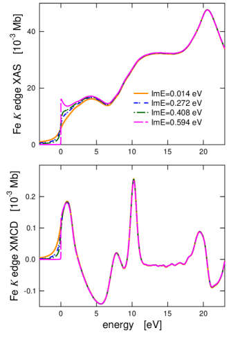
Figure 1: Fe $K$ edge XAS and XMCD calculated for different imaginary energies and convoluted subsequently with Lorentzians chosen so that the total spectral broadening $2\text{Im}E+\Gamma_{K}$ remains constant.

We start by inspecting how shifting the weight of the broadening from a Lorentzian convolution to an imaginary energy component affects the calculated XAS and XMCD. This is done in Fig. 1 for the Fe $K$ edge and in Fig. 2 for the Fe $L_{2,3}$ edge. We focus solely on the theoretical spectra; a good agreement of theory with experiment was demonstrated earlier.Šipr and Ebert (2005); Šipr et al. (2011)

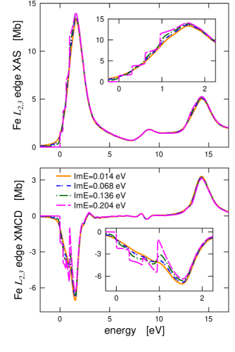
Figure 2: As Fig. 1 but for the $L_{2,3}$ edge. The insets show detailed views on the $L_{3}$ edge region.

One can see that for energies higher than about $5\,\Gamma_{\text{core}}$ above the edge there is practically no difference in the spectra, no matter which broadening procedure has been applied. At the very edge, however, there are differences. They stem from the fact that if too much weight is put on broadening by means of the imaginary energy component, there is a sharp cut-off of the spectra at $E_{F}$, resulting in too sharp features at the edge. If a sufficient amount of broadening is done via Lorentzian convolution, this cut-off is smeared out.

The situation is especially instructive for the Fe $L_{3}$ edge XMCD peak. Here a well-distinguished but in fact spurious fine structure appears on its low-energy side unless most of the broadening is done by means of Lorentzian convolution. The situation is much less dramatic for the corresponding XAS peak. This is because of the way the XMCD peak is generated: it is a sum of four ($L_{3}$ edge) or two ($L_{2}$ edge) contributions which may have opposite signs and which have their edges at slightly different energies due to the relativistic exchange splitting of the core levels.

III.2 ($\kappa$,$\mu$)-resolved spectra

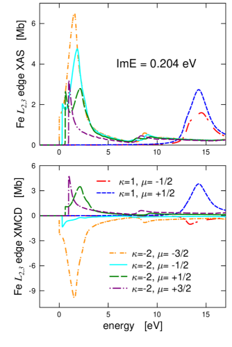
Figure 3: ($\kappa$,$\mu$)-decomposed Fe $L_{2,3}$ edge XAS and XMCD calculated for imaginary energy 0.204 eV and convoluted subsequently with Lorentzians of $\Gamma_{L_{2}}=0.732$ eV (for the $L_{2}$ edge) and $\Gamma_{L_{3}}=0.002$ eV (for the $L_{3}$ edge).

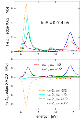
Figure 4: As Fig. 3 but for for imaginary energy 0.014 eV and Lorentzian widths $\Gamma_{L_{2}}=1.113$ eV and $\Gamma_{L_{3}}=0.383$ eV for the $L_{2}$ and $L_{3}$ edges, respectively.

An insight can be obtained by looking at individual ($\kappa$,$\mu$)-components contributing to the Fe $L_{2,3}$ edge XAS and XMCD for the two extreme cases, with $\text{Im}E=0.204$ eV (nearly all broadening done via the imaginary energy component) and with $\text{Im}E=0.014$ eV (nearly all broadening done via a convolution with a Lorentzian — cf. Tab. 2). If one looks at the spectra obtained using $\text{Im}E=0.204$ eV (Fig. 3), one can see that the individual components indeed exhibit sharp edges or onsets at different energies. If all components have the same sign, as is the case of XAS, the resulting spectrum is “rugged” but in general not so much different from the spectra obtained for smaller $\text{Im}E$ (see the upper panel in Fig. 2). However, if the individual ($\kappa$,$\mu$) components differ in signs as in the case of XMCD, their sum may give rise to a spectrum which is significantly different from the spectrum obtained for smaller $\text{Im}E$ (the lower panel in Fig. 2). Technically, this difference can be understood by comparing Fig. 3 with Fig. 4, which is its analog but with a smaller imaginary energy part $\text{Im}E=0.014$ eV. One case see that if the individual ($\kappa$,$\mu$)-components have been smoothed before the summation, the resulting spectrum is smooth as well, without the quasi-oscillation at about 1 eV which appears in the XMCD spectrum for larger $\text{Im}E$’s (cf. Fig. 2).

IV Discussion

Our aim was to check whether employment of complex energies for calculating broadened XAS and XMCD spectra can introduce significant distortions in comparison with what is obtained by convoluting the spectra calculated on the real axis. Our results indicate that simulating the finite core hole lifetime by means of an imaginary energy component and by means of convoluting the raw spectra with a Lorentzian is equivalent only for energies higher than few core level FWHM’s above the absorption edge. If too much weight is put on broadening via an imaginary energy component, spurious spectral features may appear close to the edge, especially for the dichroic spectra.

When contemplating practical implications of this, one should realize that there are other sources of spectral broadening that we did not consider. In particular the finite lifetime of the photoelectronMüller et al. (1982) and also atomic vibrations.Beni and Platzman (1976); Fujikawa et al. (1999); Šipr et al. (2016) The influence of these effects will be, nevertheless, small at the very edge, which is the region where there is the largest likelihood that the ansatz Eq. (4) will be inappropriate. Another factor important for comparison with experiment is the instrumental broadening. This is usually accounted for by a Gaussian smearing. Typical values for the width of the Gaussian are 0.8 eV for the Fe $K$ edge and 0.2 eV for the Fe $L_{2,3}$ edge. Applying the instrumental broadening would thus remove most of the significant differences between individual spectra shown in Fig. 1 and also between the XAS spectra shown in the upper panel of Fig. 2. However, the spurious fine structure appearing for large $\text{Im}E$’s at the low-energy side of the Fe $L_{3}$ edge XMCD peak would remain.

Typical values of the imaginary energy component used for XAS/XMCD calculations are $\text{Im}E\sim 0.1$–0.2 eV. It follows from our results that while this is appropriate for most situations, problems might occur for edges where the core hole lifetime broadening is small — such as the $L_{3}$ edges of 3$d$ transition metals. Special care should be taken for XMCD spectra: it is still reasonable to perform the calculations for complex energies to reduce the computing workload but $\text{Im}E$ should be smaller than usually. To give a specific recommendation, we suggest that $\text{Im}E$ should be about one tenth of the tabulated FWHM value, i.e., 0.1$\times\Gamma_{\text{core}}$. An energy mesh dense enough to account for all fine features that might be present in the spectrum should have a step of $\text{Im}E$/2.

The severity of the effect investigated here increases if the applied core hole lifetime broadening $\Gamma_{\text{core}}$ decreases. For example, if we had used FWHM’s recommended by an older compilation of Al Shamma et al.Shamma et al. (1992) which are about 50 % less than the values recommended by the newer compilation of Campbell and Papp,Campbell and Papp (2001) the spurious fine structure at the Fe $L_{3}$ edge XMCD peak would be even more pronounced. On the other hand, the fact that core hole lifetime widths are usually not known very accurately means that the effect explored here may be overlooked: if redundant structures appear close to the edge, one might be tempted to apply mechanically additional broadening, without considering that one may be actually dealing with an artefact caused by the mechanism analyzed here.

Finally, the fact that both ways of dealing with core hole lifetime broadening are equivalent sufficiently high above the edge justifies formally the use of exponential damping in the EXAFS region.Lee et al. (1981) Namely, it can be shown that if the free-electron Green’s function is evaluated for a complex energy

$$E\>+\>\mathrm{i}\,\Gamma/2\quad,$$

it gives rise to exponential damping of the photoelectron probability with the mean free path $\lambda$,Müller et al. (1982); Natoli et al. (2003); Sébilleau et al. (2006)

$$\lambda\>=\>\frac{\hbar}{\Gamma}\,\sqrt{\frac{2E}{m}}\quad.$$

This leads straightforwardly to the $\exp(-R/\lambda)$ factor used in the EXAFS formula.Lee et al. (1981); Natoli et al. (2003) One only has to take care whether the mean free path $\lambda$ is related to the photoelectron probability as it is the case here or whether it is related to the amplitude [then the proper factor is $\exp(-2R/\lambda)$].

V Conclusions

Well above the absorption edge, the two ways of incorporating the finite core hole lifetime into calculation of x-ray absorption spectra, namely, via adding an imaginary component to the energy and via convoluting the raw spectrum with a Lorentzian, are equivalent. However, this is not the case close to the edge. Ignoring this can lead to emergence of spurious spectral features. Special care should be taken for dichroic spectra at edges which comprise several exchange-split core levels, as is the case of the $L_{3}$ edge of 3$d$ transition metals.