Arbitrage and Geometry

1 Introduction

Arbitrage is the financial world’s tooth fairy. Just as the tooth fairy provides a guaranteed financial return for baby teeth, an arbitrage opportunity is an investment, or combination of investments, that is guaranteed to yield a profit. Arbitrage shares another important property with the tooth fairy: neither of them exist. The “no free lunch” assumption, that arbitrage opportunities in the marketplace are unavailable, has played a fundamental role in financial economics. In 1958, Modigliani and Miller [MM58] used the principle to argue that the way a company finances itself, either by use of bonds or by issuing additional stock is irrelevant in determining its value. The principle appears in the options pricing formula due to Merton, Black, and Scholes [BS73, Mer73]. The principle was placed on a solid theoretical footing in the work of Ross [Ros76a, Ros76b]. A gentle introduction to the arbitrage principle is [Var87].

This article introduces the notion of arbitrage for a situation involving a collection of investments and a payoff matrix describing the return to an investor of each investment under each of a set of possible scenarios. We explain the Arbitrage Theorem, discuss its geometric meaning, and show its equivalence to Farkas’ Lemma. We then ask a seemingly innocent question: given a random payoff matrix, what is the probability of an arbitrage opportunity? This question leads to some interesting geometry involving hyperplane arrangements and related topics.

1.1 Payoff matrices.

A dizzying array of investment opportunities is available to someone who has money to invest. There are stocks, bonds, commodities, foreign currency, stock options, futures, real estate, and of course, savings accounts. We make the simplifying assumption that there are $n$ possible choices of investments available, and that at this moment of time (today) one may invest any amount of one’s finances in each. At the end of a fixed time period (tomorrow), a single unit of cash (a dollar, a euro, a yen, etc.) invested in investment $i$ will be worth some amount of money, so that changes in value of the investments can be represented as an $n$-dimensional vector. A further simplifying assumption is that there are finitely many mutually exclusive scenarios that can occur, and that each scenario leads to a specific gain (or loss) for each investment.

As a consequence of these assumptions, we represent the changes in value, or returns, be they gains or losses, in an $m\times n$ payoff matrix This is a matrix with a row corresponding to each scenario and a column corresponding to each investment. The $j,i$ entry, $a_{ji},$ gives the change in value at the end of the time period based on a unit invested in investment $i$ under scenario $j$. See Figure 1. Entries in this matrix are positive if the investment gains value and negative if it loses value.

1.2 Risk-free Rate.

It is typical to assume that there is a risk-free investment (e.g. U.S. Treasury Bills) available to the investor that yields a payoff tomorrow of $1+r$ units for each unit invested. Thus, a single unit today is guaranteed to be worth $1+r$ units tomorrow. We express gains or losses tomorrow in present day units, by multiplying by a discount factor of $1/(1+r).$

Thus, if we invest one unit of cash today in an investment and it becomes worth $x$ units tomorrow, the relevant entry in the payoff matrix is its present value $-1+x/(1+r)$.

$$\begin{array}[]{c|ccccccc}&I_{1}&I_{2}&\cdots&I_{i}&\cdots&I_{n}\\ \hline\cr\mbox{Scenario}_{1}&a_{11}&a_{12}&\cdots&a_{1i}&\cdots&a_{1n}\\ \mbox{Scenario}_{2}&a_{21}&a_{22}&\cdots&a_{2i}&\cdots&a_{2n}\\ \vdots&\vdots&\vdots&&\vdots&&\vdots\\ \mbox{Scenario}_{j}&a_{j1}&a_{j2}&\cdots&a_{ji}&\cdots&a_{jn}\\ \vdots&\vdots&\vdots&&\vdots&&\vdots\\ \mbox{Scenario}_{m}&a_{m1}&a_{m2}&\cdots&a_{mi}&\cdots&a_{mn}\\ \end{array}$$

Figure 1: The $j,i$ entry of payoff matrix $A$ is the gain (or loss) tomorrow under scenario $j$ for a unit invested in investment $i$ today.

1.3 Example: The Bernoulli model

The following simple example is a standard one that appears in most introductory books on options pricing, and is included here to give the reader a taste for how options are priced. Assume that when we invest one unit in a certain stock today, currently priced at $S$, its value tomorrow either be one of two possibilities, either $Su$ or $Sd$, where $d<1+r<u$, so that the stock under- or over-performs the risk-free rate. Consequently, there are two possible payoffs tomorrow of a single unit investment in the stock today, $u$ or $d$, and discounting gives either a value change of $-1+u/(1+r)$ or $-1+d/(1+r)$ in today’s terms.

Another possibility is to purchase a stock option referred to as a call: we pay someone an amount $P$ today for the right to buy from them a share of the stock at a predetermined price $K$ (called the strike price) tomorrow (no matter what happens to the market price), where $Sd<K<Su.$ If the stock goes up, then we would exercise our right to buy it at $K$ and then immediately sell it at the market price of $Su,$ instantly netting $Su-K.$ In this case, the net gain for buying the option (taking into account discounting) is

$$-P+(Su-K)/(1+r).$$

In other words, investing a single unit of money in such an option results in a value change of

$$-1+(Su-K)/(P(1+r)).$$

On the other hand, if the stock goes down we would not want to exercise the option since we would be better off purchasing the stock at the lower market price, and in this case we have simply lost the cost of the option.

Thus, we can write down a $2\times 2$ payoff matrix corresponding to the two investment opportunities (stock, option) and the two possible scenarios (stock goes up, stock goes down) as in Figure 2. A third column representing the payoff for a risk-free investment of one unit could be adjoined to this matrix. However, this column would consist of zeros, since discounting leaves the present value of such an investment unchanged.

$$\begin{array}[]{c|cc}&\mbox{stock}&\mbox{option}\\ \hline\cr\mbox{up}&-1+u/(1+r)&-1+(Su-K)/(P(1+r))\\ \mbox{down}&-1+d/(1+r)&-1\\ \end{array}$$

Figure 2: The payoff matrix for a stock whose price today is $S$ and whose price tomorrow takes one of two values $Su$ or $Sd$, and for an option whose price today is $P$ and gives one the right to purchase the stock at a strike price of $K$ tomorrow. The risk-free interest rate for this one day period is $r$.

1.4 Arbitrage

In finance, an arbitrage opportunity is a combination of investments whose return is guaranteed to outperform the risk-free rate. If such an opportunity were to exist we could borrow money at the lower rate, get the higher return, repay our debt, and pocket the difference. Since our initial investment is unlimited, so is the amount of money we could make. In modeling the behavior of markets, a common approach is to assume that an equilibrium condition exists under which such opportunities are not available; if they were to become available, they could only exist for an extremely brief period of time. Almost as soon as they are discovered, they are wiped out as a result of the response of investors.

The no arbitrage assumption is as fundamental a principle for finance as Newton’s first and second laws of motion are for physics. Another important principle bears semantic resemblance to Newton’s third law: for every action there is an equal and opposite reaction. In finance, everything that can be bought can also be sold.

A consequence of this is that for every available payoff column there is an investment opportunity that achieves exactly the opposite effect, that is, changes the signs of the payoffs. This may seem counterintuitive. For example, what investment leads to a payoff that is complementary to the purchase of a share of stock? The answer is to short sell it, that is, in essence, borrow it, sell it, and later buy it back and subsequently return it to the lender. Consequently, a column in the payoff matrix may be replaced by any nonzero multiple of the column, and the modified matrix represents the same investment opportunities.

Given a specific payoff matrix $A$ that gives the behavior of all possible investments and scenarios, an arbitrage opportunity is said to exist if there is a linear combination of columns of $A$ all of whose entries are strictly positive. Thus, an arbitrage opportunity is a combination of buys and sells of the basic investments that yields a net gain under all scenarios.

The absence-of-arbitrage assumption leads to constraints on payoff matrices. To illustrate this, consider the stock/option example above. If the two columns of the matrix in Figure 2 are not scalar multiples of each other, then they form a basis of $\mathbb{R}^{2}$ and so we can find a combination of buys and sells of the two investments to yield any payoff vector we wish. Thus, the absence of arbitrage implies that the two columns are multiples of each other, and this gives

$$P=\frac{(Su-K)(1+r-d)}{(1+r)(u-d)},$$

so that once the various parameters involved, including the interest rate, the possible factors by which the stock price can change, the price of the stock today, and the strike price $K,$ are set, the price of the option can be calculated.

2 The Arbitrage Theorem

The Arbitrage Theorem provides an interesting and convenient characterization of the no arbitrage condition. Given an $m\times n$ payoff matrix $A,$ and an $n$-vector $x$, the product $Ax$ gives the payoff vector that results from investing $x_{i}$ in investment $i,$ for $i=1,\ldots,n.$ Consequently, for a given payoff matrix $A,$ its column space colspace(A), represents the set of payoff vectors corresponding to all possible combinations of investments. This forms a subspace of $\mathbb{R}^{m}$ of dimension at most $n$.

Theorem 1 (Arbitrage).

Given an $m\times n$ payoff matrix $A$, exactly one of the following statements holds:

• Some payoff vector in $\mbox{colspace}(A)$ has all positive components, i.e. $Av>0$ for some $v\in\mathbb{R}^{n}.$

• There exists a probability vector $\pi=[\pi_{1},\ldots,\pi_{m}]^{t}$ that is orthogonal to every column of $A,$ i.e. $\pi^{t}A=0,$ where $\pi^{t}\geq 0$ and $\pi^{t}1=1.$

In other words, the absence of arbitrage is equivalent to the existence of an assignment of probabilities to scenarios under which every investment has an expected return of zero.

For a concrete example, consider the situation described above in which our payoff matrix contains a column of the form

$$\left[\begin{array}[]{cc}-1+u/(1+r)\\ -1+d/(1+r)\\ \end{array}\right].$$

The absence of arbitrage means that there is a probability vector

$$\left[\begin{array}[]{cc}\pi_{u}\\ \pi_{d}\\ \end{array}\right]$$

orthogonal to it and every other column of the payoff matrix. It follows immediately that $\pi_{u}=\frac{1+r-d}{u-d}$ and $\pi_{d}=1-\pi_{u}=\frac{u-1-r}{u-d}$.

These probabilities do not have the familiar interpretation as relative frequencies. However, the probability assignment is a practical one in that under the assumption of no arbitrage, any investment should have a zero expected payoff. Thus, these probabilities provide us with a method for establishing the price of any security whose payoff depends on the behavior of the stock. For example, suppose we have the opportunity to invest in a security whose price is $P$ today and whose payoff tomorrow is $\rho_{u}$ if the stock goes up and $\rho_{d}$ if the stock goes down. Then we can add a column to our payoff matrix describing the present value corresponding to a unit investment

$$\left[\begin{array}[]{cc}-1+\rho_{u}/P(1+r)\\ -1+\rho_{d}/P(1+r).\\ \end{array}\right].$$

Absence of arbitrage leads to the conclusion that

$$\pi_{u}\left(-1+\rho_{u}/P(1+r)\right)+\pi_{d}\left(-1+\rho_{d}/P(1+r)\right)=0,$$

and solving for $P$ we obtain

$$P=\pi_{u}\rho_{u}/(1+r)+\pi_{d}\rho_{d}/(1+r),$$

that is, the no-arbitrage price of the investment is the expected value of its discounted payoff.

The Arbitrage Theorem (also known as Gordon’s Theorem) is but one example of a theorem of the alternative appearing in convex analysis in which one asserts the existence of a vector satisfying exactly one of two properties. One of the more fundamental results of this type is Farkas’ Lemma [Far02], treatments of which may be found in many books on finite-dimensional optimization, including [BT97, Pad99, SW70] (see also [AK04]). The Arbitrage Theorem is frequently presented as a simple consequence of Farkas’ Lemma, for example, see [BT97, Ros02]. A lengthy treatment of theorems of the alternative appears in [Man94], together with a table (Table 2.4.1) of eleven such theorems.

Lemma 2 (Farkas).

Given an $m\times n$ matrix $A$ and an $n$-vector $b,$ exactly one of the following statements holds:

• There exists $x\geq 0$ such that $Ax=b.$

• There exists $y$ such that $y^{t}A\geq 0$ and $y^{t}b<0.$

Equivalently, the following two statements are equivalent:

• There exists $x\geq 0$ such that $Ax=b.$

• $y^{t}A\geq 0$ implies $y^{t}b\geq 0.$

Definition 3.

The polyhedral convex cone generated by $a^{(i)}\in\mathbb{R}^{m},~{}i=1,\ldots,n$ is the subset of $\mathbb{R}^{m}$ defined by

$$\left\{\sum_{i=1}^{n}x_{i}a^{(i)}~{}:~{}x_{i}\geq 0\right\}.$$

We denote this set by $\mathcal{C}(a^{(i)},i=1,\ldots,n)$ and we refer to the $a^{(i)},~{}i=1,\ldots,n$ as generators of the cone.

Farkas’ Lemma has an intuitive geometric interpretation. Let the columns of $A$ be denoted by $a^{(i)},~{}i=1,\ldots,n,$ and take

$$\mathcal{C}_{A}:=\mathcal{C}(a^{(i)},i=1,\ldots,n).$$

Condition (F1) says that $b\in\mathcal{C}_{A}.$ On the other hand, assuming $b\neq 0,$ (F2) says that if $y$ makes a non-obtuse angle with every non-zero cone generator $a^{(i)}$ then the angle $y$ makes with $b$ is non-obtuse.

We show how the Arbitrage Theorem follows from Farkas’ Lemma and, conversely, how to prove Farkas’ Lemma from the Arbitrage Theorem. Farkas’ Lemma is central to the theory of linear programming and, in the same spirit, [Rei85] shows how various combinatorial duality theorems can be derived from one another.

2.1 Proof of the Arbitrage Theorem using Farkas’ Lemma

Proof.

First, if (A1) and (A2) are both satisfied, then we have

$$\pi^{t}Av=0v=0,$$

but on the other hand $Av>0$ so $\pi^{t}Av>0$ since the entries in $\pi$ are nonnegative and sum to one. It follows that (A1) and (A2) are mutually exclusive.

Next we show that (A1) and (A2) cannot both fail. If (A2) fails, then there is no solution to

$$\left[\begin{array}[]{c}A^{t}\\ 1\\ \end{array}\right]\pi=\left[\begin{array}[]{c}0\\ 1\\ \end{array}\right]$$

with $\pi\geq 0.$ It follows that condition (i) in Farkas’ Lemma fails for $\tilde{A}=\left[\begin{array}[]{c}A^{t}\\ 1\\ \end{array}\right]$ and $\tilde{b}=\left[\begin{array}[]{c}0\\ 1\\ \end{array}\right],$ so Farkas’ Lemma guarantees that (ii) holds. Therefore, there exists an $n+1$-vector $y$ such that $y^{t}\tilde{A}\geq 0$ and $y^{t}\tilde{b}<0.$ Writing $y=\left[\begin{array}[]{c}v\\ s\\ \end{array}\right]$ where $v=[v_{1},\ldots,v_{n}]^{t}$ and $s\in\mathbb{R}$ these conditions say that $Av+s1\geq 0$ and $s<0,$ and we conclude that $Av>0,$ so (A1) is valid. ∎

2.2 Proving Farkas’s Lemma from the Arbitrage Theorem

As it turns out, the Arbitrage Theorem together, with some work, leads to a proof of Farkas’ Lemma. Note first that the implication (F1) $\Rightarrow$ (F2) is immediate: if we can find $x\geq 0$ such that $Ax=b,$ then assuming that $y^{t}A\geq 0$ we have $y^{t}b=y^{t}Ax\geq 0.$

Our focus is on the more difficult implication (F2) $\Rightarrow$ (F1). It is instructive to first prove this under a certain technical assumption. For a polyhedral convex cone $\mathcal{C}\subseteq\mathbb{R}^{m},$ we define

$$\mathcal{L}(\mathcal{C}):=\mathcal{C}\cap-\mathcal{C}.$$

This is easily seen to form a subspace of $\mathbb{R}^{m}$ and consists of all lines completely contained in $\mathcal{C}$ passing through the origin.

Definition 4.

A polyhedral convex cone $\mathcal{C}$ is pointed if $\mathcal{L}(\mathcal{C})=\{0\}.$ In other words, if it contains no lines through the origin, that is, $v,-v\in\mathcal{C}$ implies $v=0.$

The reader is referred to Figures 3 and 4.

Figure 3: The vectors $a^{(i)},i=1,2,3$ generate a pointed cone in $\mathbb{R}^{3}.$

Figure 4: The vectors $a^{(i)},i=1,2,3,4$ generate a non-pointed cone in $\mathbb{R}^{3}.$

It is an elementary exercise to prove that pointedness for the cone $\mathcal{C}_{A}$ says that whenever $\sum_{i=1}^{n}x_{i}a^{(i)}=0$ for $x_{i}\geq 0,~{}i=1,\ldots,n$ we can conclude that $x_{i}a^{(i)}=0$ for all $i.$

Lemma 5.

The implication (F2) $\Rightarrow$ (F1) holds when $A$ is an $m\times n$ matrix such that $\mathcal{C}_{A}$ is a pointed cone.

Proof.

Observe that (F2) holds for a matrix $A,$ then it also holds for the matrix obtained by removing any zero columns of $A.$ Also, if (F1) holds for the matrix with the zero columns of $A$ removed then it also holds for the original matrix. It follows that, without loss of generality, we may assume that all of the columns of $A$ are nonzero.

It follows from (F2) that

$$\left[\begin{array}[]{c}A^{t}\\ -b^{t}\end{array}\right]y\not>0,$$

for all $y.$ Thus, condition (A1) fails, and from the Arbitrage Theorem we conclude that (A2) holds, that is, there exists a probability vector $\left[\begin{array}[]{c}u\\ s\end{array}\right]$ with $u$ an $n$-vector, and $s$ a scalar, such that

$$[u^{t},s]\left[\begin{array}[]{c}A^{t}\\ -b^{t}\end{array}\right]=0.$$

Expanding and transposing, we obtain $Au=sb.$ We can assume $s>0$ since otherwise the assumption of pointedness is violated. It follows that we can divide both sides by $s$ and we obtain (F1). ∎

To establish the general case we need to collect some basic results concerning the structure of non-pointed polyhedral convex cones. The basic idea is that one can always represent a cone as a direct sum of a linear subspace and a pointed slice of the cone (see Figure 5). The proof is left as an elementary exercise.

Lemma 6.

Given a polyhedral convex cone $\mathcal{C}=\mathcal{C}(a^{(i)},i=1,\ldots,n)\subseteq\mathbb{R}^{m},$ let $\mathcal{L}=\mathcal{L}(\mathcal{C})$ and let $\mathcal{L}^{\perp}$ denote its orthogonal complement. Then any given $x\in\mathcal{C}$ can be expressed uniquely as $x=u+v$ where $u\in\mathcal{C}\cap\mathcal{L}^{\perp},$ $v\in\mathcal{L}.$ We express this statement symbolically by writing

$$\mathcal{C}=(\mathcal{C}\cap\mathcal{L}^{\perp})\oplus\mathcal{L}.$$

Furthermore, if $\tilde{a}^{(i)}$ denotes the orthogonal projection of $a^{(i)}$ onto $\mathcal{L}^{\perp},$ for $i=1,\ldots,n,$ then

$$\mathcal{C}\cap\mathcal{L}^{\perp}=\mathcal{C}(\tilde{a}^{(i)},i=1,\ldots,n),$$

and the slice $\mathcal{C}\cap\mathcal{L}^{\perp}$ is a pointed polyhedral convex cone.

Figure 5: Slicing the cone in Figure 4 yields a pointed cone.

Armed with these results we are now prepared to use the Arbitrage Theorem to show (F2) $\Rightarrow$ (F1).

Proof of Farkas’ Lemma by way of the Arbitrage Theorem.

Assume (F2) holds for a given $m\times n$ matrix $A$ with columns $a^{(i)},i=1,\ldots,n.$ Take $\mathcal{C}=\mathcal{C}(a^{(i)},i=1,\ldots,n)$, $\mathcal{L}=\mathcal{L}(\mathcal{C}),$ $\mathcal{L}^{\perp},$ and $\tilde{a}^{(i)}$ to be the orthogonal projection of $a^{(i)})$ on $\mathcal{L}^{\perp},$ for $i=1,\ldots,n.$ We can write $a^{(i)}=\tilde{a}^{(i)}+\hat{a}^{(i)},$ and where $\hat{a}^{(i)}\in\mathcal{L}.$ Also, we define $\tilde{b}$ to be the orthogonal projection of $b$ onto $\mathcal{L}^{\perp}$ and we write $b=\tilde{b}+\hat{b},$ where $\hat{b}\in\mathcal{L}.$

Now suppose $y\in\mathcal{L}^{\perp}\subseteq\mathbb{R}^{m}$ and $y^{t}\tilde{a}^{(i)}\geq 0$ for $i=1,\ldots,n.$ Then $y^{t}a^{(i)}=y^{t}\tilde{a}^{(i)}+y^{t}\hat{a}^{(i)}=y^{t}\tilde{a}^{(i)}\geq 0,$ for $i=1,\ldots,n$ and we can conclude from (F2) that $y^{t}b\geq 0.$ It follows that $y^{t}\tilde{b}=y^{t}(b-\hat{b})=y^{t}b\geq 0.$

Summarizing, we have shown that

$$y\in\mathcal{L}^{\perp}\subseteq\mathbb{R}^{m}\text{ and }y^{t}\tilde{a}^{(i)}\geq 0\text{ for }i=1,\ldots,n\quad\Rightarrow\quad y^{t}\tilde{b}\geq 0.$$

Since the $\tilde{a}^{(i)},i=1,\ldots,n$ generate a pointed cone in $\mathcal{L}^{\perp}$ and $\tilde{b}\in\mathcal{L}^{\perp},$ Lemma 6 allows us to conclude that $\tilde{b}\in\mathcal{C}(\tilde{a}^{(i)},i=1,\ldots,n),$ i.e. we can write $\tilde{b}=\sum_{i=1}^{n}x_{i}\tilde{a}^{(i)}$ for some $x_{i}\geq 0.$ It follows that

$$b=\tilde{b}+\hat{b}=\sum_{i=1}^{n}x_{i}\tilde{a}^{(i)}+\hat{b}=\sum_{i=1}^{n}x_{i}(a^{(i)}+\hat{a}^{(i)})+\hat{b}=\sum_{i=1}^{n}x_{i}a^{(i)}+\left\{\sum_{i=1}^{n}x_{i}\hat{a}^{(i)}+\hat{b}\right\}\in\mathcal{C},$$

where we have used the fact that $\mathcal{L}\subseteq\mathcal{C}$ to conclude that the term in braces lies in $\mathcal{C}.$ ∎

3 Geometry of generic payoff matrices

For a given $m\times n$ payoff matrix, the existence of arbitrage amounts to the statement that $\mbox{colspace}(A)$ intersects the positive orthant $\mathcal{O}^{+}:=\left\{x\in\mathbb{R}^{m}:x_{j}>0,~{}j=1,\ldots,m\right\}.$ Thus the probability that a random payoff matrix exhibits arbitrage equals the probability that its column space meets the positive orthant which, in turn, is the probability that a random $n$-dimensional subspace of $\mathbb{R}^{m}$ intersects $\mathcal{O}^{+}$.

This leads us to ask: How many orthants does an $n$-dimensional subspace of $\mathbb{R}^{m}$ intersect? For the most part, the answer is independent of the choice of the subspace and is closely related to other geometric counting problems. See [Buc43] in particular, but also [AS00], [Bru99] pages 285–290, [Com74] page 73, [Jam43], [MS82], [OT92], [Wei], [Woo43], [Zas85], and [Zas75].

Let $e_{1},e_{2},\ldots,e_{m}$ denote the standard orthonormal basis of $\mathbb{R}^{m}$.

Definition 7.

Let $\mathcal{V}$ be an $n$-dimensional subspace of $\mathbb{R}^{m}$. We say that $\mathcal{V}$ is generic if for some (and therefore for any) basis $\{v_{1},v_{2},\ldots,v_{n}\}$ of $\mathcal{V}$ and for any $m-n$ standard basis vectors $e_{i_{1}},\ldots,e_{i_{m-n}}$, the vectors $\{v_{1},v_{2},\ldots,v_{n},e_{i_{1}},\ldots,e_{i_{m-n}}\}$ are linearly independent. Likewise, an $m\times n$ matrix $A$ is called generic if $\mbox{colspace}(A)$ is a generic subspace of $\mathbb{R}^{m}$.

Next we present some notation for the orthants of $\mathbb{R}^{m}$. Let $\Pi_{j}=e_{j}^{\perp}$. The subspaces $\Pi_{j}$ are the coordinate hyperplanes and these separate $\mathbb{R}^{m}$ into orthants, i.e., the connected components of $\mathbb{R}^{m}-\bigcup\Pi_{j}$. Two vectors $v$ and $w$ (none of whose coordinates is zero) are in the same orthant provided the sign of $v_{i}$ equals the sign of $w_{i}$ for all $i$.

Denote by $\mathcal{S}_{m}$ the set of $m$-vectors $\delta=(\delta_{1},\ldots,\delta_{m})$ where each $\delta_{i}$ is $\pm 1$. Multiplication of members of $\mathcal{S}_{m}$ is defined coordinatewise. The orthant $\mathcal{O}_{\delta}$ is defined by

$$\mathcal{O}_{\delta}=\{x\in\mathbb{R}^{m}:\delta_{i}x_{i}>0,~{}i=1,\ldots,m\}.$$

The positive orthant $\mathcal{O}^{+}$ is simply $\mathcal{O}_{(1,1,\ldots,1)}$.

A generic subspace $\mathcal{V}$ of $\mathbb{R}^{m}$ intersects some subset of the orthants of $\mathbb{R}^{m}$. Two points in $\mathcal{V}$ lie in different orthants of $\mathbb{R}^{m}$ exactly when they are separated by some coordinate hyperplane(s) $\Pi_{j}$. Thus, there is a one-to-one correspondence between the orthants intersected by $\mathcal{V}$ and the connected components of

$$\mathcal{V}-\bigcup_{j=1}^{m}\Pi_{j}.$$

The intersections of $\mathcal{V}$ with the coordinate hyperplanes $\Pi_{j}$ are subspaces of $\mathcal{V}$ with particular properties; we show that they have codimension $1$ (i.e., have dimension $n-1$) and lie in general position.

Definition 8.

Subspaces $H_{1},\ldots,H_{m}$ of codimension 1 in an $n$-dimensional vector space are said to be in general position provided that $\dim\left(\bigcap_{j\in J}H_{j}\right)=n-|J|$ for all $J\subseteq\{1,\ldots,m\}$ with $1\leq|J|\leq n.$

For example, when $n=2$, any collection of distinct lines through the origin are in general position. When $n=3$, a collection of distinct planes through the origin are in general position provided no three of them intersect in a line.

For a subspace $H$ of codimension 1 in a vector space $\mathcal{V}$, the complement $\mathcal{V}-H$ consists of a pair of half-spaces that we can label arbitrarily as $H^{+}$ and $H^{-}.$

Given $m$ subspaces $H_{1},\ldots,H_{m}$ of codimension 1 whose associated half-spaces have been labeled, we can assign to every point in the complement $\mathcal{V}-\bigcup_{i=1}^{m}H_{i}$ an $m$-vector $\delta(x)=(\delta_{1}(x),\ldots,\delta_{m}(x))$ of signs, where the $\delta_{i}(x)$ indicates which half-space, $H_{i}^{+}$ or $H_{i}^{-},$ $x$ lies in. For each sign vector $\delta\in\mathcal{S}_{m}$ the set $\bigcap_{i=1}^{m}\left\{x\in\mathcal{V}~{}:~{}x\in H_{i}^{\delta_{i}}\right\}$ is an intersection of open half-spaces, so it is either empty or it is the interior of a convex polyhedron. Thus, the $H_{1},\ldots,H_{m}$ decompose $\mathcal{V}-\bigcup_{i=1}^{m}H_{i}$ into connected components, each associated with some $\delta\in\mathcal{S}_{m}$, which we refer to as cells.

Lemma 9.

Let $A$ be a generic $m\times n$ matrix and define $H_{i}=\mbox{colspace}(A)\cap\Pi_{i}$ for $i=1,\ldots,m.$ Then $H_{1},\ldots,H_{m}$ are subspaces of codimension $1$ in general position in $\mbox{colspace}(A).$ Furthermore, the connected components of $\mbox{colspace}(A)-\bigcup_{i=1}^{m}H_{i}$ correspond to the orthants that $\mbox{colspace}(A)$ intersects.

Proof.

Let $k=\dim(\mbox{colspace}(A))$ and let $J\subseteq\{1,\ldots,m\}$ with $1\leq|J|\leq k,$ then $|J^{c}|\geq m-k$ so we can find distinct indices $i_{1},\ldots,i_{m-k}\in J^{c}.$ Thus

$$\bigcap_{j\in J}\Pi_{j}=\mbox{span}\{e_{i}~{}:~{}i\in J^{c}\}\supseteq\mbox{span}\{e_{i_{1}},\ldots,e_{i_{m-k}}\},$$

and consequently

$$\mbox{colspace}(A)+\bigcap_{j\in J}\Pi_{j}\supseteq\mbox{colspace}\left[A,e_{i_{1}},\ldots,e_{i_{m-k}}\right],$$

so that by the genericity assumption

$$\dim(\mbox{colspace}(A)+\bigcap_{j\in J}\Pi_{j})=k+m-k=m.$$

It follows that

$$\dim(\mbox{colspace}(A)\cap\bigcap_{j\in J}H_{j}) =\dim(\mbox{colspace}(A)\cap\bigcap_{j\in J}\Pi_{j})$$

$$=\dim(\mbox{colspace}(A))+\dim(\bigcap_{j\in J}\Pi_{j})-\dim(\mbox{colspace}(A)+\bigcap_{j\in J}\Pi_{j})$$

$$=k+(m-|J|)-m$$

$$=\dim(\mbox{colspace}(A))-|J|,$$

so the subspaces $\mbox{colspace}(A)\cap\Pi_{i}$ are subspaces in $\mbox{colspace}(A)$ in general position.

The second claim is elementary. ∎

Thus, the number of orthants intersected by a generic $n$-dimensional subspace of $\mathbb{R}^{m}$ equals the number of cells determined by $m$ general-position, codimension-$1$ subspaces of $\mathbb{R}^{n}$. Our next step is to show that this value is given by

$$Q(m,n):=2\left[\binom{m-1}{0}+\binom{m-1}{1}+\cdots+\binom{m-1}{n-1}\right].$$

Figure 6 provides a small table of $Q(m,n)$ values.

	$n$
$m$	1	2	3	4	5	6	7	8
1	2	2	2	2	2	2	2	2
2	2	4	4	4	4	4	4	4
3	2	6	8	8	8	8	8	8
4	2	8	14	16	16	16	16	16
5	2	10	22	30	32	32	32	32
6	2	12	32	52	62	64	64	64
7	2	14	44	84	114	126	128	128
8	2	16	58	128	198	240	254	256

Figure 6: A table of $Q(m,n)$ values.

Proposition 10.

For positive integers $m$ and $n$ we have

• $Q(m,1)=2$,

• $Q(m,2)=2m$,

• for $m\leq n$, $Q(m,n)=2^{m}$ and so, in particular, $Q(1,n)=2$, and

• for $m,n\geq 2$, $Q(m,n)=Q(m-1,n)+Q(m-1,n-1)$.

Proof.

Claims (i)–(iii) are elementary and (iv) is established by the following routine calculation:

$$Q(m-1,n)+Q(m-1,n-1) =2\sum_{j=0}^{n-1}\binom{m-2}{j}+2\sum_{j=0}^{n-2}\binom{m-2}{j}$$

$$=\binom{m-2}{0}+2\sum_{j=0}^{n-2}\left[\binom{m-2}{j+1}+\binom{m-2}{j}\right]$$

$$=2\binom{m-1}{0}+2\sum_{j=0}^{n-2}\binom{m-1}{j+1}$$

$$=2\sum_{j=0}^{n-1}\binom{m-1}{j}=Q(m,n).\qed$$

Lemma 11.

Given $m$ subspaces of codimension $1$ in general position in a vector space $\mathcal{V}$ of dimension $n$, the number of connected components of $\mathcal{V}-\bigcup_{i=1}^{m}H_{i}$ depends only on $n$ and $m$ and is given by $Q(m,n)$.

For example, see Figure 7.

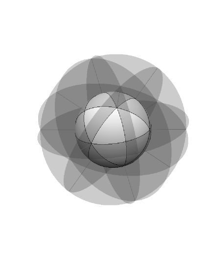
Figure 7: Slicing $\mathbb{R}^{3}$ with $4$ codimension-1, general-position subspaces gives $Q(4,3)=14$ regions.

Proof.

The result is easy to verify in case $m=1$ and in cases $n=1,2$, so we may assume $m,n\geq 2$.

It suffices, therefore, to show that the number of connected components satisfies the recursion formula in Proposition 10. We make the inductive assumption that the claim in the Lemma holds for $m-1$ subspaces (any $n$).

Consider $m$ general-position, codimension-1 subspaces $\mathcal{V}_{1},\mathcal{V}_{2},\ldots,\mathcal{V}_{m}$ of $\mathcal{V}$. By induction, the first $m-1$ of these cut $\mathcal{V}$ into $Q(m-1,n)$ regions.

Now consider the intersection of $\mathcal{V}_{1},\ldots,\mathcal{V}_{m-1}$ with $\mathcal{V}_{m}$. Let $\tilde{\mathcal{V}}_{i}=\mathcal{V}_{i}\cap\mathcal{V}_{m}$. Note that $\tilde{\mathcal{V}}_{1},\ldots,\tilde{\mathcal{V}}_{m-1}$ are codimension-1, general-position subspaces of $\mathcal{V}_{m}$, and therefore divide $\mathcal{V}_{m}$ into $Q(m-1,n-1)$ regions.

So the first $m-1$ subspaces $\mathcal{V}_{i}$ divide $\mathcal{V}$ into $Q(m-1,n)$ regions and the addition of $\mathcal{V}_{m}$ subdivides $Q(m-1,n-1)$ of those previous regions, giving a total of

$$Q(m-1,n)+Q(m-1,n-1)=Q(m,n)$$

regions, as required. ∎

Lemma 11 and its proof are analogous to the following well-known geometry problem [Buc43]: Given $m$ hyperplanes (not necessarily subspaces) in general position in $\mathbb{R}^{n}$, the number of regions defined by these hyperplanes is

$$\binom{m}{0}+\binom{m}{1}+\cdots+\binom{m}{n}$$

which equals $\frac{1}{2}Q(m+1,n+1)$. We can show this connection directly by the following geometric argument.

Consider $m$ general-position hyperplanes in $\mathbb{R}^{n}$; these determine $r$ regions. Extend $\mathbb{R}^{n}$ to $\mathbb{RP}^{n}$ and consider this arrangement of hyperplanes as sitting in $\mathbb{RP}^{n}$. When we do this some of the regions “wrap” past infinity, so to maintain the same number of regions $r$, we add the hyperplane at infinity to the arrangement. See Figure 8. Recall that a point in $\mathbb{RP}^{n}$ corresponds to a line through the origin in $\mathbb{R}^{n+1}$ and a hyperplane in $\mathbb{RP}^{n}$ corresponds to a codimension-1 subspace of $\mathbb{R}^{n+1}$. Since the hyperplanes of the original arrangement in $\mathbb{R}^{n}$ (and $\mathbb{RP}^{n}$) are in general position, these are now general position subspaces of $\mathbb{R}^{n+1}$. Each region of the arrangement of $m+1$ hyperplanes in $\mathbb{RP}^{n}$ splits into two antipodal regions when viewed as subspaces of $\mathbb{R}^{n+1}$. Thus, the $r$ original regions yield $2r$ regions determined by $m+1$ codimension-1, general position subspaces of $\mathbb{R}^{n+1}$, and so $2r=Q(m+1,n+1)$.

Figure 8: Slicing the plane with three lines, or the projective plane with four lines, gives $\frac{1}{2}Q(4,3)=7$ regions.

The values $Q(m,n)$ have an additional geometric interpretation. For example, the third column of the table in Figure 6 is sequence A014206 of The On-Line Encyclopedia of Integer Sequences [Slo]; these numbers are the maximum number of regions determined by $n$ circles in the plane; see Figure 9.

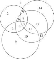
Figure 9: Four circles in the plane determine $Q(4,3)=14$ regions.

In general, the maximum number of regions determined by $m$ balls in $\mathbb{R}^{n-1}$ is $Q(m,n)$.

The various geometric interpretations of $Q(m,n)$ are collected in the following result.

Theorem 12.

Let $m,n$ be positive integers. Then $Q(m,n)$ equals all of the following:

1. $2\sum_{k=0}^{n-1}\binom{m-1}{k}$.

2. The number of regions defined by $m$ general-position, codimension-$1$ subspaces of $\mathbb{R}^{n}$.

3. The number of orthants intersected by a generic $n$-dimensional subspaces of $\mathbb{R}^{m}$.

4. The maximum number of regions determined by $m$ balls in $\mathbb{R}^{n-1}$.

5. Twice the number of regions determined by $m-1$ general-position hyperplanes in $\mathbb{R}^{n-1}$.

6. Twice the number of regions determined by $m$ general-position hyperplanes in $\mathbb{RP}^{n-1}$. ∎

Corollary 13.

Let $A$ be a generic $m\times n$ payoff matrix. Then the number of orthants that $\mbox{colspace}(A)$ intersects is $Q(m,n).$

Proof.

Since a generic payoff matrix is full-rank with $n\leq m$ the dimension of $\mbox{colspace}(A)$ is $n.$ By Lemma 9, $\mbox{colspace}(A)\cap\Pi_{1},\ldots,\mbox{colspace}(A)\cap\Pi_{m}$ are general-position, codimension-1 subspaces of $\mbox{colspace}(A)$, and the nonempty cells they define are in one-to-one correspondence with the orthants that $\mbox{colspace}(A)$ intersects. Using Lemma 11 the number of such cells is $Q(m,n).$ ∎

4 Random payoff matrices and the probability of arbitrage

Much of the research in mathematical finance is focused on modeling various markets and using these models to price various financial instruments. Our point of departure is to put aside entirely the consideration of real markets, and consider mathematically convenient random payoff matrices.

We ask: What is the probability that a random $m\times n$ payoff matrix admits an arbitrage opportunity? To make this question precise, one must give a probability distribution on matrices. However, for a wide range of natural probability distributions, the answer is $Q(m,n)/2^{m}$. Here’s the intuition. The $n$-dimensional column space of a random matrix $A$ intersects $Q(m,n)$ orthants. Since all orthants look the same, the probability that $\mbox{colspace}(A)$ intersects $\mathcal{O}^{+}$ is $Q(m,n)/2^{m}$. In other words, a ‘random’ $n$-dimensional subspace of $\mathbb{R}^{m}$ intersects $\mathcal{O}^{+}$ with probability $Q(m,n)/2^{m}$. (See [MS82] who consider random polytopes in $\mathbb{R}^{m}$.)

We now make this intuition precise.

We consider payoff matrices that are generic with probability one. This is not a difficult condition to attain as the next result makes clear.

Lemma 14.

Let $n\leq m$ and suppose $A$ be a random $m\times n$ payoff matrix whose entries have a continuous joint distribution. Then $A$ is generic with probability one.

Proof.

We identify $m\times n$ payoff matrices with points in $\mathbb{R}^{mn}$ in an obvious way, and the assumption says that for some function $f:\mathbb{R}^{mn}\rightarrow[0,+\infty)$ we have

$$P[A\in G]=\int_{G}f(x)dx$$

for $G\subseteq\mathbb{R}^{mn}.$ Genericity for $A$ fails if $\det[A,e_{i_{1}},\ldots,e_{i_{m-n}}]=0$ for some choice of distinct indices $i_{1},\ldots,i_{m-n}.$ Since there are only finitely many choices for such indices, we need only show that each set

$$\left\{A\in\mathbb{R}^{mn}~{}:~{}\det[A,e_{i_{1}},\ldots,e_{i_{m-n}}]=0\right\}$$

has Lebesgue measure 0. Since the determinant in this expression is a non-constant polynomial in the variables $A_{ij}$ the result follows. ∎

Corollary 15.

Let $n\leq m$ and suppose $A$ be a random $m\times n$ payoff matrix whose columns are iid random $m$-vectors whose distribution is continuous. Then $A$ is generic with probability one.

Observe that if $n\geq m$ and the entries of $A$ have a continuous joint distribution, then with probability one $\mbox{colspace}(A)=\mathbb{R}^{m},$ in which case $\mbox{colspace}(A)$ intersects every orthant, and in particular arbitrage occurs with with probability one. For this reason, it is more natural to focus on the case $n\leq m.$

Definition 16.

An $m\times n$ random payoff matrix is said to be invariant under reflections if its distribution is unaffected when any of its rows is multiplied by $-1.$

For example, if the $mn$ entries of $A$ are chosen independently from some probability distribution that is symmetric about $0$, then $A$ is invariant under reflections.

Given $\delta\in\mathcal{S}_{m}$ we let $R_{\delta}$ denote the $m\times m$ diagonal matrix whose diagonal is $\delta.$

Lemma 17.

Given an $m\times n$ payoff matrix $A,$ and $\delta,\omega\in\mathcal{S}_{m}$ we have $\mbox{colspace}(A)\cap\mathcal{O}_{\delta}\neq\emptyset$ if and only if $\mbox{colspace}(R_{\omega}A)\cap\mathcal{O}_{\omega\delta}\neq\emptyset.$

Proof.

This follows from the easy-to-verify fact that $Ax\in\mathcal{O}_{\delta}$ if and only $R_{\omega}Ax\in\mathcal{O}_{\omega\delta}$. ∎

Lemma 18.

If an $m\times n$ random payoff matrix $A$ is invariant under reflections then $\mbox{colspace}(A)$ intersects each of the $2^{m}$ orthants in $\mathbb{R}^{m}$ with equal probability.

Proof.

Given $\omega,\delta\in\mathcal{S}_{m},$ Lemma 17 gives

$$P\left[\mbox{colspace}(A)\cap\mathcal{O}_{\delta}\neq\emptyset\right]=P\left[\mbox{colspace}(R_{\omega}A)\cap\mathcal{O}_{\omega\delta}\neq\emptyset\right].$$

On the other hand, invariance under reflections guarantees that $R_{\omega}A$ has the same distribution as $A.$ Thus, this last probability equals

$$P\left[\mbox{colspace}(A)\cap\mathcal{O}_{\omega\delta}\neq\emptyset\right].$$

That is, $\mbox{colspace}(A)$ intersects $\mathcal{O}_{\delta}$ and $\mathcal{O}_{\omega\delta}$ with equal probability. Since $\omega\delta$ varies over all of $\mathcal{S}_{m}$ as $\omega$ varies over $\mathcal{S}_{m}$ the result follows. ∎

Our main result is the following.

Theorem 19.

If $A$ is a random $m\times n$ payoff matrix that is generic with probability one and invariant under reflections, then $\mbox{colspace}(A)$ intersects the orthant $\mathcal{O}_{\delta}$ with probability $Q(m,n)/2^{m}$ for any $\delta\in\mathcal{S}_{m}.$ In particular, such a matrix admits an arbitrage opportunity with probability $Q(m,n)/2^{m}$.

Proof.

Let $N(A)$ denote the number of orthants that $\mbox{colspace}(A)$ intersects. Since $A$ is generic with probability one, we apply Corollary 13 to conclude that $E\left[N(A)\right]=Q(m,n).$ On the other hand $N(A)$ is a sum of indicator random variables

$$N(A)=\sum_{\delta\in\mathcal{S}_{m}}I\left\{\mbox{colspace}(A)\cap\mathcal{O}_{\delta}\neq\emptyset\right\}$$

so that using Lemma 18

$$Q(m,n) =E\left[N(A)\right]$$

$$=\sum_{\delta\in\mathcal{S}_{m}}E\left[I\left\{\mbox{colspace}(A)\cap\mathcal{O}_{\delta}\neq\emptyset\right\}\right]$$

$$=\sum_{\delta\in\mathcal{S}_{m}}P\left[\mbox{colspace}(A)\cap\mathcal{O}_{\delta}\neq\emptyset\right]$$

$$=|\mathcal{S}_{m}|P\left[\mbox{colspace}(A)\cap\mathcal{O}^{+}\right]$$

$$=2^{m}P\left[\mbox{colspace}(A)\cap\mathcal{O}^{+}\right]$$

and the result follows. ∎

In particular, if $A$ is a random payoff matrix whose entries are independent and normally distributed with mean zero, then $A$ is generic with probability one and invariant under reflections.

Corollary 20.

Let $n$ be a positive integer. If $A$ is a random payoff matrix satisfying the conditions of Theorem 19 with $n$ columns (investments) and $2n$ rows (scenarios) then the probability of arbitrage is $1/2.$

For large random payoff matrices satisfying the conditions of the theorem we can use the central limit approximation [Fel68] to calculate the probability of an arbitrage.

Corollary 21.

Let $p(m,n)$ denote the probability of an arbitrage for an $m\times n$ random normal payoff matrix. If $n_{m}$ is a sequence such that

$$\lim_{m\rightarrow\infty}\frac{n_{m}-(m-1)/2}{\sqrt{(m-1)/4}}=x\in(-\infty,\infty)$$

then

$$\lim_{m\rightarrow\infty}p(m,n_{m})=\Phi(x),$$

where $\Phi$ denotes the standard normal cumulative distribution function.

References

- [AK04] D. Avis and B. Kaluzny. Solving inequalities and proving Farkas’s lemma made easy. This Monthly, 11:152–157, 2004.
- [AS00] P. K. Agarwal and M. Sharir. Arrangements and their applications. In J.-R. Sack and J. Urrutia, editors, Handbook of Computational Geometry, pages 49–119. North Holland, 2000.
- [Bru99] Richard A. Brualdi. Introductory Combinatorics. Prentice-Hall, third edition, 1999.
- [BS73] F. Black and M. J. Scholes. The pricing of options and corporate liabilities. Journal of Poliical Economy, 81:637–654, 1973.
- [BT97] D. Bertsimas and J.N. Tsitsiklis. Introduction to Linear Optimization. Athena Scientific, 1997.
- [Buc43] R. C. Buck. Partition of space. American Mathematical Monthly, 50(9):541–544, November 1943.
- [Com74] Louis Comet. Advanced Combinatorics: The Art of Finite and Infinite Expansions. D. Reidel, 1974.
- [Far02] J. Farkas. Theorie der einfachen ungleichungen. Journal für dir reine und angewandte Mathematik, 124:1–27, 1902.
- [Fel68] W. Feller. An Introduction to Probability Theory and Its Applications, 2nd Edition. Wiley, 1968.
- [Jam43] Free Jamison. Solution to problem E554. This Monthly, 50:564–565, 1943.
- [Man94] Olvi L. Mangasarian. Nonlinear Programming. Number 10 in Classics in Applied Mathematics. Society for Industrial and Applied Mathematics, 1994.
- [Mer73] R. Merton. The theory of rational option pricing. Bell Journal of Economics and Management Science, pages 141–183, Spring, 1973.
- [MM58] F. Modigliani and M. H. Miller. The cost of capital, corporation finance, and the theory of investment. American Economic Review, 48:261–297, 1958.
- [MS82] Jerrold H. May and Robert L. Smith. Random polytopes: their definition, generation and aggregate properties. Mathematical Programming, 24:39–54, 1982.
- [OT92] Peter Orlik and Hiroaki Terao. Arrangements of Hyperplanes. Springer-Verlag, 1992.
- [Pad99] M. Padberg. Linear Optimization and Extensions. Springer, 1999.
- [Rei85] Philip F. Reichmeider. The Equivalence of Some Combinatorial Matching Theorems. Polygon Publication House, 1985.
- [Ros76a] S. A. Ross. The arbitrage theory of capital asset pricing. Journal of Economic Theory, 13:341–360, 1976.
- [Ros76b] S. A. Ross. Risk, return and arbitrage. In Risk and Return in Finance. Cambridge: Ballinger, 1976.
- [Ros78] S. A. Ross. A simple approach to valuation of risky streams. Journal of Business, 51:453–475, 1978.
- [Ros02] S. M. Ross. An Elementary Introduction to Mathematical Finance. Cambridge University Press, 2002.
-
[Slo]
Neil J. Sloan.
The On-Line Encyclopedia of Integer Sequences.
http://www.research.att.com/~njas/sequences/. - [SW70] J. Stoer and C. Witzgall. Convexity and Optimization in Finite Dimensions. Springer-Verlag, 1970.
- [Var87] H. R. Varian. The arbitrage principle in financial economics. Economic Perspectives, 1:55–72, 1987.
-
[Wei]
Eric W. Weisstein.
Plane division by circles.
from Mathworld—A Wolfram Web Resource,
http://mathworld.wolfram.com/PlaneDivisionbyCircles.html. - [Woo43] J. L. Woodbridge. Problem E554. This Monthly, 50:59, 1943.
- [Zas75] Thomas Zaslavsky. Facing Up to Arrangements: Face-Count Formulas for Partitions of Space by Hyperplanes. Number 154 in Memoires of the American Mathematical Society. Americn Mathematical Society, 1975.
- [Zas85] Thomas Zaslavsky. Extremal arrangements of hyperplanes. In J. E. Goodman, E. Lutwak, J. Malkevitch, and R. Pollack, editors, Discrete Geometry and Convexity, volume 440 of Annals of the New York Academy of Sciences, pages 69–87. The New York Academy of Sciences, 1985.