A new look at distances and velocities of neutron stars

Abstract

We take a fresh look at the determination of distances and velocities of neutron stars. The conversion of a parallax measurement into a distance, or distance probability distribution, has led to a debate quite similar to the one involving Cepheids, centering on the question whether priors can be used when discussing a single system. With the example of PSR J0218+4232 we show that a prior is necessary to determine the probability distribution for the distance. The distance of this pulsar implies a gamma-ray luminosity larger than 10% of its spindown luminosity. For velocities the debate is whether a single Maxwellian describes the distribution for young pulsars. By limiting our discussion to accurate (VLBI) measurements we argue that a description with two Maxwellians, with distribution parameters $\sigma_{1}=77$ and $\sigma_{2}=320$ km/s, is significantly better. Corrections for galactic rotation, to derive velocities with respect to the local standards of rest, are insignificant.

F.Verbunt@astro.ru.nl

submittedrevisedaccepted

12.3456/s78910-011-012-3 #### 123 2016 1–10 25

1 Introduction

This paper summarizes some of the results of a new look at pulsar distances (Igoshev et al. 2016) and pulsar velocities (Verbunt et al. 2017). We add some explanation and some illustrative computations.

The determination of distances to neutron stars is important because it forms the basis of the determination of their spatial density, and through this of their birth rate. This in turn has consequences for our ideas about the progenitors of neutron stars, in particular for the question of the lowest possible mass for a neutron star progenitor (e.g. Blaauw 1985, Hartman et al. 1997). Because of this importance, various indirect methods have been developed to establish distances, in addition to the direct geometric method of parallax measurement. In Section 2 we compare the frequentist and Bayesian approaches to the determination of distance from a parallax measurement, to show that priors contribute significantly to the accuracy of the analysis.

In Section 3 we take a brief look at a method for the distance determination that uses the dispersion measure and the luminosity function (cf. Verbiest et al. 2012). To derive a distance from the dispersion measure requires a model for the galactic electron-density distribution, and its accuracy depends critically on this model. It follows that the method should be used with care, as underestimation of errors may directly affect the conclusions drawn. In Section 4 we compare the proper motions determined from timing with those determined from VLBI interferometry. In our description of the velocity distribution of young pulsars, we limit ourselves to pulsars for which distance and proper motion are derived from accurate VLBI measurements (Section 5). We briefly discuss simple indications that the previously derived distribution, approximated by a Maxwellian with distribution parameter $\sigma\simeq 265$ km/s (Hobbs et al. 2005) is not acceptable. We then apply a full analysis to show that a description with the sum of two Maxwellians does better justice to the observation of a relatively large number of pulsars with low velocities (Section 6).

2 Distance from parallax

Faucher-Giguère & Kaspi (2006), in their investigation of the birth velocity of pulsars, give an equation (their Eq.2) that converts the uncertainty of the parallax measurement into the uncertainty of the distance. This equation is in serious error, as a result of confusion between the frequentist and Bayesian approaches to the treatment of measurement errors. (We explain this in more detail below, in Sect. 2.3.) A similar error is made (their Eq.3) in the conversion of uncertainty in the dispersion measure to the uncertainty of the distance (as detailed below, in Sect. 3). Unfortunately, these errors have been repeated in several later papers by Verbiest et al. (2010, 2012, 2014).

Incidentally, the confusion between the frequentist and Bayesian approaches is also in evidence in the study of Cepheid distances, in a slightly different form. Several authors, even in fairly recent papers, state that the parallax of a single object is not biased (e.g. Feast 2002, Francis 2014). This is all the more surprising as the correct treatment is well known, as explained in a.o. Brown et al. (1997), Sandage & Saha (2002), and more recently Bailer-Jones (2015).

Brown et al. (1997) also point out that the Lutz-Kelker effect (Lutz & Kelker 1973) must be applied with care. In its original form, this effect is computed with the assumption that the sources are distributed homogeneously throughout space, leading to an a priori probability of distance increasing with the square of the distance. For galactic sources, this assumption does not apply, and a distance prior must be constructed for each class of objects separately. In the case of pulsars, Verbiest et al. (2012) determine an appropriate prior for the distances.

Figure 1: The probability of measuring $p^{\prime}$ when the actual value is $p$ for the gaussian case with measurement error $\sigma$.

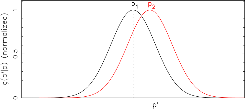
Figure 2: The probability of measuring $p^{\prime}$ when the actual value is $p_{1}$ (black) or $p_{2}$ (red) for the gaussian case.

2.1 Frequentist and Bayesian treatment of measurement errors

Let us for simplicity assume that the probability $g(p^{\prime}|p)$ of measuring parallax $p^{\prime}$ when the actual parallax is $p$ is given by a gaussian

$$g(p^{\prime}|p)dp^{\prime}={1\over\sigma\sqrt{2\pi}}\exp\left({-(p^{\prime}-p)^{2}\over 2\sigma^{2}}\right)dp^{\prime}$$ (1)

where $\sigma$ indicates the measurement error (Fig. 1). For an actual parallax $p$, this implies that in 68% of the cases $|p^{\prime}-p|<\sigma$, i.e. $p^{\prime}-\sigma<p<p^{\prime}+\sigma$. Now consider the measurements for two different actual parallaxes, $p_{1}$ and $p_{2}$. For each we have

$$p^{\prime}-\sigma<p_{1}<p^{\prime}+\sigma\qquad(68\%)$$

$$p^{\prime}-\sigma<p_{2}<p^{\prime}+\sigma\qquad(68\%)$$

The intervals are the same even when $p_{1}$ and $p_{2}$ are different. More generally for any $p_{i}$.

$$p^{\prime}-\sigma<p_{i}<p^{\prime}+\sigma\qquad(68\%)$$

Thus we can state that once a value $p^{\prime}$ has been measured with measurement error $\sigma$ the probability is 68% for any actual value $p_{i}$ that the actual value lies in the interval from $p^{\prime}-\sigma$ to $p^{\prime}+\sigma$. More generally, for each probability we can determine a corresponding interval for $p_{i}$. For example, there is a 90% probability that $1.45(p^{\prime}-\sigma)<p_{i}<1.45(p^{\prime}+\sigma)$. Hence the name frequentist for this approach. However, from the measurement alone we have no information on the probability distribution within this interval.

To obtain that information, we must know how many actual objects there are with $p_{1}$, $p_{2}$,…$p_{i}$, i.e. we must know the distribution $f(p)$ of $p$. After all, a given measrement $p^{\prime}$ may result from any of many actual values $p$, according to Eq. 1. The joint probability $P(p,p^{\prime})$ of actual value $p$ and measured value $p^{\prime}$ is given by

$$P(p,p^{\prime})dpdp^{\prime}=f(p)dp\,g(p^{\prime}|p)dp^{\prime}$$ (2)

and the probability $P(p|p^{\prime})$ of an actual value $p$ in an interval $\Delta p$ for a measured value $p^{\prime}$ is found from this by normalizing over all possibilities:

$$P(p|p^{\prime})\Delta p={f(p)g(p^{\prime}|p)\Delta p\over\int_{p}f(p)g(p^{\prime}|p)dp}$$ (3)

where the denominator acts as a normalisation constant. In this Bayesian approach, $f(p)$ is the prior for $p$.

To apply this to distances we rewrite Eq. 1 in terms of the distance $D=1/p$:

$$g_{D}(p^{\prime}|{1\over D})dp^{\prime}={1\over\sigma\sqrt{2\pi}}\exp\left({-(p^{\prime}-1/D)^{2}\over 2\sigma^{2}}\right)dp^{\prime}$$ (4)

Note that in this equation, $p=1/D$ is fixed, and that the variable is $p^{\prime}$. Hence, in converting Eq. 1 into Eq. 4 no $dp/dD$ term is warranted. For the a priori distance distribution $f_{D}(D)$, with $f_{D}(D)dD=f(p)dp$ (conservation of numbers), we obtain the probability of actual distance $D$ when parallax $p^{\prime}$ is measured as

$$P(D|p^{\prime})\Delta D={f_{D}(D)g_{D}(p^{\prime}|{1\over D})\Delta D\over\int_{p}f_{D}(D)g_{D}(p^{\prime}|{1\over D})dD}$$ (5)

Figure 3: The a priori distribution $f_{D}(D)$ of millisecond pulsars in the direction of PSR J0218+4232 (dotted line, Eqs. 6, 7), and the measured parallax $p^{\prime}=0.16\pm 0.09$ mas, lead to the distance probability distribution given by the solid line, according to Eq. 5. The vertical dashed line indicates the nominal distance $D^{\prime}=1/p^{\prime}$.

2.2 The distance of PSR J0218+4232

Igoshev et al. (2016) illustrate this last equation with the case of the millisecond pulsar PSR J0218+4232 (see Fig. 3). The distance prior is taken from Verbiest et al. (2012), and reflects the fact that we are looking from a location $R_{o}=8.5$ kpc from the galactic center at a distribution around this center in the radial direction, and around the galactic plane in the vertical ($z$) direction. This leads to (in notation slightly altered from that in Verbiest et al. 2012):

$$f_{D}(D)dD=D^{2}R^{1.9}\exp\left(-{D\sin b\over 0.5\,\mathrm{kpc}}-{R\over 1.7\,\mathrm{kpc}}\right)$$ (6)

where $R$ is the distance of the pulsar to the galactic center, projected on the galactic plane:

$$R=\sqrt{{R_{o}}^{2}+(D\cos b)^{2}-2D\cos b\,R_{o}\cos l}$$ (7)

This prior is shown in Figure 3 as a dotted line, for the direction of PSR J0218+4232. Eq. 4 shows that a measured parallax $p^{\prime}$ can result from a range of distances; the probability that a measured $p^{\prime}$ is due to an actual distance $D$ scales with the product of Eq. 4 with the number $f_{D}(D)$ of objects at that distance $D$. After normalization this leads to the probability density function expressed in Eq. 5, and shown for PSR J0218+4232 in Fig. 3.

The factor $g_{D}$ in Eq. 5 leads to a shift of the most probable value of distance $D$ from the peak of $f_{D}(D)$ to values closer to the distance $D^{\prime}=1/p^{\prime}$. Conversely, the factor of the prior $f_{D}(D)$ leads to a shift of the most probable value of $D$ from the nominal distance $D^{\prime}$ towards the peak of the prior distribution.

In the basic form of the Lutz-Kelker effect, for a homogenous distribution $f_{D}(D)\propto D^{2}$, the most probable actual distance is always larger than the nominal distance $D^{\prime}=1/p^{\prime}$. Figure 3 illustrates the fact that the Lutz-Kelker effect in a more general form, i.e. allowing other forms of $f_{D}(D)$, may cause the most probable distance to be lower than the nominal one.

2.3 Confusing frequentist and Bayesian approaches

For a flat prior, $f_{D}(D)=\mathrm{const}$, Eqs. 4 and 5 simplify to

$$P(D|p^{\prime})\Delta D \propto g_{D}(p^{\prime}|{1\over D})\Delta D$$ (8)

$$= {1\over\sigma\sqrt{2\pi}}\exp\left({-(p^{\prime}-1/D)^{2}\over 2\sigma^{2}}\right)\Delta D$$

This equation is very similar to Eq. 4, but there is a crucial difference: the probability of Eq. 4 is normalized by integrating over $p^{\prime}$, the probability of Eq. 8 is normalized by integrating over $D$. Misreading Eq. 8 as valid for an interval $\Delta p^{\prime}$ leads one to write $\Delta p^{\prime}=(1/D^{2})\Delta D$, and thereby add a factor $1/D^{2}$ to Eq. 4. It appears that this is what Faucher-Giguère & Kaspi have done.

In fact, as may be seen from Eq. 5, this corresponds to assuming a prior $f_{D}(D)\propto 1/D^{2}$.

3 Distance from dispersion measure or luminosity

In principle the dispersion measure $DM$, giving the integrated number of electrons between Earth and the pulsar, can be combined with a model for the electron distribution in the Milky Way, to determine the pulsar distance. It is well known that this method gives rather uncertain, and occasionally clearly wrong results (e.g. for B1929+10, see Table 5 in Brisken et al. 2002). Brisken et al., followed by Faucher-Giguère & Kaspi (2006) and by Verbiest (2012), try to circumvent this problem by ‘assigning the $DM$ a gaussian probability distribution function centered on the measured value $DM_{o}$ with a 40% variance’:

$$f_{DM}(DM)\propto\exp\left[-0.5\left({DM-DM_{o}\over 0.4DM_{o}}\right)^{2}\right]$$ (9)

This provides a rough guess of the uncertainty of a distance derived from $DM$ and a model electron dsitribution.

In principle even large measurement uncertainties lead to the correct result, if the measurements are properly weighted. Eq. 9 simplifies the complexity of the galactic electron distribution too much to provide such proper weighting. Note, for example, that the probability for $DM=0$ (hence $D=0$) is non-zero, and indeed the same for all values of $DM_{o}$, no matter how large. Eq. 9 suggests that the error in a distance derived from the dispersion measure is gaussian, where in fact the error is systematic: an error in the electron density model leads to a systematic shift in the derived distance.

Faucher-Giguère & Kaspi (2006), followed by Verbiest et al. (2012), compound the error by adding a multiplication factor $dDM/dD$ in Eq. 9, making an error analogous to the one for distances discussed in Sect. 2.3. This factor has the clearly unphysical effect of concentrating the distance probability in areas of enhanced electron density, since $dDM/dD\propto n_{e}$.

Verbiest et al. (2012) also use the luminosity function to constrain the distance: the luminosity function peaks at low luminosities, hence a pulsar with a given flux is more likely a nearby low-luminosity one than a faraway bright pulsar. In converting a likelihood of luminosity $L$ into a likelihood of distance, Verbiest et al. erroneously introduce a $d\log L/dD$ factor. Igoshev et al. (2016) correct this and show that a wide variety of gamma-ray luminosity functions leads to an isotropic gamma-ray luminosity in excess of 10% of the spindown luminosity for PSR J0218+4232.

Because of the steepness of the luminosity function, straightforward application of the resulting bias pushes the distance probability to the lowest distances allowed by other indicators. Our knowledge of the luminosity function of pulsars depends on our knowledge of distances, and thus in principle the luminosity function and distance distribution of pulsars should be determined together.

4 Velocity from timing and dispersion measure

The annual variation in the difference between heliocentric and geocentric pulse arrival times depends on the celestial position of the pulsar. This dependence may be used to determine the position of the source, and over time its parallax and proper motion, from pulse timing. Hobbs et al. (2005) list a large number of proper motions for pulsars determined with this method. By comparing these proper motions and their uncertainties with the measurements for the same pulsars obtained with VLBI (by Chatterjee et al. 2009, Brisken et al. 2002, Kirsten et al. 2015), we see that the measurement errors given for young (i.e. not recycled) pulsars are of order a hundred times larger for timing measurements than for VLBI. Because of these large uncertainties no timing parallaxes have been determined for young pulsars.

Hobbs et al. (2005) therefore use distances estimated from dispersion measure to convert the proper motions into velocities. Their use of a non-parametric clean algorithm to determine the intrinsic velocity distribution, has the advantage of obviating the need to prescribe a parametrized form of this distribution. However, Hobbs et al. note that the result is well described by a Maxwellian with distribution parameter $\sigma=$ 265 km/s, and argue that the low values of velocity perpendicular to the line of sight observed for some pulsars are the result of projection effects.

One of us, F.V., has always found it hard to accept this, for the following reason. An isotropic Maxwellian may be considered as composed of three gaussians, in three mutually perpendicular directions. If we choose the line of sight as one direction, the two remaining directions are in the celestial plane, and the two gaussians lying in this plane may be combined to give the distribution of $v_{\perp}$. The fraction of velocities in this distribution below any $v_{c}$ may be written (for derivation see Appendix, Eq. 28)

$$f(v_{\perp}<v_{c})=1-e^{{-v_{c}}^{2}/(2\sigma^{2})}$$ (10)

Table 5 of Brisken et al. (2002) lists the nine accurate velocities $v_{\perp}$ known at the time, and of these two have $v_{\perp}<40$ km/s. For $\sigma=265$ km/s and $v_{c}=40$ km/s, the probability for one trial that $v_{\perp}<v_{c}$ follows from Eq. 10 to be about 1%. The probability of finding 2 in 9 trials is 0.4%. This suggests that the fraction of low velocities is underestimated by the analysis of Hobbs et al. (2005). Remarkably, this original argument for the velocity study of Verbunt et al. (2017) study was rather weakened when the accurate proper motion data for 28 pulsars were collected. Not a single new one with $v_{\perp}<40$ km/s was added! The probability of finding 2 in 28 trials is about 4%.

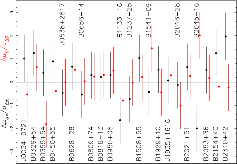
Figure 4: The difference $\Delta\mu_{\alpha*}=\mu_{\alpha*,VLBI}-\mu_{\alpha*,tim}$ between proper motions in the direction of right ascension $\mu_{\alpha*,VLBI}$ and $\mu_{\alpha*,tim}$ measured with VLBI and with timing, respectively, in units of the error in the difference $\sigma_{\Delta\alpha}$ (black); and analogous for the difference $\Delta\mu_{\delta}$ of the proper motions in the direction of declination (red).

As we will see below, a single Maxwellian does underestimate the number of low velocity pulsars, albeit at less low velocities than suggested by the two velocities below 40 km/s. Such an underestimate may arise if Hobbs et al. (2005) underestimate the velocity errors.

Figure 4 compares the proper motions determined from timing with those determined from VLBI, for pulsars with accurate VLBI measurements, by plotting the difference between the proper motions in units of the error in the difference, for the directions of right ascension and of declination separately. The Figure shows that the errors for the timing proper motions, although large, are reliable, in the sense that they are distributed around the correct (VLBI) values as expected. Thus, in velocities determined with proper motions from timing and distances from dispersion measure, the problem for a reliable statistical analysis lies in the distances.

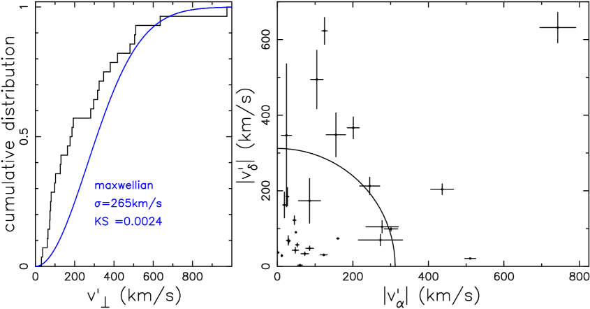
Figure 5: Left: the observed cumulative distribution of $v^{\prime}_{\perp}$ derived from VLBI measurements for 28 pulsars compared with the cumulative distribution of $v_{\perp}$ (Eq. 10) for a Maxwellian with $\sigma=265$ km/s. Right: The nominal velocities $|v^{\prime}_{\alpha}|=|\mu^{\prime}_{\alpha*}|/p^{\prime}$ and $|v^{\prime}_{\delta}|=|\mu_{\delta}|/p^{\prime}$. The circle gives the median velocity $v_{\perp,m}$ (Eq. 11) for $\sigma=265$ km/s.

5 Velocity from VLBI measurements

Given the large errors in the velocities derived with distances from the dispersion measure and proper motions from timing, it appears appropriate to make a first effort at determining the velocity distribution on the basis of the smaller sample with VLBI parallaxes and proper motions. With these much smaller errors, exact understanding of the error distribution is less critical. We collect from the literature 28 young (in the sense of not recycled) pulsars for which these data are available. We indicate the measured values and the nominal values derived from them with a prime: parallax $p^{\prime}$ and proper motions $\mu^{\prime}_{\alpha*},\mu^{\prime}_{\delta}$; and nominal distance $D^{\prime}=1/p^{\prime}$ and velocity perpendicular to the line of sight $v^{\prime}_{\perp}=\sqrt{{\mu^{\prime}_{\alpha*}}^{2}+{\mu^{\prime}_{\delta}}^{2}}/p^{\prime}$.

In Figure 5 we show the cumulative distribution of $v^{\prime}_{\perp}$, together with the cumulative distribution according to Eq. 10 for $\sigma=265$ km/s. The Kolmogorov-Smirnov test gives a probability of 0.0024 that the observed distribution is drawn from this distribution. It shows that the Maxwellian predicts too few pulsars with low velocities, up to several hundred km/s. Some caution is required in the interpretation of this result, because the observed distribution shown in Fig. 5 and used in the Kolmogorov-Smirnov test, ignores measurement errors.

In Figure 5 we also show the absolute values of the nominal velocities $v^{\prime}_{\alpha}=\mu^{\prime}_{\alpha*}/p^{\prime}$ and $v^{\prime}_{\delta}=\mu^{\prime}_{\delta}/p^{\prime}$, together with their nominal errors. The median of $v_{\perp}$ is found by equating the cumulative distribution of Eq. 10 to 0.5:

$$1-e^{{-v_{\perp,m}}^{2}/(2\sigma^{2})}=0.5\Rightarrow v_{\perp,m}=\sigma\sqrt{2\ln 2}$$ (11)

This median is also shown in Figure 5. It is seen that the errors in the lower velocities are small, indicating that our conclusion from the Kolmogorov-Smirnov test on $v^{\prime}_{\perp}$ is reliable. Also, only 7 of 28 pulsars have $v_{\perp}$ higher than the median velocity predicted by a Maxwellian with $\sigma=265$ km/s.

Figure 5 strengthens our earlier suspicion that a single Maxwellian underpredicts the number of low-velocity pulsars. For a definite conclusion, however, we must perform an analysis which takes account of the measurement errors properly.

6 The interplay of distance, proper motion and velocity distribution

As a first prior for the intrinsic velocity distribution we consider a single isotropic Maxwellian. Each pulsar velocity is a draw from this Maxwellian, i.e. a draw from each of three gaussians in mutually perpendicular directions. For each pulsar, we choose the three directions along the line of sight and along the directions of increasing right ascension $\alpha$ and declination $\delta$, and thus for the direction along $\alpha$ we have the prior

$$f(v_{\alpha},\sigma)dv_{\alpha}={1\over\sigma\sqrt{2\pi}}e^{-{v_{\alpha}}^{2}/2\sigma^{2}}dv_{\alpha}$$ (12)

and analogously for $v_{\delta}$ and $v_{r}$. The joint probability of measured values for parallax and proper motions $p^{\prime}$, $\mu^{\prime}_{\alpha*}$ and $\mu^{\prime}_{\delta}$ and actual distance and velocities $D$, $v_{\alpha}$, $v_{\delta}$ and $v_{r}$ follows as

$$P_{\mathrm{maxw}} \equiv P_{\mathrm{maxw}}(p^{\prime},\mu^{\prime}_{\alpha*},\mu^{\prime}_{\delta},D,v_{\alpha},v_{\delta},v_{r})$$ (13)

$$= f_{D}f(v_{\alpha},\sigma)f(v_{\delta},\sigma)f(v_{r},\sigma)g_{D}g_{\alpha}g_{\delta}$$

where $f_{D}$ is given by Eqs. 6, 7 and $g_{D}$ by Eq. 4; $f(v_{\alpha},\sigma)$ by Eq. 12, and $f(v_{\delta},\sigma)$ and $f(v_{r},\sigma)$ analogously; and $g_{\alpha}$ and $g_{\delta}$ by

$$g_{\alpha}={1\over\sigma_{\alpha}\sqrt{2\pi}}\exp\left[-\,{(\mu_{\alpha*,G}(D)+v_{\alpha}/D-\mu^{\prime}_{\alpha*})^{2}\over 2{\sigma_{\alpha}}^{2}}\right]$$ (14)

$$g_{\delta}={1\over\sigma_{\delta}\sqrt{2\pi}}\exp\left[-\,{(\mu_{\delta,G}(D)+v_{\delta}/D-\mu^{\prime}_{\delta})^{2}\over 2{\sigma_{\delta}}^{2}}\right]$$ (15)

where $\sigma_{\alpha}$ and $\sigma_{\delta}$ are the measurement errors in $\mu_{\alpha*}$ and $\mu_{\delta}$, respectively, and $\mu_{\alpha*,G}(D)$ and $\mu_{\delta,G}(D)$ the corrections due to galactic rotation, between the local standards of rest at the position of the Sun and the pulsar. These corrections are necessary, because we are interested in the peculiar velocity of the pulsar, not including the apparent velocity due to galactic rotation. Because most pulsars with an accurate parallax are nearby, these corrections generally are small.

To obtain the value of the scale parameter $\sigma$ which gives the most likely correspondence with the measurements, we must consider the contributions to the likelihood of all distances and velocities, i.e. integrate Eq. 13 over $D$, $v_{\alpha}$, $v_{\delta}$ and $v_{r}$. The integral over $v_{r}$ is 1; the integrals over $v_{\alpha}$ and $v_{\delta}$ are more involved, but can be done analytically. The resulting likelihood is (Verbunt et al. 2017):

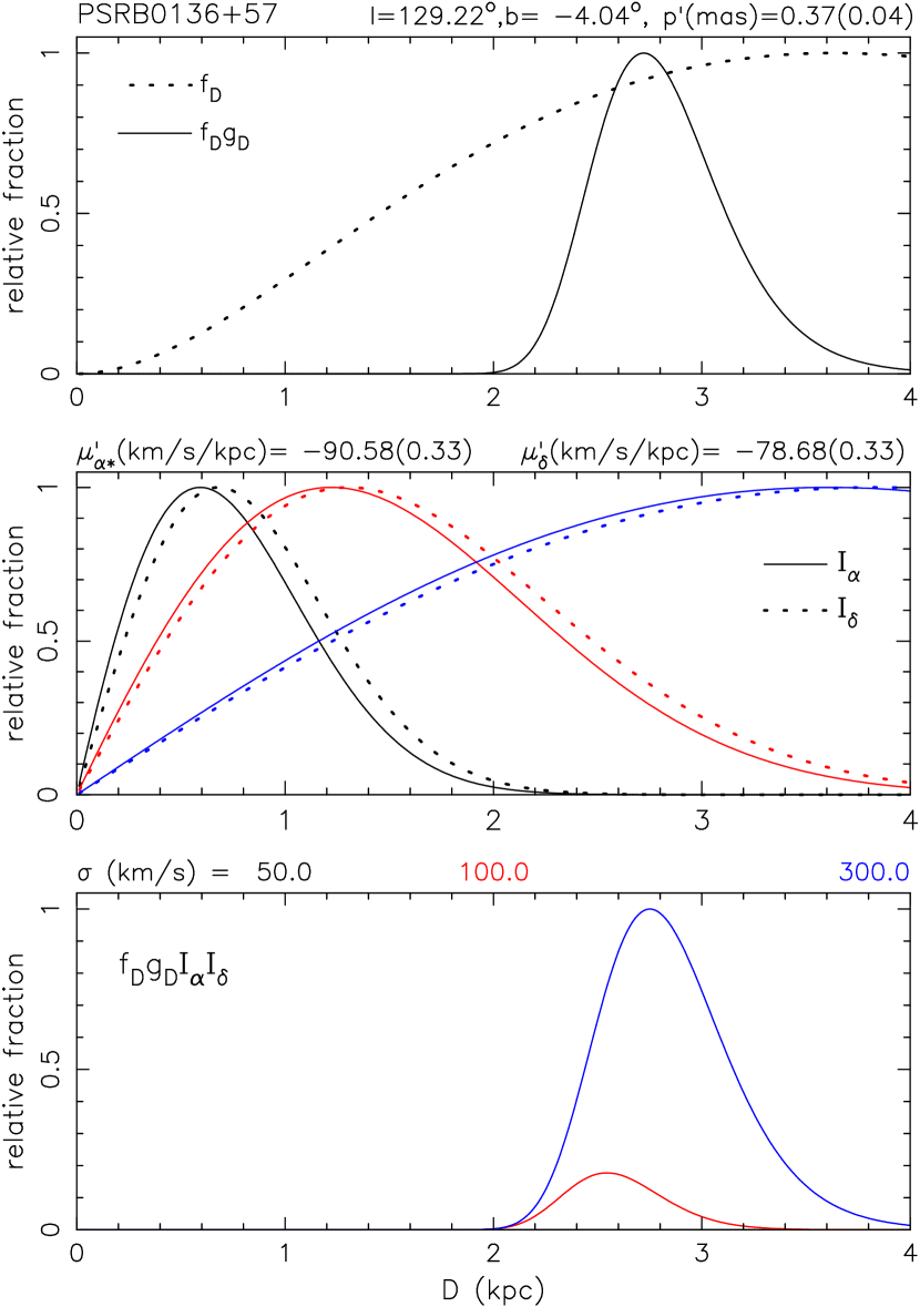
Figure 6: The integrand of Eq. 16. The distance implied by the parallax and galactic pulsar distribution in the direction of PSR B0136+57 (top frame), combined with the proper motion ($\mathcal{I}_{\alpha}$, $\mathcal{I}_{\delta}$, Eq. LABEL:e:ialpha, middle frame) implies a large velocity and favours a Maxwellian with high scale parameter $\sigma$. The curves in the top and middle frame are normalized to maximum value 1. The lower frame shows the integrand of Eq. 16, normalized such that the area under the curve is proportional to the likelihood $L_{\mathrm{maxw}}(\sigma)$ (Eq. 16).

$$L_{\mathrm{maxw}}(\sigma) = \int_{0}^{D_{\mathrm{max}}}\int_{0}^{\infty}\int_{0}^{\infty}\int_{0}^{\infty}P_{\mathrm{maxw}}dDdv_{\alpha}dv_{\delta}dv_{r}$$ (16)

$$= \mathcal{C}\int_{0}^{D_{\mathrm{max}}}\,f_{D}g_{D}\mathcal{I}_{\alpha}\mathcal{I}_{\delta}dD$$

where $\mathcal{C}$ is a constant, ${D_{\mathrm{max}}}$ the maximum distance (we use ${D_{\mathrm{max}}}=10$  kpc; beyond this distance the factor $g_{D}$ according to Eq. 4 ensures that the integrand is effectively zero for the pulsars in our sample), and we define

$$\mathcal{I}_{\alpha} \equiv \left(1+{\sigma^{2}\over D^{2}{\sigma_{\alpha}}^{2}}\right)^{-1/2}\exp\left[-{1\over 2}{(D\,\mu_{\alpha*,G}-D\,\mu^{\prime}_{\alpha*})^{2}\over\sigma^{2}+D^{2}{\sigma_{\alpha}}^{2}}\right]$$

$$\mathcal{I}_{\delta} \equiv \left(1+{\sigma^{2}\over D^{2}{\sigma_{\delta}}^{2}}\right)^{-1/2}\exp\left[-{1\over 2}{(D\,\mu_{\delta,G}-D\,\mu^{\prime}_{\delta})^{2}\over\sigma^{2}+D^{2}{\sigma_{\delta}}^{2}}\right]$$

The effect of the separate contributors to the integrand of Eq. 16 is shown in Figure 6, for the case of PSR B0136+57. The observational data $p^{\prime}$, $\mu^{\prime}_{\alpha*}$ and $\mu^{\prime}_{\delta}$ for this pulsar are taken from Chatterjee et al. (2009). We convert the proper motion with

$$\mu(\mathrm{km/s/kpc})=4.74\mu(\mathrm{mas/yr})$$ (18)

The accurate parallax and proper motion imply a velocity of several hundred km/s: the nominal projected velocity is $v^{\prime}_{\perp}=324$ km/s. When we compare the probability of such a velocity for three different Maxwellians, with $\sigma=50$, 100, and 300 km/s respectively, the probability of the one with $\sigma=300$ km/s is highest.The probability of the Maxwellian with $\sigma=100$ km/s is significantly lower, and the Maxwellian with $\sigma=50$ km/s is virtually excluded (its integrand invisible in Figure 6).

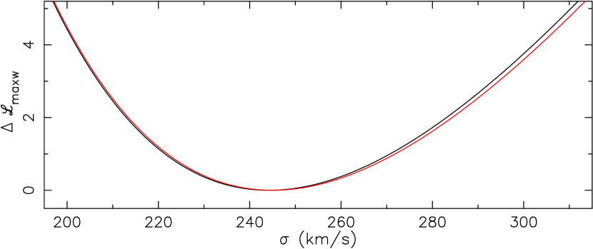
Figure 7: $\mathcal{L}_{\mathrm{maxw}}$ according to Eq. 19 as a function of the Maxwellian scale parameter $\sigma$. The black curve shows the result of the full calculation. The red curve, almost indistinguishable, shows the result when corrections $\mu_{\alpha*,G}$ and $\mu_{\delta,G}$ for galactic rotation are omitted.

6.1 Description with a single Maxwellian

To determine the best value of $\sigma$ for the complete set of 28 pulsars, Verbunt et al. (2017) first compute $L_{\mathrm{maxw}}(\sigma)$ according to Eq. 16 for each of them, integrating numerically over $D$. From these likelihoods the deviance is computed as

$$\mathcal{L}_{\mathrm{maxw}}(\sigma)=-2\sum_{i=1}^{N}\ln L_{\mathrm{maxw},i}(\sigma)$$ (19)

where index $i$ labels the pulsar. With this definition of the deviance, the best value $\sigma_{\mathrm{opt}}$ is the one that minimizes $\mathcal{L}_{\mathrm{maxw}}$ (and thus maximizes the product of the likelihoods), and the differences

$$\Delta\mathcal{L}_{\mathrm{maxw}}\equiv\mathcal{L}_{\mathrm{maxw}}(\sigma)-\mathcal{L}_{\mathrm{maxw}}(\sigma_{\mathrm{opt}})$$ (20)

approximate a $\chi^{2}$ distribution. $\Delta\mathcal{L}_{\mathrm{maxw}}$ is shown as a function of $\sigma$ in Fig. 7. The minimum of $\mathcal{L}_{\mathrm{maxw}}$ occurs at $\sigma_{\mathrm{opt}}\simeq 245$ km/s.

To see the effect of the corrections for galactic rotation to the observed proper motion, we also perform a calculation in which these corrections are omitted, i.e. in which $\mu_{\alpha*,G}$ and $\mu_{\delta,G}$ in Eqs. 16 and LABEL:e:ialpha are put to zero. The result is the same within the uncertainty.

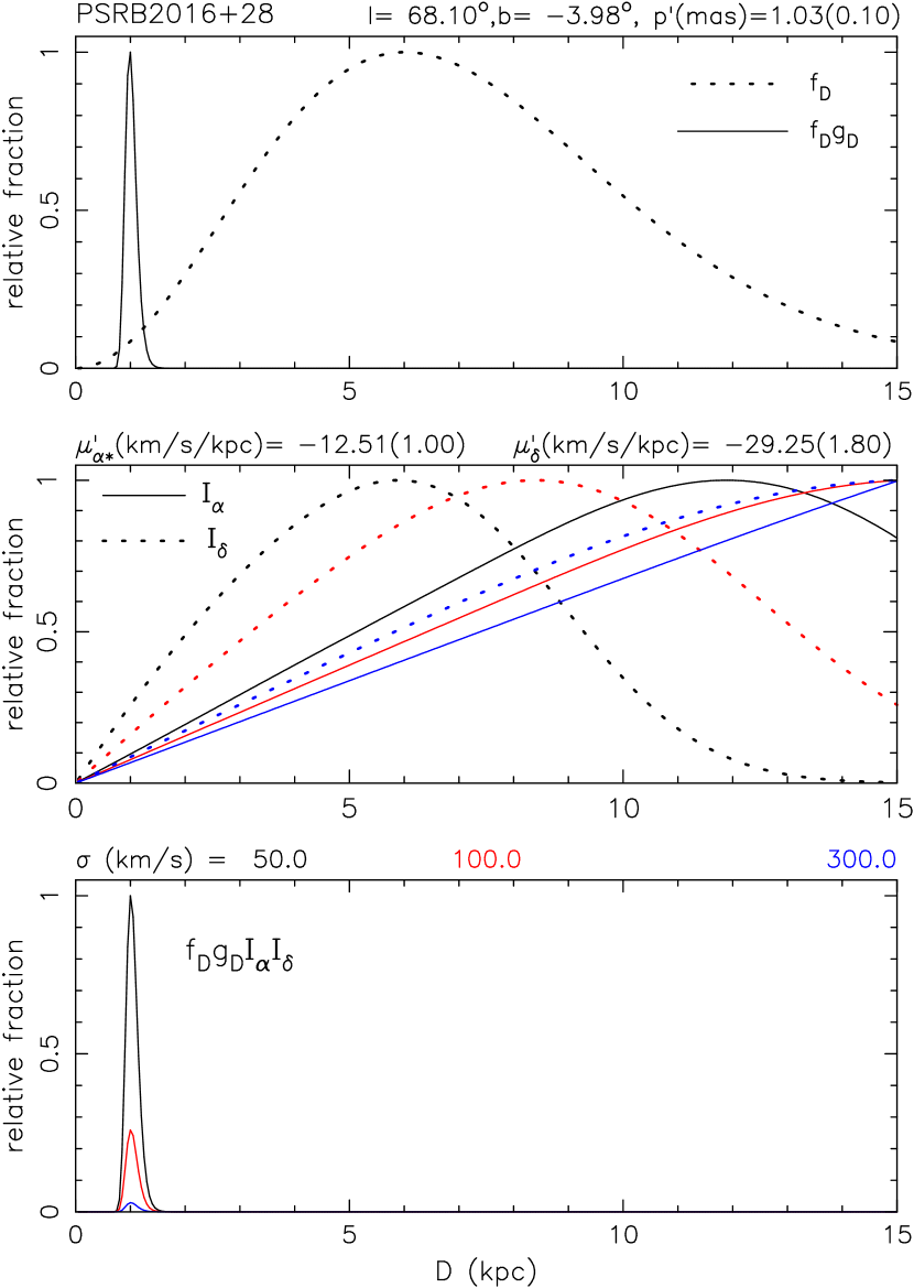
Figure 8: The integrand of Eq. 16, as Figure 6, but now for PSR B2016+28. In this case the parallax and galactic pulsars distribution (top frame) and proper motion (middle frame) imply a small projected velocity $v^{\prime}_{\perp}$. This favours the Maxwellian with low scaling parameter $\sigma=50$ km/s.

6.2 Description with two Maxwellians

As argued in Section 5, a single Maxwellian is not a good description of the observed velocity distribution. To illustrate this,we show in Figure 8 that the data for PSR B2016+28 (taken from Brisken et al.  2002) imply a low projected velocity: $v^{\prime}_{\perp}=31$ km/s. From the three Maxwellians considered, this velocity clearly favours the one with $\sigma=50$ km/s.

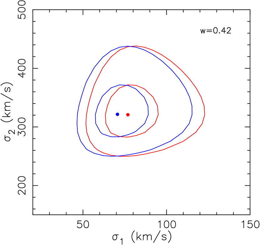
Figure 9: Red: Contours indicating the allowable range of the best solution for two Maxwellians, for $w=0.42$. The best solution is given as a point, the contours contain 68% and 95% probability ($\Delta\mathcal{L}_{2\mathrm{maxw}}=1$ and $\Delta\mathcal{L}_{2\mathrm{maxw}}=4$, respectively). Blue: the same for a model in which the corrections for galactic rotation are omitted.

As a second approach to the determination of the intrinsic velocity distribution of young pulsars, we therefore describe it with the sum of two Maxwellians:

$$f_{v}(\vec{\sigma})=\sqrt{\frac{2}{\pi}}v^{2}\left[\frac{w}{\sigma_{1}^{3}}\exp\left(-\frac{1}{2}\frac{v^{2}}{\sigma_{1}^{2}}\right)+\frac{(1-w)}{\sigma_{2}^{3}}\exp\left(-\frac{1}{2}\frac{v^{2}}{\sigma_{2}^{2}}\right)\right]$$ (21)

with the parameter vector $\vec{\sigma}=w,\sigma_{1},\sigma_{2}$. In analogy we Eqs. 16, 19, 20 we now have

$$L_{2\mathrm{maxw}}(\vec{\sigma})=wL_{\mathrm{maxw}}(\sigma_{1})+(1-w)L_{\mathrm{maxw}}(\sigma_{2})$$ (22)

$$\mathcal{L}_{2\mathrm{maxw}}(\vec{\sigma})=-2\sum_{i=1}^{N}\ln L_{2\mathrm{maxw},i}(\vec{\sigma})$$ (23)

$$\Delta\mathcal{L}_{2\mathrm{maxw}}(\vec{\sigma})\equiv\mathcal{L}_{2\mathrm{maxw}}(\vec{\sigma})-\mathcal{L}_{2\mathrm{maxw}}(\vec{\sigma}_{\mathrm{opt}})$$ (24)

Verbunt et al. (2017) compute $L_{\mathrm{maxw}}(\sigma)$ on a grid of $\sigma$ values with a spacing of 1 km/s, and use the amoeba routine from Press et al. (1986) to determine the values of $\vec{\sigma}_{\mathrm{opt}}$ that minimize $\mathcal{L}_{2\mathrm{maxw}}$. They find that the best description of the velocity distribution is the combination of 42% of the pulsars in a Maxwellian with $\sigma_{1}=77$ km/s with a 58% in a Maxwellian with $\sigma_{2}=320$ km/s. Comparing the best solution for two Maxwell- ians with that for one Maxwellian, Verbunt et al. find $\mathcal{L}_{2\mathrm{maxw}}(\vec{\sigma}_{\mathrm{opt}})-\mathcal{L}_{\mathrm{maxw}}(\sigma_{\mathrm{opt}})=-14$. For two added parameters this difference indicates that the solution with two Maxwellians is significantly better.

The choice of $\mathcal{L}_{\mathrm{2maxw}}$ according to Eq. 22 implies that the distribution of $\Delta\mathcal{L}_{2\mathrm{maxw}}(\vec{\sigma})$ approximates a $\chi^{2}$ distribution. Thus we draw find the 68% and 95% probability contours in the $\sigma_{1}$ - $\sigma_{2}$ plane as delineated by $\Delta\mathcal{L}_{2\mathrm{maxw}}(\vec{\sigma})=1$ and $\Delta\mathcal{L}_{2\mathrm{maxw}}(\vec{\sigma})=4$, respectively. This is shown in Figure 9.

To gauge the effect of the corrections for galactic rotation, we show in the same Figure the results for a computation in which these corrections were set to zero. This leads to a marginal shift to a lower value (71 km/s) for $\sigma_{1}$. The value of $\sigma_{2}$ is not affected.

7 Conclusions

The distance derived from a parallax measurement of a single pulsar is subject to bias, because the distance prior of pulsars is not constant. Application to pulsar PSR J0218+4232 of the correct method for a realistic spatial distribution of millisecond pulsars shows that the isotropic gamma-ray flux of this recycled pulsar is more than 10% of its spindown luminosity.

For the determination of spatial velocities of young, in the sense of not recycled, pulsars we only have measurements of the projections $v_{\perp}$ of these velocities on the celestial sphere. The most direct measurements of $v_{\perp}$ are obtained from VLBI observations of parallax and proper motion. Timing observations can also be used, but the measurement uncertainties are generally several orders of magnitude larger, allowing for determinations of proper motions, but only giving upper limits to the parallaxes. Indirect measurements of distances from disperions measures depend on models for the electron distribution in the Milky Way, and as a result the uncertainties in the distances thus derived are large, and not gaussian but systematic.

Detailed analysis of the parallaxes and proper motions of 28 pulsars confirms the suspicion based on a rough analysis that a single Maxwellian does not describe the velocity distribution of these pulsars. A description with two Maxwellians is significantly better, and finds as a best solution that 42% of the pulsars follow a Maxwellian with distribution parameter $\sigma_{1}=77$ km/s, and 58% a Maxwellian with $\sigma_{2}=320$ km/s. This detailed analysis considers pulsar velocities with respect to their local standard of rest, and to do so applies corrections for galactic rotation. At the current level of accuracy, however, it turns out that these corrections do not have a significant impact on the result.

The number of 28 pulsars for which accurate measurements are availabe is too small to conclude that the velocity distribution is indeed given by the sum of two Maxwellians. It is clear that pulsars have a wide range of velocities, but to determine the exact form of the distribution, accurate measurements of more pulsars are necessary.

Appendix A The Maxwellian velocity distribution and its projection

The Maxwellian velocity distribution may be written

$$f(v)dv=\sqrt{2\over\pi}{v^{2}\over\sigma^{3}}e^{-v^{2}/(2\sigma^{2})}dv$$ (25)

In the isotropic case, the Maxwellian can be decomposed in three gaussian distributions with the same $\sigma$ but otherwise independent, along three mutually perpendicular directions. In the $x$-direction, for example, we have

$$f(v_{x})dv_{x}={1\over\sigma\sqrt{2\pi}}e^{-{v_{x}}^{2}/(2\sigma^{2})}dv_{x}$$ (26)

Choosing the $z$-direction along the line of sight, we find for the velocity perpendicular to the line of sight

$$f(v_{\perp})dv_{\perp} = {1\over 2\pi\sigma^{2}}e^{-(v_{x}^{2}+v_{y}^{2})/(2\sigma^{2})}dv_{x}dv_{y}$$ (27)

$$= {1\over\sigma^{2}}e^{-v_{\perp}^{2}/(2\sigma^{2})}v_{\perp}dv_{\perp}$$

The cumulative distribution of $v_{\perp}$ follows as

$$f(v_{\perp}<v_{c}) = \int_{0}^{v_{c}}{1\over\sigma^{2}}e^{-v_{\perp}^{2}/(2\sigma^{2})}v_{\perp}dv_{\perp}$$ (28)

$$= 1-e^{{-v_{c}}^{2}/(2\sigma^{2})}$$

References

- [1] Bailer-Jones, C.A.L. 2015, PASP, 127, 994.
- [2] Blaauw, A. 1985, in Birth and evolution of massive stars and stellar groups, Eds. W. Boland and H. van Woerden, Reidel, Dordrecht, p.211.
- [3] Brisken, W.F., Benson, J.M., Goss, W.M., Thorsett, S.E. 2002, Astroph. J., 571, 906.
- [4] Brown, A.G.A., Arenou, F., van Leeuwen, F., Lindegren, L., Luri, X. 1997, in ESA Symposium Hipparcos-Venice 1997. ESA SP 402, 63
- [5] Chatterjee, S., Brisken, W.F., Vlemmings, W.H.T., et al. 2009, Astrophys.J., 698, 250.
- [6] Faucher-Giguère, C.-A., Kaspi, V.M. 2006, Astroph. J., 643, 332.
- [7] Feast, M. 2002, MNRAS, 337, 1035.
- [8] Francis, C. 2014, MNRAS, 444, L6.
- [9] Hartman, J.W., Bhattacharya, D., Wijers, R., Verbunt, F. 1997, Astron. Astrophys., 322, 477.
- [10] Hobbs, G., Lorimer, D.R., Lyne, A.G., Kramer, M. 2005, MNRAS, 360, 974.
- [11] Igoshev, A., Verbunt, F., Cator, E. 2016, Astron. Astrophys., 591, A123.
- [12] Kirsten, F., Vlemmings, W., Campbell, R.M., Kramer,M., Chatterjee, S. 2015, Astron. Astrophys., 577, A111.
- [13] Lutz, T.E., Kelker, D.H. 1973, PASP, 85, 573.
- [14] Press, W.H., Flannery, B.P., Teukolsky, S.A., Vetterling, W.T. 1986, Numerical Recipes. The art of scientific computing, Cambridge University Press, Cambridge, p.289.
- [15] Sandage, A., Saha, A. 2002, Astron. J., 123, 2047.
- [16] Verbiest, J.P.W., Lorimer, D.R., McLaughlin, M.A. 2010, MNRAS, 405, 564.
- [17] Verbiest, J.P.W., Weisberg, J.M., Chael, A.A., Lee, K.J., Lorimer, D.R. 2012, Astrophys. J., 755, 39
- [18] Verbiest, J.P.W., Lorimer, D.R. 2014, MNRAS, 444, 1859.
- [19] Verbunt, F., Igoshev, A., Cator, E. 2017, Astron. Astrophys., submitted (arxiv1708.08281)