The build up of the correlation between halo spin and the large scale structure

Abstract

Both simulations and observations have confirmed that the spin of haloes/galaxies is correlated with the large scale structure (LSS) with a mass dependence such that the spin of low-mass haloes/galaxies tend to be parallel with the LSS, while that of massive haloes/galaxies tend to be perpendicular with the LSS. It is still unclear how this mass dependence is built up over time. We use N-body simulations to trace the evolution of the halo spin-LSS correlation and find that at early times the spin of all halo progenitors is parallel with the LSS. As time goes on, mass collapsing around massive halo is more isotropic, especially the recent mass accretion along the slowest collapsing direction is significant and it brings the halo spin to be perpendicular with the LSS. Adopting the $fractional$ $anisotropy$ (FA) parameter to describe the degree of anisotropy of the large-scale environment, we find that the spin-LSS correlation is a strong function of the environment such that a higher FA (more anisotropic environment) leads to an aligned signal, and a lower anisotropy leads to a misaligned signal. In general, our results show that the spin-LSS correlation is a combined consequence of mass flow and halo growth within the cosmic web. Our predicted environmental dependence between spin and large-scale structure can be further tested using galaxy surveys.

1 Introduction

In the currently favoured model for structure formation, initial seeds of perturbation in the early universe were amplified by gravitational instability and dark matter haloes were formed in the regions where the linear density contrast reach some threshold (Gunn & Gott, 1972). On large scales, the matter distribution is characterized by the cosmic web (Bond & Myers, 1996). As dark matter haloes are residing in different cosmic environments (voids, sheets, filaments, clusters) and mass is continuously flowing out of voids, going to sheets, filaments and finally into clusters (Zel’dovich, 1970), it is strongly expected that the halo properties are closely related to their cosmic environment or the nearby large-scale structure (LSS). Numerous studies, especially those using N-body simulations, have confirmed a few correlations between halo properties and the LSS (e.g., Hahn et al., 2007a, b).

Among those various kinds of correlations, the halo spin-LSS is of great interest since it is a result of halo formation in the tidal field exerted by the mass on large scales, and this correlation can be directly predicted by the linear perturbation theory (e.g., Hoyle, 1951; Peebles, 1969; Doroshkevich, 1970; White, 1984; Barnes & Efstathiou, 1987). The tidal torque theory (TTT) predicts that the halo spin has a tendency to align with the intermediate axis of the LSS (e.g., Bond & Myers, 1996; van de Weygaert & Bertschinger, 1996; van Haarlem & van de Weygaert, 1993) under the assumption that the halo inertia tensor is not correlated with the LSS. Although this assumption is not always true Lee & Pen (2000), it is generally found from simulations that the halo spin does have a tendency to align with the intermediate axis of the LSS (Aragón-Calvo et al., 2007; Hahn, Teyssier, & Carollo, 2010; Libeskind et al., 2012; Chen et al., 2016), consistent with the TTT predictions (e.g., Navarro et al., 2004).

Although the predicted correlation between halo spin and the intermediate axis of the LSS is confirmed by N-body simulations, a comparison with the observational data is not trivial. That is because the middle axis of LSS in a filamentary structure is not prominent and thus being difficult to be identified. As the mass along the least compressed direction (later labelled as $\,{\bm{e_{3}}}$) is relatively easy to be identified, most studies have focused on the spin-e3 correlation. Aragón-Calvo et al. (2007) firstly reported that, although this correlation is weak, the signal is highly confident and depends on halo mass. The spin of low-mass haloes have a tendency to align (parallel) with the filament, and that of high-mass haloes are prone to be perpendicular with the filament. This mass dependence and its redshift evolution are later confirmed by many studies which used N-body and hydro-dynamical simulations (Hahn et al., 2007a; Zhang et al., 2009; Codis et al., 2012; Trowland, Lewis, & Bland-Hawthorn, 2013; Libeskind et al., 2013; Forero-Romero, Contreras, & Padilla, 2014; Welker et al., 2014; Dubois et al., 2014; Laigle et al., 2015; Wang & Kang, 2017). Indeed, such a spin-LSS correlation with a galaxy mass (morphology) dependence is also found in the observational data of the SDSS (Tempel & Libeskind, 2013).

The mass dependence of the spin-e3 correlation or the flip of this relation can be understood by studying the halo mass accretion history, as halo spin is a result of mergers and conservation of angular momentum (e.g., Aubert, Pichon, & Colombi, 2004; Bailin & Steinmetz, 2005). It was previously found from simulations that most subhaloes are accreted along filaments (e.g., Wang et al., 2005; Libeskind et al., 2014; Wang et al., 2014; Shi, Wang, & Mo, 2015), but a universal direction of mass accretion is unable to explain the flip of the spin-e3 correlation for low-mass haloes. Kang & Wang (2015) used high-resolution simulations to resolve the formation history of low-mass haloes and they found that mass accretion is indeed not universal, and the accretion of subhaloes in low-mass haloes are perpendicular to the filament. This non-universal mass accretion can well explain the flip of the spin-e3 relation. In addition, the mass accretion pattern can be understood in a wider context of mass flow within the cosmic web. By tracing the mass flow in different cosmic environments, a few studies (Codis et al., 2012; Welker et al., 2014; Laigle et al., 2015) pointed out that low-mass haloes are mainly formed by smoothing accretion through the wind of flows embedded in misaligned walls, and massive haloes are products of major mergers in filaments. Wang & Kang (2017) further find that the spin-e3 correlation is closely related to halo formation time and the transition time when the halo environment changes.

Although those above studies provide a good explanation for the mass dependence of halo spin-e3 correlation, it is not clear how this correlation is built up in detail. For example, for massive haloes with the spin perpendicular to the filament, if we trace them back to higher redshift, should we see a parallel signal between the progenitors’ spin and the filament? How is this spin flip related to the halo mass growth history and the velocity of accreted subhaloes? Other than these questions, we also want to investigate if the spin-e3 correlation depends on the properties of the cosmic web, such as the degree of anisotropy of the LSS. These are the main motivations of this work. Our paper is organized as follows. Sec. 2 presents the simulation data, the method to quantify the halo environment and the halo spin-e3 correlation. In Sec. 3 we show the results in detail including the effects of smoothing length, the evolution of the spin-e3 relation, the dependence of the spin-e3 correlation on the anisotropy of the cosmic web. Conclusions and Discussion are presented in Sec. 4.

2 Simulation and Method

The simulation data used in this work is the same as that used in our two previous papers (Kang & Wang, 2015; Wang & Kang, 2017). In Kang & Wang (2015) we study the accretion of halo mass and its relation with halo major axis and the large-scale environment. In the second paper, we investigate the spin-LSS correlation with dependence on halo formation time and the transition time when the halo environment changes. Readers interested in these studies can refer to those two papers. In the following, we shortly introduce the data and method to classify halo environment.

The N-body simulation was run using the GADGET-2 code (Springel, 2005) and it follows $1024^{3}$ particles in a periodic box of $200\,{\rm Mpc}/h$ with cosmological parameters from the $WMAP7$ data (Komatsu et al., 2011) namely: $\Omega_{\Lambda}=0.73$, $\Omega_{m}=0.27$, $h=0.7$ and $\sigma_{8}=0.81$. The particle mass in this simulation is $5.5\times 10^{8}\,{\rm M}_{\odot}/h$ and 60 snapshots are stored from redshift 10 to 0. We identify dark matter haloes from the simulation using the standard friends-of-friends (FOF) algorithm (Davis et al., 1985) with a linking length that is 0.2 times the mean inter-particle separation. For each FOF halo, we determine its virial radius, defined as the radius centred on the most bound particle inside of which the average density is $200$ times the average density of the universe (Bryan & Norman, 1998). The mass inside the virial radius is called the virial mass $M_{vir}$. We use the SUBFIND algorithm (Springel et al., 2001) to identify subhaloes in each FOF halo, and construct their merger trees (see Kang et al., 2005, for details). Usually, each halo has more than one progenitor at earlier times, and we refer to the most massive one as the main progenitor. By tracing the main progenitor back in time we can obtain the main formation history of the halo. We will use the merger trees to study how the spin-LSS correlation is built up with time in Sec. 3.2.

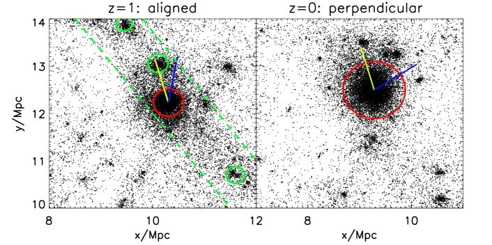
Figure 1: Left: the 2-D mass distribution around a host halo (with mass $\sim 5\times 10^{11}\,{\rm M}_{\odot}/h$) at redshift $z=1$. The red circle denotes its virial radius, and cyan circles denote those subhaloes (haloes) that will merge with the host halo in a short time. The region between the two cyan dashed lines indicates a filamentary structure around the host halo. Right: 2-D slice at redshift $z=0$ around the descendant halo. The halo (with mass $\sim 3\times 10^{13}\,{\rm M}_{\odot}/h$) is the descendant of those shown in the left panel. In this example, the LSS environment of the host halo changes from filament to cluster.

The spin $J$ of a halo is measured as,

$$\bm{J}=\sum_{i=1}^{N}m_{i}\bm{r_{i}}\times(\bm{v_{i}}-\bm{\bar{v}}),$$ (1)

where $m_{i}$ is the particle mass, $\bm{r_{i}}$ is the position vector of particle $\bm{i}$ relative to the halo centre, which is defined as the position of the most bound particle in the halo. $\bm{v_{i}}$ is the velocity of particle $\bm{i}$, and $\bm{\bar{v}}$ is the mean velocity of all halo particles.

To determine the large scale environment of each halo, we employ the method of Hessian matrix used in many previous works (e.g. Aragón-Calvo et al., 2007; Zhang et al., 2009; Kang & Wang, 2015). The Hessian matrix of the smoothed density field at the halo position is defined as:

$$H_{ij}=\frac{\partial^{2}\rho_{s}(\bm{x})}{\partial x_{j}\partial x_{j}},$$ (2)

where $\rho_{s}(\bm{x})$ is the smoothed density field. The eigenvalues of the Hessian matrix are sorted ($\lambda_{1}<\lambda_{2}<\lambda_{3}$), and the eigenvectors are marked as $\,{\bm{e_{1}}}$, $\,{\bm{e_{2}}}$ and $\,{\bm{e_{3}}}$, respectively. According to the Zel’dovich approximation (Zel’dovich, 1970), the eigenvalues of the tidal field can be used to define the large scale environment of each dark matter halo. The number of positive eigenvalues is used to classify the environments of a halo as (Hahn et al., 2007a, b; Zhang et al., 2009),

• $cluster$: no positive eigenvalue;

• $filament$: one positive eigenvalue;

• $sheet$: two positive eigenvalues;

• $void$: three positive eigenvalues;

In N-body simulations, the density field is discontinuous, so it is necessary to smooth the particle distributions. The commonly used way is to divide the simulation box into a number of uniform grid points, then each particle is assigned to several nearby grid points in an appropriate way, mostly using the Cloud-in-Cell interpolation. The density field can be then obtained by smoothing each grid by using a Gaussian filter $G_{R_{s}}$ with a smoothing scale $R_{s}$.

The smoothing scale $R_{s}$ is not specified by the theory directly but depends on the objects one wants to study. For example, if we want to obtain the large scale environment of a dark matter halo with virial radius $\sim$ $100$ $\rm kpc$, the smoothing scale must be slightly larger than the physical size of this dark matter halo, around a few hundreds kpc. However, it can not be too large, otherwise the surrounding environment will be affected by the distribution of mass on a very larger scale, which is not physically linked to the halo in question. In most works (e.g., Aragón-Calvo et al., 2007; Hahn et al., 2007a, b; Zhang et al., 2009; Codis et al., 2012; Trowland, Lewis, & Bland-Hawthorn, 2013) they used a constant smoothing length of $2\rm Mpc$. For more details on how to properly select the smoothing length, see previous works (e.g., Aragón-Calvo et al., 2007; Hahn et al., 2007a; Forero-Romero, Contreras, & Padilla, 2014).

In this work, we use two kinds of smoothing methods. The first one follows that used in Kang & Wang (2015) in which $R_{s}=X\,{\rm Mpc}/(1+z)$ (Method I), where $X$ is $2$ or $5$. This smoothing length is the same for all haloes but is a function of redshift, as it is more physically reasonable and can better describe the evolution of the large scale environment. Libeskind et al. (2012), instead, suggested that a more physical smoothing length should depend on the mass of the halo and is related to the halo virial radius, $R_{s}=XR_{vir}$ (Method II), where $X$ is between $4$ and $8$. We will later show that our results are not strongly affected by the selection of the smoothing lengths.

In some previous works on the correlation between halo spin and the LSS (e.g., Aragón-Calvo et al., 2007), the direction of the LSS is chosen based on the geometric feature of the structure. For example, in a filament region the LSS is defined as the direction along the filamentary structure, corresponding to $\,{\bm{e_{3}}}$, and in a sheet environment, the direction is chosen to be perpendicular to the sheet plane (the $\,{\bm{e_{2}}}-\,{\bm{e_{3}}}$ plane), so along the $\,{\bm{e_{1}}}$ direction. As pointed out by Libeskind et al. (2014) and Kang & Wang (2015), $\,{\bm{e_{3}}}$ is a good and universal definition of the direction of LSS. For instance, in a filament region, $\,{\bm{e_{3}}}$ along the filamentary structure, and in a cluster region, $\,{\bm{e_{3}}}$ is the latest collapsed, least compressed direction. It is worth noting that when we talk about any correlations with the large-scale environment, it is important to have a consistent definition of the environment. In this work, we thus use the $\,{\bm{e_{3}}}$ as the universal definition of the LSS and use it to specify the correlation between halo spin and the LSS.

The correlation between halo spin and the $\,{\bm{e_{3}}}$ is quantified using their alignment angle, $\cos\theta_{3}$, as,

$$\cos\theta_{3}=\bm{j}\cdot\,{\bm{e_{3}}},$$ (3)

where $\bm{j}$ is the spin vector and $\,{\bm{e_{3}}}$ is the eigenvector calculated by Equation 2 at the position of the halo. If the halo spin is randomly oriented in 3-D space relative to $\,{\bm{e_{3}}}$, the expected value of $<\cos(\theta_{3})>$ is 0.5. In case $<\cos(\theta_{3})>$ is larger than 0.5, we refer it to an alignment (parallel) between the spin and the LSS, and for $<\cos(\theta_{3})>$ lower than 0.5, we call it a mis-alignment (perpendicular) between the spin and the LSS.

3 Results

In this section, we first show the spin-$\,{\bm{e_{3}}}$ correlation with its dependence on smoothing lengths, halo mass and redshift. Then, we trace the haloes back in time to see how the spin-$\,{\bm{e_{3}}}$ correlation is built up for haloes with different masses, and investigate how the flip of the relation is related to their anisotropic mass growth. We will also show that the anisotropy of the halo environment can be quantified using a simple parameter, and it also partly determines the degree of the halo spin-LSS alignment.

3.1 Spin flips

In order to have an intuition about the correlation between halo spin with the LSS and its evolution, in Fig. 1 we show the 2-D mass distribution around a dark matter halo whose virial mass is $\sim 3\times 10^{13}\,{\rm M}_{\odot}/h$ at redshift $z=0$, and its main progenitor is $\sim 5\times 10^{11}\,{\rm M}_{\odot}/h$ at redshift $z=1$. The left panel shows the progenitors at $z=1$, where the main progenitor is marked with a red circle and the other progenitors (for clarity, only three of them are shown) are marked as green circles. The yellow line gives the direction of the LSS ($\,{\bm{e_{3}}}$), which resembles a filamentary structure, and the blue line indicates the spin of the main progenitor. In this case the halo spin is aligned with the LSS. The right panel shows that after mergers the final halo spin is misaligned (or perpendicular) with the direction of the LSS, for which the environment is turned into a cluster region. This particular case shows that in a filamentary structure, the mass is mainly accreted along the filament, and after most of the mass along the filament has collapsed (merged into the main halo), and the LSS environment will possibly evolve into a cluster region, in which the spin is perpendicular to the recently collapsed direction.

Previous studies (Aragón-Calvo et al., 2007; Hahn et al., 2007a) usually investigated the spin-LSS correlations for haloes in sheet and filament environments separately. These studies found that the spin of haloes in sheet tends to lie in the sheet plane, and in filaments there is a transition halo mass around $10^{12}M_{\odot}$, below which halo spin is parallel to filaments and above which the halo spin is perpendicular to the filament. Wang & Kang (2017) find that, similar to the case for the filament, the spin-e3 correlation of haloes in cluster environment also has a mass dependence, and the transition mass is slightly smaller than that in filament. In this work we investigate the spin-LSS correlation for haloes as a whole, and we do not consider halo environment, but just focus on the mass dependence.

In Fig. 2 we show the spin-e3 correlation at $z=0$ with two different smoothing methods. In agreement with a previously similar study by Forero-Romero, Contreras, & Padilla (2014), we find that, without considering halo environment, the spin-e3 correlation is similar to that of haloes in filaments, with a transition mass at which the spin-e3 correlation flips. Note that although the alignment/mis-alignment signal is very weak, it departs significantly from a random distribution, which can be seen from the errorbars on the horizontal dash line. Fig. 2 also shows that adopting different smoothing methods will produce a slightly different transition mass, ranging within a factor of 2 between $7\times 10^{11}M_{\odot}\sim 2\times 10^{12}M_{\odot}$. This transition mass with a weak dependence on smoothing scales is in broad agreement with previous results (Aragón-Calvo et al., 2007; Aragon-Calvo & Yang, 2014; Codis et al., 2012; Pichon et al., 2016; Wang & Kang, 2017). As the effects of the smoothing length are very weak, in the following we will only show results from the second smoothing methods with $R_{s}=4R_{vir}$. We have tested that our results and conclusions are not affected by using other smoothing lengths.

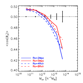
Figure 2: The halo spin-$\,{\bm{e_{3}}}$ correlation at $z=0$ as a function of halo virial mass. The solid (Method I) and dashed (Method II) lines are for two different smoothing methods. The horizontal dashed line corresponds to a random distribution between halo spin and $\,{\bm{e_{3}}}$ of the large scale structure. It is seen that the alignment depends on halo mass, and the flip of this correlation is at around $10^{12}M_{\odot}$ with a slight dependence on the smoothing length. The error bars are calculated by $1/\sqrt{N}$, in which N is the number in each bin. The same method is adopted in following figures.

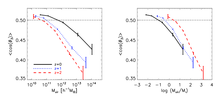
Figure 3: Left: the halo spin-e3 alignment at different redshifts. Right: as the left panel, but the halo mass is normalized by $M_{\star}$, the characteristic mass of halo collapsing at a given redshift. The two panels show different redshift dependence, while the right panel reveals a real evolution pattern at given normalized halo mass (see text for more detail).

In Fig. 3 we show the mass and redshift dependence of the spin-e3 correlations. Note that in the right panel the halo mass is normalized by the characteristic mass of halo collapsing at a given redshift. The left panel shows that the mass dependence of spin-e3 correlation is seen at all redshifts, but the transition mass where the correlation flip from perpendicular to parallel is lower at high redshifts. At given halo mass, the alignment signal is lower at high redshift, indicating that the halo spin is more likely to be perpendicular to the LSS at high redshift. However, this is not an evolution pattern for the spin-e3 relation. As the halo mass also grows with redshift, so we should not inspect the relation of the relation at a given halo mass. More physically interesting results are seen in the right panel of Fig. 3, where the halo mass is normalized by the characteristic mass, $M_{\star}$, which is the typical mass of halo collapsing at a given redshift. The mass $M_{\star}$ can be calculated using the matter power spectrum with a given set of cosmological parameters and a given redshift (see Trowland, Lewis, & Bland-Hawthorn, 2013, for more details). It is seen that for haloes with a given $M_{vir}/M_{\star}$, i.e., the same stages of collapse (Trowland, Lewis, & Bland-Hawthorn (2013)), the alignment signal is higher at high redshift, showing that during the evolution halo spin is more likely to be parallel to the LSS at early times. As time passes by, the alignment becomes weaker and the spin is inclined to be perpendicular to the LSS at low redshift. These redshift dependencies are in broad agreement with previous studies (Hahn et al., 2007a; Trowland, Lewis, & Bland-Hawthorn, 2013).

3.2 Spin evolution and mass accretion anisotropy

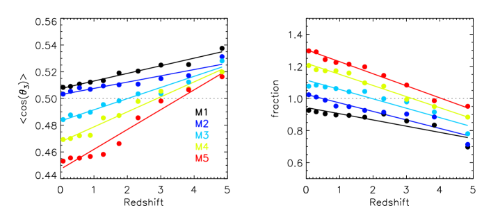
Figure 4: Left: the evolution of the mean cosine of the angle, $<\theta_{3}>$, between the spin of halo’s progenitors and the $\,{\bm{e_{3}}}$ at corresponding redshift. The descendant haloes at $z=0$ are divided into 5 mass bins, marked from $\rm M1$ to $\rm M5$ with increasing mass (see Table. 1). Right: the evolution of the anisotropic mass accretion for haloes in different mass bins. Here $fraction$ is the ratio between the cumulative mass accreted along $\,{\bm{e_{3}}}$ ($0^{\circ}<\theta<45^{\circ}$) and the cumulative accreted mass perpendicular to $\,{\bm{e_{3}}}$ ($45^{\circ}<\theta<90^{\circ}$) at a given redshift bin. The points are the measurements from simulations and the lines are the linear fits to the data, with parameters listed in Table. 2

Table 1: We divide haloes at $z=0$ into five mass bins, from $\rm M1$ to $\rm M5$ with increasing mass. The table lists the range of mass and number of haloes in each mass bin.

sample	Mass range ($z=0$)	Num. of haloes
M1	$[10^{10}-10^{11}]\,{\rm M}_{\odot}/h$	570123
M2	$[10^{11}-10^{12}]\,{\rm M}_{\odot}/h$	174818
M3	$[10^{12}-10^{12.5}]\,{\rm M}_{\odot}/h$	17351
M4	$[10^{12.5}-10^{13}]\,{\rm M}_{\odot}/h$	6207
M5	$>10^{13}\,{\rm M}_{\odot}/h$	2830

Table 2: The parameters obtained from a linear fitting, $y=a*redshift+b$, are listed below. Slopes, zero-points and their errors are signed with $a$, $b$ and $\sigma$, with subscript $\theta$ for the left panel in Fig. 4 and subscript $f$ for the right panel.

sample	$a_{\theta}$	$b_{\theta}$	$\sigma_{a_{\theta}}$	$\sigma_{b_{\theta}}$	$a_{f}$	$b_{f}$	$\sigma_{a_{f}}$	$\sigma_{b_{f}}$
M1	0.0057008	0.507353	0.151267	0.343309	-0.0387258	0.94338	0.187814	0.559281
M2	0.0046992	0.502829	0.150392	0.349159	-0.0530214	1.02523	0.193150	0.540680
M3	0.0083454	0.483183	0.148909	0.354379	-0.0585716	1.11478	0.200449	0.515152
M4	0.0112145	0.467537	0.147422	0.360299	-0.0693331	1.21954	0.210341	0.495142
M5	0.0148303	0.447117	0.146150	0.361961	-0.0751330	1.30434	0.217498	0.476506

In order to understand in detail how the spin-e3 correlation is built up and how it is related to halo mass growth, we trace haloes back in time to study the spin-e3 correlation of their main progenitors with the large scale structure at different redshifts. We select haloes within different mass bins at $z=0$, and in Tab. 1 we list the mass ranges and number of haloes in each mass bins. For each dark matter halo we trace its main progenitor back to higher redshifts, and we also obtain the $\,{\bm{e_{3}}}$ direction of the LSS around each main progenitor using the Hessian matrix method.

In the left panel of Fig. 4, we show the evolution of $\cos\theta_{3}$ between the spin and $\,{\bm{e_{3}}}$ for the main progenitors of haloes selected in five different mass bins at $z=0$, where the halo mass is increasing from the top to the bottom lines. In the right panel, we show the evolution of the anisotropic mass accretion history of those haloes. Here the anisotropic mass accretion parameter $fraction$ is defined as the ratio between the total mass accreted at each redshift by the main progenitor along the $\,{\bm{e_{3}}}$ direction (within an angle between $0^{\circ}$ and $45^{\circ}$), and those accreted perpendicular to $\,{\bm{e_{3}}}$, within an angle between $45^{\circ}$ and $90^{\circ}$. In both panels the lines are the best linear fits to the points with fitted parameters given in Table. 2.

The left panel shows that there is a strong evolution of the alignment between halo spin and $\,{\bm{e_{3}}}$. For massive haloes (red points), their spin is perpendicular to the LSS at lower redshift, but for their main progenitors at high redshifts, such as at $z>3$, the halo spin is parallel to $\,{\bm{e_{3}}}$. For low-mass haloes (black points), their spin is parallel to $\,{\bm{e_{3}}}$ all the time, but the alignment is much better at higher redshift. Of course here the signal is for the average, and it is definitely true that for a single halo its spin evolution can be much more complicated. This plot shows that, on average, at high redshifts the halo spin is more likely to be parallel to the LSS, but with the halo mass growth, the halo spin will more likely evolve into being perpendicular to the LSS, and this evolution is faster for massive haloes. As pointed out in Wang & Kang (2017), this rapid evolution for massive haloes is related to their migration time that massive haloes enter filament earlier, so the mass flow along the filament will lead to a quick spin flip.

The evolution of the halo spin-$\,{\bm{e_{3}}}$ correlation is strongly related to the anisotropic mass accretion history, which is shown in the right panel of Fig. 4. It shows that, at the early time, the mass accretion in all progenitors is mainly perpendicular to the $\,{\bm{e_{3}}}$, and their evolution is dependent on halo mass. For low-mass haloes, the parameter $fraction$ is lower than 1 across the time, but for massive haloes, the mass accretion proceeds to be along the $\,{\bm{e_{3}}}$ at lower redshifts. Under the natural assumption that the orbital angular momentum of accreted mass will be converted to halo spin (Welker et al., 2014), it is easy to understand that once the mass accretion along $\,{\bm{e_{3}}}$ is dominated, the final halo spin will be perpendicular to $\,{\bm{e_{3}}}$, in good agreement with previous work (Libeskind et al., 2014; Kang & Wang, 2015). The transition redshifts for the flip of the spin-$\,{\bm{e_{3}}}$ correlation in the left panel correspond well with those in the right panel for different halo mass bins, showing that the halo spin is strongly correlated with the mass accretion history.

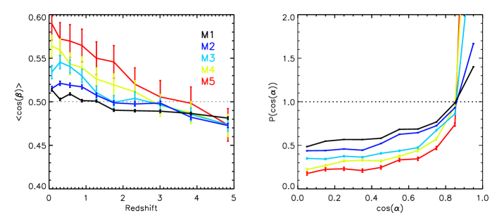
Figure 5: Left panel: the mean $\cos\beta$ as a function of redshift, in which $\beta$ is the angle between the halo velocity vector and the direction of LSS, $\,{\bm{e_{3}}}$. Right panel: the distribution of the angle between the $\,{\bm{e_{3}}}$ at $z=z_{i}$ and the $\,{\bm{e_{3}}}$ at $z=0$. It shows that the $\,{\bm{e_{3}}}$ is better aligned during the halo evolution, especially for massive halos.

On larger scales, the motion of dark matter haloes should follow the mass flow within the cosmic web. Icke & van de Weygaert (1991) suggested that mass and velocity flows are transported in such a way: matter flows out from the void into the sheet plane and then flows inside the sheet plane to the intersection of sheets where the filament is formed. Inside the filament, the mass is mainly flowing along the filamentary structure, and finally into a cluster region where the filaments intersect with each other. Such a model of mass transport within cosmic web is clearly illustrated using simulations. (Cautun et al. (2014), their Fig.35). In the left panel of Fig. 5 we show the evolution of the average angle $<\cos\beta>$ between the halo velocity and the LSS $\,{\bm{e_{3}}}$. The plot shows that, at high redshift, the halo velocity is slightly perpendicular to $\,{\bm{e_{3}}}$, but becomes more parallel to $\,{\bm{e_{3}}}$ at lower redshift. At early times most haloes are in the sheet environment, where the mass flow is mainly from voids and thus being perpendicular to the sheet plane. As time goes on, halo environment is progressively changing into filament or cluster, so the halo velocity is mainly along $\,{\bm{e_{3}}}$. Both the mass and velocity flows well explain the evolution of spin-$\,{\bm{e_{3}}}$ relation as seen in Fig. 4.

Although the halo environment is evolving with time, our definition of $\,{\bm{e_{3}}}$ is the slowest collapsed direction, thus its direction is not expected to change much during the halo evolution. To check this assumption, in the right panel of Fig. 5 we show the distribution of the angle,$\alpha$, between the LSS $\,{\bm{e_{3}}}$ around the main progenitor at $z>0$ with the $\,{\bm{e_{3}}}$ of the descendant halo at $z=0$. Similar with previous results, the $z=0$ descendant haloes are selected in different mass bins. The panel shows that the distribution is skewed to higher $\cos(\alpha)$, indicating that indeed the $\,{\bm{e_{3}}}$ direction does not change much during the evolution. It is also seen that for massive haloes the $\,{\bm{e_{3}}}$ retains its stability much better.

3.3 FA dependence

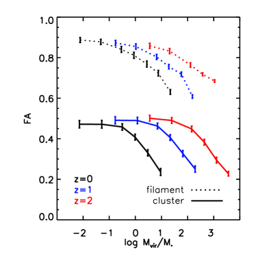
Figure 6: The fractional anisotropic ($\rm FA$) as a function of halo mass for haloes in different environments and redshifts. $\rm FA$ denotes the degree of anisotropy of the large-scale tidal field, where a lower value means that the mass along all the three directions of the tidal field has collapsed, as the case for the cluster. A higher $\rm FA$ means that the mass collapse is highly anisotropic, as the case for a sheet or filament environment.

The above results show that the halo spin-$\,{\bm{e_{3}}}$ correlation depends on the anisotropic mass accretion on large scales. Usually, for haloes in a given cosmic environment, the anisotropic collapse along the eigenvectors of the tidal field might be different. It would be interesting to see if the spin-$\,{\bm{e_{3}}}$ correlation is also dependent on the degree of the anisotropic tidal field. Libeskind et al. (2013) defined an useful parameter, $fractional$ $anisotropy$ (FA), to quantify the degree of anisotropy of the tidal field:

$${\rm FA}=\frac{1}{\sqrt{3}}\sqrt{\frac{(\lambda_{1}-\lambda_{3})^{2}+(\lambda_{2}-\lambda_{3})^{2}+(\lambda_{1}-\lambda_{2})^{2}}{\lambda_{1}^{2}+\lambda_{2}^{2}+\lambda_{3}^{2}}},$$ (4)

where $\lambda_{1},\lambda_{2},\lambda_{3}$ are the eigenvalues of the Hessian matrix of the density field. According to its definition, $\rm FA$ ranges between 0 and 1. In general, a lower FA means an equal collapse along the three eigenvectors, which corresponds to a cluster environment. A higher $\rm FA$ means that the collapse is highly anisotropic and being significant along one direction, usually corresponding to a sheet region.

To understand the effect of FA on the spin-$\,{\bm{e_{3}}}$ correlation, in Fig. 6 we first show the mass dependence of the $\rm FA$ parameters for haloes in different environments and redshifts. The dotted lines are for haloes in filaments and solid lines for haloes in clusters, while the colours denote different redshifts. It is found that at a given redshift and environment, high mass haloes have lower $\rm FA$, and low-mass end haloes have higher $\rm FA$ but with a weak mass dependence. As pointed out by Libeskind et al. (2013), this is a consequence of mass collapse around dark matter haloes, as a halo is more likely to grow when the mass on all directions of the LSS is strongly compressed. The figure also shows that $\rm FA$ is a strong function of environment and redshift. For haloes in clusters, the collapse along all the three eigenvector directions have happened, so the anisotropy is lower. In filament regions, instead, the collapse is mainly on the $\,{\bm{e_{1}}}$ and $\,{\bm{e_{2}}}$ directions, so the anisotropy is systematically higher. We can see that the FA is also lower at low redshift. This is expected as mass collapse progressively proceeds to all directions with increasing time, as predicted by the Zel’dovich theory (Zel’dovich, 1970).

Figure 7: The mean $\rm cos(\theta_{3})$ of cluster haloes (filled circles) and filament haloes (filled upward triangles) as a function of $\rm FA$. Here we only show results at $z=0$ for halos in two mass bins.

In Fig. 7 we show the average alignment signal of spin-$\,{\bm{e_{3}}}$ at $z=0$ as a function of $\rm FA$, for haloes in two mass bins and two environments, respectively. The general trend is that the halo spin tends to be perpendicular to $\,{\bm{e_{3}}}$ with decreasing $\rm FA$. As discussed before, this is expected as a lower $\rm FA$ indicates that the mass along the slowest collapse direction $\,{\bm{e_{3}}}$ also begins, so the mass is basically accreted along $\,{\bm{e_{3}}}$ and results in a perpendicular signal. For the same reason, haloes in cluster regions tend to have a lower alignment between their spin and the LSS. However, it is interesting to see that for haloes with given $\rm FA$ and given environment, there is still a mass dependence such that high-mass haloes have a stronger mis-alignment between their spin and $\,{\bm{e_{3}}}$. This can be explained by the halo formation and the migration time when the halo environment changes. Wang & Kang (2017) have shown that in filament environments, massive haloes form after they enter into filaments, but low-mass haloes form before they enter a filament. The later significant mass accretion in massive haloes along with filament will lead to a stronger mis-alignment between the halo spin and the filament direction $\,{\bm{e_{3}}}$. The results in Fig. 7 show that there is no one single parameter which can fully determine the degree of alignment between the halo spin and the LSS, and the alignment is dependent on halo mass, environment and the anisotropy of the tidal field.

4 Conclusions and discussion

In this paper, we study the correlation between halo spin and the slowest collapse direction, $\,{\bm{e_{3}}}$, of the large scale structure. We investigate how the spin-$\,{\bm{e_{3}}}$ correlation is built up over time, its relation to the anisotropic mass accretion history and the degree of anisotropic collapse on large scales. The main results are summarized as below,

• Similar to previous studies on the halo spin-$\,{\bm{e_{3}}}$ correlation in filament and cluster environments separately, we find that, regardless of the environment, the halo spin-$\,{\bm{e_{3}}}$ relation also has a mass dependence. For low-mass haloes, their spin tends to be parallel to $\,{\bm{e_{3}}}$, and high mass haloes have spin perpendicular with $\,{\bm{e_{3}}}$. The transition mass for the flip of the correlation is around $10^{12}M_{\odot}$, with a slight dependence on the smoothing length. We also find that at a given halo mass, normalized by the characteristic mass of halo collapsing at a given redshift, halo spin is more likely to be parallel to $\,{\bm{e_{3}}}$ at high redshift, but perpendicular to $\,{\bm{e_{3}}}$ at lower redshift.

• By tracing the main progenitor of halo back in time, we study the build up of the halo spin-$\,{\bm{e_{3}}}$ relation at different redshifts. we find that at early times the spin of progenitor haloes tend to be parallel to $\,{\bm{e_{3}}}$, but the final correlation at $z=0$ depends on the mass growth. For massive halo, the mass collapse on large scale is significant and most of the mass accretion is along with the $\,{\bm{e_{3}}}$ direction at low redshift. Under the assumption that the orbital angular momentum is transferred into the halo spin, it is naturally expected that mass accretion along $\,{\bm{e_{3}}}$ will lead to a spin perpendicular to $\,{\bm{e_{3}}}$. Massive haloes have quick evolution with redshift than low-mass ones as they migrate into their current environment earlier, as explained in Wang & Kang (2017).

• The degree of anisotropic collapse along different directions of the tidal field can be described by the parameter $fractional$ $anisotropy$ (FA) proposed by Libeskind et al. (2013). A higher FA means that the collapse on large scale is highly anisotropic, as in the sheet environment, and a lower FA indicates that near equal collapse has happened along all the three directions on large scale, which usually corresponds to a cluster environment. We find that at given halo mass and environment, the spin of halo with lower FA is more mis-aligned with the $\,{\bm{e_{3}}}$. This is because in low FA region matter collapse has happened along the $\,{\bm{e_{3}}}$ direction, leading to a halo spin inclined to be perpendicular to $\,{\bm{e_{3}}}$. However, our results also show that FA is not the only parameter which can fully specify the spin-$\,{\bm{e_{3}}}$ relation, but with additional dependence on halo mass and environment.

Most previous works studied the spin-LSS correlations for haloes in different environments separately. Our study use haloes in different environments as a whole and the definition of LSS is consistent across different environments, thus the conclusion on the spin-LSS relation in this paper is more general. We trace the evolution of the spin-LSS correlation and find that the spin of massive haloes is not born to be mis-aligned (or perpendicular) with the LSS, but it is a consequence of the evolution of halo mass and environment. We also find that the correlation is dependent on the degree of anisotropy of the mass distribution on large scales.

Our results are consistent with the mass flow within the cosmic web as illustrated in Icke & van de Weygaert (1991) and Cautun et al. (2014). At early times, most haloes are formed in highly anisotropic environments, such as sheets, the mass is flowing from voids into the sheet planes along the fast collapsing direction, so the resulted halo spin is parallel to the slowest collapsing direction which lies in the sheet plane. As time goes by, haloes flow into filaments and clusters. Usually massive haloes are migrated into these environments earlier, so most of their mass growth is occurring in filaments or clusters in which the mass flow is mainly along the slowest collapsing direction, then the orbital angular momentum of the accreted mass will be transferred into halo spin, which will then be more likely to be perpendicular with the slowest collapsing direction of the LSS. Such a formation time and transition time dependence are also presented in our previous work by Wang & Kang (2017).

However, due to the complicated interplay between halo mass growth, environment changing and the anisotropy of the large-scale tidal field, we do not find a universal spin-$\,{\bm{e_{3}}}$ correlation, but being a function of redshift and the anisotropy of the LSS. For the first time, we find that the spin-$\,{\bm{e_{3}}}$ correlation is a strong function of the anisotropy of the large-scale environment using N-body simulations. Such an environmental dependence of spin-filament correlation has been reported in observations by Jones, van de Weygaert, & Aragón-Calvo (2010) in which they found that the spin of spiral galaxies is more perpendicular to the spine of the parent filament in the less dense environment. This is qualitatively in agreement with our findings in the paper. It is deserved to investigate the dependence of spin-filament alignment on the anisotropy of the large-scale environment using galaxy surveys in more detail and such a study will shed more light on our understanding of galaxy formation in the cosmic web.

5 Acknowledgments

We thank the referee, Miguel Aragón-Calvo, for careful reading and constructive suggestions which improve the presentation of our paper. We also thank Liang Wang, Simon H. Wang and Emanuele Contini for careful reading and editing of the manuscript. We thank Noam Libeskind, John Peacock, Yanchuan Cai, Cautun Marius, Shi Shao and Mark Neyrinck for discussions. The work is supported by the 973 program (No. 2015CB857003, No. 2013CB834900), the NSFC (No. 11333008), NSF of Jiangsu Province (No. BK20140050). The simulations are run on the supercomputing center of PMO and CAS.

References

- Aragón-Calvo et al. (2007) Aragón-Calvo M. A., Jones B. J. T., van de Weygaert R., van der Hulst J. M., 2007, A&A, 474, 315
- Aragón-Calvo et al. (2007) Aragón-Calvo M. A., van de Weygaert R., Jones B. J. T., van der Hulst J. M., 2007, ApJ, 655, L5
- Aragon-Calvo & Yang (2014) Aragon-Calvo M. A., Yang L. F., 2014, MNRAS, 440, L46
- Aubert, Pichon, & Colombi (2004) Aubert D., Pichon C., Colombi S., 2004, MNRAS, 352, 376
- Bailin & Steinmetz (2005) Bailin J., Steinmetz M., 2005, ApJ, 627, 647
- Barnes & Efstathiou (1987) Barnes J., Efstathiou G., 1987, ApJ, 319, 575
- Bond & Myers (1996) Bond J. R., Myers S. T., 1996, ApJS, 103, 1
- Bryan & Norman (1998) Bryan G. L., Norman M. L., 1998, ApJ, 495, 80
- Cautun et al. (2014) Cautun M., van de Weygaert R., Jones B. J. T., Frenk C. S., 2014, MNRAS, 441, 2923
- Chen et al. (2016) Chen S., Wang H., Mo H. J., Shi J., 2016, ApJ, 825, 49
- Codis et al. (2012) Codis S., Pichon C., Devriendt J., Slyz A., Pogosyan D., Dubois Y., Sousbie T., 2012, MNRAS, 427, 3320
- Davis et al. (1985) Davis M., Efstathiou G., Frenk C. S., White S. D. M., 1985, ApJ, 292, 371
- Doroshkevich (1970) Doroshkevich A. G., 1970, Ap, 6, 320
- Dubois et al. (2014) Dubois Y., et al., 2014, MNRAS, 444, 1453
- Forero-Romero, Contreras, & Padilla (2014) Forero-Romero J. E., Contreras S., Padilla N., 2014, MNRAS, 443, 1090
- Gunn & Gott (1972) Gunn J. E., Gott J. R., III, 1972, ApJ, 176, 1
- Hahn et al. (2007a) Hahn O., Carollo C. M., Porciani C., Dekel A., 2007a, MNRAS, 381, 41
- Hahn et al. (2007b) Hahn O., Porciani C., Carollo C. M., Dekel A., 2007b, MNRAS, 375, 489
- Hahn, Teyssier, & Carollo (2010) Hahn O., Teyssier R., Carollo C. M., 2010, MNRAS, 405, 274
- Hoyle (1951) Hoyle F., 1951, pca..conf, 195
- Icke & van de Weygaert (1991) Icke V., van de Weygaert R., 1991, QJRAS, 32, 85
- Jones, van de Weygaert, & Aragón-Calvo (2010) Jones B. J. T., van de Weygaert R., Aragón-Calvo M. A., 2010, MNRAS, 408, 897
- Kang et al. (2005) Kang X., Jing Y. P., Mo H. J., Börner G., 2005, ApJ, 631, 21
- Kang & Wang (2015) Kang X., Wang P., 2015, ApJ, 813, 6
- Komatsu et al. (2011) Komatsu E., et al., 2011, ApJS, 192, 18
- Laigle et al. (2015) Laigle C., et al., 2015, MNRAS, 446, 2744
- Lee & Pen (2000) Lee J., Pen U.-L., 2000, ApJ, 532, L5
- Libeskind et al. (2012) Libeskind N. I., Hoffman Y., Knebe A., Steinmetz M., Gottlöber S., Metuki O., Yepes G., 2012, MNRAS, 421, L137
- Libeskind et al. (2013) Libeskind N. I., Hoffman Y., Steinmetz M., Gottlöber S., Knebe A., Hess S., 2013, ApJ, 766, L15
- Libeskind et al. (2013) Libeskind N. I., Hoffman Y., Forero-Romero J., Gottlöber S., Knebe A., Steinmetz M., Klypin A., 2013, MNRAS, 428, 2489
- Libeskind et al. (2014) Libeskind N. I., Knebe A., Hoffman Y., Gottlöber S., 2014, MNRAS, 443, 1274
- Navarro et al. (2004) Navarro J. F., et al., 2004, MNRAS, 349, 1039
- Peebles (1969) Peebles P. J. E., 1969, ApJ, 155, 393
- Pichon et al. (2016) Pichon C., Codis S., Pogosyan D., Dubois Y., Desjacques V., Devriendt J., 2016, IAUS, 308, 421
- Shi, Wang, & Mo (2015) Shi J., Wang H., Mo H. J., 2015, ApJ, 807, 37
- Springel (2005) Springel V., 2005, MNRAS, 364, 1105
- Springel et al. (2001) Springel V., White S. D. M., Tormen G., Kauffmann G., 2001, MNRAS, 328, 726
- Tempel & Libeskind (2013) Tempel E., Libeskind N. I., 2013, ApJ, 775, L42
- Trowland, Lewis, & Bland-Hawthorn (2013) Trowland H. E., Lewis G. F., Bland-Hawthorn J., 2013, ApJ, 762, 72
- van de Weygaert & Bertschinger (1996) van de Weygaert R., Bertschinger E., 1996, MNRAS, 281, 84
- van Haarlem & van de Weygaert (1993) van Haarlem M., van de Weygaert R., 1993, ApJ, 418, 544
- Wang et al. (2005) Wang H. Y., Jing Y. P., Mao S., Kang X., 2005, MNRAS, 364, 424
- Wang & Kang (2017) Wang P., Kang X., 2017, MNRAS, 468, L123
- Wang et al. (2014) Wang Y. O., Lin W. P., Kang X., Dutton A., Yu Y., Macciò A. V., 2014, ApJ, 786, 8
- Welker et al. (2014) Welker C., Devriendt J., Dubois Y., Pichon C., Peirani S., 2014, MNRAS, 445, L46
- White (1984) White S. D. M., 1984, ApJ, 286, 38
- Zel’dovich (1970) Zel’dovich Y. B., 1970, A&A, 5, 84
- Zhang et al. (2009) Zhang Y., Yang X., Faltenbacher A., Springel V., Lin W., Wang H., 2009, ApJ, 706, 747