SLAC–PUB–17154 September, 2017

Competing Forces in 5-Dimensional Fermion Condensation

Jongmin Yoon and Michael E. Peskin

SLAC, Stanford University, Menlo Park, California 94025 USA

ABSTRACT

We study fermion condensation in the Randall-Sundrum background as a setting for composite Higgs models. We formalize the computation of the Coleman-Weinberg potential and present a simple, general formula. Using this tool, we study the competition of fermion multiplets with different boundary conditions, to find conditions for creating a little hierarchy with the Higgs field expectation value much smaller than the intrinsic Randall-Sundrum mass scale.

Submitted to Physical Review D

1 Introduction

One of the most important open questions in particle physics is to find an explanation for the spontaneous breaking of the weak interaction symmetry $SU(2)\times U(1)$. Ideally, we would like to calculate the potential associated with the Higgs boson in terms of a more fundamental set of parameters. It is well appreciated that this is not possible within the Standard Model of particle physics. This idea then motivates models of physics that extend the Standard Model.

In this paper, we will study the generation of the Higgs potential in 5-dimensional field theory models. In these models, the Higgs boson appears as the fifth component of a gauge field. It has been understood for a long time that fermions in such models can spontaneously acquire mass, driving a breaking of the gauge symmetry [1, 2]. The fifth dimension can be flat, but here we will study models in 5-dimensional anti-de Sitter space with boundaries, as in the model of Randall and Sundrum [3]. Such a model can be viewed as a dual description of a strongly-coupled field theory in four dimensions [4]. Indeed, the study of these five-dimensional models potentially gives a simplified but calculable approach to composite Higgs models with strong coupling.

In the original Randall-Sundrum model, a fundamental Higgs field was introduced as a scalar field living on the 4-dimensional subspace or brane at the infrared boundary. However, by introducing the Higgs field as a fundamental scalar field, this approach gives up any chance to compute the Higgs potential from deeper principles. In this paper, we will consider the Higgs field to arise as the fifth component of a gauge field in the 5-dimensional bulk, an approach called gauge-Higgs unification [5, 6]. The Higgs potential will be generated dynamically, by integrating out massive fermion and gauge boson states. We will nevertheless use the abbreviation RS to denote this class of models.

RS models of the Higgs sector were studied intensely about ten years ago, by Agashe, Contino, and Pomarol [7] and many others. However, many issues were not resolved. Chief among these is the understanding of the various hierachies of scales required in these models. RS models with dynamical symmetry breaking generated by fermions have three distinct hierarchies that need to be established. First, the intrinsically five-dimensional or Kaluza-Klein states must be much heavier than Standard Model particles, including the top quark. Second, Higgs field vacuum expectation value must be small compared to its natural scale in the five-dimensional theory. Third, the mass generation for light quarks and leptons due to the composite Higgs must not generate too large anomalous values for flavor observables. We will refer to these requirements as the KK, $v/f$, and flavor hierarchies, respectively.

In this paper, we will discuss the formalism for symmetry breaking in RS models of gauge-Higgs unification. Our goal is to present strategies for creating KK and $v/f$ hierarchies. The KK hierarchy is easier to address. To create such a hierarchy, we need to build the Higgs potential from several different components that naturally have different mass scales. We will exhibit some features of fermion condensation in RS models that lead to models with this property.

The $v/f$ hierarchy is more difficult to generate. The Higgs field of an RS model appears as a field of a nonlinear sigma model, whose characteristic scale we call $f$. To obtain a Higgs vacuum expectation value $v$ much smaller than $f$, we must be near a second-order phase transition in the phase diagram of the model. We will present strategies for obtaining such phase transitions. Still, it will always turn out that a $v/f$ hierarchy requires a fine-tuning in the model.

This study will give us ingredients that we can use to construct realistic theories of strong interactions leading to a composite Higgs boson. We will present a model that uses these strategies in a following paper [8].

Our concept for an RS model as a dual to a 4-dimensional strongly coupled theory of composite Higgs bosons leads to some choices that are different from those that are conventional in the literature. We consider the RS dynamics as modelling an approximately conformal strong interaction theory that exists at energies above 1 TeV, with an ultraviolet cutoff at about 100 TeV. These scales will provide the boundaries of the warped RS geometry, called $z_{R}$ and $z_{0}$, respectively, in this paper. The top quark will play a key role in this theory in breaking electroweak symmetry, but the other quarks and leptons will have only weak coupling to the new dynamics. We will connect the light quarks and leptons to the Higgs sector through boundary conditions at 100 TeV. In this, we view our construction as a dual of a sort of an extended technicolor (ETC) theory [9, 10]. ETC is a scheme that is attractive in principle but has many problems in practice. It has proven difficult not only to solve the problems of ETC but even to find a phenomenological treatment in which its problems can be swept under the rug. We hope that RS models will at least provide a sufficiently shaggy rug that we can make progress with this idea.

The outline of this paper will then be as follows: In Section 2-4, we present some basic formalism for computation of the Higgs potential in RS models, including a simple, general formula for the computation of the Coleman-Weinberg effective potential [11]. In Section 5, we review the results of Contino, Nomura, and Pomarol [12] on symmetry-breaking with one fermion multiplet, which provide a starting point for our constructions. In Section 6, we explore the idea of competition between fermion multiplets with different boundary conditions to create models where $v/f\ll 1$. In Section 7, we present a model containing elements with intrinsically different scales that can lead to relaxed fine-tuning. Section 8 gives a summary and some perspective.

2 Coleman-Weinberg potential in RS models

In this section, we review the formalism for computing the Higgs potential in RS models. For the purpose of this paper, we take a rather narrow definition: An RS model here will be a model of gauge and fermion fields living in the interior of a slice 5-dimensional anti-de Sitter space

$$ds^{2}={1\over(kz)^{2}}[dx^{m}dx_{m}-dz^{2}]$$ (1)

with nontrivial boundary conditions at $z=z_{0}$ and $z=z_{R}$, with $z_{0}<z_{R}$. Then $z_{0}$ gives the position of the “UV brane” and $z_{R}$ gives the position of the “IR brane”. In accord with the philosophy explained in the Introduction, we choose very simple boundary conditions on the IR brane and build the complexity of the theory using the boundary conditions on the UV brane. Using the perhaps more physical metric

$$ds^{2}=e^{-2kx^{5}}dx^{m}dx_{m}-(dx^{5})^{2}$$ (2)

we take the size of the interval in $x^{5}$ to be $\pi R$. Then

$$z_{0}={1/k}\qquad z_{R}=e^{\pi kR}/k\ .$$ (3)

Because this paper focuses on the properties of the one-loop potential, we will quote formulae for the Green’s functions of fields in RS in Euclidean space. Similar formulae apply in Minkowski space.

In the interior or bulk 5-dimensional region, we will have spin-$\frac{1}{2}$ and spin-1 fields. The 4-dimensional Higgs field will appear as the 5th component of a gauge field in 5 dimensions. In this paper, we will notate gauge fields as $A_{M}^{A}$, where $M=0,1,2,3,5$, with lower case $m=0,1,2,3$, and $A$ is the gauge group index. Fermion fields are 4-component Dirac fields, which we will decompose as

$$\Psi=\pmatrix{\psi_{L}\cr\psi_{R}}\ ,$$ (4)

where $\psi_{L}$ transforms as a left-handed Weyl fermion and $\psi_{R}$ transforms as a right-handed Weyl fermion under 4-dimensional Lorentz transformations. More details of our formalism for 5-d fermions are presented in Appendix A.

Quantum fields in the RS geometry were analyzed soon after the original RS work [13, 14, 15]. Gherghetta and Pomarol showed that fields of all spin values have simple and parallel behavior in the RS geometry [16]. For a spin 0 field of mass $m$ satisfying the Klein-Gordon equation, the solutions in Euclidean space are given by Bessel functions as

$$\phi(x)=z^{2}[AI_{\nu}(pz)+BK_{\nu}(pz)]e^{-ip\cdot x}$$ (5)

where

$$\nu=\bigl{[}4+{m^{2}\over k^{2}}\bigr{]}^{1/2}\ .$$ (6)

For a spin-$\frac{1}{2}$ field satisfying the Dirac equation with mass $m$, the solutions in Euclidean space have the form

$$\psi_{L} = u_{L}(p)z^{5/2}[AI_{\nu_{+}}(pz)+BK_{\nu_{+}}(pz)]e^{-ip\cdot x}$$

$$\psi_{R} = u_{R}(p)z^{5/2}[AI_{\nu_{-}}(pz)+BK_{\nu_{-}}(pz)]e^{-ip\cdot x}\ ,$$ (7)

where

$$\nu_{\pm}=c\pm\frac{1}{2}\ ,\quad\mbox{with}\quad c={m\over k}.$$ (8)

The parameter $c$ will play an important role in the physics discussed in this paper.

For a spin-1 gauge field, using the background Feynman gauge of Randall and Schwartz [17], the solutions in Euclidean space have the form

$$A_{m} = \epsilon_{m}(p)\ z^{1}[AI_{1}(pz)+BK_{1}(pz)]e^{-ip\cdot x}$$

$$A_{5} = z^{1}[AI_{0}(pz)+BK_{0}(pz)]e^{-ip\cdot x}$$

$$c = z^{1}[AI_{1}(pz)+BK_{1}(pz)]e^{-ip\cdot x}\ ,$$ (9)

where $c(x,z)$ is the ghost field. The gauge boson system then mimics the system of a Dirac fermion with $c=\frac{1}{2}$. This correspondence allows us to compute the effects of gauge bosons by borrowing results from the fermionic case. This fact and other relevant details of this construction are explained in Appendix B.

By integrating out fields in the 5-dimensional bulk in the presence of a fixed background gauge field, we generate an effective potential for that gauge field, the Coleman-Weinberg potential. The Coleman-Weinberg potential is computed as an integral over Euclidean 4-momenta

$$V=\int{d^{4}p\over(2\pi)^{4}}\left[-2\log\det(\Psi)+{3\over 2}\log\det(A)\right],$$ (10)

for the terms due to fermions and gauge fields. Precise expressions for the operators labelled $\Psi$ and $A$ are given in Appendices A and B. The similarity of the solutions for these fields allows us to write a general formula for the values of these determinants. We emphasize that, throughout this paper, we are not interested in the overall constant in (10) but only in the dependence on the Higgs field, which appears here as a background $A_{5}^{A}$ field.

Consider, then, a field whose classical solutions take the form

$$\Phi=z^{a}[AI_{\nu}(pz)+BK_{\nu}(pz)]e^{-ip\cdot x}$$ (11)

It is useful to define combinations of the Bessel functions with definite boundary conditions at a point $z=z_{2}$,

$$G_{\alpha\beta}(z_{1},z_{2})=K_{\alpha}(pz_{1})I_{\beta}(pz_{2})-(-1)^{\delta}I_{\alpha}(pz_{1})K_{\beta}(pz_{2})\ ,$$ (12)

where $\alpha,\beta=\pm 1$, $(-1)^{\delta}=1$ for $\alpha=\beta$ and $-1$ for $\alpha\neq\beta$, and the orders of the Bessel functions are

$$\mbox{for}\ \alpha,\beta=+1\ :\ \nu_{+}=c+\frac{1}{2}\ ;\qquad\mbox{for}\ \alpha,\beta=-1\ :\ \nu_{-}=c-\frac{1}{2}$$ (13)

for an appropriate value of the parameter $c$. Then $G_{++}(z,z_{R})$, $G_{--}(z,z_{R})$ will give solutions with Dirichlet boundary conditions on the IR brane: $\Phi(z,z_{R})=0$ at $z=z_{R}$. Due to the identities

$${d\over dz}z^{\nu}I_{\nu}(z)=z^{\nu}I_{\nu-1}(z)\quad\mbox{and}\quad{d\over dz}z^{-\nu}I_{\nu}(z)=z^{-\nu}I_{\nu+1}(z),$$ (14)

and similarly for other Bessel functions, $G_{+-}(z,z_{R})$, $G_{-+}(z,z_{R})$ will give solutions with appropriate Neumann boundary conditions on the IR brane. The definition of Neumann boundary conditions for gauge fields and of both sets of boundary conditions for fermions requires some further explanation, which we give in Appendices A and B. In this paper, we will refer to these Neumann and Dirichlet boundary conditions as $+$ and $-$ boundary conditions, respectively.

The $G$ functions obey the important identity

$$G_{++}(z_{1},z_{2})G_{--}(z_{1},z_{2})-G_{+-}(z_{1},z_{2})G_{-+}(z_{1},z_{2})=-{1\over p^{2}z_{1}z_{2}}\ ,$$ (15)

which follows from the Wronskian identity for Bessel functions.

We will use the $G$ functions to construct Green’s functions for the RS fields. As an example, consider

$$\eta_{mn}{\cal G}^{AB}(z,z^{\prime},p)=\left\langle{A^{A}_{m}(z,p)A^{B}_{n}(z^{\prime},-p)}\right\rangle\ .$$ (16)

This object is locally a solution of the classical field equations in $z$, satisfying three sets of boundary conditions. These are: (1) $+$ or $-$ boundary conditions on the IR brane at $z=z_{R}$, (2) a discontinuity in the derivative of a fixed size at $z=z^{\prime}$, (3) $+$, $-$, or other appropriate boundary conditions at $z=z_{0}$. For the field $A_{m}^{A}$, the solutions to the field equations will be a linear combination of

$$z^{1}G_{++}(z,z_{R})\quad\textrm{and}\quad z^{1}G_{+-}(z,z_{R})\ ,$$ (17)

with $c=\frac{1}{2}$. Take, for definiteness, Neumann boundary conditions at $z=z_{R}$. Then the Greens function will have the form

$${\cal G}^{AB}(z,z^{\prime},p) = Kzz^{\prime}$$ (18)

$$\hskip-36.135pt\cdot\cases{{\bf A}^{AB}G_{+-}(z,z_{R})G_{+-}(z^{\prime},z_{R})-\delta^{AB}G_{++}(z,z_{R})G_{+-}(z^{\prime},z_{R})&$z<z^{\prime}$\cr{\bf A}^{AB}G_{+-}(z,z_{R})G_{+-}(z^{\prime},z_{R})-\delta^{AB}G_{+-}(z,z_{R})G_{++}(z^{\prime},z_{R})&$z>z^{\prime}$\cr}\ .$$

In this formula, the second index $-$ insures the Neumann boundary conditions at $z=z_{R}$. The constant $K$, which is independent of species, is determined by the discontinuity at $z=z^{\prime}$. The matrix ${\bf A^{AB}}$, which depends on $p$ but is independent of $z$ and $z^{\prime}$, is still undetermined at this stage.

To find ${\bf A}^{AB}$, we must fix the boundary condition at $z=z_{0}$. For example, if we directly apply Neumann boundary conditions at $z=z_{0}$, we find the constraint

$$\biggl{[}{\bf A}^{AB}G_{--}(z_{0},z_{R})-\delta^{AB}G_{-+}(z_{0},z_{R})\biggr{]}\ G_{+-}(z^{\prime},z_{R})=0\ .$$ (19)

The dependence on $z^{\prime}$ factors away, as it must, and we find a simple linear equation for ${\bf A}^{AB}$, leading to

$${\bf A}^{AB}=\delta^{AB}{G_{-+}(z_{0},z_{R})\over G_{--}(z_{0},z_{R})}\ .$$ (20)

Imposition of the boundary condition at $z=z_{0}$ will always give us a solution for ${\bf A}^{AB}$ in terms of functions (12) evaluated at $(z_{0},z_{R})$, so, in the rest of this paper, we will abbreviate

$$G_{\alpha\beta}\equiv G_{\alpha\beta}(z_{0},z_{R})\ .$$ (21)

In the examples of interest later in this paper, we will not apply simple Dirichlet or Neumann boundary conditions directly to the elementary fields. Instead, we will apply these boundary conditions only after the fields are mixed by a unitary transformation. We will explain in Section 3 how this allows us to encode the effect of the Higgs field vacuum expectation value and other physical effects on the UV brane. In the presence of such a unitary transformation $U$, and allowing more general boundary conditions, (19) is generalized to the condition

$$U_{AC}\biggl{[}{\bf A}^{CB}G^{(C)}_{-A_{0},-C_{R}}(z_{0},z_{R})-\delta^{CB}G^{(C)}_{-A_{0},+C_{R}}(z_{0},z_{R})\biggr{]}\ G^{(B)}_{-B_{0},-B_{R}}(z^{\prime},z_{R})=0\ .$$ (22)

The notation of this equation is as follows: $A_{0}$ represents the boundary condition of the field $A$ at $z=z_{0}$. That is, $-A_{0}$ is $-$ if the field $A$ has $+$ (Neumann) UV boundary conditions, and $+$ if the field has $-$ (Dirichlet) UV boundary conditions. The index $-C_{R}$ similarly reflects the IR boundary condition of the field $C$. In the gauge field case, the functions $G_{\alpha\beta}$ are fixed, but in the fermion case, these functions will depend on the mass parameter $c$. Since the twist $U$ is only on the UV brane, the functions $G_{\alpha,\beta}$ in the bracket must be evaluated using the IR identification of the field, that is, with the $c$ parameter of the field $C$. We denote this explicitly in (22); the superscript $(C)$ on a $G$ function indicates that this function should be evaluated with $c=c(C)$.

The equation (22) is a linear equation for the matrix ${\bf A}^{AB}$. We will now abbreviate this equation as

$${\bf C}_{AC}\ {\bf A}^{CB}=\mbox{(RHS)}\ ,$$ (23)

where

$${\bf C}_{AC}=U_{AC}G^{(C)}_{-A_{0},-C_{R}}\ .$$ (24)

The matrix ${\bf C}$ depends on the 4-momentum $p$ through the $G$ functions (12), (21). Here we note explicitly that the indices $\nu$ of the Bessel functions in (12) are to be evaluated using the IR field identification. It will be convenient to notate (24) in a more abstract way as

$${\bf C}=\overrightarrow{B}_{UV}UG\overleftarrow{B}_{IR}\ ,$$ (25)

imagining that the operators $\overrightarrow{B}_{UV}$, $\overleftarrow{B}_{IR}\$ supply the appropriate UV and IR boundary conditions.

We are now ready to evaluate the Coleman-Weinberg potential (10). The determinants in this expression are formally constructed as products over the KK mass spectrum

$$\det(A)=\prod_{i}(p^{2}+m_{i}^{2})$$ (26)

The masses $m_{i}^{2}$ that appear in this formula can be identified as poles in the corresponding Green’s functions. So we must go back through the solution for the Green’s function given above and ask how these poles could appear. The Bessel functions in the explicit factors of $G_{\alpha\beta}(z,z_{R})$, $G_{\alpha\beta}(z^{\prime},z_{R})$ have no poles in $p$, and the constant $K$ can be seen to be simply proportional to $p$. Thus, the poles must reside in ${\bf A}^{AB}(p)$, and must be generated when we invert the equation (23). This observation implies Falkowski’s Theorem [18] ,

$$\det(A)=\det{\bf C}\ ,$$ (27)

where ${\bf C}(p)$ is the matrix in (25), up to an overall multiplicative constant. This constant could in principle depend on $U$, but it will be independent of $U$ if $\det U=1$. With this identification, we reduce the calculation of the functional determinant to the calculation of a simple matrix determinant involving the functions $G_{\alpha\beta}$.

In case this argument of Falkowski for the identification (27) is not persuasive, we give a more constructive argument for this result in Appendix C.

3 Identification and influence of Higgs bosons

Our next task is to define the UV boundary conditions on the fermion and vector fields, and to review how these boundary conditions incorporate the effects of the Higgs boson vacuum expectation values.

In gauge-Higgs unification, the Higgs fields arise as the 5th components of gauge fields $A_{M}^{A}$. These components transform as scalars under 4-dimensional Lorentz transformations, so they can obtain a vacuum expectation value. Since it has nontrivial quantum numbers under the gauge group, this expectation value can break down the gauge symmetry.

We view the 5-dimensional theory as a dual description of a strongly interacting 4-dimensional theory. Our physical picture is that the strong interaction theory has a global symmetry $G$ and a local gauge symmetry $G_{\ell}$ at the scale $1/z_{0}$. The strongly interacting theory spontaneously breaks the global symmetry $G$ to a subgroup $H$ at the scale $1/z_{R}$. This gives rise to the familiar Venn diagram shown in Fig. 1.

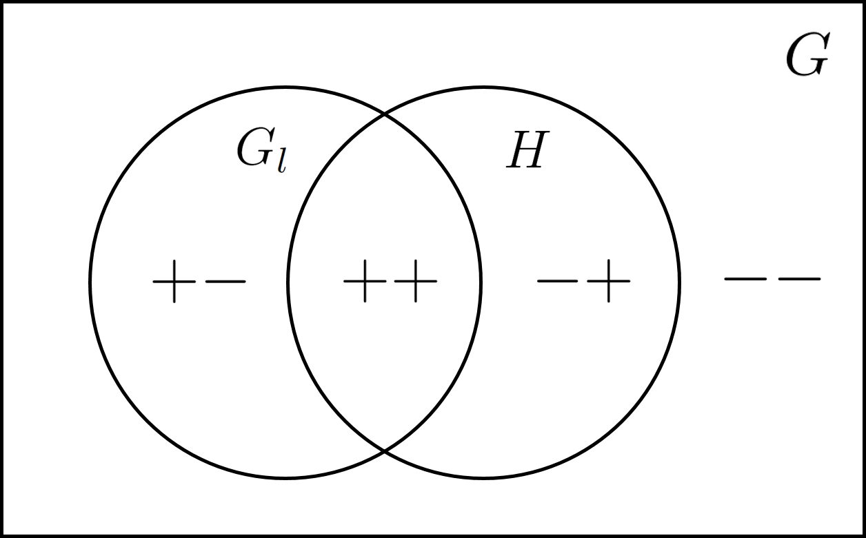
Figure 1: The pattern of symmetry breaking. ($\pm\pm$) denotes boundary conditions of 5D gauge fields.

The gauge fields of the 5-dimensional theory fit into this structure in different ways depending on their UV and IR boundary conditions. We will quote boundary conditions as $+$ or $-$ boundary conditions on $A^{A}_{m}$. Because boundary conditions are imposed on the gauge-covariant $F_{m5}^{A}$,

$$F_{m5}^{A}=\partial_{m}A_{5}^{A}-\partial_{5}A_{m}^{A}+gf^{ABC}A_{m}^{B}A_{5}^{C}\ ,$$ (28)

a $+$ boundary condition for $A_{m}^{A}$ is only consistent with a $-$ boundary condition for $A_{5}^{A}$ and vice versa. In general, a field can have zero modes, zero-energy solutions to the field equations, only with $++$ boundary conditions. Then $A_{m}^{A}$ will have zero modes for $++$ boundary conditions and $A_{5}^{A}$ will have zero modes for $--$ boundary conditions on $A_{m}^{A}$. Zero modes in 5 dimensions are dual to massless particles of the same 4-dimensional spin in 4 dimensions.

These considerations fit together into an appealing picture. Gauge field components with $++$ boundary conditions give massless gauge fields in 4 dimensons. Gauge fields with $--$ boundary conditions give massless scalars in 4 dimensions from $A_{5}^{A}$. These will be Goldstone bosons of the 4-dimensional theory. Coming from the other side of the duality, the underlying gauge symmetries of the 4-dimensional theory can be identified with gauge fields with $+$ UV boundary conditions, while ungauged generators of the global symmetry group are identified with gauge fields with $-$ UV boundary conditions. Global symmetries that are broken at $1/z_{R}$ are identified with gauge fields with $-$ IR boundary conditions, while unbroken global symmetries are identified with gauge fields with $+$ IR boundary conditions. This correspondence, shown also in Fig. 1, precisely identifies $++$ gauge fields with unbroken gauge symmetries and $--$ gauge fields with spontaneously broken global symmetries.

We now have a picture in which Higgs bosons appear as Goldstone bosons of the symmetry breaking in the new strong interaction theory modelled by the 5-dimensional RS fields. This realizes the idea of Higgs fields as Goldstone bosons as proposed in [19] and more recently revived in the “Little Higgs” program [20, 21]. The little hierarchy is produced if the scale of the strong interaction theory, associated with $1/z_{R}$, is much larger than the Higgs field mass and vacuum expectation value. To model this, we take the RS setup as given and generate the Higgs potential from radiative corrections to this picture, described quantitatively by the Coleman-Weinberg potential.

We have presented a formalism for computing the Coleman-Weinberg potential in the previous section. How can a Higgs boson vacuum expectation value be included?

The Higgs bosons appear as zero modes of fields $A_{5}^{A}$. A pure $A^{A}_{5}$ background field can always be removed locally by a gauge transformation. However, in a 5-dimensional system with boundaries, the influence of $A^{A}_{5}(z,x)$ cannot be gauged away completely. There is gauge-invariant information parametrized by the Wilson line

$$W[A]=P\biggl{\{}\exp\bigl{[}ig\int_{z_{0}}^{z_{R}}dz\,A_{5}^{A}T^{A}\bigr{]}\biggr{\}}\ .$$ (29)

The Coleman-Weinberg potential can depend on the Wilson line and, in this way, on the expectation value of $A^{A}_{5}$.

In the formalism of the previous section, the Wilson line appears in the following way: The equations in the previous section apply to free fermion and gauge fields with zero background Higgs fields. We can apply these same formulae to a system with a background $A_{5}^{A}$ field if we gauge away $A_{5}^{A}$ in the central region of $z$, leaving a singular field near $z_{0}$ or $z_{R}$. The effect of a nonzero $A_{5}^{A}$ field is implemented by applying the Wilson line as a matrix to the various fields in the problem, setting $T^{A}=t^{A}$, the representation matrix in the appropriate representation of the gauge group $G$. In this paper, we will generally consider the $A_{5}^{A}$ field as gauged away to the UV boundary. (It is a check on our formalism that the same results can be obtained by gauging away $A_{5}^{A}$ to the IR boundary.)

The zero mode of $A_{5}^{A}$, present when the $A_{m}^{A}$ field has boundary conditions $--$, has the form

$$A_{5}^{A}(z,x^{m})=N_{h}\ z\ h^{A}(x^{m})\ ,$$ (30)

where the $z$ dependence is that of the $A_{5}^{A}$ zero mode and $N_{h}$ is a normalization constant. Then let

$$U_{W}=\exp\bigl{[}-ig\int_{z_{0}}^{z_{R}}dz\,N_{h}z\left\langle{h^{A}}\right\rangle t^{A}\bigr{]}$$ (31)

The matrix $U_{W}$ should be applied to each field before imposing the boundary condition at $z=z_{0}$. In this context, the matrix $U_{W}$ plays the role of the matrix $U$ in (25).

There may be additional complications that influence the UV boundary conditions. For example, it is allowed to introduce a fermion mass term on the boundary,

$$\delta L=\sum_{ij}M_{ij}\overline{\Psi}_{i}\Psi_{j}\ \delta(z-z_{0})\ ,$$ (32)

as long as the mass matrix $M_{ij}$ preserves the assumed local gauge symmetry by mixing only fermion fields with the same $G_{\ell}$ quantum numbers. In this paper, we will include such a mass mixing only on the UV boundary. The effect of this term in models will be to mix fermions actively participating in electroweak symmetry breaking with the light quarks and leptons, similarly to the Extended Technicolor interaction. The influence of (32) is to mix the fermion fields by a unitary transformation. We will implement this directly by including a unitary matrix $U_{M}$ before applying the UV boundary condition.

Our final expression for the matrix ${\bf C}$ is

$${\bf C}=\overrightarrow{B}_{UV}U_{M}U_{W}G\overleftarrow{B}_{IR}\ .$$ (33)

This formula has an important property that we will use often in our discussion. If fermions mixed by $U_{M}$ have the same boundary condition in the UV, then $[U_{M},\overrightarrow{B}_{UV}]=0$. Then we can move $U_{M}$ to the left and find

$$\det{\bf C}=\det U_{M}\cdot\det\biggl{[}\overrightarrow{B}_{UV}U_{W}G\overleftarrow{B}_{IR}\biggr{]}\ .$$ (34)

Since $U_{M}$ is unitary, $\det U_{M}=1$, and the mixing angles in $U_{M}$ disappear from the expression for the Coleman-Weinberg potential. Similarly, if $U_{W}$ mixes only fields with the same IR boundary conditions, we can move $U_{W}$ to the right of $\overleftarrow{B}_{IR}$ and factor it out of determinant calculation. Since $\det U_{W}=1$, the mixing angles in $U_{W}$ do not contribute to the Coleman-Weinberg potential. The Higgs field appears as mixing angles in $U_{W}$ and so, in this latter case, the Coleman-Weinberg potential is flat in $\left\langle{h}\right\rangle$.

This argument extends to decompositions of $U_{W}$ and $U_{M}$: if

$$U_{M}U_{W}=U_{1}U\ \mbox{and}\ [U_{1},\overrightarrow{B}_{UV}]=0$$ (35)

then the Coleman-Weinberg potential does not depend on the angles in $U_{1}$. In moving pieces of the unitary matrix to the right, we must be more careful. The matrix $U_{W}$ mixes fermions within a gauge multiplet, and these must have the same values of $c$, but $U_{M}$ generally mixes fermions in different multiplets with different values of $c$. The fermion Green’s function $G(z_{0},z_{R})$ depends on $c$. So, if

$$U_{W}=UU_{2}\ \mbox{and}\ [U_{2},\overleftarrow{B}_{IR}]=0$$ (36)

then $U_{2}$ does not contribute to the Coleman-Weinberg potential. More generally, pieces of $U_{M}$ may be moved to the right and eliminated if they mix fermion fields with the same value of $c$.

4 Fermion zero modes

Just as the boundary conditions on gauge fields have physical significance, the boundary conditions on fermion fields have a significance for model-building. Five-dimensional fermions are 4-component Dirac fermions, but, with appropriate boundary conditions, they can have zero modes that can be interpreted as chiral quarks and leptons [15, 16].

The zero-mode solutions of the Dirac equation are present for any nonzero value of the 5-dimensional fermion mass. With, again,

$$c=m/k\ ,$$ (37)

a zero mode corresponding to a left-handed 4-dimensional fermion has the form

$$\psi_{L}=f_{-}u_{L}(p)z^{2-c}e^{-ip\cdot x}\qquad\psi_{R}=0\ ,$$ (38)

where $u_{L}(p)$ is the usual 2-component massless spinor of a left-handed fermion and $f_{-}$ is a normalization constant. Similarly, a zero mode corresponding to a right-handed 4-dimensional fermion has the form

$$\psi_{R}=f_{+}u_{R}(p)z^{2+c}e^{-ip\cdot x}\qquad\psi_{L}=0\ .$$ (39)

We will refer to these as $L$ and $R$ zero modes, respectively. These zero modes are nonzero at the boundary, and so they require appropriate fermion boundary conditions, $++$ for the L zero mode and $--$ for the R zero mode.

An important feature of the zero modes is their structure in the 5th dimension. The probability distribution of the position in the 5th dimension is given, for the L zero mode, by

$$\int dz\sqrt{g}\overline{\Psi}(kz\gamma^{0})\Psi=\int dz{kz\over(kz)^{5}}\bigl{|}f_{-}\bigr{|}^{2}z^{4-2c}\sim\int{dz\over z}z^{1-2c}\ .$$ (40)

For $c>\frac{1}{2}$, the zero mode is localized near the UV brane; for $c<\frac{1}{2}$, the zero mode is localized near the IR brane. For the $R$ zero mode, the same calculation gives the boundary at $c=-\frac{1}{2}$. Again,

$$\begin{tabular}[]{lccc}&$c<-\frac{1}{2}$&\quad$-\frac{1}{2}<c<\frac{1}{2}$&\quad$\frac{1}{2}<c$\\ \\ L&IR&\quad IR&\quad UV\\ R&UV&\quad IR&\quad IR\\ \end{tabular}\ .$$ (41)

In a realistic model, the light quarks and leptons would be described by UV zero modes. We will see in a moment that the formation of a symmetry-breaking potential probably requires a pair of IR zero modes which are mixed by a symmetry-breaking Higgs expectation value. The right-handed top quark can potentially be assigned to an IR zero mode. The assignment of the left-handed $(t,b)_{L}$ doublet to IR zero modes is potentially in tension with precision electroweak constraints on the $b_{L}$. This is an important issue for model-building [22].

5 Simplest examples of symmetry breaking

As a first application of this formalism, we review the calculation of the Higgs potential from one fermion multiplet by Contino, Nomura, and Pomarol [12]. We will do this in the simplest context of an $SU(2)$ gauge field acting on two-fermion multiplets. We assign the boundary conditions for the two fermion fields as

$$\Psi\sim\pmatrix{+&+\cr-&-\cr}\ .$$ (42)

The notation here is to write the UV and IR boundary conditions, respectively, for each fermion component on a horizontal line. The matrix represents a single $G$ representation. Fermions in the same $G$ representation must have the same value of $c=m/k$, the parameter that determines the localization of the zero modes. Consistently with these assignments, the gauge fields must be assigned boundary conditions that break $SU(2)$ down to its $U(1)$ subgroup,

$$A^{A}_{m}\sim\pmatrix{-&-\cr-&-\cr+&+\cr}\,$$ (43)

for $A^{1}_{m}$, $A^{2}_{m}$, $A^{3}_{m}$, respectively. Note that, with these assignments, $A_{5}^{1}$ and $A_{5}^{2}$ are Goldstone bosons.

Now turn on $\left\langle{A_{5}^{2}}\right\rangle\neq 0$. This is a direction that breaks the $U(1)$ gauge symmetry and mixes the two fermion components. The corresponding $U_{W}$ is

$$U_{W}=\pmatrix{c_{W}&-s_{W}\cr s_{W}&c_{W}\cr}\ ,$$ (44)

where $c_{W}=\cos\theta$, $s_{W}=\sin\theta$, with

$$\theta={g\over 2}\int_{z_{0}}^{z_{R}}dz\ A_{5}^{2}(z)\ .$$ (45)

Combining (42) and (44), we find the ${\bf C}(p)$ matrix from (24) or (25) as

$${\bf C}=\pmatrix{c_{W}G_{--}&-s_{W}G_{-+}\cr s_{W}G_{+-}&c_{W}G_{++}\cr}\ .$$ (46)

We find immediately

$$\det{\bf C} = c_{W}^{2}G_{--}G_{++}+s_{W}^{2}G_{-+}G_{+-}$$ (47)

$$= (G_{--}G_{++})\biggl{(}1-s_{W}^{2}(G_{--}G_{++}-G_{-+}G_{+-})/G_{--}G_{++}\biggr{)}\ .$$

The first factor is independent of $\theta_{W}$, so we can ignore it. The second factor simplifies with the use of the identity (15), which can be abbreviated here as

$$G_{--}G_{++}-G_{-+}G_{+-}=-{1\over p^{2}z_{0}z_{R}}\ .$$ (48)

We then find

$$\log\det{\bf C}=\log\biggl{[}1+{s_{W}^{2}\over p^{2}z_{0}z_{R}G_{--}\ G_{++}}\biggr{]}\ .$$ (49)

In the Euclidean region, for $z_{0}\ll z_{R}$, all four Green’s functions $G_{--},G_{-+},G_{++},G_{+-}$ are positive definite functions of $p$. All four functions increase exponentially for large $p$, as

$$G_{ab}(z_{0},z_{R})\sim e^{p(z_{R}-z_{0})}\ .$$ (50)

The fermionic contribution to the Coleman-Weinberg potential for this model is then [12]

$$V(h)=-2\int{d^{4}p\over(2\pi)^{4}}\log\biggl{[}1+{s_{W}^{2}\over p^{2}z_{0}z_{R}G_{--}G_{++}}\biggr{]}\ .$$ (51)

This result is well-defined and UV convergent and is negative definite. It is minimized at $\theta=\pi/2$. The depth of the potential depends strongly on the parameter $c$, as shown in Fig. 2. The finiteness of the Coleman-Weinberg potential is an important general feature of gauge-Higgs unification models. It follows from the fact that the Wilson line order parameter of the symmetry breaking is a nonlocal quantity. Since $\left\langle{A_{5}^{A}}\right\rangle$ can be gauged away locally, the potential does not get contributions from the deep ultraviolet. However, the energy scale of the potential is set by $z_{R}$, and so there is still a little hierarchy if $1/z_{R}\gg 100$ GeV.

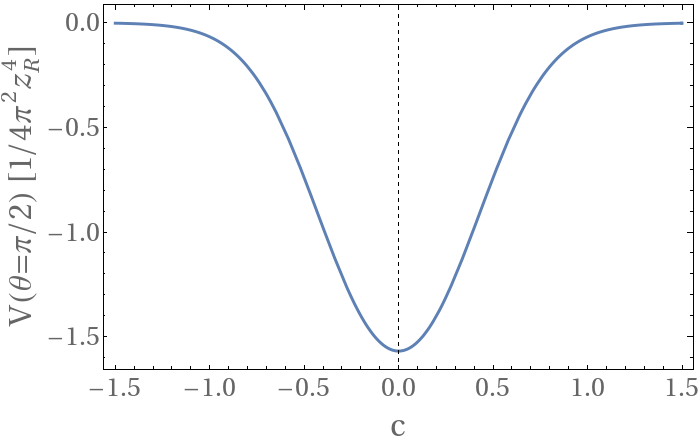
Figure 2: Dependence of the depth of the minimum of the Coleman-Weinberg potential (51) on the parameter $c$.

We must add to the fermion contribution the result for the Coleman-Weinberg potential of the vector bosons. The same formalism applies. The $SU(2)$ gauge group acts on the three gauge boson fields $A^{1}_{M},A^{2}_{M},A^{3}_{M}$ according to

$$t^{a}_{bc}=i\epsilon^{bac}\ .$$ (52)

Then the $U_{W}$ matrix for the three gauge boson states is

$$U_{W}=\pmatrix{c_{2W}&0&s_{2W}\cr 0&1&0\cr-s_{2W}&0&c_{2W}\cr}$$ (53)

where $c_{2W}=\cos 2\theta$, $s_{2W}=\sin 2\theta$, where $\theta$ is as in (45). The boundary conditions on the fields $A_{M}^{1}$ and $A_{M}^{3}$ are the same as those on the two fermion fields in this example. Then we find that the Coleman-Weinberg potential generated by the gauge fields is

$$V(h)=+{3\over 2}\int{d^{4}p\over(2\pi)^{4}}\log\biggl{[}1+{s_{2W}^{2}\over p^{2}z_{0}z_{R}G_{--}G_{++}}\biggr{]}\ .$$ (54)

where, in this expression, $G_{--}$ and $G_{++}$ are evaulated at $c=\frac{1}{2}$.

Some graphs of the complete potential for this model, with $c=\frac{1}{2}$ for the gauge fields and different values of $c$ for the fermions, are shown in Fig 3. In the typical situation, there is a potential barrier between the symmetric point at $h=0$ and the symmetry-breaking minimum; that is, the phase transition is first-order and it is not possible to tune the value of $v/f$ to be small. This is still true if the number of fermion flavors is taken to be a variable $n_{f}$ and varied continuously. The minimum of the potential is always either at $\theta=0$ or $\theta=\pi$.

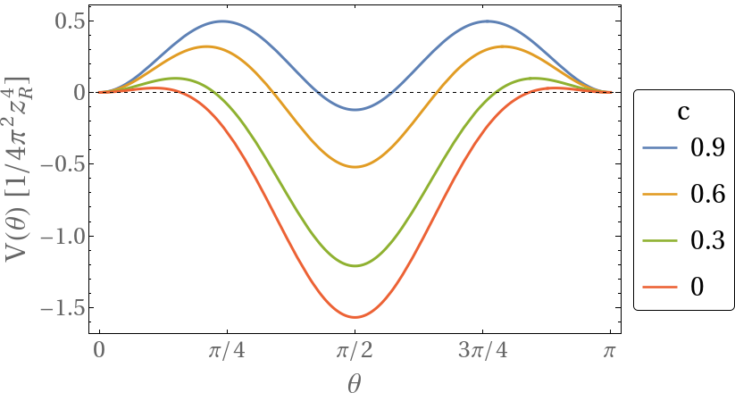
Figure 3: The complete Coleman-Weinberg potential for the model of Section 5, including both fermion and gauge boson contribution.

6 Competing forces with 2 fermion multiplets

To incorporate a little hierarchy with $v/f\ll 1$, a model must be in the vicinity of a second-order phase transition in the space of parameters of the Coleman-Weinberg potential. We would like to understand systematically how to achieve this in models with multiple fermion and gauge fields. In this section, we take a first step into this program by working out the possible phase diagrams of systems of two fermion multiplets. For simplicity, we will restrict ourselves to $SU(2)$ in this section, and we will ignore the gauge field contributions to the potential. We call the two fermion multiplets $\psi_{1}$ and $\psi_{2}$ and assign them mass parameters $c_{1}$ and $c_{2}$. We will call the Green’s functions associated with these multiplets $G^{1}_{ab}$ and $G^{2}_{ab}$, respectively. An example of the full expansion of this notation is

$$G^{1}_{+-}=G^{(\psi_{1})}_{+-}(z_{0},z_{R})\ .$$ (55)

6.1 No UV mixing

Consider first the simplest case in which there is no UV mass mixing ($U_{M}={\bf 1}$). In this case, we have a pair of fermion representations in the 2 of $SU(2)$, with boundary conditions such as

$$\pmatrix{+&+\cr-&-\cr}\qquad\pmatrix{+&-\cr-&-\cr}$$ (56)

In Appendix A, we show that the reversal of the $c$ parameter and the UV and IR boundary conditions

$$c\to-c\ ,\qquad+\leftrightarrow-$$ (57)

is a symmetry of a free fermion in RS. According to the argument given below (34), a fermion multiplet gives zero contribution to the Coleman-Weinberg potential if either its two UV boundary conditions or its two IR boundary conditions are identical. Then, for one fermion multiplet, there are only two possible situation in which we obtain a nonzero Coleman-Weinberg potential

$$\psi_{A}\sim\pmatrix{+&+\cr-&-\cr}\qquad\mbox{and}\qquad\psi_{R}\sim\pmatrix{+&-\cr-&+\cr}\ .$$ (58)

We call these the A (“attractive”) and R (“repulsive”) cases, respectively.

The potential in the attractive case was worked out in (51) above. For future reference, we notate this potential as a function of $s_{W}=\sin\theta$ and the fermion mass parameter $c$,

$$V_{A}(s_{W},c)=-2\int{d^{4}p\over(2\pi)^{4}}\log\biggl{[}1+{s_{W}^{2}\over p^{2}z_{0}z_{R}G_{--}G_{++}}\biggr{]}\ .$$ (59)

The potential is negative definite, and its minimum is always at $s_{W}=1$.

The potential in the repulsive case can be worked out in the same way. From

$${\bf C}=\pmatrix{c_{W}G_{-+}&-s_{W}G_{--}\cr s_{W}G_{++}&c_{W}G_{+-}\cr}\ ,$$ (60)

we find using the same method

$$V_{R}(s_{W},c)=-2\int{d^{4}p\over(2\pi)^{4}}\log\biggl{[}1-{s_{W}^{2}\over p^{2}z_{0}z_{R}G_{-+}G_{+-}}\biggr{]}\ .$$ (61)

This potential is positive definite, and its minimum is always at $s_{W}=0$. One way to understand its repulsive nature is that here the Higgs expectation value mixes two massive states and therefore lowers the mass of the lightest state. This is energetically less favored, so the potential resists forming a condensate.

If we have two fermion multiplets, one with the A type and one with the R type boundary conditions, these two multiplets will compete. To understand the competition, we need to work out the expansions of $V_{A}$ and $V_{R}$ about $s_{W}=0$. This is done in Appendix D. These expressions have expansions in $\sin\theta$ with the forms

$$V_{A}(s_{W},c) = {1\over 4\pi^{2}z_{R}^{4}}\left[-A_{A}(c)s_{W}^{2}+{1\over 2}B_{A}(c)s_{W}^{4}+{1\over 2}C_{A}(c)s_{W}^{4}\log(1/s_{W}^{2})+{\cal O}(s_{W}^{6})\right]$$

$$V_{R}(s_{W},c) = {1\over 4\pi^{2}z_{R}^{4}}\left[+A_{R}(c)s_{W}^{2}+{1\over 2}B_{R}(c)s_{W}^{4}+{\cal O}(s_{W}^{6})\right]\ ,$$ (62)

where we have chosen the signs so that all of the coefficients are positive functions of $c$. Fig. 4 shows that $A_{A}(c)>A_{R}(c)$, but both functions are rapidly decreasing functions of $c$. Then there is a line in the $(c_{1},c_{2})$ plane, shown as a dotted line in Fig. 5, where

$$A_{A}(c_{1})=A_{R}(c_{2})\ .$$ (63)

For $c_{1}$ slightly outside this boundary, the potential $V_{A}(c_{1})+V_{R}(c_{2})$ has a negative quadratic term in $s_{W}$ that goes to zero on the curve (63), and a positive quartic term. Then the curve (63) is a line of second-order transitions. Near this line, the minimum $v$ of the potential can be made as small as we like. For the representative case $z_{0}/z_{R}=0.01$, the tip of the curve occurs with $c_{2}=0$ at $c_{1}=0.2997$.

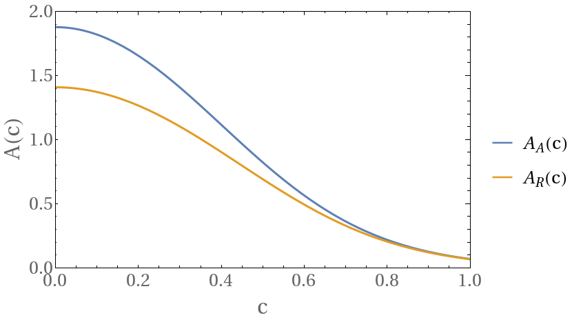
Figure 4: The $c$-dependence of $A_{A}(c)$ and $A_{R}(c)$.

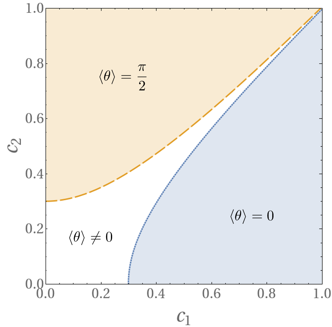
Figure 5: Phase diagram of the model of Section 6.1 in the $c_{1}-c_{2}$ plane. In most values of $c_{1}$ and $c_{2}$, the minimum is at either $\left\langle{\theta}\right\rangle=0$ or $\left\langle{\theta}\right\rangle=\pi/2$. However, a non-trivial minimum is realized in the middle white area. Note that along the line $c_{1}=c_{2}$, $\left\langle{\theta}\right\rangle=\pi/4$.

Actually, there are two minima, at $v$ and $-v$. These minima merge to a single minimum at $\left\langle{\theta}\right\rangle=\pi/2$ along the line of bifurcations indicated by the dashed line in Fig 5.

6.2 Cases with UV mixing

In the remainder of this section, we will extend this analysis to the more general case of two $SU(2)$ fermion multiplets with mass mixing on the UV brane. We will analyze the cases systematically for all possible choices of fermion boundary conditions. It is interesting, at least to us, that all of the cases that we will encounter can be understood from the competition between attractive and repulsive boundary conditions that we have seen already in Section 6.1. That is, this concept is robust with respect to turning on fermion mixing on the UV boundary. In most cases, the generalization is relatively straightforward, although the last case considered in Section 6.6 has some nontrivial features.

A given fermion multiplet has $2^{4}$ possible boundary conditions, so a pair of multiplets has $256$ different boundary conditions to analyze. However, many of these are related by the symmetry $+\leftrightarrow-$, $c\leftrightarrow-c$ or by interchange of the top and bottom components of the fermion multiplets. Also, as we showed at the end of Section 3, mass mixing on the UV brane has physical effect only if the fermions mixed by the mass term have different UV boundary conditions. The strategy of our analysis will be to enumerate the different possible IR boundary conditions and then to go through the 16 cases of UV boundary conditions from the simplest to the most difficult, using symmetries whereever possible to reduce cases to equivalent ones.

The 16 possible IR boundary conditions can be reduced to four cases. Case I includes the two cases

$$\pmatrix{\phantom{+}&+\cr\phantom{+}&+\cr} \pmatrix{\phantom{+}&+\cr\phantom{+}&+\cr}$$

$$\pmatrix{\phantom{+}&+\cr\phantom{+}&+\cr} \pmatrix{\phantom{+}&-\cr\phantom{+}&-\cr}$$ (64)

and two more cases with $+\leftrightarrow-$. Case II includes the eight cases equivalent to

$$\pmatrix{\phantom{+}&+\cr\phantom{+}&-\cr}\qquad\pmatrix{\phantom{+}&+\cr\phantom{+}&+\cr}$$ (65)

Case III includes

$$\pmatrix{\phantom{+}&+\cr\phantom{+}&-\cr}\qquad\pmatrix{\phantom{+}&-\cr\phantom{+}&+\cr}$$ (66)

and the equivalent case with $+\leftrightarrow-$. Case IV includes

$$\pmatrix{\phantom{+}&+\cr\phantom{+}&-\cr}\qquad\pmatrix{\phantom{+}&+\cr\phantom{+}&-\cr}$$ (67)

and the equivalent case with $+\leftrightarrow-$.

For each case, we have 16 choices of UV boundary conditions. We will also introduce mixing by angles $\alpha$ between the two fermions in the top row and $\beta$ between the two fermions in the bottom row. In cases in which the two multiplets have the same boundary conditions, such as

$$\pmatrix{+&\phantom{+}\cr-&\phantom{+}\cr}\qquad\pmatrix{+&\phantom{+}\cr-&\phantom{+}\cr}$$ (68)

the mixing can be removed. In cases such as

$$\pmatrix{+&\phantom{+}\cr-&\phantom{+}\cr}\qquad\pmatrix{-&\phantom{+}\cr-&\phantom{+}\cr}\qquad\mbox{and}\qquad\pmatrix{-&\phantom{+}\cr-&\phantom{+}\cr}\qquad\pmatrix{+&\phantom{+}\cr-&\phantom{+}\cr}$$ (69)

the mixing by $\beta$ has no effect but the potential depends on the mixing angle $\alpha$. Actually, the two cases shown in (69) are equivalent, since increasing $\alpha$ by $\pi/2$ interchanges the two boundary conditions in the top line. So, for each case listed above, we have a trivial situation in which the potential is independent of $\alpha$ and $\beta$, situations in which the potential only depends on one angle, and one case of the greatest complexity in which the potential depends on both angles.

6.3 Case I

In case I, the IR boundary conditions are the same for both fermions in each multiplet. Then, by the argument at the end of Section 3, the Coleman-Weinberg potential is independent of $s_{W}$. For all of these cases,

$$V(s_{W},c_{1},c_{2})=0\ .$$ (70)

6.4 Case II

For case II, we begin from the IR boundary conditions in (65) and add UV boundary conditions, for which there are 16 possibilities. These can be grouped into three sets.

In the first set (4 cases), the UV boundary conditions are the same between the two multiplets, and the calculation of the Coleman-Weinberg potential reduces to that of two separate multiplets. For example, in

$$\pmatrix{+&+\cr-&-\cr}\qquad\pmatrix{+&+\cr-&+\cr}$$ (71)

the second multiplet gives zero and the combined potential is obviously

$$V(s_{W},c_{1},c_{1})=V_{A}(s_{W},c_{1})\ .$$ (72)

All of these cases give a potential equal to either $V_{A}(s_{W},c)$ or $V_{R}(s_{W},c)$.

In the second set, with one pair of UV boundary conditions identical, there are 8 cases, connected in pairs by $\alpha\to\alpha+\pi/2$ or $\beta\to\beta+\pi/2$. An example is

$$\pmatrix{+&+\cr+&-\cr}\qquad\pmatrix{-&+\cr+&+\cr}\ ,$$ (73)

for which the potential depends on $\alpha$ but not on $\beta$. In addition, the contribution to the potential from $\psi_{2}$ has no dependence on $s_{W}$. We can thus reduce the unitary transformation at the UV brane to

$$U=\pmatrix{c_{\alpha}&0&-s_{\alpha}&0\cr 0&1&0&0\cr s_{\alpha}&0&c_{\alpha}&0\cr 0&0&0&1\cr}\pmatrix{c_{W}&-s_{W}&0&0\cr s_{W}&c_{W}&0&0\cr 0&0&1&0\cr 0&0&0&1\cr}=\pmatrix{c_{\alpha}c_{W}&-c_{\alpha}s_{W}&-s_{\alpha}&0\cr s_{W}&c_{W}&0&0\cr s_{\alpha}c_{W}&-s_{\alpha}s_{W}&c_{\alpha}&0\cr 0&0&0&1\cr}\ ,$$ (74)

where $c_{\alpha}=\cos\alpha$, $s_{\alpha}=\sin\alpha$. The matrix ${\bf C}$ then has the form

$${\bf C}=\pmatrix{c_{\alpha}c_{W}G^{1}_{--}&-c_{\alpha}s_{W}G^{1}_{-+}&-s_{\alpha}G^{2}_{--}&0\cr s_{W}G^{1}_{--}&c_{W}G^{1}_{-+}&0&0\cr s_{\alpha}c_{W}G^{1}_{+-}&-s_{\alpha}s_{W}G^{1}_{++}&c_{\alpha}G^{2}_{+-}&0\cr 0&0&0&G^{2}_{--}\cr}\ .$$ (75)

It is easy to check that $\det U=1$. The cancellations in that calculation guide the simplification of $\det{\bf C}$. We find

$$\det{\bf C} = (c_{\alpha}^{2}G^{1}_{--}G^{2}_{+-}+s_{\alpha}^{2}G^{1}_{+-}G^{2}_{--})G^{1}_{-+}G^{2}_{--}$$ (76)

$$\hskip 14.45377pt+s_{\alpha}^{2}s_{W}^{2}(G^{2}_{--})^{2}(G^{1}_{--}G^{1}_{++}-G^{1}_{-+}G^{1}_{+-})\ .$$

We can reduce the last term using the Wronskian identity (15) and extract a factor independent of $s_{W}^{2}$. Then the Coleman-Weinberg potential becomes

$$V(s_{W},c_{1},c_{2})=-2\int{d^{4}p\over(2\pi)^{4}}\log\biggl{[}1-{s_{\alpha}^{2}s_{W}^{2}\over p^{2}z_{0}z_{R}G^{1}_{-+}G^{1}_{+-}}{1\over(s_{\alpha}^{2}+c_{\alpha}^{2}G^{1}_{--}G^{2}_{+-}/G^{2}_{--}G^{1}_{+-})}\biggr{]}\ .$$ (77)

This is a purely repulsive potential with strength diminished by $s_{\alpha}^{2}$. In fact, for $c_{1}=c_{2}$,

$$V(s_{W},c_{1},c_{2})=V_{R}(s_{\alpha}s_{W},c_{1})\ .$$ (78)

A way to guess the answer (78) is to note that, for $s_{\alpha}=0$, there is no mixing and the potential can be seen by inspection to be zero, while for $s_{\alpha}=1$, the UV boundary conditions $+$ and $-$ in the top lines of (73) are reversed and the potential is exactly that of the repulsive case in Section 6.1.

The other three similar cases can be analyzed in the same way. They are either purely attractive or purely repulsive. We quote the results for the potential in the case $c_{1}=c_{2}$:

$$\pmatrix{+&+\cr-&-\cr}\quad\pmatrix{-&+\cr-&+\cr}\quad\to\quad V = V_{A}(c_{\alpha}s_{W},c_{1})$$

$$\pmatrix{+&+\cr+&-\cr}\quad\pmatrix{+&+\cr-&+\cr}\quad\to\quad V = V_{A}(s_{\beta}s_{W},c_{1})$$

$$\pmatrix{-&+\cr+&-\cr}\quad\pmatrix{-&+\cr-&+\cr}\quad\to\quad V = V_{R}(c_{\beta}s_{W},c_{1})\ .$$ (79)

Finally, we come to the case in which the potential depends on both mixing angles

$$\pmatrix{+&+\cr+&-\cr}\quad\pmatrix{-&+\cr-&+\cr}\ .$$ (80)

For this case, $U_{M}$ depends on both $\alpha$ and $\beta$, but we can still simplify $U_{W}$ as in (74), so that

$$U=\pmatrix{c_{\alpha}c_{W}&-c_{\alpha}s_{W}&-s_{\alpha}&0\cr c_{\beta}s_{W}&c_{\beta}c_{W}&0&-s_{\beta}\cr s_{\alpha}c_{W}&-s_{\alpha}s_{W}&c_{\alpha}&0\cr s_{\beta}s_{W}&s_{\beta}c_{W}&0&c_{\beta}\cr}\ .$$ (81)

The corresponding ${\bf C}$ matrix is

$${\bf C}=\pmatrix{c_{\alpha}c_{W}G^{1}_{--}&-c_{\alpha}s_{W}G^{1}_{-+}&-s_{\alpha}G^{2}_{--}&0\cr c_{\beta}s_{W}G^{1}_{--}&c_{\beta}c_{W}G^{1}_{-+}&0&-s_{\beta}G^{2}_{--}\cr s_{\alpha}c_{W}G^{1}_{+-}&-s_{\alpha}s_{W}G^{1}_{++}&c_{\alpha}G^{2}_{+-}&0\cr s_{\beta}s_{W}G^{1}_{+-}&s_{\beta}c_{W}G^{1}_{++}&0&c_{\beta}G^{2}_{+-}\cr}\ .$$ (82)

Then

$$\det{\bf C} = c_{\alpha}^{2}c_{\beta}^{2}G^{1}_{--}G^{1}_{-+}(G^{2}_{+-})^{2}+c_{\alpha}^{2}s_{\beta}^{2}G^{1}_{--}G^{1}_{++}G^{2}_{--}G^{2}_{+-}$$ (83)

$$+s_{\alpha}^{2}c_{\beta}^{2}G^{1}_{+-}G^{1}_{-+}G^{2}_{--}G^{2}_{+-}+s_{\alpha}^{2}s_{\beta}^{2}G^{1}_{+-}G^{1}_{++}(G^{2}_{--})^{2}$$

$$-(s_{\alpha}^{2}c_{\beta}^{2}-s_{\beta}^{2}c_{\alpha}^{2})s_{W}^{2}G^{2}_{--}G^{2}_{+-}/p^{2}z_{0}z_{R}\ .$$

We then find

$$V=-2\int{d^{4}p\over(2\pi)^{4}}\log\biggl{[}1-{s_{-}s_{+}s_{W}^{2}\over p^{2}z_{0}z_{R}{\bf D}}\biggr{]}\ ,$$ (84)

where

$$s_{-}=\sin(\alpha-\beta)\qquad s_{+}=\sin(\alpha+\beta)$$ (85)

and

$${\bf D}=c_{\alpha}^{2}c_{\beta}^{2}G^{1}_{--}G^{1}_{-+}{G^{2}_{+-}\over G^{2}_{--}}+c_{\alpha}^{2}s_{\beta}^{2}G^{1}_{--}G^{1}_{++}+s_{\alpha}^{2}c_{\beta}^{2}G^{1}_{+-}G^{1}_{-+}+s_{\alpha}^{2}s_{\beta}^{2}G^{1}_{+-}G^{1}_{++}{G^{2}_{--}\over G^{2}_{+-}}$$ (86)

is a positive definite factor. This potential switches from repulsive to attractive according to the sign of $s_{-}s_{+}$. In the repulsive case, the minimum is at $s_{W}=0$, in the attractive case, the minimum is at $s_{W}=1$, so there is no interesting competition here that allows Higgs vacuum expectation value to be arbitrarily small.

6.5 Case III

For case III, we begin with the IR boundary conditions in (66) and add UV boundary conditions, covering the same 16 possibilities as in the previous section.

As in the previous section, the first four cases, with equal boundary conditions in the UV for both fermion multiplets, have potentials independent of $\alpha$ and $\beta$. The cases with all $+$ and all $-$ boundary conditions in the UV give potentials equal to zero. The case

$$\pmatrix{+&+\cr-&-\cr}\qquad\pmatrix{+&-\cr-&+\cr}$$ (87)

gives

$$V(s_{W},c_{1},c_{2})=V_{A}(s_{W},c_{1})+V_{R}(s_{W},c_{2})\ ,$$ (88)

precisely the case with competition analyzed in Section 6.1. The last case

$$\pmatrix{-&+\cr+&-\cr}\qquad\pmatrix{-&-\cr+&+\cr}$$ (89)

gives a similar result.

The next set of cases have a potential that depends on one but not both mixing angles. The first example is

$$\pmatrix{+&+\cr+&-\cr}\qquad\pmatrix{-&-\cr+&+\cr}\ .$$ (90)

It is straightforward to work out the potential using the methods already described. We have

$${\bf C}=\pmatrix{c_{\alpha}c_{W}G^{1}_{--}&-c_{\alpha}s_{W}G^{1}_{-+}&-s_{\alpha}c_{W}G^{2}_{-+}&s_{\alpha}s_{W}G^{2}_{--}\cr s_{W}G^{1}_{--}&c_{W}G^{1}_{-+}&0&0\cr s_{\alpha}c_{W}G^{1}_{+-}&-s_{\alpha}s_{W}G^{1}_{++}&c_{\alpha}c_{W}G^{2}_{++}&-c_{\alpha}s_{W}G^{2}_{+-}\cr 0&0&s_{W}G^{2}_{-+}&c_{W}G^{2}_{--}\cr}\ .$$ (91)

Computing the determinant and assembling the Coleman-Weinberg potential, we find

$$V=-2\int{d^{4}p\over(2\pi)^{4}}\log\biggl{[}1+{s_{W}^{2}\over p^{2}z_{0}z_{R}}{c_{\alpha}^{2}G^{1}_{--}G^{1}_{-+}-s_{\alpha}^{2}G^{2}_{--}G^{2}_{-+}\over{\bf D}}\biggr{]}\ ,$$ (92)

where now

$${\bf D}=c_{\alpha}^{2}G^{1}_{--}G^{1}_{-+}G^{2}_{--}G^{2}_{++}+s_{\alpha}^{2}G^{2}_{--}G^{2}_{-+}G^{1}_{-+}G^{1}_{+-}\ .$$ (93)

This potential interpolates between the attractive case, for $s_{\alpha}=0$, and the repulsive case, for $s_{\alpha}=1$. However, for almost all values of $s_{\alpha}$, the potential is monotonic and so is minimized at $s_{W}=0$, for smaller values of $s_{\alpha}$ or at $s_{W}=1$, for larger values of $s_{\alpha}$. To understand this better, examine the first two derivatives of (92). These are

$${\partial V\over\partial(s_{W}^{2})}\biggr{|}_{0} = -2\int{d^{4}p\over(2\pi)^{4}}\ \biggl{[}{1\over p^{2}z_{0}z_{R}}{c_{\alpha}^{2}G^{1}_{--}G^{1}_{-+}-s_{\alpha}^{2}G^{2}_{--}G^{2}_{-+}\over{\bf D}}\biggr{]}$$

$${\partial^{2}V\over\partial(s_{W}^{2})^{2}}\biggr{|}_{0} = +2\int{d^{4}p\over(2\pi)^{4}}\ \biggl{[}{1\over p^{2}z_{0}z_{R}}{c_{\alpha}^{2}G^{1}_{--}G^{1}_{-+}-s_{\alpha}^{2}G^{2}_{--}G^{2}_{-+}\over{\bf D}}\biggr{]}^{2}\ .$$ (94)

The $s_{W}^{4}$ is always positive, but, when the $s_{W}^{2}$ term vanishes, the $s_{W}^{4}$ term has almost the same zero and is doubly suppressed. Thus, this case has a second order phase transition where the vacuum expectation value of the Higgs field goes to zero, but it occurs only in an extremely fine-tuned interval of $s_{\alpha}$.

The other three cases in which $V$ depends on one mixing angle are related to this case by exchanging $+\leftrightarrow-$ boundary conditions and exchanging the two fermion multiplets, by interchanging top and bottom within each representation and sending $\alpha\to\beta+\pi/2$, or by both of these operations. All four cases then have the behavior just described.

The remaining cases with this choice of IR boundary condition can all be described as cases of

$$\pmatrix{+&+\cr+&-\cr}\qquad\pmatrix{-&-\cr-&+\cr}$$ (95)

with arbitrary values of the mixing angles $\alpha$ and $\beta$. We can get a feeling for the result by considering the special cases: (a) For $\alpha=\beta=0$, the value of the Coleman-Weinberg potential is zero; (b) if $\alpha=\pi/2$, $\beta=0$, then both fermions are in the repulsive case, (c) if $\alpha=0$, $\beta=\pi/2$, both fermions are in the attractive case. Then there will be no competition between the two representations, but the minimum of the potential will swing back and forth between $s_{W}=0$ and $s_{W}=1$ according to the values of $\alpha$ and $\beta$.

The precise form of the potential can be worked out as in the previous cases. The result is

$$V=-2\int{d^{4}p\over(2\pi)^{4}}\log\biggl{[}1-{s_{W}^{2}\over p^{2}z_{0}z_{R}}{s_{-}s_{+}(G^{1}_{--}G^{1}_{++}+G^{2}_{-+}G^{2}_{+-})\over{\bf D}}-{s^{2}_{W}c_{W}^{2}\over(p^{2}z_{0}z_{R})^{2}}{s_{-}^{2}\over{\bf D}}\biggr{\}}\biggr{]}\ ,$$ (96)

with $s_{-}$, $s_{+}$ as in (85) and where now

$${\bf D} = c_{\alpha}^{2}c_{\beta}^{2}G^{1}_{--}G^{1}_{-+}G^{2}_{+-}G^{2}_{++}+c_{\alpha}^{2}s_{\beta}^{2}G^{1}_{--}G^{1}_{++}G^{2}_{--}G^{2}_{++}$$ (97)

$$+s_{\alpha}^{2}c_{\beta}^{2}G^{1}_{-+}G^{1}_{+-}G^{2}_{-+}G^{2}_{+-}+s_{\alpha}^{2}s_{\beta}^{2}G^{1}_{+-}G^{1}_{++}G^{2}_{--}G^{2}_{-+}\ .$$

Note that, using (48),

$$G^{1}_{--}G^{1}_{++}+G^{2}_{-+}G^{2}_{+-}=G^{1}_{-+}G^{1}_{+-}+G^{2}_{--}G^{2}_{++}\ ,$$ (98)

so (96) has the required symmetry between $\psi_{1}$ and $\psi_{2}$. This potential has just the form described in the previous paragraph, with zeros along lines where $s_{-}=\sin(\alpha-\beta)=0$.

6.6 Case IV

For case IV, we begin with the IR boundary conditions in (67) and add UV boundary conditions, covering the same 16 possibilities as in the previous section.

The cases with both UV boundary conditions equal is again trivial, giving potentials equal to $0$, $0$, $V_{A}(s_{W},c_{1})+V_{A}(s_{W},c_{2})$, and $V_{R}(s_{W},c_{1})+V_{R}(s_{W},c_{2})$ in the four cases.

The first case with one mixing angle is

$$\pmatrix{+&+\cr+&-\cr}\qquad\pmatrix{-&+\cr+&-\cr}\ .$$ (99)

For $\alpha=0$, we have zero for the potential from $\psi_{1}$ and the repulsive case $V_{R}(s_{W},c_{2})$ from $\psi_{2}$. For $\alpha=\pi/2$, the potential from $\psi_{1}$ is in the repulsive case $V_{R}(s_{W},c_{1})$ and the potential from $\psi_{2}$ is zero. This suggests that the potential is always repulsive, with its minimum at $s_{W}=0$. The precise form of the potential is

$$V=-2\int{d^{4}p\over(2\pi)^{4}}\log\biggl{[}1-{s_{W}^{2}\over p^{2}z_{0}z_{R}}{c_{\alpha}^{2}G^{1}_{--}G^{1}_{-+}+s_{\alpha}^{2}G^{2}_{--}G^{2}_{-+}\over{\bf D}}\biggr{]}\ ,$$ (100)

with

$${\bf D}=c_{\alpha}^{2}G^{1}_{--}G^{1}_{-+}G^{2}_{-+}G^{2}_{+-}+s_{\alpha}^{2}G^{1}_{-+}G^{1}_{+-}G^{2}_{--}G^{2}_{-+}\ .$$ (101)

This expression is clearly positive definite, with a zero at $s_{W}=0$. The second case with one mixing angle

$$\pmatrix{+&+\cr-&-\cr}\qquad\pmatrix{-&+\cr-&-\cr}$$ (102)

is similarly always in the attractive case, with its minimum at $s_{W}=1$. The full expression for the potential is

$$V=-2\int{d^{4}p\over(2\pi)^{4}}\log\biggl{[}1+{s_{W}^{2}\over p^{2}z_{0}z_{R}}{c_{\alpha}^{2}G^{2}_{+-}G^{2}_{++}+s_{\alpha}^{2}G^{1}_{+-}G^{1}_{++}\over{\bf D}}\biggr{]}\ ,$$ (103)

with

$${\bf D}=c_{\alpha}^{2}G^{1}_{--}G^{1}_{++}G^{2}_{+-}G^{2}_{++}+s_{\alpha}^{2}G^{1}_{+-}G^{1}_{++}G^{2}_{--}G^{2}_{++}\ .$$ (104)

The remaining two cases are related to these by reversing the top and bottom rows.

The final case, with dependence on two mixing angles, is

$$\pmatrix{+&+\cr+&-\cr}\qquad\pmatrix{-&+\cr-&-\cr}\ .$$ (105)

The Coleman-Weinberg potential can be worked out as above; the result is

$$V=-2\int{d^{4}p\over(2\pi)^{4}}\log\biggl{[}1+{s_{W}^{2}\over p^{2}z_{0}z_{R}}{s_{-}s_{+}(G^{1}_{++}G^{1}_{--}-G^{2}_{++}G^{2}_{--})\over{\bf D}}+{s^{2}_{W}c_{W}^{2}\over(p^{2}z_{0}z_{R})^{2}}{s_{-}^{2}\over{\bf D}}\biggr{\}}\biggr{]}\ ,$$ (106)

with $s_{-}$, $s_{+}$ as in (85) and where now

$${\bf D} = c_{\alpha}^{2}c_{\beta}^{2}G^{1}_{--}G^{1}_{-+}G^{2}_{+-}G^{2}_{++}+c_{\alpha}^{2}s_{\beta}^{2}G^{1}_{--}G^{1}_{++}G^{2}_{+-}G^{2}_{-+}$$ (107)

$$+s_{\alpha}^{2}c_{\beta}^{2}G^{1}_{+-}G^{1}_{-+}G^{2}_{--}G^{2}_{++}+s_{\alpha}^{2}s_{\beta}^{2}G^{1}_{+-}G^{1}_{++}G^{2}_{--}G^{2}_{-+}\ .$$

The form of this expression shows explicit competition between $\psi_{1}$ and $\psi_{2}$. Most of this can be understood by considering limit points where the two fermions decouple from one another: at $\alpha=0$, $\beta=0$, both fermions have potential equal to zero; at $\alpha=\pi/2$, $\beta=0$, $\psi_{1}$ is in the repulsive case while $\psi_{2}$ is in the attractive case; at $\alpha=0$, $\beta=\pi/2$, $\psi_{1}$ is in the attractive case while $\psi_{2}$ is in the repulsive case.

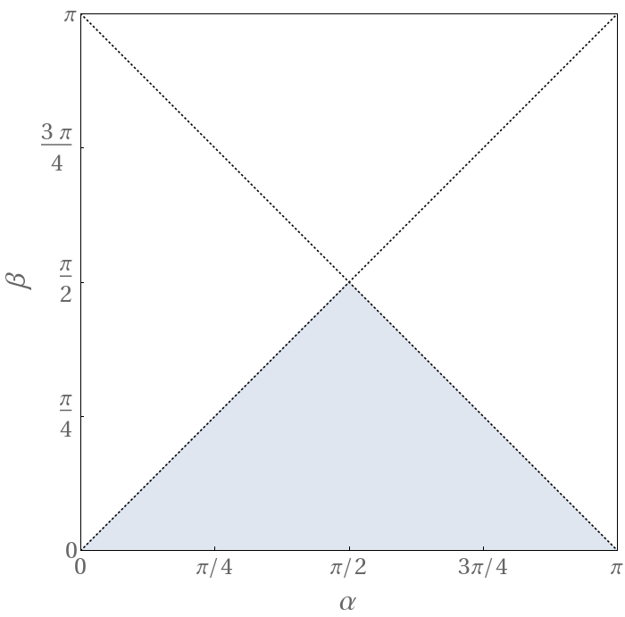
Figure 6: Fundamental region of the $(\alpha,\beta)$ plane useful for describing the phase diagram of the model (105).

To understand the full dynamics of this model, it is useful to reduce it to the minimal region of the $(\alpha,\beta)$ plane. The potential (106) depends only on $s_{-}s_{+}$ and $s_{-}^{2}$. Then the potential takes the same value under the translations

$$\alpha\to\alpha+\pi,\ \beta\to\beta\quad\mbox{and}\quad\alpha\to\alpha,\ \beta\to\beta+\pi\ .$$ (108)

and under the reflection

$$\alpha\to-\alpha,\ \beta\to-\beta$$ (109)

This implies that the fundamental region for $(\alpha,\beta)$ is the triangle

$$0<\alpha<\pi,\ 0<\beta<\pi,\ \alpha+\beta<\pi\ .$$ (110)

Further, reflection across the line $\alpha-\beta=0$, that is,

$$\alpha\leftrightarrow\beta\ ,$$ (111)

changes the sign of the competition term in (106) and so is equivalent to interchanging $\psi_{1}$ and $\psi_{2}$. The full dynamics of the model is then exhibited in the triangle shown in Fig. 6, with $\psi_{1}$ always in the repulsive case and $\psi_{2}$ always in the attractive case.

The phase diagram shown in Fig. 5 changes smoothly with $\alpha$ and $\beta$ across this diagram. Note that, while the coefficient of $s_{W}^{2}$ in $V(s_{W})$ can have either sign, the coefficient of $s_{W}^{4}$ is always positive. Then we will find a line of second-order phase transitions where $\partial V/\partial(s_{W}^{2})$ is zero. At the bottom center of the triangle, $\alpha=\pi/2$, $\beta=0$, we have a case equivalent to that of Section 6.1. There is a curve of second-order phase transitions with its tip at $c_{1}=0$, $c_{2}=0.2997$ (for $z_{0}/z_{R}=0.01$). Across the bottom of the triangle, the critical value of $c_{2}$ for $c_{1}=0$ increases slowly from 0.2697 at $\alpha=0$ to 0.2997 at $\alpha=\pi/2$ and back to 0.2697 at $\alpha=\pi$.

The other two edges of the triangle have simple forms for $V(s_{W})$. Along the line $\alpha=\beta$, $V(s_{W})=0$. Along the line $\alpha+\beta=\pi$, $s_{+}=0$ and so the potential takes the simple attractive form

$$V=-2\int{d^{4}p\over(2\pi)^{4}}\log\biggl{[}1+{s^{2}_{W}c_{W}^{2}\over(p^{2}z_{0}z_{R})^{2}}{s_{-}^{2}\over{\bf D}}\biggr{]}\ ,$$ (112)

with minima at $s_{W}^{2}=c_{W}^{2}=\frac{1}{2}$. In accordance with this, the critical value of $c_{2}$ at $c_{1}=0$ varies along each horizontal line with fixed $\beta>0$, tending to 0 as the left-hand boundary is approached and to $\infty$ as the right-hand boundary is approached. The critical value at $\alpha=\pi/2$ remains close to 0.3 for all values of $\beta$.

7 An example with relaxed fine-tuning

We have now seen that the examples of the previous section can all be understood in terms of the competition of fermion multiplets with attractive and repulsive boundary conditions. However, the only cases with a large $v/f$ hierarchy were those in which the values of the parameters $c_{1}$ and $c_{2}$ were adjusted to be close to a line of second-order phase transitions. In other words, the Coleman-Weinberg potential that we have encountered so far is always strongly attractive or repulsive. In most of the parameter space, the value of of $v/f$ was not affected by the competition, and the potential was minimized at $s_{W}=0$ or at $s_{W}=1$.

More quantitatively, among the terms in the potential expansion (62), the quadratic term $s_{W}^{2}$ almost always dominates over the quartic term $s_{W}^{4}$ and therefore the overall sign of $s_{W}^{2}$ simply determines the vacuum. For a non-trivial minimum, the parameters $c_{1}$ and $c_{2}$ should be fine-tuned so that the overall strength of $s_{W}^{2}$ becomes smaller than that of $s_{W}^{4}$. This implies that for a natural explanation of a large $v/f$ hierarchy, a weakly repulsive fermion is required, which contributes to the Higgs potential only at the quartic level without the quadratic term.

Here is an example: Consider a fermion multiplet in the triplet representation of $SU(2)$ with boundary conditions

$$\psi_{3}\sim\pmatrix{q_{+}\cr q_{0}\cr q_{-}\cr}\sim\pmatrix{+&-\cr-&-\cr-&+\cr}\ ,$$ (113)

where $(q_{+},q_{0},q_{-})$ are eigenstates of the generator $t^{3}$. If the Goldstone boson $\left\langle{A_{5}^{2}}\right\rangle$ connected the two fermions $q_{+}$ and $q_{-}$, the triplet would generate a repulsive potential. However, the form of the generator is

$$t^{2}={1\over\sqrt{2}}\pmatrix{0&-i&0\cr i&0&-i\cr 0&i&0\cr}\ ,$$ (114)

and it only connects $q_{+}\leftrightarrow q_{0}$ and $q_{0}\leftrightarrow q_{-}$. Then the Coleman-Weinberg potential must be flat in the $t^{2}$ direction, at least in the leading order. The same applies to $\left\langle{A_{5}^{1}}\right\rangle$. Indeed, the matrix $U_{W}$ acting on $\psi_{3}$ has the form

$$U_{W}=\pmatrix{c^{2}_{W}&-s_{2W}/\sqrt{2}&s^{2}_{W}\cr s_{2W}/\sqrt{2}&c_{2W}&-s_{2W}/\sqrt{2}\cr s^{2}_{W}&s_{2W}/\sqrt{2}&c^{2}_{W}\cr}\ ,$$ (115)

where $s_{2W}=\sin 2\theta_{W}$. The Coleman-Weinberg potential from this multiplet is

$$V_{3}(s_{W},c)=-2\int{d^{4}p\over(2\pi)^{4}}\log\biggl{[}1-{s_{W}^{4}\over p^{2}z_{0}z_{R}G_{-+}G_{+-}}\biggr{]}\ .$$ (116)

This potential has no $s_{W}^{2}$ term and is repulsive in quartic order. Fig. 7 shows the shape of the three potentials $V_{A},V_{R},V_{3}$ near $s_{W}=0$, all for $c=0$. We can see $V_{3}$ is indeed only weakly repulsive.

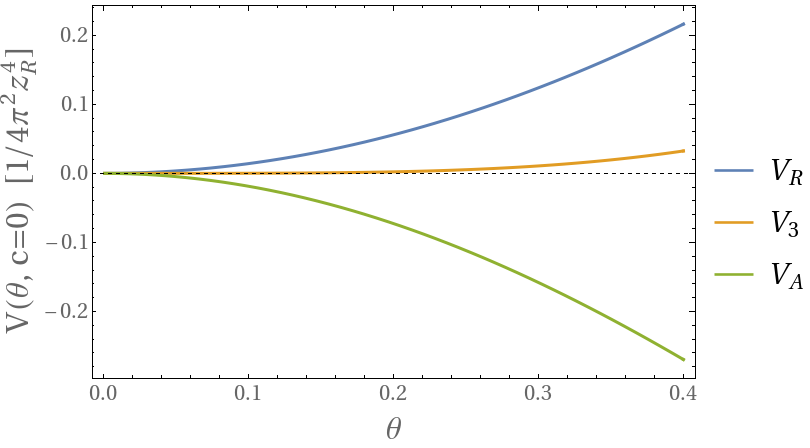
Figure 7: The shape of $V_{A},V_{R},V_{3}$ near $s_{W}=0$. All three potentials are for $c=0$.

To study the effect of the new triplet $\psi_{3}$ on the phase diagram, first consider a system with two fermion multiplets, an attractive doublet $\psi_{A}$ and the triplet $\psi_{3}$. Fig. 8 shows the minimum $\left\langle{\theta}\right\rangle$ of the Coleman-Weinberg potential as a function of $c_{1}$ with $c_{3}=0$ fixed. This theory is always in the broken phase $s_{W}>0$, as it must be, but for $c_{1}>0.3$ the large contribution to the quartic term from $\psi_{3}$ multiplet pushes the minimum of the potential to small values.

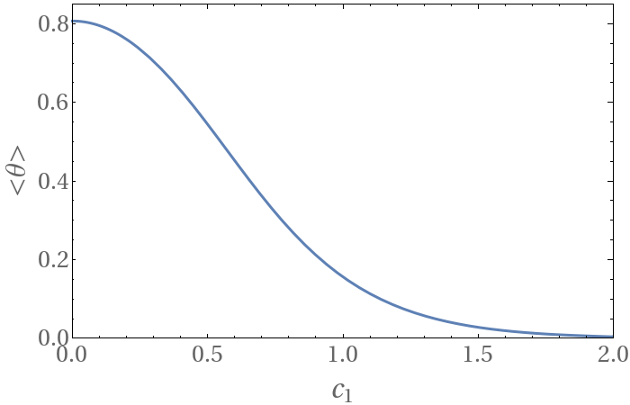
Figure 8: The minimum of the potential $V_{A}(s_{W},c_{1})+V_{3}(s_{W},c_{3}=0)$, shown as a function of $c_{1}$.

More generally, we can use the multiplet $\psi_{3}$ to lower the degree of fine-tuning needed to achieve a small value of $v/f$ in a system with competition between attractive and repulsive fermion multiplets. Consider a model with $\psi_{A}$ and $\psi_{R}$ fermions as in Section 6.1, and add the multiplet $\psi_{3}$. The position of the line of phase transitions does not change, since $\psi_{3}$ contributes only quartic terms, but the presence of the quartic term from $\psi_{3}$ can expand the region where $v/f$ is small. In Fig. 9, we vary the parameter $c_{3}$ from high values to $c_{3}=0$ and show the values of $c_{1}$ and $c_{2}$ for which $\left\langle{s_{W}^{2}}\right\rangle=0.01$, a value sought in realistic RS models. The vertical axis is a measure of the fine-tuning needed to achieve $v/f\ll 1$.

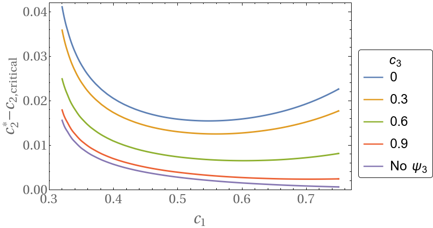
Figure 9: Separation of $c_{2}^{*}$ from its critical value $c_{2,critical}$ on the line of phase transition corresponding to $\left\langle{\theta}\right\rangle=0.1$. These values are shown as a function of $c_{1}$, where the lowest curve has the $\psi_{3}$ omitted (or $c_{3}\to\infty$) and the highest curve has $c_{3}=0$.

It is interesting that the multiplet $\psi_{3}$ includes a right-handed zero mode. By coupling it weakly to other fermions through boundary conditions at $z_{0}$, we can give this fermion a small mass without disrupting the Coleman-Weinberg potential. An interesting possibility for a realistic model is then to introduce right-handed quarks and leptons in the weakly repulsive multiplets and connect them at the UV boundary to the left-handed doublets. This will generate fermion masses much smaller than the top quark mass while simultaneously making a $v/f$ hierarchy more natural.

8 Conclusions

In this paper, we reviewed the formalism for fermions and gauge fields in the RS geometry and the potential for fermion condensation. We presented a simple formula, implementing ideas of Falkowski, for computing the Coleman-Weinberg potential for the Higgs field. Using this formula, we explored the idea of competition between fermion multiplets with different boundary conditions and presented strategies for achieving the hierarchy $v/f\ll 1$ needed in realistic models.

We hope that these tools will be useful for the construction of realistic RS models with bulk fermions and gauge fields which could provide predictive models of strongly coupled Higgs bosons. In a forthcoming paper, we will apply the methods discussed here to an illustrative models of electroweak symmetry breaking driven by top quark condensation [8].

Appendix A Basic formalism for fermions in RS

In this appendix, we present details of our formalism for fermion fields in RS. We begin in Minkowski space. Capital letters denote 5-dimensional indices, taking the values 0,1,2,3,5, with $M,N,\ldots$ for world indices and $A,B,\ldots$, for tangent-space indices. Lower-case letters denote 4-dimensional indices. We use the metric (2). After deriving the equations of motion, and after gauge fixing in the case of vector bosons, we go to Euclidean space by the continuation $p^{0}\to ip^{0}$, $p^{2}\to-p^{2}$.

The Dirac action in RS is

$$S=\int d^{4}xdz\biggl{(}\sqrt{-g}\ \overline{\Psi}\bigl{[}ie^{M}_{A}\gamma^{A}{\cal D}_{M}-m\bigr{]}\Psi-\overline{\cal K}\Psi-\overline{\Psi}{\cal K}\biggr{)}\ ,$$ (117)

where ${\cal D}_{M}$ is the gravity- and gauge-covariant derivative and $e^{M}_{A}=kz\delta^{M}_{A}$ for the metric (2). We denote the gauge-covariant derivative as $D_{M}$; then ${\cal D}_{M}=D_{M}+\frac{1}{2}\omega_{M}{}^{AB}\Sigma_{AB}$. The nonzero terms in the spin connection are

$$\omega_{m}{}^{a5}=-\omega_{m}{}^{5a}={1\over z}\delta^{a}_{m}\ .$$ (118)

We divide the 4-component Diract field $\Psi$ into two 2-component fields as in (4),

$$\Psi=\pmatrix{\psi_{L}\cr\psi_{R}\cr}\ ,$$ (119)

using the basis of Dirac matrices

$$\gamma^{a}=\pmatrix{&\sigma^{a}\cr\overline{\sigma}^{a}&\cr}\ \ \mbox{and}\ \ \gamma^{5}=-i\Gamma\equiv-i\pmatrix{-1&\cr&1\cr}\ .$$ (120)

The matrix $\Gamma$ denotes the 4-dimensional chirality. With these conventions, the Dirac action takes the form

$$S = \int d^{4}xdz\biggl{(}{1\over(kz)^{4}}\biggl{[}\psi^{\dagger}_{L}i\overline{\sigma}^{m}D_{m}\psi_{L}+\psi^{\dagger}_{R}i\sigma^{m}D_{m}\psi_{R}$$ (121)

$$\hskip 14.45377pt+\psi^{\dagger}_{L}\bigl{(}D_{5}-{2\over z}-{c\over z}\bigr{)}\psi_{R}+\psi^{\dagger}_{R}\bigl{(}-D_{5}+{2\over z}-{c\over z}\bigr{)}\psi_{L}\biggr{]}-\overline{\cal K}\Psi-\overline{\Psi}{\cal K}\biggr{)}\ .$$

Let

$${\bf D}=D_{5}-{2+c\over z}\ ,\qquad\overline{\bf D}=D_{5}-{2-c\over z}\ .$$ (122)

Then the homogeneous equations of motion for $\Psi$ are

$${1\over(kz)^{4}}\pmatrix{-\overline{\bf D}&i\sigma^{m}D_{m}\cr i\overline{\sigma}^{m}D_{m}&{\bf D}\cr}\pmatrix{\psi_{L}\cr\psi_{R}\cr}=0\ .$$ (123)

In gauge-Higgs unification, we assume that the background gauge field has the form

$$A_{M}^{a}=(0,0,0,0,A_{5}^{a}(z))$$ (124)

In this case, we can Fourier analyze in the 4 extended dimensions, so that $i\overline{\sigma}^{m}D_{m}\to\overline{\sigma}\cdot p$, $i\sigma^{m}D_{m}\to\sigma\cdot p$. Then we see that these fields obey

$$\Delta_{\Psi}(p^{2})\Psi\equiv{1\over(kz)^{4}}\pmatrix{-\overline{\bf D}&\sigma\cdot p\cr\overline{\sigma}\cdot p&{\bf D}\cr}\pmatrix{\psi_{L}\cr\psi_{R}\cr}=0$$ (125)

The contribution of a fermion to the Coleman-Weinberg potential is then

$$V_{\Psi}=-\int{d^{4}p\over(2\pi)^{4}}\log\det\Delta_{\Psi}(-p^{2})\ .$$ (126)

This is the precise expression for the $\det(\Psi)$ term in (10).

We can eliminate either $\psi_{L}$ or $\psi_{R}$ from (125). Once this is done, the remaining field obeys

$$\Delta_{L}(p^{2})\psi_{L}\equiv\bigl{(}p^{2}+{\bf D}\overline{\bf D}\bigr{)}\psi_{L} = 0$$

$$\Delta_{R}(p^{2})\psi_{R}\equiv\bigl{(}p^{2}+\overline{\bf D}{\bf D}\bigr{)}\psi_{R} = 0$$ (127)

Up to possible contributions from zero modes, $\Delta_{L}(p^{2})$ and $\Delta_{R}(p^{2})$ have the same spectrum. The operators $\Delta_{L}(p^{2})$ and $\Delta_{R}(p^{2})$ include no spin matrices and can be thought of as applied to single-component fields. Then we can rewrite the Coleman-Weinberg potential as

$$V_{\Psi}=-2\int{d^{4}p\over(2\pi)^{4}}\log\det\Delta_{L}(-p^{2})=-2\int{d^{4}p\over(2\pi)^{4}}\log\det\Delta_{R}(-p^{2})\ .$$ (128)

The factor 2 counts the 2 spin degrees of freedom. This is the more precise expression for the $\det(\Psi)$ term in (10).

For $A_{5}(z)=0$, the homogeneous equations (127) are solved by

$$\psi_{L}\sim z^{5/2}(J_{c+1/2}(pz),Y_{c+1/2}(pz))\qquad\psi_{R}\sim z^{5/2}(J_{c-1/2}(pz),Y_{c-1/2}(pz))\ .$$ (129)

Standard identities for Bessel functions imply that these solutions are interchanged by ${\bf D}$ and $\overline{\bf D}$, when $A_{5}(z)=0$. For example,

$$\overline{\bf D}(z^{5/2}J_{c+1/2}(pz)) = p\,(z^{5/2}J_{c-1/2}(pz))$$

$${\bf D}(z^{5/2}J_{c-1/2}(pz)) = -p\,(z^{5/2}J_{c+1/2}(pz))\ .$$ (130)

To calculate the Coleman-Weinberg potential, we must continue these equations to Euclidean space. The continuation of (125) is

$$\Delta_{\Psi}\Psi\equiv{1\over(kz)^{4}}\pmatrix{-\overline{\bf D}&i\sigma\cdot p\cr i\overline{\sigma}\cdot p&{\bf D}\cr}\pmatrix{\psi_{L}\cr\psi_{R}\cr}=0$$ (131)

where now $\sigma\cdot p=p^{0}+i\vec{\sigma}\cdot\vec{p}$, $\overline{\sigma}\cdot p=p^{0}-i\vec{\sigma}\cdot\vec{p}$. The operators ${\bf D}$, $\overline{\bf D}$ have the action on the $G$ functions (12)

$$\overline{\bf D}_{z}\,z^{5/2}G_{+\beta}(z,z^{\prime})=pz^{5/2}G_{-\beta}(z,z^{\prime})\qquad{\bf D}_{z}\,z^{5/2}G_{-\beta}(z,z^{\prime})=-pz^{5/2}G_{+\beta}(z,z^{\prime})\ .$$ (132)

The field $\Psi$ has four Green’s functions,

$${\cal G}_{LL}(z,z^{\prime},p)=\left\langle{\psi_{L}(p,z)\psi_{R}^{\dagger}(-p,z^{\prime})}\right\rangle {\cal G}_{LR}(z,z^{\prime},p)=\left\langle{\psi_{L}(p,z)\psi_{L}^{\dagger}(-p,z^{\prime})}\right\rangle$$

$${\cal G}_{RL}(z,z^{\prime},p)=\left\langle{\psi_{R}(p,z)\psi_{R}^{\dagger}(-p,z^{\prime})}\right\rangle {\cal G}_{RR}(z,z^{\prime},p)=\left\langle{\psi_{R}(p,z)\psi_{L}^{\dagger}(-p,z^{\prime})}\right\rangle$$ (133)

which are interconnected through the equations

$$\Delta_{\Psi}{\cal G}(z,z^{\prime},p)=\delta(z-z^{\prime}){\bf 1}$$ (134)

and similar equations with operators applied to the right and acting on $z^{\prime}$. If the fermion field has multiple gauge components $\Psi^{A}$, these equations become matrix equations. For example, ${\cal G}^{AB}_{LL}$ will have the form

$${\cal G}_{LL}^{AB}(z,z^{\prime},p) = p^{2}z_{R}k^{4}(zz^{\prime})^{5\over 2}[{\bf A}^{AB}G^{(A)}_{+,-A_{R}}(z,z_{R})G^{(B)}_{-,-B_{R}}(z^{\prime},z_{R})$$ (135)

$$\hskip-36.135pt-\cases{\delta^{AB}A_{R}G^{(A)}_{+,A_{R}}(z,z_{R})G^{(A)}_{-,-A_{R}}(z^{\prime},z_{R})]&$z<z^{\prime}$\cr\delta^{AB}A_{R}G^{(A)}_{+,-A_{R}}(z,z_{R})G^{(A)}_{-,A_{R}}(z^{\prime},z_{R})]&$z>z^{\prime}$\cr}\ .$$

In this equation, $A_{R}$ represents the boundary condition of the field $A$ at $z=z_{R}$. That is, $A_{R}=+$ if the field $A$ has $+$ boundary condition on IR brane, and $A_{R}=-$ if otherwise. $A_{R}=\pm$ implies $-A_{R}=\mp$. In the second line, $A_{R}$ denotes a factor $\pm 1$ depending on the sign of $A_{R}$. We can obtain ${\cal G}^{AB}_{LR}$, ${\cal G}^{AB}_{RL}$, and ${\cal G}^{AB}_{RR}$, using (134), the similar equation acting on $z^{\prime}$, and (132). In particular, ${\cal G}^{AB}_{RR}(z,z^{\prime})$ has the same form with the first indices of the $G$ functions reversed $+\leftrightarrow-$ from (135).

Because $\psi_{L}$ and $\psi_{R}$ are interconnected, it is not consistent to place separate boundary conditions on these fields. Instead, it is sufficient to place the boundary conditions

$$+\ :\ \ \psi_{R}=0\quad\mbox{or}\quad-\ :\ \ \psi_{L}=0$$ (136)

A zero mode in $\psi_{L}$ requires $(++)$ boundary conditions; a zero mode in $\psi_{R}$ requires $(--)$ boundary conditions.

Note that the equations for $L$ and $R$ are interchanged by the interchange of boundary conditions $+\leftrightarrow-$ and the interchange ${\bf D}\leftrightarrow\overline{\bf D}$, or equivalently, $c\leftrightarrow-c$. After these two interchanges, the fermion field will have the same functional determinant.

Appendix B Basic formalism for gauge fields in RS

In this appendix, we present details of our formalism for gauge fields in RS. Conventions for the 5-dimensional space are as in Appendix A.

The gauge field action in RS is

$$S=\int d^{4}xdz\ \biggl{(}\sqrt{-g}\biggl{[}-{1\over 4}g^{MP}g^{NQ}F^{a}_{MN}F^{a}_{PQ}\biggr{]}-{\cal J}^{M}A_{M}\biggr{)}\ .$$ (137)

In our formalism, the Higgs field is a background gauge field, so we will quantize in the Feynman-Randall-Schwartz background field gauge [17]. Expand

$$A_{M}^{a}\to A_{M}^{a}(z)+{\cal A}_{M}^{a}\ ,$$ (138)

where, on the right, $A_{M}^{a}$ is a fixed background field,

$$A_{M}^{a}=(0,0,0,0,A_{5}^{a}(z))$$ (139)

as in (124), and ${\cal A}_{M}^{a}$ is a fluctuating field. Let $A_{M}=A_{M}^{a}t^{a}$ and $F_{MN}=F^{a}_{MN}t^{a}$, where $t^{a}$ are the generators of the gauge group, and let $D_{M}$ be the covariant derivative containing the background field only. Then the linearized form for the field strength is

$$F_{MN}=D_{M}{\cal A}_{N}-D_{N}{\cal A}_{M}\ .$$ (140)

After inserting the metric (2) and performing some integrations by parts, the linearized gauge action becomes

$$S = \int d^{4}xdz\ \biggl{(}\frac{1}{2}{1\over kz}\biggl{[}{\cal A}^{n}D^{m}D_{m}{\cal A}_{n}-{\cal A}_{m}D^{n}D^{m}{\cal A}_{n}-{\cal A}^{n}kzD_{5}{1\over kz}D_{5}A_{n}$$ (141)

$$\hskip 28.90755pt-{\cal A}_{5}D^{m}D_{m}{\cal A}_{5}+2{\cal A}_{5}D^{m}D_{5}{\cal A}_{m}\biggr{]}-{\cal J}^{m}{\cal A}_{m}+{\cal J}_{5}{\cal A}_{5}\biggr{)}\ .$$

Here and in the following, raised and lowered indices are contracted with the Lorentz metric $\eta^{mn}$. Following [17], introduce the gauge-fixing term

$$S_{GF}=\int d^{4}xdz{1\over(kz)^{5}}\biggl{[}-{1\over 2\xi}\biggl{(}(kz)^{2}D^{m}{\cal A}_{m}-\xi(kz)^{3}D_{5}{1\over kz}{\cal A}_{5}\biggr{)}^{2}\biggr{]}\ .$$ (142)

Then

$$S+S_{GF} = \int d^{4}xdz\ \biggl{(}\frac{1}{2}{1\over kz}\biggl{[}{\cal A}_{m}\bigl{(}\eta^{mn}D^{2}-\eta^{mn}kzD_{5}{1\over kz}D_{5}-D^{m}D^{n}(1-{1\over\xi})\bigr{)}{\cal A}_{n}$$ (143)

$$\hskip 28.90755pt+{\cal A}_{5}\bigl{(}-D^{2}+\xi D_{5}kzD_{5}{1\over kz}\bigr{)}{\cal A}_{5}\biggr{]}-{\cal J}^{m}{\cal A}_{m}+{\cal J}_{5}{\cal A}_{5}\biggr{)}\ .$$

The linearized ghost action is

$$S_{ghost}=\int d^{4}xdz\ \biggl{(}{1\over kz}\biggl{[}\overline{c}\bigl{(}-D^{2}+\xi kzD_{5}{1\over kz}D_{5}\bigr{)}c\biggr{]}-\overline{\cal C}c-\overline{c}{\cal C}\biggr{)}\ .$$ (144)

These formulae simplify for $\xi=1$. The homogeneous equations for the gauge field components are

$$\Delta_{G}(p^{2}){\cal A}_{m}(z,p) \equiv {1\over kz}\bigl{(}p^{2}+zD_{5}{1\over z}D_{5}\bigr{)}{\cal A}_{m}(z,p)=0$$

$$\Delta_{5}(p^{2}){\cal A}_{5}(z,p) \equiv {1\over kz}\bigl{(}p^{2}+D_{5}zD_{5}{1\over z}\bigr{)}{\cal A}_{5}(z,p)=0$$

$$\Delta_{c}(p^{2})c(z,p) \equiv {1\over kz}\bigl{(}p^{2}+zD_{5}{1\over z}D_{5}\bigr{)}c(z,p)=0\ .$$ (145)

Up to possible contributions from zero modes, $\Delta_{G}(p^{2})$, $\Delta_{5}(p^{2})$ and $\Delta_{c}(p^{2})$ have the same spectrum for consistent boundary conditions, as defined below. Then when we integrate out the fields ${\cal A}_{m}$, $A_{5}$, and $(c,\overline{c})$ we find

$$(\det\Delta_{G})^{4/2}(\det\Delta_{5})^{1/2}(\det\Delta_{c})^{-1}=(\det\Delta_{G})^{3/2}\ .$$ (146)

The contribution of a gauge boson to the Coleman-Weinberg potential is then

$$V_{G}=+{3\over 2}\int{d^{4}p\over(2\pi)^{4}}\log\det\Delta_{G}(-p^{2})\ .$$ (147)

This is the precise expression for the $\det(A)$ term in (10). The operators $\Delta_{G}$, $\Delta_{5}$ are related to the operators $\Delta_{L}$, $\Delta_{R}$ defined in (127) for fermion fields with $c=\frac{1}{2}$, by

$$\Delta_{L}=z^{3/2}(kz\Delta_{G}){1\over z^{3/2}}\qquad\Delta_{R}=z^{3/2}(kz\Delta_{5}){1\over z^{3/2}}\ .$$ (148)

Thus, the calculation of the determinant of $\Delta_{G}$ and $\Delta_{5}$ for gauge fields are special cases of the determinant calculation for fermion fields.

For $A_{5}(z)=0$, the homogeneous equations (145) are solved by

$$A_{m}\ ,\ c\sim z^{1}(J_{1}(pz),Y_{1}(pz))\qquad A_{5}\sim z^{1}(J_{0}(pz),Y_{0}(pz))\ .$$ (149)

Standard identities for Bessel functions imply that these solutions are interchanged by the action of $\partial_{5}$ and $kz\partial_{5}(1/kz)$.

The Green’s functions for gauge fields are

$$\left\langle{{\cal A}_{m}(z,p){\cal A}_{n}(z^{\prime},-p)}\right\rangle = \eta_{mn}{\cal G}(z,z^{\prime},p)$$

$$\left\langle{{\cal A}_{5}(z,p){\cal A}_{5}(z^{\prime},-p)}\right\rangle = {\cal G}_{5}(z,z^{\prime},p)$$

$$\left\langle{c(z,p)\overline{c}(z^{\prime},-p)}\right\rangle = {\cal G}_{c}(z,z^{\prime},p)\ .$$ (150)

These satisfy the differential equations in $z$

$$\Delta_{G}(p^{2}){\cal G}(z,z^{\prime},p) = \delta(z-z^{\prime})$$

$$\Delta_{5}(p^{2}){\cal G}_{5}(z,z^{\prime},p) = \delta(z-z^{\prime})$$

$$\Delta_{c}(p^{2}){\cal G}_{c}(z,z^{\prime},p) = \delta(z-z^{\prime})\ .$$ (151)

The solutions to the gauge field equations are interrelated by

$${\cal A}_{5}(z)=D_{5}{\cal A}_{m}(z)\qquad{\cal A}_{m}(z)=kzD_{5}{1\over kz}{\cal A}_{5}\ .$$ (152)

These transformations interchange the boundary conditions

$$+\ :\ \ D_{5}{\cal A}_{m}(z)=0 -\ :\ \ {\cal A}_{m}(z)=0$$

$$-\ :\ \ {\cal A}_{5}(z)=0 +\ :\ \ kzD_{5}({1\over kz}{\cal A}_{5}(z))=0$$

If ${\cal A}_{m}(z)$ is assigned the boundary condition $+$ (respectively, $-$), then consistently ${\cal A}_{5}(z)$ must be assigned the boundary condition $-$ (respectively, $+$).

Appendix C Proof of Falkowski’s Theorem

In this appendix, we provide a proof of Falkowski’s Theorem (27) by explicit calculation of $A_{5}$ tadpole diagrams. In Appendices A and B, we have obtained the operators $\Delta_{\Psi}$, $\Delta_{G}$, $\Delta_{5}$ and $\Delta_{c}$ from the quadratic Lagrangian for fermion and gauge fields under the background field

$$A_{M}^{a}=(0,0,0,0,A_{5}^{a}(z))\ .$$ (154)

Then, the effective potential from each field can be written as the functional determinant of the corresponding operator.

In this derivation, we will turn on the gauge field $A_{5}^{a}$ along a fixed direction in the adjoint representation. Then we will simplify by writing $A_{5}^{a}t^{a}=A_{5}t$. It will be important to remember that, while the mixing matrix $U_{M}$ in (33) can mix fermion fields in a more arbitrary way, the matrices $t$ and $U_{W}$ can only connect fermions in the same gauge representations, which must therefore have the same value of $c$. (For gauge bosons, always $c=\frac{1}{2}$.) If $t$ is proportional to the unit matrix, it generates a pure phase in $U_{W}$. This affects the determinant of ${\bf C}$, but such a phase manifestly cancels out of the equation (22) and so has no effect on ${\bf A}$. In the proof of the theorem below, we can then assume that $t$ generates no overall phase,

$$\sum_{AB}t_{AB}\delta^{AB}=0\ .$$ (155)

Consider first the fermion case

$$V_{\Psi}=-\int{d^{4}p\over(2\pi)^{4}}\log\det\Delta_{\Psi}\ .$$ (156)

where $p$ is the 4d Euclidean momentum. Varying $A_{5}(z)$, we find

$$\delta V_{\Psi} = -\int{d^{4}p\over(2\pi)^{4}}\ {\mbox{\rm tr}}\left[\Delta_{\Psi}^{-1}{\delta\Delta_{\Psi}}\right]$$

$$= -\int{d^{4}p\over(2\pi)^{4}}\int_{z_{0}}^{z_{R}}dz\ {\mbox{\rm tr}}\left[{\cal G}(z,z){1\over(kz)^{4}}(-ig\Gamma\delta A_{5}(z)t)\right]$$

$$= -\int{d^{4}p\over(2\pi)^{4}}\int_{z_{0}}^{z_{R}}dz(-ig\delta A_{5}(z))\ {\mbox{\rm tr}}\left[{1\over(kz)^{4}}(-{\cal G}_{LL}(z,z)+{\cal G}_{RR}(z,z))t\right]\ .$$

We can obtain the Green’s function by gauging $A_{5}$ away to the UV boundary, as explained in the Section 3. The full Green’s function is related to the Green’s function for $A_{5}(z)=0$ by

$${\cal G}(z,z^{\prime})=\exp[-ig\int^{z_{R}}_{z}d\overline{z}A_{5}(\overline{z})t]\ {\cal G}_{0}(z,z^{\prime})\ \exp[+ig\int^{z_{R}}_{z^{\prime}}d\overline{z}A_{5}(\overline{z})t]\ .$$ (158)

In our method of turning on $A_{5}$, this field is essentially Abelian, and the exponential factors cancel out for $z=z^{\prime}$. Then we can use the expression of the Green’s function from (135) to evaluate (LABEL:arrangeV). The trace part within the integrand becomes

$${\cal T} = {1\over(kz)^{4}}{\mbox{\rm tr}}\left[(-{\cal G}_{LL}(z,z)+{\cal G}_{RR}(z,z))t\right]$$ (159)

$$= 2p^{2}zz_{R}\sum_{A,B}t_{BA}{\bf A}^{AB}$$

$$\hskip 14.45377pt(-G^{(A)}_{+,-A_{R}}(z,z_{R})G^{(B)}_{-,-B_{R}}(z,z_{R})+G^{(A)}_{-,-A_{R}}(z,z_{R})G^{(B)}_{+,-B_{R}}(z,z_{R}))\ .$$

The factor 2 comes from the trace over spinor indices. Note that the terms with $\delta^{AB}$ in ${\cal G}^{AB}_{LL}(z,z)$ and ${\cal G}^{AB}_{RR}(z,z)$ are identical in the symmetric limit $z\to z^{\prime}$ and cancel each other. Here and in the rest of this appendix, summation over field indices $A$, $B$. etc. is always explicitly shown.

From (24), we have

$${\bf C}_{AC}=(U_{M}U_{W})_{AC}\,G^{(C)}_{-A_{0},-C_{R}}\ .$$ (160)

Using (22) and (135), we can formally solve for ${\bf A}^{AB}$,

$${\bf A}^{AB}=\sum_{C,D}({\bf C}^{-1})_{AC}(U_{M}U_{W})_{CD}D_{R}\delta^{DB}G^{(D)}_{-C_{0},+B_{R}}\ .$$ (161)

In last line of (159), the states $A$ and $B$ are connected by $t_{BA}$. Then these states have the same value of $c$, and so we can use (48) to evaluate the expression in parentheses,

$$\hskip-57.81621pt(-G^{(A)}_{+,-A_{R}}(z,z_{R})G^{(B)}_{-,-B_{R}}(z,z_{R})+G^{(A)}_{-,-A_{R}}(z,z_{R})G^{(B)}_{+,-B_{R}}(z,z_{R}))$$ (162)

$$= \cases{0&$A_{R}=B_{R}$\cr-1/p^{2}zz_{R}&$A_{R}=+$, $B_{R}=-$\cr+1/p^{2}zz_{R}&$A_{R}=-$, $B_{R}=+$\cr}$$

$$= (B_{R}\delta_{A_{R},-B_{R}})/p^{2}zz_{R}$$

Assembling the pieces,

$${\cal T} = 2\sum_{A,B,C}({\bf C}^{-1})_{AC}((U_{M}U_{W})_{CB}B_{R}G^{(B)}_{-C_{0},+B_{R}})\ t_{BA}\ (B_{R}\delta_{A_{R},-B_{R}})$$ (163)

$$= 2\sum_{A,B,C}\bigl{(}({\bf C}^{-1})_{AC}\ (U_{M}U_{W})_{CB}G^{(B)}_{-C_{0},-A_{R}}\bigr{)}\ t_{BA}\ \delta_{A_{R},-B_{R}}\ .$$

The two factors of $B_{R}$ cancel, and then we are very close to the desired form.

There is one further issue: The sum in (159) is taken only over pairs $(A,B)$ such that $A_{R}=-B_{R}$. We would like to extend this to a sum over all pairs. To do this, use the identity ${\bf C}^{-1}{\bf C}={\bf 1}$. Writing this out using (160), we have

$$\sum_{C}({\bf C}^{-1})_{AC}(U_{M}U_{W})_{CB}G^{(B)}_{-C_{0},-B_{R}}=\delta_{AB}$$ (164)

For $(A,B)$ such that $A_{R}=B_{R}$, this has the same form as the summand of (163). For $A\neq B$, (164) is zero and we can add these terms to (163). For $A=B$, for which necessarily $A_{R}=B_{R}$, the trace of this identity with $t_{AB}$ is $\delta_{AB}t_{AB}=0$, and so we can also add back those terms. Then there is no change in (163) if we extend the sum to all pairs $(A,B)$.

Finally, we find

$$\delta V_{\Psi} = -2\int{d^{4}p\over(2\pi)^{4}}\ \sum_{A,B,C}({\bf C}^{-1})_{AC}(U_{M}U_{W})_{CB}\left(-ig\int dz\delta A_{5}(z)t\right)_{BA}G^{(B)}_{-C_{0},-A_{R}}$$ (165)

$$= -2\int{d^{4}p\over(2\pi)^{4}}\ \sum_{A,B,C}{\bf C}^{-1}_{AC}\ \delta{\bf C}_{CA}$$

$$= -2\int{d^{4}p\over(2\pi)^{4}}\ \delta\log\det{\bf C}$$

Integrating up from $A_{5}(z)=0$, we obtain the contribution of a fermion to the Coleman-Weinberg potential

$$V_{\Psi}=-2\int{d^{4}p\over(2\pi)^{4}}\log\det{\bf C}(p)$$ (166)

up to an additive, $A_{5}$-independent constant. This completes the proof of Falkowski’s Theorem for the fermion determinants.

In (148), we pointed out that the evaluations of the gauge boson determinants were special cases of the evaluations of the fermion determinants with $c=\frac{1}{2}$. Thus, this method of evaluation holds also for the gauge boson determinants.

Appendix D Properties of the fermionic Coleman-Weinberg potentials for $SU(2)$ doublets

In this appendix, we discuss the expansion of the canonical attractive and repulsive potentials (59) and (61) for small values of $s_{W}$.

The symmetry under reversal of boundary conditions and the sign of $c$ noted at the end of Appendix A implies that

$$V_{A}(s_{W},-c)=V_{A}(s_{W},c)\qquad V_{R}(s_{W},-c)=V_{R}(s_{W},c)\ .$$ (167)

So, in this Appendix, we will restrict ourselves to $c\geq 0$.

The repulsive case is more straightforward. The integrand of (61) can be expanded under the integral sign. Then

$$V_{R}(s_{W},c)={1\over 4\pi^{2}z_{R}^{4}}\left[A_{R}(c)s_{W}^{2}+{1\over 2}B_{R}(c)s_{W}^{4}+\cdots\right]\ ,$$ (168)

as in (62), where

$$A_{R}(c) = \int_{0}^{\infty}dp\,p^{3}\ {z_{R}^{4}\over p^{2}z_{0}z_{R}G_{-+}G_{+-}}$$

$$B_{R}(c) = \int_{0}^{\infty}dp\,p^{3}\ {z_{R}^{4}\over(p^{2}z_{0}z_{R}G_{-+}G_{+-})^{2}}\ .$$ (169)

The functions $G_{-+}$, $G_{+-}$ increase exponentially with $p$ according to (50), and so the integrals are convergent in the UV. In addition, these functions behave as $p\to 0$ as

$$G_{-+}G_{+-}={1\over p^{2}z_{0}z_{R}}(1+{\cal O}(p))\ ,$$ (170)

so the integrals are convergent in the IR. Also note that $A_{R}$ and $B_{R}$ depend only on the ratio $z_{0}/z_{R}$, not on $z_{0}$ or $z_{R}$ individually. There is a weak dependence on $z_{0}/z_{R}$ when $z_{0}\ll z_{R}$, the case of interest to us.

For the representative case $z_{0}/z_{R}=0.01$, the values of these coefficients at $c=0$ are

$$A_{R}(0)=1.4078\qquad B_{R}(0)=0.2169\ ,$$ (171)

and the dependence on $c$ is qualitatively described by

$${A_{R}(c)\over A_{R}(0)}\approx\exp[-2.9c^{2}]\qquad{B_{R}(c)\over B_{R}(0)}\approx\exp[-4.4c^{2}]\ .$$ (172)

For the attractive case, more care is necessary. The functions $G_{--}$, $G_{++}$ go to constants as $p\to 0$. Let

$${\bf G}_{0}=z_{0}z_{R}G_{--}(0)G_{++}(0)\ .$$ (173)

For $c=0$ and $z_{R}\gg z_{0}$, ${\bf G}_{0}\approx z_{R}^{2}$. The leading coefficient in $V_{A}(s_{W}^{2})$ is the convergent integral

$$A_{A}(c)=\int_{0}^{\infty}dp\,p^{3}\ {z_{R}^{4}\over p^{2}z_{0}z_{R}G_{--}G_{++}}\ .$$ (174)

To evaluate the $s_{W}^{4}$ terms, differentiate $V_{A}$ twice with respect to $s_{W}^{2}$,

$${\partial^{2}V_{A}\over\partial(s_{W}^{2})^{2}}=\int dp\,p^{3}\ {z_{R}^{4}\over(p^{2}z_{0}z_{R}G_{--}G_{++}+s_{W}^{2})^{2}}$$ (175)

and evaluate the integral by breaking it into two parts at a value $\epsilon$ such that $s_{W}^{2}\ll\epsilon^{2}{\bf G}_{0}\ll 1$. The integral for $p<\epsilon$ can be evaluated directly. The integral for $p>\epsilon$ can be evaluated by adding and subtracting a term that cancels the infrared divergence. This gives

$${\partial^{2}V_{A}\over\partial(s_{W}^{2})^{2}}={z_{R}^{4}\over 2}\biggl{[}{1\over({\bf G}_{0})^{2}}(\log{1\over s_{W}^{2}}-\gamma-1)+\int_{0}^{\infty}{dp^{2}\over p^{2}}\ \bigl{\{}{1\over(z_{0}z_{R}G_{--}G_{++})^{2}}-{1\over({\bf G}_{0})^{2}}e^{-{\bf G}_{0}p^{2}}\bigr{\}}\biggr{]}\ .$$ (176)

Integrating back, we find

$$V_{A}(s_{W},c)={1\over 4\pi^{2}z_{R}^{4}}\left[-A_{A}(c)s_{W}^{2}+{1\over 2}B_{A}(c)s_{W}^{4}+{1\over 2}C_{A}(c)s_{W}^{4}\log{1\over s_{W}^{2}}+\cdots\right]\ ,$$ (177)

as in (62), where

$$A_{A}(c) = \int_{0}^{\infty}dp\,p^{3}\ {z_{R}^{4}\over p^{2}z_{0}z_{R}G_{--}G_{++}}$$

$$B_{A}(c) = z_{R}^{4}\biggl{[}{1\over({\bf G}_{0})^{2}}[{1\over 4}-{\gamma\over 2}]+\int_{0}^{\infty}{dp\over p}\ \bigl{\{}{1\over(z_{0}z_{R}G_{--}G_{++})^{2}}-{1\over({\bf G}_{0})^{2}}e^{-{\bf G}_{0}p^{2}}\bigr{\}}\biggr{]}$$

$$C_{A}(c) = {z_{R}^{4}\over 2({\bf G}_{0})^{2}}$$ (178)

These coefficients also have a weak dependence on $z_{0}/z_{R}$.

For the representative case $z_{0}/z_{R}=0.01$, the values of these coefficients at $c=0$ are

$$A_{A}(0)=1.8771\quad B_{A}(0)=0.1958\quad C_{A}(0)=0.5205\ ,$$ (179)

and the dependence on $c$ is qualitatively described by

$${A_{A}(c)\over A_{A}(0)}\approx\exp[-3.3c^{2}]\qquad{C_{A}(c)\over C_{A}(0)}\approx\exp[-6.7c^{2}]\ ,$$ (180)

where $B_{A}(c)$ has a non-trivial dependence on $c$, with maximum at $B_{A}(0.1981)=0.2029$ and exponential suppression for large $c$.

Again for $z_{0}/z_{R}=0.01$, the solution to the equation

$$A_{A}(c_{1})=A_{R}(0)$$ (181)

is

$$c_{1}=0.2997\ .$$ (182)

This point gives the tip of the locus of second-order transitions in Fig. 5. Along the line of phase transitions, we can parametrize the total quartic term as a function of $c_{1}$. The coefficient of $s_{W}^{4}\log{1\over s_{W}^{2}}$ term is simply $C(c_{1})=C_{A}(c_{1})$. The coefficient of $s_{W}^{4}$ is well approximated by a linear equation,

$$B(c_{1})=0.41-0.99(c_{1}-0.3)\quad\textrm{for}\quad 0.3<c_{1}<0.6\ ,$$ (183)

and approaches zero for large $c_{1}$.

ACKNOWLEDGEMENTS

We are grateful to Roberto Contino, Christophe Grojean, Yutaka Hosotani, Yael Shadmi, and our colleagues in the SLAC Theory Group for discussions of the ideas presented in this paper. This work was supported by the U.S. Department of Energy under contract DE–AC02–76SF00515. JY is supported by a Kwanjeong Graduate Fellowship.

References

- [1] Y. Hosotani, Phys. Lett. B 126, 309 (1983).
- [2] D. J. Toms, Phys. Lett. B 126, 445 (1983).
- [3] L. Randall and R. Sundrum, Phys. Rev. Lett. 83, 3370 (1999) [hep-ph/9905221].
- [4] N. Arkani-Hamed, M. Porrati and L. Randall, JHEP 0108, 017 (2001) [hep-th/0012148].
- [5] L. J. Hall, Y. Nomura and D. Tucker-Smith, Nucl. Phys. B 639, 307 (2002) [hep-ph/0107331].
- [6] M. Kubo, C. S. Lim and H. Yamashita, Mod. Phys. Lett. A 17, 2249 (2002) [hep-ph/0111327].
- [7] K. Agashe, R. Contino and A. Pomarol, Nucl. Phys. B 719, 165 (2005) doi:10.1016/j.nuclphysb.2005.04.035 [hep-ph/0412089].
- [8] J. Yoon and M. E. Peskin, in preparation.
- [9] E. Eichten and K. D. Lane, Phys. Lett. B 90, 125 (1980).
- [10] S. Dimopoulos and L. Susskind, Nucl. Phys. B 155, 237 (1979).
- [11] S. R. Coleman and E. J. Weinberg, Phys. Rev. D 7, 1888 (1973).
- [12] R. Contino, Y. Nomura and A. Pomarol, Nucl. Phys. B 671, 148 (2003) [hep-ph/0306259].
- [13] W. D. Goldberger and M. B. Wise, Phys. Rev. D 60, 107505 (1999) [hep-ph/9907218].
- [14] H. Davoudiasl, J. L. Hewett and T. G. Rizzo, Phys. Rev. Lett. 84, 2080 (2000) [hep-ph/9909255], Phys. Lett. B 473, 43 (2000) [hep-ph/9911262].
- [15] Y. Grossman and M. Neubert, Phys. Lett. B 474, 361 (2000) [hep-ph/9912408].
- [16] T. Gherghetta and A. Pomarol, Nucl. Phys. B 586, 141 (2000) [hep-ph/0003129], Nucl. Phys. B 602, 3 (2001) [hep-ph/0012378].
- [17] L. Randall and M. D. Schwartz, JHEP 0111, 003 (2001) [hep-th/0108114].
- [18] A. Falkowski, Phys. Rev. D 75, 025017 (2007) [hep-ph/0610336], arXiv:0710.4050 [hep-ph].
- [19] D. B. Kaplan and H. Georgi, Phys. Lett. B 136, 183 (1984).
- [20] N. Arkani-Hamed, A. G. Cohen, E. Katz, A. E. Nelson, T. Gregoire and J. G. Wacker, JHEP 0208, 021 (2002) [hep-ph/0206020]; N. Arkani-Hamed, A. G. Cohen, E. Katz and A. E. Nelson, JHEP 0207, 034 (2002) [hep-ph/0206021].
- [21] M. Schmaltz and D. Tucker-Smith, Ann. Rev. Nucl. Part. Sci. 55, 229 (2005) [hep-ph/0502182].
- [22] K. Agashe, A. Delgado, M. J. May and R. Sundrum, JHEP 0308, 050 (2003) [hep-ph/0308036].