Nonequilibrium distribution functions in electron transport: Decoherence, energy redistribution and dissipation

Abstract

A new statistical model for the combined effects of decoherence, energy redistribution and dissipation on electron transport in large quantum systems is introduced. The essential idea is to consider the electron phase information to be lost only at randomly chosen regions with an average distance corresponding to the decoherence length. In these regions the electron’s energy can be unchanged or redistributed within the electron system or dissipated to a heat bath. The different types of scattering and the decoherence leave distinct fingerprints in the energy distribution functions. They can be interpreted as a mixture of unthermalized and thermalized electrons. In the case of weak decoherence, the fraction of thermalized electrons show electrical and thermal contact resistances. In the regime of incoherent transport the proposed model is equivalent to a Boltzmann equation. The model is applied to experiments with carbon nanotubes. The excellent agreement of the model with the experimental data allows to determine the scattering lengths of the system.

1 Introduction

The electron transport in nanosystems shows several quantum phenomena, which makes them promising for new technological applications. For example, single-walled carbon nanotubes are candidates to replace silicon in microprocessors. Recently, the first carbon nanotube computer has been realized [1] as well as the first carbon nanotube transistor which outperforms silicon [2]. Topological edge currents, as present for example in quantum Hall insulators, are considered for new computational devices [3, 4]. One fundamental and important question is how robust the quantum phenomena are against decoherence, energy redistribution and dissipation. In particular, for efficient carbon-nanotube transistors high current densities are necessary, where the above mentioned effects become relevant. In recent experiments, the redistribution of charge carriers in mesoscopic wires [5, 6], carbon nanotubes [7, 8], quantum Hall edge channels [9, 10, 11] and graphene sheets [12] has been investigated. In these experiments it is measured how the energy distribution function $f(E)$ of the charge carriers evolves from a non-equilibrium distribution to an equilibrium Fermi function. In order to explain the measurements in quantum Hall edge channels, several theories have been developed [13, 14, 15, 16, 17, 18]. Also time-dependent microscopic theories using the density-matrix formalism have been presented recently [19, 20, 21, 22].

We introduce a statistical model, which on the one hand takes into account the effects of decoherence, energy redistribution and dissipation. This allows to understand the central observations in the experiments cited above. On the other hand, as the computational demand of our model is moderate, it can be applied easily to larger systems and may be used as a tool to estimate the robustness of quantum phenomena.

One succesful approach to take into account the effects of decoherence is Büttiker’s idea to introduce virtual reservoirs in the quantum system, where the electrons are absorbed and reinjected after randomization of their phase and momentum [23]. Büttiker’s phenomenological approach can be justified from microscopic theories [24, 25, 26, 27, 28, 29]. To simulate a continuous phase loss in extended systems, D’Amato and Pastawski generalized this idea by attaching a homogenous distribution of Büttiker probes throughout the system [30, 31, 32, 33]. This approach has been extended also to a finite voltage and temperature bias [34]. However, decoherence may go along with energy redistribution and dissipation which is not considered in these models.

Figure 1: With probability $p$ decoherence regions are introduced, where the phase of the electrons is randomized completely. With probability $p_{r}$ the electrons in a decoherence region redistributed their energy within the electron system and relax to a Fermi function $f_{i}(E-\mu_{i},\theta_{i})$ with chemical potential $\mu_{i}$ and temperature $\theta_{i}$. With probability $p_{d}$ the electrons dissipate energy to a heat bath with fixed temperature and are described by a Fermi function $f_{i}(E-\mu_{i})$. With probability $1-p_{r}-p_{d}$ the electron energy is unchanged and they are described by a non-equilibrium distribution function $f_{i}(E)$.

In our statistical model, we introduce decoherence regions in the quantum system. In these regions the electron phase is randomized completely, while the transport in between these regions is assumed to be completely phase coherent. The decoherence regions are introduced with the probability $p$, see Figure 1. Hence, the average density of these decoherence regions determines the phase coherence length $\ell_{\phi}=1/p^{1/D}$, where $D$ is the dimension of the system. The decoherence regions can be localized real defects, as for example in the experiments [7, 8], or virtual decoherence regions as in Büttiker’s model. The electrons in the decoherence regions are characterized by energy distribution functions $f_{i}$, which describe to which degree ($0\leq f_{i}\leq 1$) the density of states at energy $E$ in the $i$th decoherence region is occupied by electrons. The transport quantity of interest (e.g. the resistance) is averaged over the ensemble of decoherence configurations, i.e. the ensemble of spatial arrangements of completely decoherent and completely coherent regions. The ensemble is generated according to a probability distribution, which may reflect the distribution of real defects in the system. However, in the following we will consider only random distributions without spatial correlations. In the sense of the ergodic hypothesis, the ensemble average can be interpreted also as a time average over fluctuating decoherence configurations. Our statistical model shows the transition from ballistic to Ohmic conduction under the effect of decoherence [35, 36]. The model has also been used to understand several transport experiments on DNA strands [37] as well as the decoherence induced insulator-metal transition in the Anderson model [38, 39].

In our previous work, we have assumed that in all decoherence regions the electron energy is unchanged. In this article, decoherence that goes along with energy redistribution and dissipation is introduced in the following way: From the set of decoherence regions, which are introduced with probability $p$, we select a subset with probability $p_{r}$, see Figure 1. We assume that in these regions the electron energy is redistributed within the electron system and relax to a Fermi function $f_{i}(E-\mu_{i},\theta_{i})$ with chemical potential $\mu_{i}$ and temperature $\theta_{i}$. In this way, the effects of electron-electron interaction are introduced, parametrized by the scattering length $\ell_{\mathrm{red}}=1/\left(pp_{r}\right)^{1/D}$. In another subset of the decoherence regions, which is introduced with probability $p_{d}$, we assume that the electrons dissipate energy to a heat bath at temperature $\theta_{\mathrm{bath}}$ and are described by a Fermi function $f_{i}(E-\mu_{i})$. In this way, the effects of electron-phonon interaction (or other types of energy dissipating scatttering) are introduced with the corresponding scattering length $\ell_{\mathrm{dis}}=1/\left(pp_{d}\right)^{1/D}$. With probability $1-p_{r}-p_{d}$ the electron energy is unchanged and they are described by a non-equilibrium distribution function $f_{i}(E)$. By means of the three parameters $\{\ell_{\phi},\ell_{\mathrm{red}},\ell_{\mathrm{dis}}\}$, or equivalently, by $\{p,p_{r},p_{d}\}$ we can tune statistically the degree of decoherence in the quantum system as well as the strength of energy redistribution and energy dissipation. Note that the arguments of the energy distribution functions $f_{i}$ are used to distinguish between the three different cases.

The paper is organized as follows. In Section 2, we present the details of the model and apply it to a one-dimensional tight-binding chain ($D=1$). In Section 3, we discuss the physical properties of the model and demonstrate in Section 4 that it can be used to understand experiments with carbon nanotubes. The paper is concluded in Section 5.

2 Statistical model and its application to a tight-binding chain

We discuss the details of our statistical model by applying it to a tight-binding chain, see Figure 2 (upper part), described by the Hamiltonian

$$H=\sum_{n=1}^{N+1}\varepsilon_{n}\ket{n}\bra{n}+\sum_{n=1}^{N}t_{n,n+1}\ket{n}\bra{n+1}+\mathrm{H.c.},$$ (1)

where the onsite-energies of the $N+1$ sites are denoted by $\varepsilon_{n}$ and the coupling between the neighboring sites by $t_{n,n+1}$. The chain is connected at the left and right end to source and drain reservoirs, which are characterized by Fermi distributions with chemical potentials $\mu_{S/D}$ and absolute temperatures $\theta_{S/D}$. The source and drain reservoirs drive the system into non-equilibrium due to different chemical potentials and temperatures.

‘

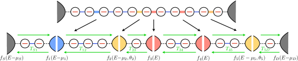
Figure 2: A tight-binding chain is connected to source and drain reservoirs and driven to non-equilibrium by different chemical potentials $\mu_{S/D}$ and temperatures $\theta_{S/D}$. Decoherence, energy redistribution and dissipation are introduced in the chain by replacing bonds with decoherence reservoirs according to the probabilities in Figure 1. In the blue shaded reservoir of $f_{1}(E-\mu_{1})$ the electrons dissipate energy to a heat bath of fixed temperature $\theta_{\mathrm{bath}}$. In the yellow shaded reservoirs of $f_{2}(E-\mu_{2},\theta_{2})$ and $f_{5}(E-\mu_{5},\theta_{5})$ the electrons redistribute their energy. In the red shaded reservoirs of $f_{3}(E)$ and $f_{4}(E)$ the electron energy is unchanged. Note that the arguments of the distribution functions $f_{i}$ are used to distinguish between the three different cases.

Decoherence regions are introduced by replacing with the probabilities given in Figure 1 the $N$ bonds of the chain by decoherence reservoirs, see Figure 2 (lower part). For energy conserving decoherence ($p_{r}=p_{d}=0)$, we have already used this approach successfully in our previous work [36, 38, 37, 40, 39]. As the phase coherence is lost completely in the decoherence regions, the chain is divided into smaller coherent subsystems. The phase coherent transport within the subsystems is characterized by transmission functions $T_{i,i+1}(E)$, which can be calculated by means of the non-equilibrium Green’s function (NEGF) method, as we did in our previous work. However, in this article we focus on the effects of decoherence, energy redistribution and dissipation and assume $T_{i,i+1}(E)=T(E)=1$ within all subsystems for all considered energies.

The subdivision into smaller coherent subsystems keeps the computational demand of our model moderate: The coherent transmission has to be calculated only between neighboring reservoirs. Moreover each of these calculations is less heavy (for $p>1/N$), as it involves one-electron Hilbert spaces of average dimension $1/p$ instead of $N$. The ensemble average can be truncated usually after a few hundred realizations. This makes our model in large systems with weak decoherence computationally more efficient than the original Pastawski model [30]. However, we would like to mention that other work has also been done to improve the performance of Pastawski’s model [25, 33].

The decoherence reservoirs are coupled by rate equations, which express conservation laws depending on the type of decoherence. In the following two subsections we discuss these rate equations for general $T$ and solve them analytically for $T=1$.

2.1 Rate equations for the distribution functions

The difference between the incoming and outgoing current of electrons with energy $E$ at a decoherence reservoir $i$ is given by

$$\mathcal{I}(E)\equiv T_{i-1,i}(E)\left(f_{i-1}{-}f_{i}\right)+T_{i+1,i}(E)\left(f_{i+1}{-}f_{i}\right).$$ (2)

If this decoherence reservoir is energy conserving, the equation

$$\mathcal{I}(E)=0$$ (3)

has to be fulfilled in steady state. In this case $f_{i}$ is a non-equilibrium distribution function $f_{i}(E)$, while the neighboring reservoirs $f_{i+1}$ and $f_{i-1}$ can be non-equilibrium functions or Fermi functions.

At an energy dissipating decoherence reservoir electrons loose energy to a heat bath (in the present case kept at zero temperature, $\theta_{\mathrm{bath}}=0$). Therefore only the charge integrated over all energies is conserved, i.e. Equation (2) is replaced by

$$\int\mathrm{d}E\,\mathcal{I}(E)=0$$ (4)

This equation determines the local chemical potential $\mu_{i}$ for the Fermi distribution $f_{i}=f_{i}(E-\mu_{i})$ with absolute temperature equal to $\theta_{\mathrm{bath}}=0$.

At a decoherence reservoir, where the electron energies are redistributed, Equation (4) must hold, too. As the energy remains in the electron system, furthermore the equation

$$\int\mathrm{d}E\,E\,\mathcal{I}(E)=0,$$ (5)

must be obeyed as well. The two Equations (4) and (5) then determine the local chemical potential $\mu_{i}$ and the local temperature $\theta_{i}$ of the Fermi function $f_{i}=f_{i}(E-\mu_{i},\theta_{i})$. Obviously, they depend on the distribution functions at the neighboring decoherence reservoirs.

2.2 Solution of the rate equations for $T(E)=1$

For transmission $T(E)=1$ the rate equations can be solved analytically by the Sommerfeld expansion. Let us consider a given decoherence configuration of $N_{D}$ decoherence reservoirs of which $N_{D}^{\mathrm{ex}}$ are energy exchanging (redistributing and dissipating). Let $N_{i}$ denote the number of energy conserving decoherence reservoirs between the $i$th and $(i+1)$th energy exchanging reservoir. For example, the decoherence configuration in Figure 2 consists of $N_{D}=5$ decoherence reservoirs of which $N_{D}^{\mathrm{ex}}=3$ are energy exchanging. The decoherence configuration contains only one line of two energy conserving reservoirs and hence $N_{2}=2.$ Solving Equation (2), the energy distribution function of the $q_{i}$th energy conserving reservoir after the $i$th energy exchanging reservoir is given by

$$f_{q_{i}}=\frac{N_{i}+1-q_{i}}{N_{i}+1}f_{i}+\frac{q_{i}}{N_{i}+1}f_{i+1},\quad q_{i}=1,2\dots N_{i},$$ (6)

where $f_{i}$ and $f_{i+1}$ are the Fermi distributions of the confining energy exchanging decoherence reservoirs (e.g. $f_{2}$ and $f_{5}$ in Figure 2). Hence, the energy distribution functions of the energy conserving decoherence reservoirs are (thermally broadened) double step functions. The positions of the steps are determined by the chemical potential of the confining energy exchanging reservoirs. The step height is given by the position $q_{i}$ in the line of energy conserving reservoirs.

Inserting Equation (6) in Equation (4) and using the Sommerfeld expansion for integrals of the Fermi function [41], we obtain for the chemical potential of the $i=1\dots N_{D}^{\mathrm{ex}}$ energy exchanging decoherence reservoirs

$$\mu_{i}=\mu_{S}-\frac{r_{i}}{N_{D}+1}(\mu_{S}-\mu_{D}).$$ (7)

where $r_{i}=\sum_{j=0}^{i-1}(N_{j}+1)$ gives the position of the $i$th energy exchanging reservoir in the line of all decoherence reservoirs. The chemical potential decreases linearly in the line of all decoherence reservoirs but this is not necessarily the case in real space, as the positions of the decoherence reservoirs are chosen randomly.

Let $M_{i}$ be the number of decoherence reservoirs between the $i$th and $(i+1)$th decoherence reservoir with fixed temperature (e.g. $M_{1}=4$ in Figure 2). Using again the Sommerfeld expansion as well as the previous results, we obtain for the temperatures of the subset of the $s_{i}$ decoherence reservoirs after the $i$th reservoir of fixed temperature (e.g. $s_{1}\in\{1,4\}$ in Figure 2)

$$\theta_{s_{i}}^{2}=\frac{3}{\pi^{2}}(\mu_{i}{-}\mu_{i+1})^{2}\frac{s_{i}}{M_{i}{+}1}\left(1{-}\frac{s_{i}}{M_{i}{+}1}\right)+\left(\theta_{i}^{2}{-}\theta_{i+1}^{2}\right)\frac{s_{i}}{M_{i}{+}1}+\theta_{i}^{2}.$$ (8)

Note that the second term in Equation (8) vanishes, if all dissipating reservoirs have the same temperature. The third term vanishes, if this temperature is set to zero.

Starting from the Boltzmann equation and assuming a linear decay of the chemical potential along the chain, it is discussed in Refs. [42, 43, 44, 45] that the temperature profile along the chain is determined by the differential equation

$$\frac{\pi^{2}}{6}\frac{d^{2}\theta^{2}}{dx^{2}}=-(\mu_{S}-\mu_{D})^{2}+\beta^{2}\left(\theta^{5}-\theta_{\mathrm{bath}}^{5}\right)$$ (9)

with the boundary conditions $\theta(0)=\theta(N+1)=\theta_{\mathrm{bath}}$. The first term in Equation (9) denotes the electron-electron scattering, whereas the second term controls via the parameter $\beta$ the strength of the electron-phonon scattering. In Section 3 we will compare solutions of Equation (9) with our model.

2.3 Ensemble averaged distribution functions

Using the analytical solution of the preceding section, we can calculate for a given decoherence configuration the energy distribution functions at those bonds, which have been replaced by decoherence reservoirs. Those bonds, which have not been replaced and hence are part of coherent subsystems, are described by a more complicated density matrix. However, we do not consider only a single fixed decoherence configuration but an ensemble of random realizations. In order to determine the ensemble averaged energy distribution function $\braket{f}$ for a given bond $x$ of the chain, we consider from the ensemble of decoherence configurations only those realization where the bond $x$ has been chosen as a decoherence bond. The ensemble averaged distribution function $\braket{f}$ is then given by the arithmetic average over this subset.

3 Properties of the model

We discuss the properties of the presented model by means of a tight-binding chain of $N+1=101$ sites (i.e. 100 bonds) with transmission $T(E)=1$. The chemical potentials of the source and drain reservoirs are used to define the energy scale and hence, set to $\mu_{S}=-\mu_{D}=1$. The temperature of the source and drain, as well as the temperature of the dissipating decoherence reservoirs is set to $\theta_{\mathrm{bath}}=0$. We consider ensembles of $2\cdot 10^{4}/p$ configurations.

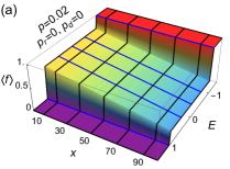
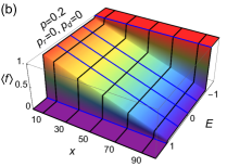
Figure 3: Ensemble averaged energy distribution function $\braket{f}$ of a tight-binding chain of length $N=100$. The decoherence probabilities have been fixed to $p=0.02$ (a) and $p=0.2$ (b) without energy redistribution $p_{r}=0$ nor energy dissipation $p_{d}=0$. Fixing the position $x$ in the chain, $\braket{f}$ shows two jumps at the chemical potential of source and drain $\mu_{S/D}=\pm 1$. At a fixed energy $\mu_{D}<E<\mu_{S}$, the distribution function is changing linearly and at the chain ends it jumps to $\braket{f}=1$ of the source and $\braket{f}=0$ of the drain.

Figure 3 shows the ensemble averaged energy distribution function $\braket{f}$ as a function of the electron energy $E$ and the position $x$ in the chain for two degrees of decoherence, $p=0.02$ (a) and $p=0.2$ (b). Neither energy redistribution ($p_{r}=0$) nor energy dissipation ($p_{d}=0$) are present. At a fixed position $0<x<101$, the distribution function $\braket{f}$ shows two steps at $E=\mu_{S/D}$ and is constant otherwise. A constant $0\leq\braket{f}\leq 1$ is observed in the energy range $\mu_{S}<E<\mu_{D}$, because the source is tending to occupy states in the chain while the drain is tending to empty these states. As the energy of the electrons is unchanged, the distribution function is constant in this energy range. Furthermore, for $E<\mu_{D}$ all states are occupied and for $E>\mu_{S}$ all states are unoccupied. At a fixed energy $\mu_{D}<E<\mu_{S}$, the distribution function decreases linearly along the chain. At the chain ends the distribution function shows two jumps to $\braket{f}=1$ at the source and $\braket{f}=0$ at the drain []. The height of these jumps decreases if the degree of decoherence increases. In the following, the effects of energy redistribution and dissipation are discussed focusing on the cases of strong decoherence ($p=0.2$) and weak decoherence ($p=0.02$).

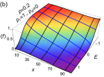
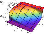
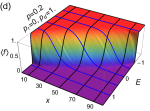
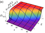
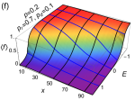
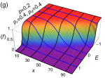
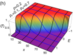
Figure 4: Energy distribution functions $\braket{f}$ under the effect of energy redistributing decoherence and energy dissipating decoherence. The degree of decoherence is fixed to $p=0.2$. In the first row, either energy redistribution (a,b) or energy dissipation are present (c,d). In (a,c) $p_{r}$ and $p_{d}$ are weak, while in (b,d) they are strong. In the second row, both types of scattering are mixed. We observe that energy redistribution transforms the double step function into a very smooth Fermi function, whereas energy dissipation causes a very steep Fermi function.

Figure 4 shows the energy distribution function for $p=0.2$ in presence of energy redistribution and dissipation. In the first row, either $p_{r}$ (a,b) or $p_{d}$ (c,d) are nonzero. For low $p_{r/d}$ (a,c) the jumps in the distribution functions are smoothed but still visible. In the range $\mu_{D}<E<\mu_{S}$ the distribution function is no longer constant but arched. In the case of high $p_{r/d}$ (b,d), the distribution function does not show a double step at the chemical potential of source and drain, anymore. Instead, it can be described by a Fermi function as will be discussed below. The distribution functions are quite different: For strong energy redistribution (b), the distribution function is much broader because the total energy of the electron system is unchanged. For strong energy dissipation (d), the distribution function is very steep, because the electrons dissipate their excess energy to a heat bath at zero temperature. Note that the redistribution of energy present in (a,b) allows for $\braket{f(E>\mu_{S})}>0$ and $\braket{f(E<\mu_{D})}<1$ corresponding to Auger processes. This is not possible if energy is dissipated to heat baths with $\theta_{\mathrm{bath}}=0$, see (c,d). In the second row of Figure 4, energy redistribution and dissipation are both present. Although the energy distribution functions are quite similar for some parameters, we can detect by means of their overall shape, if energy redistribution or energy dissipation are present and, if one of these processes dominates.

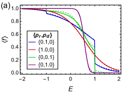
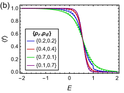
Figure 5: Ensemble averaged distribution function (solid curves) for $p=0.2$ and $x=20$. Fits with the model in Equation (10) (dashed curves) to the numerical data match excellently for all studied parameters.

The ensemble averaged energy distribution functions $\braket{f}$ give plenty of information about the electronic system of the tight-binding chain but they are difficult to analyze. Hence, our aim is to extract from $\braket{f}$ some few meaningful physical parameters, which characterize the system. This can be done by means of the model

$$\braket{f}_{\mathrm{fit}}(E,x)=a_{S}(x)f(E{-}\mu_{S})+a_{D}(x)f(E{-}\mu_{D})+a_{rd}(x)f(E{-}\mu(x),\theta(x)),$$ (10)

where $a_{S/D}\geq 0$ give the fraction (or relative densities) of electrons which follow the energy distribution function of source and drain, respectively. The parameter $a_{rd}\geq 0$ gives the fraction of thermalized electrons, which are described by a Fermi function with chemical potential $\mu$ and temperature $\theta$. The five parameters $\{a_{S/D/rd},\theta,\mu\}$ are determined from the numerical data in the following way. The two parameters $a_{S/D}$ are calculated from the height of the steps at $\mu_{S/D}$ in the distribution functions, because source and drain are at zero temperature. The remaining parameter $a_{rd}$ can be determined by using $f(E\to-\infty)=a_{S}+a_{D}+a_{rd}=1$. Hence, not five but only two parameters $\theta$ and $\mu$ are determined by a fit to the numerical data. Due to the symmetry of the boundary conditions and the homogeneity of the chain, the fit parameters fulfill the symmetry relations $a_{S}(x)=a_{D}(N-x)$, $a_{rd}(x)=a_{rd}(N-x)$, $\mu(x)=-\mu(N-x)$ and $\theta(x)=\theta(N-x)$. In general the model Equation (10) describes extremely well the numerical data. A typical example is shown in Figure 5.

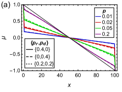
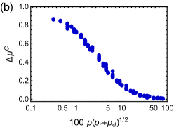
Figure 6: Left: Chemical potential in the chain. Within the chain the chemical potential decays linearly, while at the chain ends it jumps to $\mu_{S/D}=\pm 1$. These jumps can be attributed to the contact resistance of the chain. The thin black line represents a linear profile from the source to the drain. Right: Jumps of the chemical potential at the chain ends, calculated for various system parameters, as a function of $p\sqrt{p_{r}+p_{d}}$.

The chemical potential $\mu(x)$, determined by fitting the numerical data with Equation (10), is shown in Figure 6 (a). Inside the chain the chemical potential decays linearly, while at the chain ends it jumps abruptly to the fixed chemical potential $\mu_{S/D}=\pm 1$ of source and drain, respectively. As the chemical potential characterizes the potential energy of the electrons, its course can be interpreted as the voltage drop along the chain [46, 47]. Hence, we observe an Ohmic linear voltage profile inside the chain while the jumps at the chain ends $\Delta\mu^{C}$ can be attributed to the contact resistance of the chain [48, 49, 50]. The jumps are largest for low degree of decoherence $p$. They are symmetric because the source and drain reservoirs are identically coupled. If $p$ increases, $\Delta\mu^{C}$ diminishes and a linear voltage profile from the source to the drain is approached, see the thin black line. Such a linear voltage profile is one of the initial assumptions of the Boltzmann ansatz leading to Equation (9). By contrast, in our model the chemical potential profile is not an assumption but is calculated. Furthermore, we can model the entire regime from phase coherent to Ohmic transport. Figure 6 (b) shows that $\Delta\mu^{C}$ does not depend on $p,p_{r},p_{d}$ individually but only on the combination $p\sqrt{p_{r}+p_{d}}$. Other combinations of these three parameters would not lead to a collapse of the data on a single curve.

Note that only if $a_{rd}=1$ all electrons are described by a Fermi function. In general $\mu$ describes only the fraction of thermalized electrons, $a_{rd}<1$. This regime, in which a voltage drop in the Ohmic sense cannot be defined, is not covered by the Boltzmann ansatz in Refs. [42, 43, 44, 45] where all electrons are described by a Fermi function.

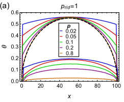
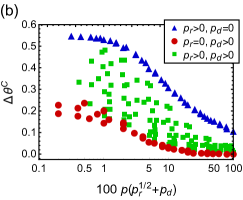
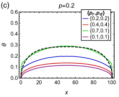
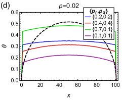
Figure 7: (a): Temperatures profiles $\theta(x)$ along the chain for various degree of decoherence $p$ in the case that either $p_{r}=1$ (top curves) or $p_{d}=1$ (bottom curves). When $p$ is increasing $\theta$ for $p_{r}=1$ approaches the black dashed curve, which is the solution of the Boltzmann model in Equation (9) for $\beta=0$. (b): Temperature jumps at the chain ends as a function of $p(\sqrt{p_{r}}+p_{d})$. (c,d): Temperatures for non-zero $p_{r}$ and $p_{d}$. The black dashed curve represents the temperatures from the Boltzmann ansatz with $\beta=22$ (c) and $\beta=2.2$ (d). In the case of strong decoherence ($p=0.2$) both models agree qualitatively, whereas they disagree in the case of weak decoherence ($p=0.02$), because the Boltzmann model does not describe coherent transport.

The temperature profile along the chain is shown in Figure 7 (a) for $p_{r}=1$ (top curves) and $p_{d}=1$ (bottom curves). When $p$ increases the temperature profile for $p_{r}=1$ approaches the black-dashed curve. This curve gives the solution of Equation (9) in the case $\beta=0$, which in turn is equivalent to the temperature profile in Equation (8) for $p=p_{r}=1$. Hence, in this limit case both models give identical results. When $p$ decreases, the temperature in the center of the chain stays constant but increases at the chain ends. For $p_{r}=1$ the Joule heat produced in the system can only be evacuated through the source and drain kept at zero temperature. For $p<1$ this causes abrupt jumps of the temperature at the chain ends, similar to those in the chemical potential. These temperature jumps $\Delta\theta^{C}$ can be attributed to the thermal contact resistance of the chain [51, 52, 53].

The temperature profile for $p_{d}=1$ approaches zero when $p$ is increased. This property is consistent with the fact that the electrons dissipate energy to heat baths at zero temperature. It is obtained also from Equation (9) in the limit $\beta\to\infty$. A finite temperature for $p<1$ arises in our model from statistical fluctuations. Physically this corresponds to a reduction of the cross-section for electron-phonon scattering, which prevents the electrons from dissipating all their excess energy to the heat baths.

The temperature jumps $\Delta\theta^{C}$ are shown in Figure 7 (b) as a function of $p(\sqrt{p_{r}}+p_{d})$ for various system parameters. In general, energy redistribution (blue triangles) leads to higher values of $\Delta\theta^{C}$ than energy dissipation (red dots). If either $p_{r}$ or $p_{d}$ are zero, the data points collapse onto single curves. If both are non-zero (green squares) the jumps $\Delta\theta^{C}$ and hence, the temperature along the chain depend on the individual values of $p_{r}$ and $p_{d}$. Note that the scaling properties of $\Delta\theta^{C}$ and the $\Delta\mu^{C}$ are different, compare with Figure 6 (b). If the data in Figure 7 (b) are plotted as a function of $p\sqrt{p_{r}+p_{d}}$, a data collapse on single curves (blue triangles and red dots) is not observed.

When either $p_{r}$ or $p_{d}$ are nonzero but less than 1, the temperature profiles show qualitatively the same behavior as in Figure 7 (a). However, in this case only the fraction $a_{rd}$ of the electrons is characterized by the temperature $\theta$. This reflects the fact that the system is in non-equilibrium and cannot be described by a thermodynamic temperature. Figure 7 (c,d) show the temperature profiles in the case that $p_{r}$ and $p_{d}$ have both non-zero values. In the case of strong decoherence ($p=0.2$) the calculated temperature profile agrees qualitatively with the temperature profile from the Boltzmann model Equation (9) using the fit parameter $\beta=22$, compare the solid green curve and the black dashed curve. For low decoherence ($p=0.02$) the black dashed curve, representing the solution of Equation (9) with $\beta=2.2$, disagrees with the temperature from our model, which is almost constant inside the chain with steep temperature drops at the chain ends. This disagreement is not surprising because the Boltzmann ansatz in Equation (9) does not describe coherent transport.

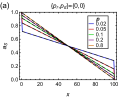
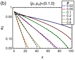
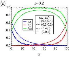
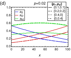
Figure 8: Fractions (or relative densities) of the electrons along the chain. $a_{S/D}$ represent the fraction of electrons which are unthermalized, while $a_{rd}$ gives the fraction of thermalized electrons. $a_{S}$ changes linearly if $p_{r}=p_{d}=0$, whereas it is dominated by an exponential decay if $p_{r}$ or $p_{d}$ are nonzero. The dashed black curve in (b) represent fits using Equation (11).

The fractions (or densities) of electrons, which follow a certain distribution function in Equation (10), are shown in Figure 8. The fraction of electrons following the source can be described by

$$a_{S}(x)=\frac{1+\tilde{a}}{2}\exp\left(-\frac{x}{\xi}\right)+\tilde{a}\frac{x}{N}\exp\left(-\frac{N}{\xi}\right)$$ (11)

with the two parameters $\tilde{a}$ and $\xi$. In the case $p_{r}+p_{d}=0$, the characteristic length $\xi\to\infty$ and $a_{S}$ decays linearly, see Figure 8 (a). This behavior can be understood by taking into account the symmetry relation $a_{S}(x)=a_{D}(N-x)$ and the particle conservation constraint. In the limit case of coherent transport ($p\sim 0$), we obtain $a_{S}=a_{D}=0.5$, because no scattering takes place in the chain and hence, its states are occupied equally by source and drain.

If $p_{r}$ or $p_{d}$ are nonzero, see for example Figure 8 (b), $a_{S}$ is dominated by the exponential decay close to the source while farther away linear corrections have to be taken into account. Figure 8 (c,d) show that the electron densities are functions of $p_{r}+p_{d}$. The fact that $a_{S/D/rd}$ and $\mu$ depend only on the sum $p_{r}+p_{d}$ while only $\theta$ depends on the individual values of $p_{r/d}$ makes the distribution functions for constant $p_{r}+p_{d}$ similar but not identical.

Due to the fact that we assumed for the transmission in the chain $T(E)=1$, the distribution functions show the following scaling law. Considering two different sets of parameters $\{N,p,p_{r},p_{d}\}$ and $\{N^{\prime},p^{\prime},p_{r}^{\prime},p_{d}^{\prime}\}$, the distribution functions of long chains ($N\gg 1$) are identical, if the parameters fulfill $Npp_{r/d}=N^{\prime}p^{\prime}p_{r/d}^{\prime}$. Note that this scaling law is restricted by the constraint $0\leq p,p_{r/d},p_{r}+p_{d}\leq 1$. The scaling law breaks down if $p\sim 0$, because effects of the coherent transport become important.

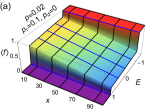
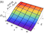
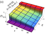
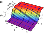
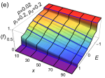
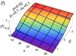
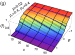
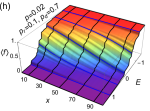
Figure 9: Energy distribution functions $\braket{f}$ under the effect of energy redistributing decoherence and energy dissipating decoherence. The parameters are the same as in Figure 4, apart from the fact that the degree of decoherence $p=0.02$.

Figure 9 shows the ensemble averaged energy distribution function in the case of weak decoherence $p=0.02$. The shape of the distribution function agrees qualitatively with the results for $p=0.2$ shown in Figure 4. However, if $p_{d}>0$ we observe, apart from the steps at $\mu_{S/D}=\pm 1$, several smaller steps. These steps can be seen even more clearly in Figure 10, where $\braket{f(x=20)}$ is shown. They cannot be reproduced by the model Equation (10), which apart from that fits very well to the numerical data. The small steps in $\braket{f}$ can be attributed to the steps in the zero-temperature Fermi function of the energy dissipating decoherence reservoirs. For low $p$, a decoherence configuration consists of only some few decoherence reservoirs (in average two for $p=0.02$ and $N=100$), which are either energy conserving, energy redistributing or dissipating. This restricts strongly the number of possible Fermi energies and causes jumps of considerable height in $\braket{f}$. This behavior becomes even more pronounced if $p_{d}\sim 1$, compare the solid green and purple curves in Figure 10 (a). If $p$ is not close to zero, the Fermi energy can adopt many different values and hence, the steps in the distribution function vanish []. This effect is smoothed out if a nonzero bath temperature is assumed. For the same reason this effect is not observed for energy redistributing decoherence, where the hot electrons relax to Fermi function of nonzero temperature. Jumps in the distribution functions are reported also in [54], where a chain with superconducting leads is modeled. In both cases the jumps are due to a characteristic interaction. While in this work jumps are due to a weakly distributed ($p$ low) but very effective ($p_{d}$ high) energy dissipating scattering, in [54] multiple Andreev reflections are present.

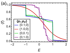
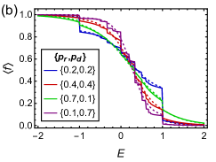
Figure 10: Energy distribution function at $x=20$. In comparison to Figure 5 several smaller steps are observed. The model in Equation (10) cannot reproduce these steps. Apart from this it matches the numerical data.

4 Application to carbon nanotube experiments

In this Section, we apply our model to the experiment in [7], where the energy distribution function at a fixed position of a carbon nanotube is obtained from non-equilibrium tunneling spectroscopy. A single-wall nanotube of length larger than $1\,\mathrm{\mu m}$ was studied at temperature $\theta_{\mathrm{bath}}=1.3\,\mathrm{K}$. The energy of the conduction electrons was controlled by a gate voltage. The solid black curves in Figure 11 are the experimental data for a bias voltage of $U=1\,\mathrm{mV}$ and the different gate voltages (from left to right) $8.660\,\mathrm{V},8.285\,\mathrm{V},8.070\,\mathrm{V}$, taken from Figure 4 (a-c) of [7]. Note that in order to show the three curves more clearly in a single figure, we have shifted them by arbitrary energy constants. At the large and the small gate voltage one observes (thermally broadened) double step energy distribution functions consistent with the difference of $1\,\mathrm{meV}$ between the source and drain chemical potentials, which indicate ballistic transport in the carbon nanotube. For the intermediate gate voltage, however, no remainder of the double step can be seen. As an explanation it is suggested in [7] that defect scattering is switched on by the intermediate gate voltage, while it is largely suppressed by the other two values.

The experimental data agree well with results from our model, if the parameters are chosen appropriately, see the dashed curves in Figure 11. Instead of a microscopic tight-binding model, in which all Carbon atoms of the nanotube are taken into account [55], we use a coarse grained description: The nanotube of total length $L$ is divided into $Np=100$ segments of length $\ell_{\phi}$ each. Therefore we represent each cell by a decoherence region of a one dimensional chain. A fraction $p_{d}$ of these regions is energy dissipating, a fraction $p_{r}$ is energy redistributing. These are the only fit parameters, because the bias voltage and the temperature are set to the same values as in the experiment. The lengths $\ell_{\mathrm{red/dis}}=1/(Npp_{r/d})$ measured in units of the nanotube length $L$ are given in the inset of Figure 11. As $\ell_{\mathrm{red}}\geq\ell_{\mathrm{dis}}$, we conclude that in this experimental setup it is more likely that an electron of the Carbon nanotube exchanges energy with a heatbath than redistributing it within the electron system. The heatbath could for example be the superconducting probe. The fact that both scattering lengths are of the order of the nanotube length or larger shows that scattering is really weak in this experiment.

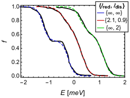
Figure 11: Application of our model to the carbon-nanotube experiments in [7]. The scattering lengths, given in the inset in units of the nanotube length, are determined by fitting our model to the data. Note that all curves have been shifted by some constant energy in order to show several measurements in a single figure.

5 Conclusions

We have introduced a statistical model for the effects of decoherence, energy redistribution and energy dissipation on the distribution function along a one-dimensional system driven out of equilibrium by a source and a drain with different chemical potentials. Note that our model gives a uniform Fermi-Dirac distribution throughout the system, if source and drain and the heat baths coupled to the chain are in equilibrium. The essential idea of the model is to concentrate decoherence exclusively in local regions, distributed stochastically in the system with probability $p$. In these decoherence regions phase information about the electron state is lost entirely, while its energy may be exchanged with a heat-bath (e.g. lattice vibrations) with probability $p_{d}$, or be redistributed among the electrons with probability $p_{r}$, or otherwise remain unchanged. One-dimensional quantum systems are divided by the decoherence regions into smaller coherent subsystems, which makes our model computationally efficient. The probabilities, with which the decoherence regions occur, are then inversely proportional to the scattering lengths of the system. The energy distribution functions of the decoherence regions are coupled by rate equations, which have been solved analytically for the case, that the coherent electron transmission between decoherence regions can be described by $T(E)=1$. By ensemble averaging over the spatial decoherence configurations, energy distribution functions are calculated everywhere in the quantum system, see Figure 4 and 9. Their shape depends on the distance from source and drain and on the relative strength of the three types of decoherence (energy dissipating, redistributing, or conserving). These non-equilibrium distribution functions turned out to be a weighted sum of three Fermi functions, two of which belong to source or drain, respectively. Their contributions decay exponentially with distance from source and drain, if energy dissipation or redistribution occur. The third Fermi function belongs to the fraction of thermalized electrons. The temperature and chemical potential depend on the distance from source and drain, and on the scattering lengths. Our model also describes the electrical and thermal contact resistances at the electrodes, which lead to discontinuities of the chemical potential and the temperature for weak decoherence. That the model provides a useful tool for evaluating experiments, has been shown for data obtained by non-equilibrium tunneling spectroscopy for a Carbon nanotube [7]. The excellent agreement of our model with the experimental data has allowed to determine the scattering lengths of the nanotube. In the future, we will apply our model to cases, where $T(E)\neq 0$, for example to DNA chains. We also plan to extend our model to pure dephasing by the possibility of adjusting independently the degree of phase and momentum randomization [36]. The extension of our model to time dependent problems is also considered [56, 57].

References

References

- [1] Shulaker M M, Hills G, Patil N, Wei H, Chen H Y, Wong H S P and Mitra S 2013 Nature 501 526–530 URL http://dx.doi.org/10.1038/nature12502
- [2] Brady G J, Way A J, Safron N S, Evensen H T, Gopalan P and Arnold M S 2016 Science Advances 2 e16012401 URL http://dx.doi.org/10.1126/sciadv.1601240
- [3] Privman V, Vagner I and Kventsel G 1998 Phys. Lett. A 239 141–146 URL http://www.sciencedirect.com/science/article/pii/S0375960197009742
- [4] Žutić I, Fabian J and Das Sarma S 2004 Rev. Mod. Phys. 76 323–410 URL http://link.aps.org/doi/10.1103/RevModPhys.76.323
- [5] Pothier H, Guéron S, Birge N O, Esteve D and Devoret M H 1997 Phys. Rev. Lett. 79 3490–3493 URL http://link.aps.org/doi/10.1103/PhysRevLett.79.3490
- [6] Pothier H, Guéron S, Birge N O, Esteve D and Devoret M H 1997 Zeitschrift für Physik B 103 313–318 URL http://dx.doi.org/10.1007/s002570050379
- [7] Chen Y F, Dirks T, Al-Zoubi G, Birge N and Mason N 2009 Phys. Rev. Lett. 102 036804 URL http://link.aps.org/doi/10.1103/PhysRevLett.102.036804
- [8] Bronn N and Mason N 2013 Phys. Rev. B 88 161409 URL http://link.aps.org/doi/10.1103/PhysRevB.88.161409
- [9] le Sueur H, Altimiras C, Gennser U, Cavanna A, Mailly D and Pierre F 2010 Phys. Rev. Lett. 105 056803 URL http://link.aps.org/doi/10.1103/PhysRevLett.105.056803
- [10] Altimiras C, le Sueur H, Gennser U, Cavanna A, Mailly D and Pierre F 2010 Nat. Phys. 6 34–39 URL http://dx.doi.org/10.1038/nphys1429
- [11] Altimiras C, le Sueur H, Gennser U, Cavanna A, Mailly D and Pierre F 2010 Phys. Rev. Lett. 105 226804 URL http://link.aps.org/doi/10.1103/PhysRevLett.105.226804
- [12] Voutilainen J, Fay A, Häkkinen P, Viljas J K, Heikkilä T T and Hakonen P J 2011 Phys. Rev. B 84 045419 URL http://link.aps.org/doi/10.1103/PhysRevB.84.045419
- [13] Gutman D B, Gefen Y and Mirlin A D 2009 Phys. Rev. B 80 045106 URL http://link.aps.org/doi/10.1103/PhysRevB.80.045106
- [14] Levkivskyi I and Sukhorukov E 2012 Phys. Rev. B 85 075309 URL http://link.aps.org/doi/10.1103/PhysRevB.85.075309
- [15] Degiovanni P, Grenier C, Fève G, Altimiras C, le Sueur H and Pierre F 2010 Phys. Rev. B 81 121302 URL http://link.aps.org/doi/10.1103/PhysRevB.81.121302
- [16] Kovrizhin D L and Chalker J T 2012 Phys. Rev. Lett. 109 106403 URL http://link.aps.org/doi/10.1103/PhysRevLett.109.106403
- [17] Lunde A M, Nigg S E and Büttiker M 2010 Phys. Rev. B 81 041311 URL http://link.aps.org/doi/10.1103/PhysRevB.81.041311
- [18] Lunde A M and Nigg S E 2016 Phys. Rev. B 94 045409 URL http://link.aps.org/doi/10.1103/PhysRevB.94.045409
- [19] Dolcini F, Iotti R and Rossi F 2013 Phys. Rev. B 88 115421 URL http://link.aps.org/doi/10.1103/PhysRevB.88.115421
- [20] Karzig T, Glazman L I and von Oppen F 2010 Phys. Rev. Lett. 105 226407 URL http://link.aps.org/doi/10.1103/PhysRevLett.105.226407
- [21] Pepe M, Taj D, Iotti R C and Rossi F 2012 physica status solidi (b) 249 2125–2136 URL http://dx.doi.org/10.1002/pssb.201147541
- [22] Dolcini F, Iotti R C and Rossi F 2014 Microscopic Modeling of Solid-State Quantum Devices (Springer) pp 1–21 URL http://dx.doi.org/10.1007/978-94-007-6178-0_100945-1
- [23] Büttiker M 1986 Phys. Rev. B 33 3020–3026 URL http://dx.doi.org/10.1103/PhysRevB.33.3020
- [24] Datta S 1989 Physical Review B 40 5830–5833 URL http://link.aps.org/doi/10.1103/physrevb.40.5830
- [25] Pastawski H M 1991 Phys. Rev. B 44(12) 6329–6339 URL http://link.aps.org/doi/10.1103/PhysRevB.44.6329
- [26] Datta S and Lake R K 1991 Phys. Rev. B 44(12) 6538–6541 URL http://link.aps.org/doi/10.1103/PhysRevB.44.6538
- [27] Hershfield S 1991 Phys. Rev. B 43 11586–11594 URL http://link.aps.org/doi/10.1103/PhysRevB.43.11586
- [28] Datta S 1992 Phys. Rev. B 46(15) 9493–9500 URL http://link.aps.org/doi/10.1103/PhysRevB.46.9493
- [29] Pastawski H M and Medina E 2001 Revista Mexicana de Física 47 Suplemento 1 1–23 URL https://arxiv.org/abs/cond-mat/0103219
- [30] D’Amato J L and Pastawski H M 1990 Phys. Rev. B 41 7411–7420 URL http://dx.doi.org/10.1103/PhysRevB.41.7411
- [31] Cattena C J, Bustos-Marún R A and Pastawski H M 2010 Phys. Rev. B 82 144201 URL http://dx.doi.org/10.1103/PhysRevB.82.144201
- [32] Nozaki D, Gomes da Rocha C, Pastawski H M and Cuniberti G 2012 Phys. Rev. B 85 155327 URL http://link.aps.org/doi/10.1103/PhysRevB.85.155327
- [33] Nozaki D, Bustos-Marún R, Cattena J C, Cuniberti G and Pastawski M H 2016 Eur. Phys. J. B 89 1–7 URL http://dx.doi.org/10.1140/epjb/e2016-70013-y
- [34] Roy D and Dhar A 2007 Phys. Rev. B 75 195110 URL http://link.aps.org/abstract/PRB/v75/e195110
- [35] Zilly M, Ujsághy O and Wolf D E 2009 Eur. Phys. J. B 68 237–246 URL http://dx.doi.org/10.1140/epjb/e2009-00101-0
- [36] Stegmann T, Zilly M, Ujsághy O and Wolf D E 2012 Eur. Phys. J. B 85 264 URL http://dx.doi.org/10.1140/epjb/e2012-30348-y
- [37] Zilly M, Ujsághy O and Wolf D E 2010 Phys. Rev. B 82 125125 URL http://dx.doi.org/10.1103/PhysRevB.82.125125
- [38] Zilly M, Ujsághy O, Woelki M and Wolf D E 2012 Phys. Rev. B 85 075110 URL http://link.aps.org/doi/10.1103/PhysRevB.85.075110
- [39] Stegmann T, Ujsághy O and Wolf D E 2014 Eur. Phys. J. B 87 30 URL http://dx.doi.org/10.1140/epjb/e2014-40997-3
- [40] Stegmann T, Wolf D E and Lorke A 2013 New J. Phys. 15 113047 URL http://stacks.iop.org/1367-2630/15/i=11/a=113047
- [41] Sólyom J 2009 Fundamentals of the Physics of Solids vol 2 (Springer)
- [42] Nagaev K E 1995 Phys. Rev. B 52 4740–4743 URL http://link.aps.org/doi/10.1103/PhysRevB.52.4740
- [43] Kozub V I and Rudin A M 1995 Phys. Rev. B 52 7853–7856 URL http://link.aps.org/doi/10.1103/PhysRevB.52.7853
- [44] Naveh Y, Averin D V and Likharev K K 1998 Phys. Rev. B 58 15371–15374 URL http://link.aps.org/doi/10.1103/PhysRevB.58.15371
- [45] Huard B, Pothier H, Esteve D and Nagaev K E 2007 Phys. Rev. B 76 165426 URL http://link.aps.org/doi/10.1103/PhysRevB.76.165426
- [46] Datta S 1997 Electronic Transport in Mesoscopic Systems (Cambridge University Press)
- [47] McLennan M J, Lee Y and Datta S 1991 Phys. Rev. B 43 13846–13884 URL http://dx.doi.org/10.1103/PhysRevB.43.13846
- [48] Lan C, Srisungsitthisunti P, Amama P B, Fisher T S, Xu X and Reifenberger R G 2008 Nanotechnology 19 125703 URL http://stacks.iop.org/0957-4484/19/i=12/a=125703
- [49] Ho Choi S, Kim B and Frisbie C D 2008 Science 320 1482–1486 URL http://science.sciencemag.org/content/320/5882/1482
- [50] Liu H, Wang N, Zhao J, Guo Y, Yin X, Boey F Y C and Zhang H 2008 ChemPhysChem 9 1416–1424 URL http://dx.doi.org/10.1002/cphc.200800032
- [51] Fujii M, Zhang X, Xie H, Ago H, Takahashi K, Ikuta T, Abe H and Shimizu T 2005 Phys. Rev. Lett. 95 065502 URL https://link.aps.org/doi/10.1103/PhysRevLett.95.065502
- [52] Pop E, Mann D, Wang Q, Goodson K and Dai H 2006 Nano Lett. 6 96–100 URL http://dx.doi.org/10.1021/nl052145f
- [53] Pop E 2008 Nanotechnology 19 295202 URL http://stacks.iop.org/0957-4484/19/i=29/a=295202
- [54] Apostolov S S and Levchenko A 2014 Phys. Rev. B 89 201303 URL http://link.aps.org/doi/10.1103/PhysRevB.89.201303
- [55] Reich S, Thomsen C and Maultzsch J 2004 Carbon Nanotubes (Wiley-VCH)
- [56] Rethfeld B, Kaiser A, Vicanek M and Simon G 2002 Phys. Rev. B 65 214303 URL http://link.aps.org/doi/10.1103/PhysRevB.65.214303
- [57] Medvedev N and Rethfeld B 2010 Journal of Applied Physics 108 103112 URL http://scitation.aip.org/content/aip/journal/jap/108/10/10.1063/1.3511455