The New Horizons and Hubble Space Telescope Search For Rings, Dust, and Debris in the Pluto-Charon System

Abstract

We conducted an extensive search for dust or debris rings in the Pluto-Charon system before, during, and after the New Horizons encounter in July 2015. Methodologies included attempting to detect features by back-scattered light during the approach to Pluto (phase angle $\alpha\sim 15^{\circ}$), in situ detection of impacting particles, a search for stellar occultations near the time of closest approach, and by forward-scattered light imaging during departure ($\alpha\sim 165^{\circ}$). An extensive search using the Hubble Space Telescope (HST) prior to the encounter also contributed to the final ring limits. No rings, debris, or dust features were observed, but our new detection limits provide a substantially improved picture of the environment throughout the Pluto-Charon system. Searches for rings in back-scattered light were covered the range 35,000–250,000 km from the system barycenter, a zone that starts interior to the orbit of Styx, the innermost minor satellite, and extends out to four times the orbital radius of Hydra, the outermost known satellite. We obtained our firmest limits using data from the New Horizons LORRI camera in the inner half of this region. Our limits on the normal $I/F$ of an unseen ring depends on the radial scale of the rings: $2\times 10^{-8}$ ($3\sigma$) for 1500 km wide rings, $1\times 10^{-8}$ for 6000 km rings, and $7\times 10^{-9}$ for 12,000 km rings. Beyond $\sim 100,000$ km from Pluto, HST observations limit normal $I/F$ to $\sim 8\times 10^{-8}$. Searches for dust features from forward-scattered light extended from the surface of Pluto to the Pluto-Charon Hill sphere ($r_{\rm Hill}=6.4\times 10^{6}$ km). No evidence for rings or dust clouds was detected to normal $I/F$ limits of $\sim 8.9\times 10^{-7}$ on $\sim 10^{4}$ km scales. Four stellar occulation observations also probed the space interior to Hydra, but again no dust or debris was detected. The Student Dust Counter detected one particle impact $3.6\times 10^{6}$ km from Pluto, but this is consistent with the interplanetary space environment established during the cruise of New Horizons. Elsewhere in the solar system, small moons commonly share their orbits with faint dust rings. Our results support recent dynamical studies suggesting that small grains are quickly lost from the Pluto-Charon system due to solar radiation pressure, whereas larger particles are orbitally unstable due to ongoing perturbations by the known moons.

1 Searching For Rings and Dust Around Pluto

1.1 Could Pluto Have Rings?

It is likely that Pluto had rings at various times in its history, although their existence may have been fleeting. The standard model for the formation of both Charon and the four minor satellites of Pluto is that they were created in a collision between Pluto and another large KBO (McKinnon, 1989; Canup, 2005; Stern et al., 2006), which would have created an extensive debris disk. Dynamical interactions would have quickly cleared most of the larger debris, and solar radiation pressure sweeps away much of the fine dust (Pires dos Santos et al., 2013); however, it is plausible that remnants of this initial event could have persisted at large radii into the present (Kenyon & Bromley, 2014). The recent discovery of rings around the Centaur-object (10199) Chariklo (Braga-Ribas et al., 2014), and possibly Chiron (2060) (Ruprecht et al., 2015; Ortiz et al., 2015), vividly demonstrates that small solar system bodies may indeed possess rings in their own right (also see the discussion in Sicardy et al. 2016).

Apart from “fossil” rings left over from the initial creation of the satellite system, we might expect to find diffuse dust rings arising from ongoing impact erosion of the minor satellites. Durda & Stern (2000) argued that the frequency of collisions within the Kuiper Belt is high enough to cause significant erosion of all small KBOs over the age of the solar system. In the specific context of Pluto, Stern et al. (2006), Steffl & Stern (2007), Stern (2009), and Poppe & Horányi (2011) predicted that impact gardening of the minor satellites Hydra and Nix (and by implication Kerberos and Styx, which were discovered later) could inject fine debris or dust into the environment around Pluto and Charon, leading to transitory or long-lived rings. (Escape velocities are too high for this mechanism to generate rings directly from Pluto or Charon.)

On theoretical grounds, Stern et al. (2006) estimated that a ring generated from steady-state erosion of Hydra and Nix would have optical depth $\tau=5\times 10^{-6}.$ Poppe & Horányi (2011) argued for a shorter particle lifetime, yielding $\tau=10^{-7}.$ Given the dynamic complexity of Pluto and Charon plus the four minor satellites, a key theoretical problem is identifying orbits that can host stable rings. Poppe & Horányi (2011) and Pires dos Santos et al. (2013) showed, for example, that long-lived rings could exist between the orbits of Nix and Hydra, as well as at co-orbital locations in the orbits of the four minor satellites. However, the subsequent discovery of Kerberos orbiting between these two moons partially invalidated their conclusions (Porter & Stern, 2015).

On the other hand, Pires dos Santos et al. (2013) argued that solar radiation pressure is sufficient, even at the distance of Pluto, to clear small particles from the system, given Pluto’s overall shallow gravity well. They predicted that the optical depth of any long-lived dust ring would be no more than $4\times 10^{-11},$ well below any feasible detection limits. This result holds despite the substantial rates of impact gardening estimated by Durda & Stern (2000) (a significantly lower rate may be implied by the crater counts measured by Singer et al. 2017). Furthermore, simulations by Youdin et al. (2012) and Showalter & Hamilton (2015) show the system to be chaotic, raising questions about the long-term stability of the small moons themeselves, irrespective of any embedded rings. Interior to the orbit of Charon, long-lived rings are unlikely to exist due to the drag induced by Pluto’s extended atmosphere (Porter & Grundy, 2015).

Because this debate has been inconclusive, it remained an open question whether Pluto might have faint rings above the sensitivity threshold of the New Horizons (NH) cameras. Beyond the scientific interest in such rings, their possible existence also raised concerns about a potential hazard to the spacecraft during its passage through the system.

1.2 Previous Searches for Plutonian Rings

A few attempts were made to detect rings in advance of the NH encounter. Steffl & Stern (2007) used high-resolution images of Pluto and Charon taken with the ACS/HRC instrument on board the Hubble Space Telescope (HST) to derive upper limits for the visibility of any rings in back-scattered, visual-band sunlight. Their detection limits were controlled by the scattered-light background and thus varied with projected distance from Pluto. At the orbit of Hydra, they limited the rings’ normal $I/F$ to $\sim 2.5\times 10^{-7}$. That limit approximately doubles at the inner limit of orbital stability, which is $\sim 42$,000 km.

Like Steffl & Stern (2007), we measure intensity $I$ by the dimensionless ratio $I/F$, where $\pi F$ is the incoming solar optical flux density at Pluto. With this definition, $I/F$ would equal unity for a perfectly diffusing “Lambert” surface when illuminated and viewed normal to the sunlight. For a body with geometric albedo $A$ viewed at phase angle $\alpha$, its surface reflectivity would be $I/F=A~{}P(\alpha)/P(0)$, where $P$ is the phase function.

Above, we quote values of “normal” $I/F\equiv\mu I/F$, which is a more useful quantity for describing optically thin rings. Here the observed $I/F$ is scaled by a factor $\mu={\rm cos}(e)$, where $e$ is the emission angle measured from the ring plane normal. The $\mu$ factor compensates for the apparent brightening of an optically thin ring when viewed closer to the ring plane, so normal $I/F$ describes the reflectivity that would be detected if $e=0$. Normal $I/F$ and optical depth $\tau$ are related via

$$\mu I/F=\tau A\times P(\alpha)/P(0).$$ (1)

For Steffl & Stern (2007), $A$ was extremely uncertain, plausibly ranging from 0.04 (for bodies resembling dark KBOs) to $\sim 0.38$, which is the geometric albedo of Charon. Today, we know that any ring dust is most likely to have albedos comparable to that of the nearby moons, for which $A=0.5$–0.9 (Weaver et al., 2016), higher than previously suspected. Nevertheless, because $I/F$ is the measured quantity in image analysis, we discuss most of our findings below in terms of normal $I/F$. We revisit the optical depth values in the final discussion and summary section.

Other techniques have also been applied to searches for rings of Pluto. Boissel et al. (2014) and Throop et al. (2015) separately used stellar occultations to search for rings. Occultations could potentially detect compact or narrow rings with widths well below the HST resolution limit. Unlike image measurements, occultations obtain $\tau$ directly; however, these experiments did not provide better limits for diffuse rings. Lastly, Marton et al. (2015) used far-IR images ($70~{}\mu{\rm m}$) from the Herschel Telescope to look directly for thermal emission from dust around Pluto and Charon, but again found limits broadly compatible with the HST results of Steffl & Stern (2007).

1.3 Overview

The initial summary of science results from the NH encounter noted that no dust features or rings with normal $I/F>10^{-7}$ were detected based on a preliminary analysis of the imaging searches conducted by the spacecraft during its approach (Stern et al., 2015). We have three goals for this dedicated ring-search paper that go beyond this initial result. The first is to summarize the results of a preliminary ring search performed using HST during 2011 and 2012. The second is to refine the limits derived from the initial analysis of NH data, as well as to present new limits based on data sets that had not yet been downlinked when Stern et al. (2015) was published. These include most of the deepest imaging obtained by the NH cameras. The third is to describe the NH search observations and associated analysis methodologies.

2 The HST Ring Search

In 2011, coauthors Showalter and Hamilton used HST to search for the putative rings of Pluto (HST-GO-12346). The prior search by Steffl & Stern (2007) was limited by the extensive glare surrounding Pluto and Charon. Showalter and Hamilton employed a “trick” to model and subtract this glare, potentially revealing rings $\sim 30$ times fainter than the previous upper limit. Their approach was to image the Pluto system during two HST visits that differed by a $90^{\circ}$ rotation of the camera. The visits were also timed to place Charon at roughly the same position relative to Pluto on the CCD (Fig. 1). The expectation was that that the glare patterns around Pluto and Charon, which are instrumental in origin, would be nearly identical in the two visits, but the rings (which are ellipses as projected onto the sky) would be rotated. By aligning and subtracting the images, most of the planetary glare would cancel out, leaving behind the signature of a ring as pair of crossed, positive and negative ellipses.

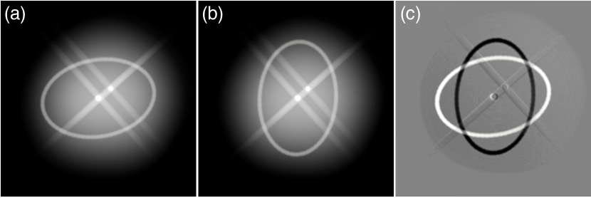
Figure 1: The HST imaging strategy employed to search for rings in 2011 and 2012. Panels (a) and (b) are cartoons of Pluto and Charon surrounded by a glare pattern plus a hypothetical ring. The camera has been rotated $90^{\circ}$ between the two exposures, so the glare pattern is similar but the rings have rotated. Panel (c) shows the difference between these two images. The glare pattern is nearly canceled out, but positive and negative images of the ring remain.

HST is constrained to keep its solar panels oriented toward the sun, so rotations $>10^{\circ}$ are not normally permitted. The exception is during a brief period around Pluto’s opposition, when the spacecraft can be oriented freely. Table 1 describes the visits and images obtained near the 2011 opposition. The “rotate-and-subtract” technique worked as planned (see below), although the processed images did not reveal any rings. However, because Showalter and Hamilton had obtained longer exposures of the Pluto system than anyone had previously attempted, these images revealed tiny Kerberos, Pluto’s fourth known moon (Showalter et al., 2011), which is $\sim 10$% as bright as Nix and Hydra.

Table 1: Ring Search Sequences with HST

Program	Visit	Date	Orbits	Filter	$T_{\rm exp}$	$N$	First filename	Orientation
GO-12346	21	2011-06-28	2	F606W	479	10	ibo821kvq_flt.fits	Horizontal
GO-12346	22	2011-07-03	2	F606W	479	10	ibo822taq_flt.fits	Vertical
GO-12801	31	2012-06-27	3	F350LP	174	35	ibxa31rmq_flt.fits	Horizontal
GO-12801	32	2012-07-09	3	F350LP	174	35	ibxa32cuq_flt.fits	Vertical
GO-12801	41	2012-06-29	3	F350LP	174	35	ibxa41bwq_flt.fits	Horizontal
GO-12801	43	2012-06-11	3	F350LP	174	35	ibxa43ebq_flt.fits	Vertical
GO-12801	61	2012-06-26	3	F350LP	174	35	ibxa61ifq_flt.fits	Horizontal
GO-12801	62	2012-07-07	3	F350LP	174	35	ibxa62o8q_flt.fits	Vertical

Note. — $T_{\rm exp}$ is the exposure time in seconds; $N$ is the number of images taken using this exposure time; Orientation indicates the approximate direction of the long axis of the ellipse representing a circular ring projected on the sky.

Following the Kerberos discovery, Weaver et al. (GO-12801) led a far more extensive HST observing program during Pluto’s 2012 opposition. The goal was to perform comprehensive search for rings and small moons. In addition to the scientific interest, these observations supported the programmatic goal of assessing possible hazards to the NH spacecraft during the upcoming Pluto flyby. This program revealed Styx, Pluto’s fifth moon (Showalter et al., 2012). Weaver et al. repeated the rotation “trick” of the previous year (Fig. 1), but with more integration time and a wider filter (Table 1). Here we derive the most sensitive Earth-based limits from a combined analysis of all these images.

2.1 Analysis Procedures

Figure 2a shows a typical image from Visit 31 in GO-12801. Because Pluto is located near the galactic center, numerous background stars are visible. Although visits span up to 4 hours, Pluto’s moons move only slightly in this time frame. HST time is measured in units of orbits of HST around the Earth, where each 95-minute orbit provides about 45 of Pluto viewing. Small dither steps in the middle of each HST orbit, and also between orbits, helped to mitigate the effects of hot pixels. Pluto and Charon saturated during these long exposures, but additional, short exposures of a few seconds show them clearly and without saturation. Within each orbit, we navigated the images using the unsaturated images of Pluto and Charon, plus Nix and Hydra from the longer exposures. From this information, we derived the pixel coordinates of the system barycenter within each image.

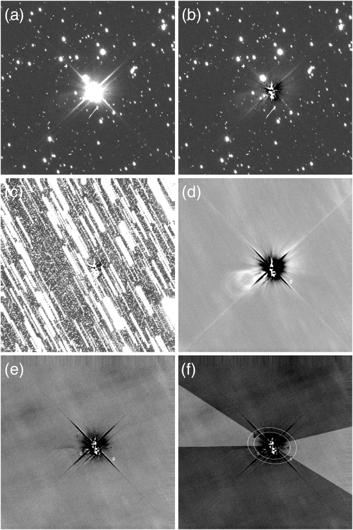
Figure 2: Steps in the processing of HST images. (a) The first image from Visit 31; see Table 1. (b) The same image after subtraction of PSF models for Pluto and Charon. (c) Our procedure to stack the images and sort the pixels at any location by intensity brings all the stars (and cosmic rays) to the front. (d) Stripping away the top layers and coadding the remainder produces a very clean image. This image has been enhanced by a factor of four relative to the image in the previous panel. (e) Subtracting pairs of perpendicular images would potentially reveal crossed positive and negative ellipses, but do not. (f) We derive radial profiles of the possible rings from wedges of the image defined to eliminate diffraction spikes, known moons, and other residual flaws. Darkened regions indicate pixels that are excluded. The orbits of Nix and Hydra are shown for reference.

After the navigation, we subtracted out the known bodies from the images. We used the program “Tiny Tim” (Krist et al., 2011) to model the point-spread function (PSF) for the images. We then applied a fitting procedure to locate and scale the PSF for each body. For Pluto and Charon, we also applied a small blur to account for the fact that these bodies are partially resolved by the instrument. We masked out the pixels where Pluto and Charon saturated, using only the unsaturated pixels for this modeling. The models produced by Tiny Tim are imperfect, but subtracting them suppresses much of the PSF, including most of the long diffraction spikes that extend diagonally outward from Pluto and Charon (Fig.2b).

At this stage, the bodies of the Pluto system have been suppressed, but background stars remain. A simple coadd of these images would be corrupted by the numerous stars. However, the stars are clearly identifiable by their motion between consecutive images. We devised a modified “coadd” procedure that is much more successful at suppressing the stars. We began by aligning all the images from each visit on the system barycenter and then stacking them into cubes. Within these cubes, we then sorted the pixels of each “column” from minimum to maximum, where the column is all pixels at the same pixel offset from the system barycenter in the image layers of the cube. This caused the background stars, as well as cosmic rays, to “rise to the top” (Fig. 2c). The final step was to eliminate the top layers and coadd the remainder (Fig. 2d)

In this processing, the key question was how many of the top layers to remove. Eliminating a fixed number of layers had the disadvantage that, in order to be sure all the stars were removed, many perfectly valid pixels were also excluded from the analysis. Our more refined procedure took advantage of the fact that, upon examining the trend in brightness going upward through each column of the stack, it was easy to identify the point at which a star first appeared (Fig. 3). Working upward through the pixels in each column, we defined the cutoff point as the first layer at which the value changed by more than $3\sigma$ relative to the calculated mean and standard deviation of the pixels below. Examples of the cutoff point are indicated in (Fig. 3); the result of this procedure for Visit 31 is shown in Fig. 2d.

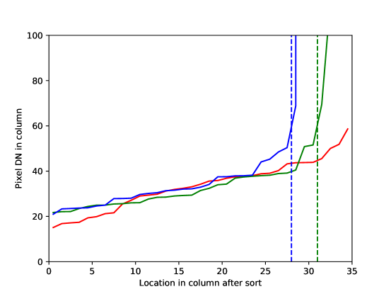
Figure 3: We plot DN vs. layer number in a selection of colums from the stack of 25 deep exposures taken during Visit 31. Near the right, large jumps upward correspond to background stars. Vertical dashed lines indicate the cutoff point; layers of the stack above this line are excluded from the coadding used to produce Fig. 2d. The red curve is well-behaved throughout, indicating that no stars were present at this location so all 35 layers could be coadded.

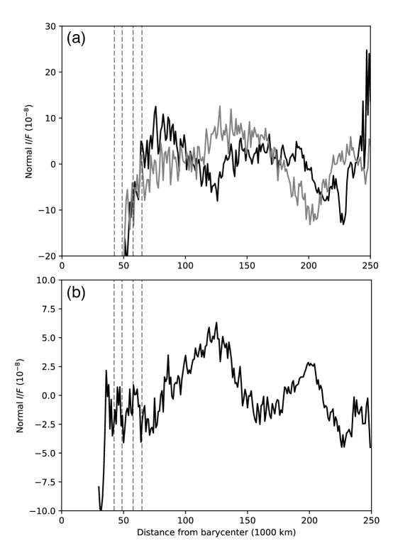
Figure 4: (a) Ring profiles derived from Visit 31 (cf. Fig. 2f). Linear trends, which are caused by subtle variations in the background glare pattern, have been removed. If rings are present, we would expect these profiles to show an increase at the same projected radius in each profile. Instead, the variations we see are uncorrelated and presumably caused by background gradients and residual stars. Vertical dashed lines indicate the orbits of the four small moons. (b) Coadding all the finest profiles produces our best Earth-based opportunity to detect Plutonian rings. Note the expanded vertical scale here relative to panel (a).

With the visits now suitably coadded, we aligned the rotated pairs of visits on the system barycenter and subtracted (Fig. 2e) to potentially reveal rings as perpendicular, positive and negative ellipses (cf. Fig. 1c).

We derived two radial profiles of the rings from each HST visit by selecting wedges of pixels centered around the long axis of the ellipse that represents a circular ring projected onto the sky. The wedges excluded the residual diffraction spikes and other obvious image flaws (Fig. 2f). When a known moon fell within this wedge, we masked it out. The remaining pixels were sorted into bins defined by the projected radial distance from the barycenter. This yielded four profiles from each pair of visits, using horizontal wedges from “horizontal” Visits 21, 31, 41, and 61, plus vertical wedges (reversed in sign) from their counterparts, Visits 22, 32, 43 and 62. Although we derived four ring profiles from each set of images, all profiles were derived from disjoint subsets of the image pixels, and so they are statistically independent. Figure 4a shows examples from Visit 31.

It takes several steps to convert HST’s pixel values to $I/F$. We work with calibrated images, whose filenames end with “_flt”. Within these files, the numeric value of each pixel, sometimes referred to as DN, is equal to the number of electrons accumulated in that pixel of the CCD during the exposure time $T_{\rm exp}$. The value of $I/F$ can be determined from

$$I/F={\rm DN}~{}{\rm PHOTFLAM}~{}\pi R_{\rm AU}^{2}/(T_{\rm exp}~{}d\Omega~{}F_{\sun})~{},$$ (2)

where $R_{\rm AU}$ is the Sun-Pluto distance in AU, $d\Omega$ is the solid angle subtended by a pixel, and $F_{\sun}$ is the solar flux density at 1 AU. Note that $F_{\sun}$ differs from the “$F$” in the denominator of $I/F$ by a factor of $\pi$, as discussed above: $\pi F\equiv F_{\sun}/R_{\rm AU}^{2}$. The FITS headers of calibrated images contain a parameter PHOTFLAM, which scales the conversion from DN to intensity in physical units: ${\rm PHOTFLAM}=5.22929\times 10^{-20}{\rm~{}erg~{}cm^{-2}~{}s^{-1}~{}\AA^{-1}~{}electron^{-1}}$ for F350LP and $1.15157\times 10^{-19}{\rm~{}erg~{}cm^{-2}~{}s^{-1}~{}\AA^{-1}~{}electron^{-1}}$ for F606W. WFC3/UVIS pixels are roughly $0\hbox to1.0pt{}\hbox to0.0pt{${}^{\prime\prime}$\hss}.\hbox to2.0pt{}04$ squares, so $d\Omega\approx 3.76\times 10^{-14}$ steradians, although a correction for camera distortion, defined by the “pixel area map”, alters this value by $\sim 1\%$.

The solar flux density $F_{\sun}$ must be adapted to the filter bandpass. The F350LP bandpass is roughly $0.58\pm 0.48~{}\mu$m, whereas the F606W bandpass is $0.59\pm 0.22~{}\mu$m. To calculate $F_{\sun}$, we use the solar spectrum as tabulated by Bohlin et al. (2001). We determine the weighted mean of $F_{\sun}$ based on the filter and instrument throughput: $F=4.632\times 10^{-2}{\rm~{}erg~{}cm^{-2}~{}s^{-1}~{}\AA^{-1}}$ for F350LP and $F=5.379\times 10^{-2}{\rm~{}erg~{}cm^{-2}~{}s^{-1}~{}\AA^{-1}}$ for F606W. Because these two filters are very wide, this calculation intrinsically assumes that the rings are neutral in color. Combining, the final conversion factor from DN to $I/F$ is $1.2\times 10^{-7}$ for Visits 21 and 22 in 2011; $1.7\times 10^{-7}$ for visits 31–62 in 2012. Conversion to normal $I/F$ requires an additional factor of $\mu={\rm cos}(e)$, where $e=44\hbox to1.0pt{}\hbox to0.0pt{${}^{\circ}$\hss}.\hbox to2.0pt{}0$ in 2011 and $42\hbox to1.0pt{}\hbox to0.0pt{${}^{\circ}$\hss}.\hbox to2.0pt{}5$ in 2012.

Returning to Fig. 4a, if a ring were detectable around Pluto, we would see a reflectivity increase at a consistent, repeatable location in these profiles. We do not. Instead, the variations among the profiles define our level of sensitivity to the rings. Our firmest limit is obtained by combining all the cleanest profiles into one (Fig. 4b). The variations imply that normal $I/F<4\times 10^{-8}$ near the small moons and $<8\times 10^{-8}$ for possible distant broad rings.

3 Searching by Back-Scattered Light using New Horizons

3.1 Design of the Observational Program

We conducted an extensive search for satellites and rings starting nine weeks prior to the closest approach to Pluto. This was done as a mission-critical program to identify material that might be hazardous to the spacecraft in time to select a safer flyby trajectory. In addition to searching directly for unknown rings, the program also searched for additional small satellites, which might be markers of rings too diffuse to be detected directly in back-scattered light (see Weaver et al. 2016).

We employed the Long Range Reconnaissance Imager (LORRI), a $1024\times 1024$ pixel CCD camera mounted at the Cassegrain focus of a 20.8 cm reflector with a $17\hbox to1.0pt{}\hbox to0.0pt{${}^{\prime}$\hss}.\hbox to1.0pt{}4\times 17\hbox to1.0pt{}\hbox to0.0pt{${}^{\prime}$\hss}.\hbox to1.0pt{}4$ field of view. The native LORRI pixel scale is $1\hbox to1.0pt{}\hbox to0.0pt{${}^{\prime\prime}$\hss}.\hbox to2.0pt{}02/$pixel; however, as we discuss below, the ring search used $4\times 4$ on-chip binning, producing $256\times 256$ images with a $4\hbox to1.0pt{}\hbox to0.0pt{${}^{\prime\prime}$\hss}.\hbox to2.0pt{}08/$pixel scale. LORRI is a panchromatic imager covering 350 nm to 850 nm (these wavelengths mark the band-pass FWHM). See Cheng et al. (2008) for a full description of the instrument.

Table 2 lists the complete set of NH observing sequences specifically designed for ring searches. The New Horizons Project referred to the approach-phase effort as the “hazard-search program”, so all of these images have a common “U_HAZARD” designation. The hazard sequences were augmented with deep LORRI imaging of the search fields taken one and two years before the encounter to provide a reference background. These sequences are listed in the first four lines of Table 2. Results obtained by this program provided the normal $I/F<10^{-7}$ limits on rings reported by Stern et al. (2015) in the initial summary of scientific results from the encounter.

Table 2: Ring Search Sequences

			Phase		MET	MET	UT S/C	Encounter
Name	Instr.	Type	(Deg)	N	Start (s)	End (s)	Start	Day
13182:A7LR090A_01_U_HAZARD_SIM	LORRI	B	13.3	60	235006328	235008843	182 17:40:05	P$-743$
13182:A7LR090B_01_U_HAZARD_SIM	LORRI	B	13.3	30	235025528	235025818	182 23:00:05	P$-743$
14195:A8LR094A_01_U_HAZARD	LORRI	B	14.3	48	267960128	267962895	199 03:30:05	P$-361$
14195:A8LR094B_01_U_HAZARD	LORRI	B	14.3	48	268133828	268136595	201 03:45:05	P$-359$
U_HAZARD_131A	LORRI	B	14.9	48	293653927	293656172	131 12:40:00	P$-64$
U_HAZARD_131B	LORRI	B	14.9	48	293681167	293683412	131 20:14:00	P$-64$
U_HAZARD_132	LORRI	B	14.9	48	293763127	293765372	132 19:00:00	P$-63$
U_HAZARD_149_150A	LORRI	B	14.9	48	295200607	295202852	149 10:18:01	P$-46$
U_HAZARD_149_150B	LORRI	B	14.9	48	295246327	295248572	149 23:00:01	P$-46$
U_HAZARD_149_150C	LORRI	B	14.9	48	295262527	295264772	150 03:30:01	P$-45$
U_HAZARD_156A	LORRI	B	15.0	72	295787767	295790270	156 05:24:01	P$-39$
U_HAZARD_156B	LORRI	B	15.0	72	295838827	295841330	156 19:35:01	P$-39$
U_HAZARD_156C	LORRI	B	15.0	72	295849927	295852430	156 22:40:01	P$-39$
U_HAZARD_166	LORRI	B	15.0	96	296651467	296654214	166 05:19:01	P$-29$
U_HAZARD_167A	LORRI	B	15.0	96	296720287	296723034	167 00:26:01	P$-28$
U_HAZARD_167B	LORRI	B	15.0	96	296782147	296784894	167 17:37:01	P$-28$
U_HAZARD_167C	LORRI	B	15.0	96	296793727	296796474	167 20:50:01	P$-28$
U_HAZARD_173	LORRI	B	15.0	96	297294127	297296874	173 15:50:01	P$-22$
U_HAZARD_174A	LORRI	B	15.0	24	297383557	297384215	174 16:40:31	P$-21$
U_HAZARD_174B	LORRI	B	15.0	24	297391450	297392108	174 18:52:04	P$-21$
U_HAZARD_177A	LORRI	B	15.0	24	297613597	297614255	177 08:34:31	P$-18$
U_HAZARD_177B	LORRI	B	15.0	24	297620060	297620628	177 10:22:14	P$-18$
U_HAZARD_182A	LORRI	B	15.0	24	298073888	298074741	182 16:26:01	P$-13$
U_HAZARD_182B	LORRI	B	15.0	24	298078918	298079918	182 17:49:51	P$-13$
U_SAT_RING_L4X4_1	LORRI	B	15.2	48	298855628	298856348	191 17:35:00	P$-4$
U_SAT_RING_L4X4_2	LORRI	B	15.6	24	299078218	299078698	194 07:24:50	P$-1$
Alice_StarOcc1	Alice	S	168.8	691	299195100	299204100	195 15:53:00	P$+4$h
U_TBD_4	MVIC	F	166.0	4	299234946	299234376	196 02:57:07	P$+1$
O_RingDep_A_1	MVIC	F	165.5	17	299291206	299292406	196 18:34:47	P$+1$
O_RING_OC2	Alice	S	165.3	485	299345347	299348940	196 09:37:01	P$+1$
O_RING_OC3	Alice	S	165.3	475	299387827	299391420	196 21:25:01	P$+1$
O_RING_DEP_LORRI_202	LORRI	F	165.0	300	299789519	299791473	202 13:00:00	P$+7$
O_RING_DEP_MVICFRAME_202	MVIC	F	165.0	14	299793105	299796965	202 13:59:47	P$+7$
O_RING_DEP_LORRI_211	LORRI	F	165.0	300	300581519	300583474	211 17:00:00	P$+16$
O_RING_DEP_MVICFRAME_211	MVIC	F	165.0	14	300584506	300588366	211 17:49:47	P$+16$
O_RING_DEP_LORRI_305A	LORRI	F	164.8	300	308703899	308705894	305 17:13:00	P$+110$
O_RING_DEP_MVICFRAME_305A	MVIC	F	164.8	14	308710566	308706706	305 17:59:47	P$+110$
O_RING_DEP_LORRI_305B	LORRI	F	164.8	300	308711819	308714626	305 19:25:00	P$+110$
O_RING_DEP_MVICFRAME_305B	MVIC	F	164.8	14	308718486	308714626	305 20:11:47	P$+110$
O_RING_DEP_LORRI_305C	LORRI	F	164.8	300	308719739	308721734	305 21:37:00	P$+110$
O_RING_DEP_MVICFRAME_305C	MVIC	F	164.8	14	308726406	308722546	305 22:23:47	P$+110$

Note. — Type specifies the detection methodology as ‘B’ for backscattered light, ‘S’ for stellar occultation, and ‘F’ for forward scattering. N is number of image files. LORRI files contain single exposures; MVIC files contain multiple exposures. Each Alice file contains roughly 7-12 seconds of continuous data. MET is the mission elapsed time measured in seconds from the launch of New Horizons; it provides unique observation IDs. The last two columns give sequence start times in UT (S/C = spacecraft frame), and in days (or hours when marked) relative to Pluto closest approach. The leading figure in the UT column is the numbered day of the year, which is 2015 but for the first 4 entries.

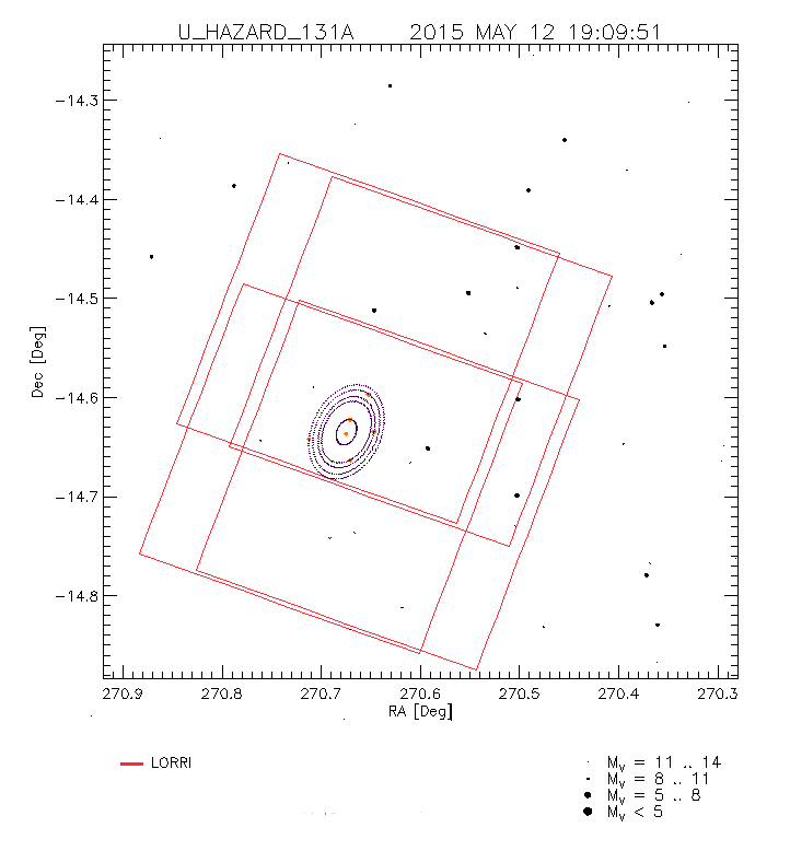
Figure 5: The footprint on the sky typical for most of the $2\times 2$ LORRI mosaics used for back-scattered light searches is shown. This example is from the U_HAZARD_131A sequence, which occured at P$-64.$ Note that the mosaic is aligned with and elongated along the projected major-axis of the orbits of the minor satellites. There is a small-scale random pattern in the relative positioning of the four LORRI fields due to accuracy limits in the absolute positioning of the spacecraft.

Figure 6: The first $4\times 4$ LORRI image, lor_0296651467, in the P$-29$ hazard-search sequence is shown to exhibit the typical features present in the search imagery. The exposure is 10s. Note the heavily crowded background from the Milky Way bulge. Hot pixels and cosmic-ray events are also evident. Pluto and Charon are both heavily overexposed. The vertical streaks spanning the full frame are charge left over from an incomplete frame-transfer correction due to the saturated centers of Pluto and Charon. Both objects, as well as the brightest stars, also exhibit “amplifier undershoot” tails to the right of the core of the images, which pull the local signal below the sky level.

The hazard search comprised seven epochs of observations, each divided into two or three sequences or sub-epochs of imaging, separated by a few hours to a day, to enable the detection of satellites by their orbital motion. In each sub-epoch, a $2\times 2$ mosaic of heavily-overlapping LORRI fields covered the region around Pluto (Figure 5). We set the orientation to align with the projected major-axis of the satellite system in the CCD y-direction. At each position in the mosaic, we obtained multiple 10s exposures. For most of the epochs, we obtained images at each position using two roll angles of the spacecraft separated by $90^{\circ}$. This made it possible to mitigate the obscuration of portions of the field by the strong diffraction spikes, incompletely corrected charge-transfer smearing in the column direction, and “amplifier undershoot” trails in the row direction produced by the disks of Pluto and Charon, which were severely over-exposed in all sequences. The detailed number of exposures, as well as the temporal sampling intervals, varied over the hazard sequences. The deepest search occurred at P$-29$ (29 days prior to closest approach to Pluto) with 24 images at each of the four mosaic positions for each of four sub-epochs.

3.2 Reduction and Analysis of the Observations

Reduction of the hazard images to effect the detection of faint satellites and rings presented a strong technical challenge to the NH team. During the approach phase, Pluto was seen in projection against the bulge of the Milky Way, thus the background was richly crowded with stars. The images were $4\times 4$ binned to achieve maximum photometric sensitivity to point sources (as well as greatly reducing the downlink data volume), but as a result were severely under-sampled. The NH pointing system was optimized for the short integrations needed during the closest phases of the encounter; because the spacecraft does not have reaction wheels for fine pointing control, the spacecraft attitude typically drifted slightly during the 10s exposures, though drift was minimized by firing thrusters to maintain pointing within a narrow (arcsecond-class) deadband. As such, the PSF of the images could vary markedly from exposure to exposure. Lastly, the images were also strongly affected by cosmic-ray events. We show a typical hazard-search LORRI $4\times 4$ 10s image in Figure 6. Note the heavily crowded background. In a single image the completeness limit is about $m_{V}\sim 18,$ going to $m_{V}\sim 20$ in the complete stack at any epoch. A deep image of the full search area is shown in Figure 7.

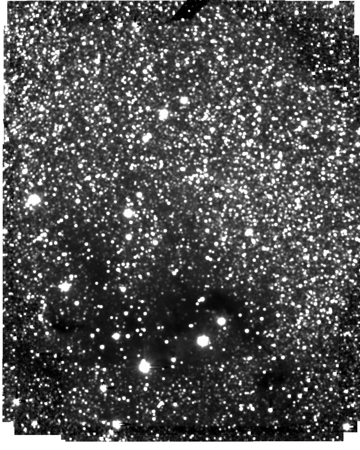
Figure 7: For reference we show a deep stack of 340 LORRI $4\times 4$ images covering the complete hazard-search area. The images were drawn from the sequences in Table 2 with encounter dates P$-63$ and earlier. Pluto was present in the field, but was masked out using its proper motion over the time span of the image set.

Eight members of the NH team examined all of the hazard images. The experience of this team was considerable and diverse, encompassing work on crowded stellar fields in ground-based, HST-based, planetary, and even extra-galactic contexts. As such, the team deployed a diversity of analysis approaches. Broadly speaking, the search task could be broken down into three parts. The first step typically focused on a way to model or remove the strongly-crowded, but largely invariant stellar background of the images. The resulting difference images at a common sub-epoch, rotation, and position within the larger search field, would then be aligned and stacked using various statistical procedures to eliminate left-over residuals from bright stars, cosmic rays, hot pixels, and so on. Lastly, stacked images at different sub-epochs would be compared to search for faint satellites or rings (see Figure 8). The central concern in all approaches was to take care to preserve large-scale diffuse features indicative of rings, or transient stellar point sources indicative of possible unknown satellites. We briefly describe the various strategies.

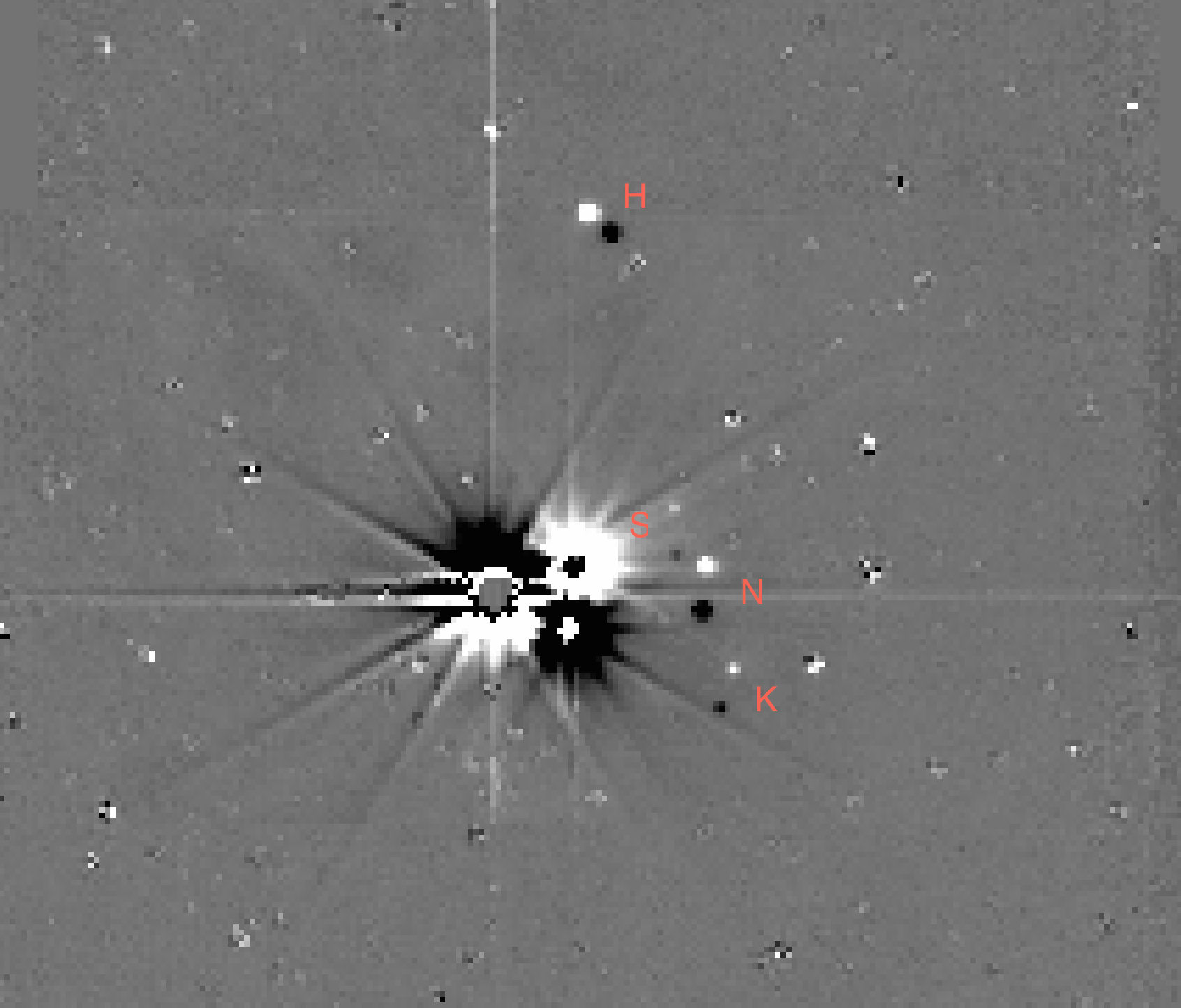
Figure 8: A demonstration of the search for faint satellites with the P$-39$ hazard sequences. After subtracting the stellar background using the principal components analysis method stacks are made at two P$-39$ sub-epochs separated by 17 hours, which are subtracted form each other. The known satellites, Hydra, Nix, Styx, and Kerberos (indicated by their initials) are readily recognized by their motion between the two sub-epochs. The strong residuals at the center are due the the motion of Pluto (L) and Charon (R) with respect to the barycenter as well.

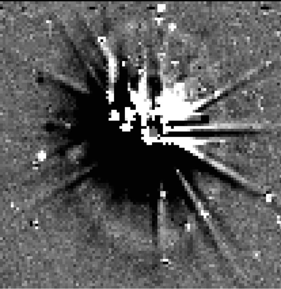
Figure 9: Recovery of a simulated ring associated with Styx and having $I/F=2\times 10^{-7}.$ In this test the ring was recovered by differencing image stacks generated from simulations of the three U_HAZARD_149 and three U_HAZARD_156 sequences obtained on P$-46$ and P$-39$. The P$-39$ ring image is angularly larger and is subtracted from the P$-46$ image, creating a difference ring image that is negative (dark) on the outside and positive (lighter) on the inside. The simulated image of Styx (positive in P$-46$) is seen embedded in the ring at the top of the image and slightly right of center. Pluto and Charon are strongly over-exposed. In this simulation, while the stellar background was well modeled, no attempt was made to model Pluto or Charon in this particular case.

One approach was to characterize the image PSF and pointing variations at any location with principal components analysis (PCA) applied to the background reference image sets. The PCA approach generated a set of “eigenimages” that encapsulated the image-to-image variations within the reference set (Boroson & Lauer, 2010). This allowed a construction of a model reference image for each image in the actual hazard sequences that attempted to match the specific PSF and pointing for the image modeled. Subtracting each model image from each search image produced a set of difference images at each search location and epoch that were then stacked to build up the signal for faint satellites and rings. This process was done in a few iterative cycles, rebuilding the initial models in one cycle based on sources rejected in a previous cycle. Crucially, the stacking included statistical rejection of cosmic-ray events and other variable defects. Once the stacks were completed, rings and faint satellites would be identified by comparing the stacks made at different epochs.

A second approach used various models of the stellar background based on stacks either generated from the reference sequences obtained in advance of the hazard-search, or from other hazard-search epochs than the one being searched, depending on whether the goal was to detect satellites versus rings in the search imagery. A key step in all cases was to include models of the light distributions produced by Pluto and Charon, including their associated optical ghosts, models of the frame transfer smear for the Pluto and Charon images, and a model that reproduces the “jailbar” pattern seen in the raw images. All the model-subtracted images taken at a single pointing and roll angle were combined using a robust mean technique to produce a deep composite image, with most of the original image artifacts removed.

Yet another approach took advantage of the fact that, by random chance, certain image pairs would occasionally have very similar PSFs. This procedure cross-correlated every pair of ring search images and, for each image, and used the “most similar” subset of the remaining images to model and subtract out the star field. Again, after the subtraction, the resulting difference images were stacked using robust statistics to reject cosmic rays and other variable defects.

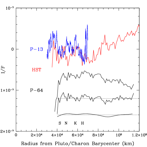
Figure 10: Back-scattering $I/F$ radial brightness profiles covering the the orbital range of Pluto’s minor satellites are shown. The orbital radii of the satellites are indicated by their initials. The present results measured from LORRI hazard-search images are labeled with the P$-64$ and P$-13$ sequence labels. A strong centrally-increasing scattered-light background has been subtracted from the P$-13$ profile to improve the identification of narrow rings. “HST” indicates the final coadded HST I/F profile derived in the previous section and presented in Figure 4. The P$-64$ $I/F$ profile has the smoothest background of the various hazard-search epochs, but has an average level of $I/F=-7\times 10^{-8}.$ Profiles derived by subtracting a parabolic background from the P$-64$ observed $I/F$ profile; and then smoothing it to $1.2\times 10^{4}$ km resolution ($8\times$ the native resolution) are shown below the original P$-64$ profile.

3.3 Limits on Rings, Debris, and Dust From Back-Scattered Light

The mission-critical importance of the hazard search engendered a formal process to demonstrate optimal analysis strategies well in advance of the encounter. All search methodologies were tested with extensive high-fidelity simulations of all the search sequences, which included simulated rings and satellites that had a wide range of apparent surface brightnesses and luminosities. The predicted sensitivity limits on the detection of rings were based on rings injected into these simulations. Interestingly, despite the diversity of the analysis techniques, all reached similar levels of sensitivity. As an example, simulated rings close to Pluto with normal $I/F=2\times 10^{-7}$ were readily identified (Figure 9). It’s clear that fainter rings than this example would still be readily detected. As discussed below, however, actual $I/F$ detection limits are determined by direct analysis of the observations; we did not validate the simulations to serve this purpose.

Instead, we derived upper limits on normal $I/F$ for the ring intensities in the actual encounter hazard-search from our analysis of the residuals in the deep stacked images at any epoch. Using the known geometry of the observations (i.e., the spacecraft location relative to Pluto and the geometry of the Pluto system), we created “backplanes” for each composite image composed of ($r$, $\theta$) pairs of coordinates for each pixel, where $r$ is the radial distance of the pixel from the barycenter of the Pluto system in the satellite orbital plane, and $\theta$ is the azimuthal angle of the pixel from the reference longitude, also calculated in the satellite orbital plane. Points at a fixed distance from the Pluto barycenter form a foreshortened ellipse in the sky plane (i.e., in the camera image plane). Assuming that any ring-like structure can be approximated by such a figure, the sensitivity for ring searches is greatly enhanced by averaging, or calculating the median of, the pixel intensities over all azimuths as a function of distance from the barycenter. Some example radial profiles using these azimuthal averages (or medians) are displayed in Figure 10. Although our primary focus was on the region outside the orbit of Charon, we also sought rings and small moons orbiting interior to Charon. For that study, the analysis procedure was the same except that the backplane values of ($r$, $\theta$) were measured from the center of Pluto rather than from the system barycenter.

Contrary to our original expectations, we found that the most sensitive ring search was derived from the first epoch of observations, which occured at P$-64.$ As the spacecraft drew closer to the Pluto system, the intensities of the barely resolved Pluto and Charon images grew faster than the surface brightness of any diffuse (i.e., resolved) structures. The scattered light and ghosts from the highly saturated Pluto and Charon images produced bright and spatially complex backgrounds, which complicated our attempts to detect faint rings or diffuse debris as the spacecraft moved closer to Pluto (see Figure 11).

For the azimuthally averaged spatial brightness profiles, we converted from instrumental units to $I/F$, a commonly-used surface brightness parmeterization, at the LORRI pivot wavelength (6076 Å) using:

$$I/F=C/\texttt{RSOLAR}\times\pi R_{\rm AU}^{2}/F_{\sun}$$ (3)

where $C$ is the count rate in DN/s, $\texttt{RSOLAR}=4.092\times 10^{6}~{}{\rm DN/s}~{}({\rm erg~{}cm^{-2}~{}s^{-1}~{}\AA^{-1}~{}sr^{-1}})^{-1}$ is the relevant LORRI photometry calibration constant, and $F_{\sun}$ is the solar flux, 176 erg cm^-2 s^-1 ${\rm\AA^{-1}}$ at the LORRI pivot wavelength at 1 AU. To convert to normal $I/F$, we used New Horizons’ nearly fixed emission angle $e=43\hbox to1.0pt{}\hbox to0.0pt{${}^{\circ}$\hss}.\hbox to2.0pt{}2$

A radial brightness profile from the first epoch of the P$-64$ hazard-search is shown in Figure 10. Scattered light strongly affects the profile inside Styx’s orbit ($r_{S}=42$,413 km), but the profile is essentially constant at $\sim$ $-7\times 10^{-8}$ for larger radial distances covering the orbits of the minor satellites and extending out to twice the orbit of Hydra. The residual $I/F$ values are negative because the background for the reference template image (obtained a year earlier) is systematically larger than the background for the P$-64$ observations. We conclude that this constant offset of $-7\times 10^{-8}$ represents a conservative upper limit for any large scale distribution of dust or debris that would represent a constant background of the scale of the LORRI field at P$-64$ ($\sim 10^{5}$ km).

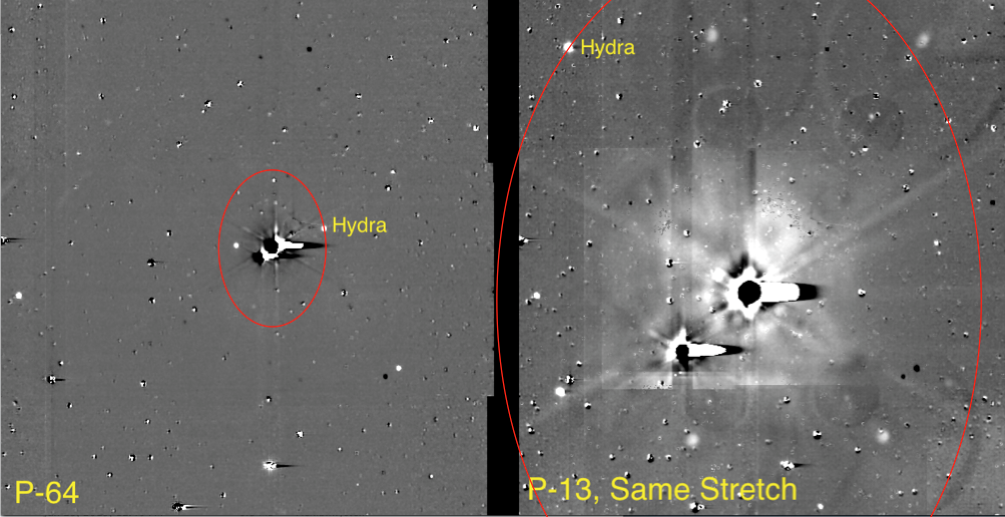
Figure 11: Image stacks are shown for the P$-64$ and P$-13$ sequences at the same stretch to show the increased effects of scattered light from Pluto and Charon for the later sequences. The red ellipse indicates the orbit of Hydra. In each case, non-variable stars have been subtracted using an image stack taken a year earlier, and models of Pluto Charon, incorporating large-angle PSFs and optical ghosts, have been subtracted as well as possible, given model limitations. This treatment can be contrasted with that in Figure 9, which still includes the residual images of Pluto and Charon.

Narrow or even broad rings of finer scale, however, should be evident as compact positive excursions in the $I/F$ profile. To establish limits on such features, we fitted and subtracted a smooth background from the P$-64$ profile for $4\times 10^{4}~{}{\rm km}<r<1.2\times 10^{5}~{}{\rm km}$, and measured the mean residuals on different spatial scales. The background-subtracted P$-64$ profile, which now has zero mean, is plotted below the input P$-64$ profile in Figure 10. At the $1.5\times 10^{3}~{}{\rm km}$ resolution limit of the profile, the $3\sigma$ limit on any detectable ring is $I/F\sim 2\times 10^{-8}.$ This decreases to $I/F\sim 1\times 10^{-8}$ on $6\times 10^{3}~{}{\rm km}$ scales and $I/F\sim 7\times 10^{-9}$ on $1.2\times 10^{4}~{}{\rm km}$ scales. The background-subtracted P$-64$ profile, smoothed to $1.2\times 10^{4}~{}{\rm km}$ resolution is shown as the bottom trace in Figure 10. These limits are $\sim 4\times$ fainter than the HST limit over the same region.

The spatial profiles on the later dates have much higher scattered light levels, as illustrated for P$-13$ in Figure 10. The strongly sloping background and high absolute brightness levels makes these images much less sensitive to rings or debris. Even after fitting a smooth curve to the sloping background, the residuals are much larger for P$-13$ versus P$-64$ (Figure 11).

4 Searching by Stellar Occulations

Near the time of closest approach we also searched for rings, debris, and dust clouds by the occultation of starlight using the Alice instrument, New Horizons’ ultraviolet (UV) imaging spectrometer (Stern et al., 2008). These sequences are detailed in Table 2. Alice was ideal for stellar occultations of UV-bright stars because of its ability to take sustained high-cadence observations. Its primary aperture (the ‘Airglow’ entrance) admits light through a 40 mm diameter aperture. The projected field-of-view (FOV) is in the shape of a ‘square lollipop’, with a $2^{\circ}\times 2^{\circ}$ square adjoining a $4^{\circ}\times 0\hbox to1.0pt{}\hbox to0.0pt{${}^{\circ}$\hss}.\hbox to2.0pt{}1$ rectangle. The focal plane has 32 rows (spatial) $\times$ 1024 columns (spectral). Alice’s data is delivered as a list of individual photons, each tagged with a row, column, and time. The instrument observes continually, with negligible readout time.

We used Alice for four occultation searches during the Pluto encounter. The idea of these observations was to search for ring dust or orbital debris along the line-of-sight between NH and a distant star. The theoretical resolution limit is set by the Fresnel limit, $r_{F}=\sqrt{D\lambda/2},$ which gives the scale of the smallest resolvable feature in an occultation, where $D$ is the distance to the occulting body, and $\lambda$ is the effective wavelength, which for Alice is $\sim 150$ nm.

For each observation, Alice pointed constantly at a fixed RA/Dec such that the bright target stars were kept centered on one Alice pixel during the entire sequence. As NH traveled on its trajectory, portions of the Pluto system passed between the stars and the spacecraft. Alice operated continually, allowing the line-of-sight optical depth to be measured for the duration of the occultations.

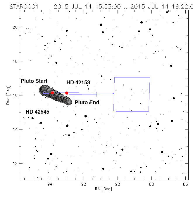
Figure 12: Geometry of Alice occultation in the Pluto-Charon, for the Alice_StarOcc1 sequence. The blue outline represents the Alice slit.

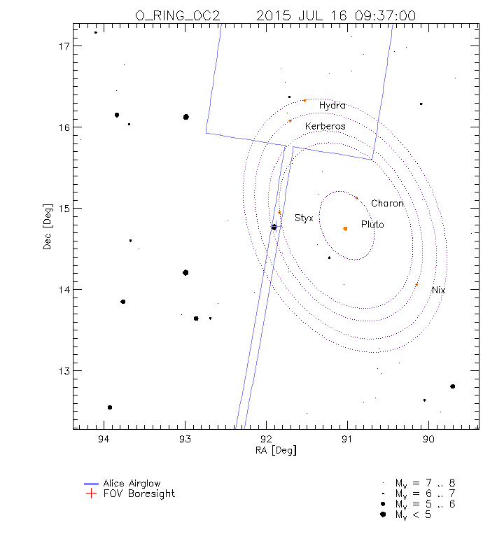
Figure 13: Geometry of the O_Ring_Oc2 occultation of the region of Nix’s orbit.

The first set of occultations (Alice_StarOcc1, Figure 12) was observed starting approximately 4 h after the closest approach to Pluto. Alice monitored two bright stars, which were placed in the slit simultaneously, allowing two different occultations to be measured with one sequence. The observation lasted 2.5 h, and Alice data was read out at 250 Hz, resulting in $2.25\times 10^{6}$ independent spectral images. The first star’s projected distance ranged from $0.5r_{\rm P}$ to $1.9r_{\rm P}$ (600–2260 km) from Pluto’s center, where $r_{\rm P}=1188.3\pm 1.6$ km is Pluto’s radius (Nimmo et al., 2017). (i.e., a full Pluto occultation), while the other covered an appulse spanning $1.5r_{\rm P}$ to $2.5r_{\rm P}$ (1800–3000 km). The projected velocity varied due to the rapidly changing geometry, but was typically 0.5 km/s to 1 km/s, giving us meter-scale sampling in many cases. The Fresnel limit $r_{F}$ was 4-5 m. Additional details of the observing geometry are given in Table 3.

Table 3: Alice stellar occultation geometry. Distances are projected distance from star to Pluto center.

			Projected
			Velocity	Inner	Outer
Sequence	Start	Inner	[km/s]	[km]	[km]	Tilt	Star
Alice_StarOcc1	2015 Jul 14 15:53 - 18:23	9000.0 s	0.79	322	6,111	$45\hbox to1.0pt{}\hbox to0.0pt{${}^{\circ}$\hss}.\hbox to2.0pt{}6$	HD 43153
”	”	”	0.66	2,411	6,858	$45\hbox to1.0pt{}\hbox to0.0pt{${}^{\circ}$\hss}.\hbox to2.0pt{}6$	HD 42545
O_Ring_Oc2	2015 Jul 16 09:37 - 10:37	3600.0 s	0.39	46,794	48,185	$43\hbox to1.0pt{}\hbox to0.0pt{${}^{\circ}$\hss}.\hbox to2.0pt{}4$	67 Ori
O_Ring_Oc3	2015 Jul 16 21:25 - 22:24	3593.4 s	0.39	63,233	64,625	$43\hbox to1.0pt{}\hbox to0.0pt{${}^{\circ}$\hss}.\hbox to2.0pt{}4$	67 Ori

The inner Pluto-Charon region probed by these occultations was particularly interesting because it sampled the region where dust grains can survive for at least $10^{4}$ Pluto-Charon rotation periods (or 175 years) (Giuliatti Winter et al., 2013). Kammer et al. (2016) have analyzed this data set to probe Pluto’s atmospheric structure; we use the data far enough from Pluto that it is not affected by atmospheric refraction.

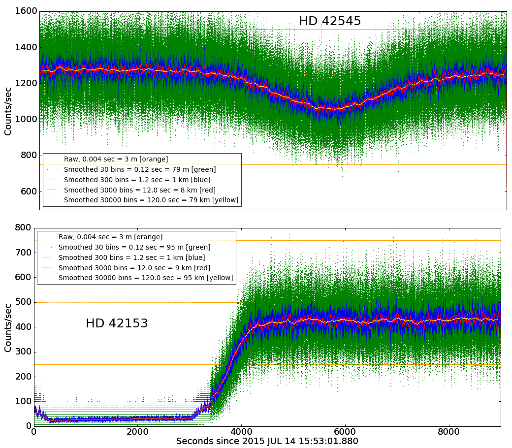
Figure 14: Light curves from the Alice occultations of the Pluto-Charon region, both taken in the Alice_StarOcc1 sequence. The orange points (which appear as discrete horizontal lines due to their low individual DN values) are the raw observations at 250 Hz, and the other curves are binned to larger spatial scales. The broad dips are due to the appulse and occultation of Pluto.

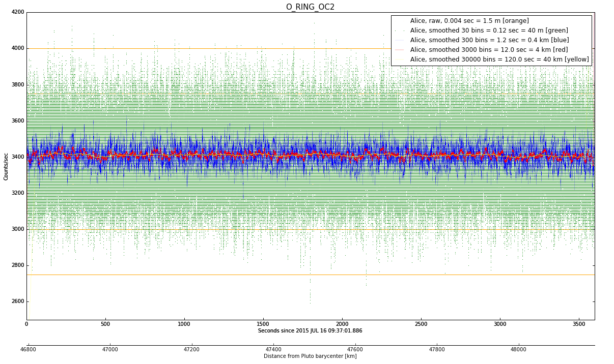
Figure 15: Alice occultation in the Nix region, O_Ring_Oc2. The curve for O_Ring_Oc3 is similar, but is not shown.

The second and third occultations occurred approximately two days after the Pluto encounter. These sequences — O_Ring_Oc2 and O_Ring_Oc3 — probed the region around the orbits of Nix and Hydra, respectively, where collisional debris from these bodies might be found (Figure 13). Dynamical studies show that dust in these regions can be stable for at least $10^{5}$ Pluto rotation periods (1,750 years) (Giuliatti Winter et al., 2013). Because these observations were taken later during the encounter, their projected speeds are much lower ($\sim 0.37$ km/s), and the radial width covered by each scan is just slightly over $1r_{\rm P}$ (1188 km). Typical Fresnel resolution $r_{F}$ was $\sim 10$ m, and per-sample resolution at 250 Hz was 1.5 m.

We analyzed all these Alice occultations in the same way. We started with the raw ‘pixel list’ data, which enumerates all photons received during the occultation, time-tagged to 4ms resolution. We used this information to extract a light curve, incorporating only the photons received on the appropriate rows corresponding to the target star location. We summed spatially over three rows. We then binned photons at all wavelengths, omitting 20 adjacent columns which were contaminated by interplanetary H Ly-$\alpha$ emission near 1216 Å. The remaining signal was the light curve $I(t)$. The typical count rate was 400–3400 DN/s, depending on the target star.

Stellar flux during Alice_StarOcc1 was affected by vignetting as the slit’s sky position moved within its $0\hbox to1.0pt{}\hbox to0.0pt{${}^{\circ}$\hss}.\hbox to2.0pt{}035\times 0\hbox to1.0pt{}\hbox to0.0pt{${}^{\circ}$\hss}.\hbox to2.0pt{}035$ box. This motion by the spacecraft’s guidance system was not enough to move the star off the pixel, but did reduce the flux by about 50% at the extremes of motion. We corrected for this by dividing the light curve $I(t)$ by a simple linear vignetting model based on the spacecraft’s pointing in declination. Vignetting in the RA direction was negligible.

The per-sample resolution of these observation is below the Fresnel limit. We therefore binned the data using boxcar smoothing, to search for occultations on a variety of scales from 10 m - 100 km. Binning allowed us to search for individual bodies at meter scales, in addition to extended clouds or rings of material at larger spatial scales. Light curves from the Alice occultations are shown in Figs. 14-15.

The optical thickness of a ring can be computed by comparing the flux at each timestep $F$, to the mean flux $F_{0}$,

$$F=F_{0}\ \exp(-\tau/\mu),$$ (4)

Usually we refer to the normal optical thickness $\tau_{n}$, where $\tau_{n}=\tau\mu$. Our limits on optical depth are given in Table 4. We did not find any statistically significant features in any of the four occultation curves. At the fine-resolution limit, Alice would have detected individual bodies of size 5-10 meters; it detected none along its path. When binned at larger resolutions, the data would have easily detected a Chariklo-type ring (Braga-Ribas et al., 2014) in the Pluto system ($\tau=0.4$, width = 5 km), but such a feature was not seen. Binned to low resolution, Alice’s limit of $\tau_{n}<0.006$ at 40 km does not exclude the existence of a Jupiter-type ring at Pluto, although such a ring was ruled out by the LORRI and MVIC imaging data described elsewhere in this paper.

Table 4: Alice optical depth limits from stellar occultations.

Sequence	Resolution	$\tau_{n}$
O_Ring_Oc2; O_Ring_Oc3	$r_{F}=11$ m	$<$0.3
	50 m	$<$0.1
	500 m	$<$0.03
	5 km	$<$0.01
	50 km	$<$0.003
Alice_StarOcc1	$r_{F}=4$ m	$<$0.43
HD 42545	0.08 km	$<$0.20
	0.8 km	$<$0.065
	8 km	$<$0.028
	80 km	$<$0.0080
Alice_StarOcc1	$r_{F}=4$ m	$<$0.24
HD 42153	0.1 km	$<$0.14
	1 km	$<$0.049
	10 km	$<$0.024
	100 km	$<$0.0090

Together these occultations explored only about 15% of the total radial extent between Pluto and Hydra. Our integration length was limited by the spacecraft’s downlink scheduling and Alice’s relatively large data volume. The imaging data covered this region and others completely, although at lower resolution than Alice’s finest limit.

5 Direct Detection of Dust Impacts

The Student Dust Counter (SDC) onboard NH was designed to directly detect the impact of dust particles (Horányi et al., 2008). SDC measures the mass of dust grains in the range of $10^{-12}<m<10^{-9}$ g, covering particle radii of approximately 0.5 to 10 $\mu{\rm m}.$ A period of $\pm 5$ days centered on Pluto closest approach, corresponding to approximately $\pm 5000r_{\rm P}$ ($5.9\times 10^{6}$ km) was used to evaluate the dust density near Pluto. Throughout this entire period, SDC recorded only a single event that could be attributable to a dust impact (Bagenal et al., 2016).

During the Pluto encounter, propulsive spacecraft attitude maneuvers executed by New Horizons introduced excessive noise to the SDC detectors. To avoid recording this noise, SDC was set to a charge threshold of $Q=10^{7}e^{-}$ (where $e^{-}$ is the electron charge), corresponding to a smallest detectable particle radius of $\sim 1.5~{}\mu{\rm m}.$ From the amplitude distribution of all recorded noise events near Pluto encounter, it was determined this event was above the $2\sigma$ error threshold of SDC noise events within $\pm 5000r_{\rm P}.$ Hence, the probability that this event was due to a true dust particle impact was estimated to be $\sim 95\%.$

As described in Bagenal et al. (2016), this event was used to define an upper limit for the dust density within $5000r_{\rm P}$ for grains larger than 1.4 $\mu{\rm m};$ from this calculation we found the dust density for particles larger than 1.4 $\mu{\rm m}$ to be $\sim 1.2~{}{\rm km^{-3}}.$ A 90% confidence level for the dust density in this region of space was calculated to be in the range $0.6<n<4.6~{}{\rm km^{-3}}.$ However, we caution that our single candidate particle impact occurred at a distance of $\sim 3070r_{\rm P}$ ($3.65\times 10^{6}$ km). This great distance, combined with (1) the fact that the spacecraft was then very far above the equator plane and (2) that no other particle impacts were detected closer or in this plane, make it unlikely that this particle is associated with rings or other coherent dust structures in the Pluto system. Further, within the error bars the densities at the high threshold setting of SDC (1.4 $\mu$m radius) before, during, and after the encounter remained the same (2015-2017), indicating the detection near Pluto was likely not special. We conclude that this particle was most likely a background interplanetary dust particle from the Kuiper Belt.

6 Searching by Forward-Scattered Light

6.1 Design of the Observational Program

After closest approach, New Horizons looked back at the Pluto-Charon system at several epochs to search for faint dust rings through forward-scattered sunlight. Both LORRI and the Multi-spectral Visible Imaging Camera (MVIC), a component of the Ralph remote sensing package, were used to generate deep image-mosaics covering a large angular area of the sky centered on Pluto. The forward-scattering observation sequences for both LORRI and MVIC are listed at the bottom of Table 2. LORRI was described in $\S\ref{sec:back}$ in the context of looking for rings in back-scattered sunlight. In brief, MVIC comprises a set of narrow strip-format CCDs with various band-passes. For the ring search, we used the MVIC panchromatic (Pan-Frame) CCD, which is a $5024\times 128$ pixel array used in white-light (400 - 975 nm bandpass) at the focus of a 7.5 cm off-axis reflector. Unlike the other MVIC CCD channels, which scan over the field of view using time-delay integration, MVIC Pan-Frame uses a standard frame-transfer CCD. The pixel scale is $4\hbox to1.0pt{}\hbox to0.0pt{${}^{\prime\prime}$\hss}.\hbox to2.0pt{}1,$ yielding a $5\hbox to1.0pt{}\hbox to0.0pt{${}^{\circ}$\hss}.\hbox to2.0pt{}7\times 0\hbox to1.0pt{}\hbox to0.0pt{${}^{\circ}$\hss}.\hbox to2.0pt{}15$ field. See Reuter et al. (2008) for further details.

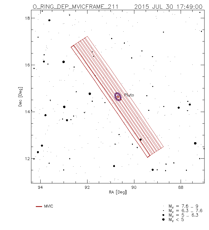
Figure 16: The footprint on the sky for the O_RING_DEP_MVICFRAME_211 MVIC forward-scattered light search on P$+16.$ Note that the mosaic is aligned with and elongated along the projected major-axis of the orbits of the minor satellites. The same footprint is also used for the P$+7$ and P$+110$ searches.

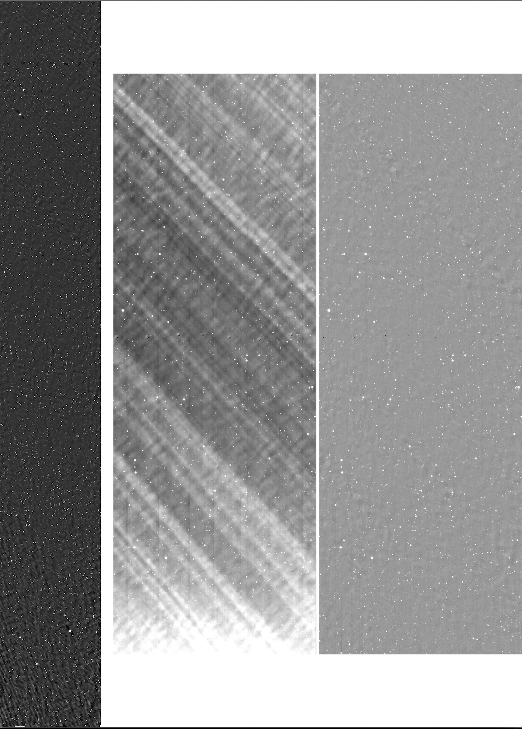
Figure 17: Left: The complete reduced stack of the P$+110$ MVIC outbound mosaics. The field covered is $5\hbox to1.0pt{}\hbox to0.0pt{${}^{\circ}$\hss}.\hbox to2.0pt{}7\times 0\hbox to1.0pt{}\hbox to0.0pt{${}^{\circ}$\hss}.\hbox to2.0pt{}8$. Middle: The central portion of the first day-P$+110$ mosaic zoomed by $2\times$ to show the strong stray sunlight pattern. Right: The same region corrected for stray light.

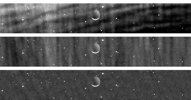
Figure 18: Image reduction demonstrated for a single image taken from the MVIC outbound mosaic O_RingDep_A_1. Top: The central portion of the image within the mosaic that included the “nightside” hemisphere of Charon. The strong mottling pattern is due to stray sunlight entering the camera. Middle: The first reduction step is to remove the average pattern seen in at all images within the mosaic. Bottom: The second reduction step is to remove the streaks that traverse the entire mosaic. Note the recovery of “Pluto shine” on the upper right portion of the dark hemisphere of Charon.

In general design, the LORRI and MVIC searches have strong similarities. Both instruments were used within an hour of each other at given epoch and covered roughly similar areas. Further, as was done for the hazard searches, LORRI was again used with $4\times 4$ binning to maximize sensitivity and minimize telemetry; as such the LORRI and MVIC pixel scales were nearly the same. Apart from an initial search conducted using MVIC only a day after closest approach, joint LORRI and MVIC searches were conducted at days P$+7,$ P$+16,$ and P$+110.$ The final epoch extended the search to the full Hill sphere surrounding Pluto, where $r_{\rm Hill}=6.4\times 10^{6}~{}{\rm km}$ at Pluto ($99.3\times$ the orbital radius of Hydra, for comparison). The phase angle was nearly constant at $\sim 165^{\circ}$ over all epochs, and the close angular proximity of the sun introduced strong stray light into both cameras. The MVIC searches, however, were nearly two orders of magnitude more sensitive than those done with LORRI due to the much smaller effects of stray light in MVIC, plus the longer integrations done with this instrument. We detail the LORRI and MVIC sequence designs further in the next two subsections.

6.2 The MVIC Mosaics

6.2.1 Observation and Preparation of the MVIC Mosaics

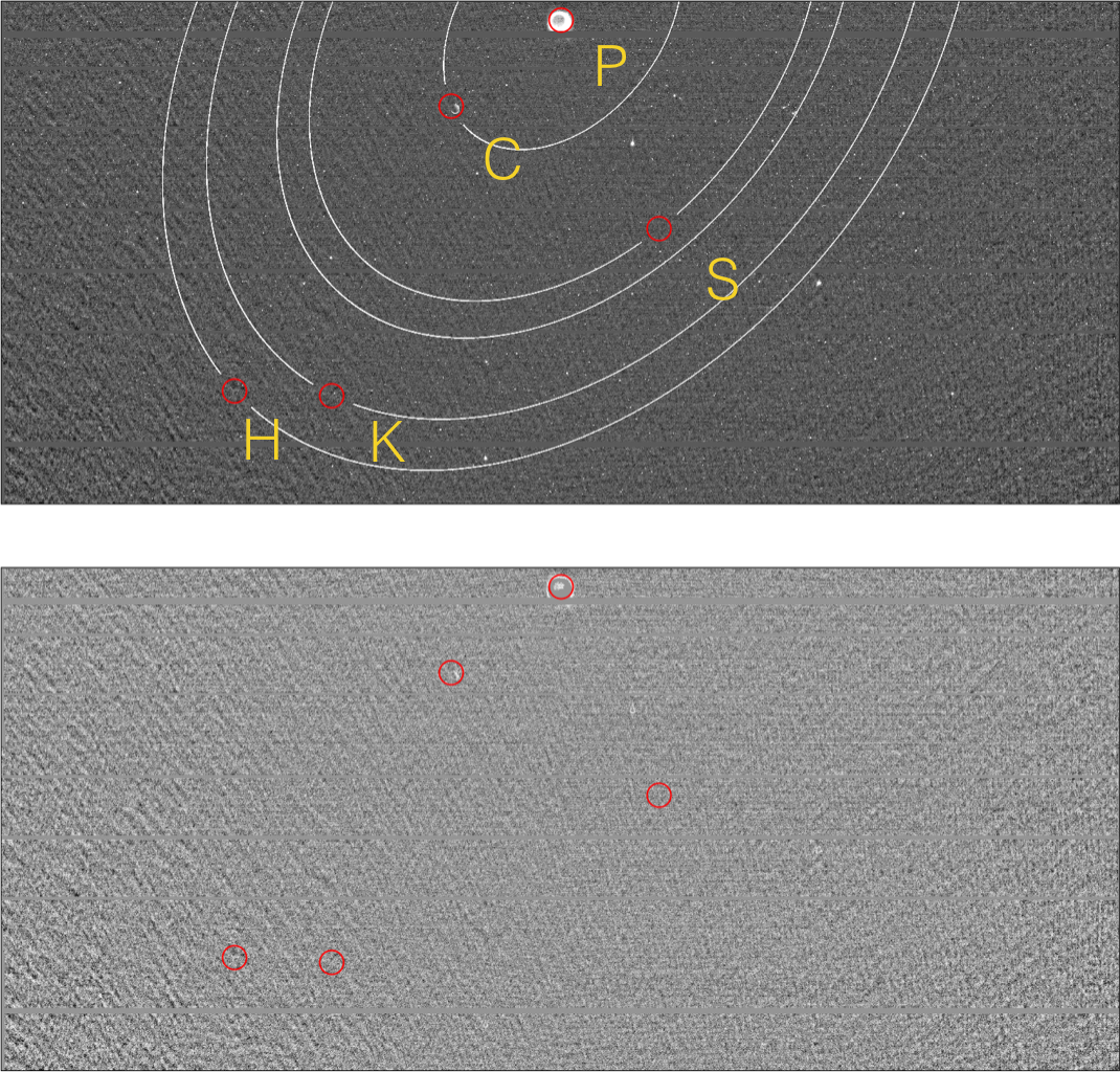
Figure 19: MVIC outbound mosaic O_RingDep_A_1, taken at P+4 h. Top: MVIC mosaic, stray-light-subtracted, with orbits of Pluto system indicated (P=Pluto, and so forth). Bottom: Same as top, but with rescaled with bright pixels removed so as to reveal any structure in the background image.

The MVIC forward-scattering ring search sequences benefit from markedly longer exposure times that go far beyond compensating for the smaller aperture of Ralph as compared to LORRI, a markedly lower amplitude of stray sunlight, and fortuitously, a pattern of stray light that is considerably easier to remove. The approach to constructing the MVIC mosaics was to align the long axis of the CCD with the projected major axis of the satellite orbits, using spacecraft pointing to tile the field in the minor-axis direction (Figure 16). For the P$+7,$ P$+11,$ and P$+110$ mosaics, images were obtained at 7 pointings along the minor-axis of the projected orbital plane, with $25\times 10$s exposures obtained at each location, for a 250s total exposure. The reduced P$+110$ mosaic is shown in Figure 17, as well as a central portion of it before and after the stray sunlight was corrected for. The exposures were split into separate sequences of 20 and 5 exposures, with a small offset of a few pixels between the two. The images at any position also overlapped slightly with those at flanking positions. For the P$+110$ search, as with LORRI, the full mosaic was done three times for 750s total exposure. The first MVIC search, obtained a day after close approach, comprises 17 pointings along the projected minor axis, with $15\times 10$s exposures or 150s total at each. This mosaic is offset, with Pluto positioned near the edge in the minor axis direction, and the spacing of some of the pointings is such that the images do not overlap, leaving gaps in portions of the mosaic.

Stray sunlight affected the MVIC images, but at a lower level and with less highly variable structure than was seen in the LORRI images. Examination of the complete ensemble of MVIC images for a given mosaic showed that the stray light pattern could be decomposed into a constant component that was present in all images, and a pattern of streak or rays that appeared to be fixed in space. The constant component could be visualized by averaging the images, although in practice we isolated it by a PCA analysis of the ensemble, iteratively rejecting stars from affecting the extraction of the component (cosmic rays were easily identified and repaired from the multiple images available at each position). Once derived, the constant component could be subtracted from all images in the ensemble, leaving the pure streak-pattern behind. Looking at a complete mosaic, it was clear that the streaks appeared to be radiating from a point on the sky (although this was not the projected location of the sun). The streaks were then removed with an ad hoc algorithm that smoothed along radial lines emanating from the streak radiant. The smoothing length was $\sim 80$ pixels and the operation was conducted on the mosaiced images with stars clipped out. These reduction steps are demonstrated Figure 18.

6.2.2 Ring limits from the MVIC Observations

An example of the processed MVIC ring mosaics is shown in Figure 19. Here ${\rm R_{\rm H}}$ refers to the distance of Hydra from the system barycenter, 64,738 km. No rings are obvious in the mosaics. But planetary ring structure can often exist at levels that are not easily visible to the eye, and in many cases they can be seen when many pixels are summed appropriately (e.g., Showalter & Cuzzi, 1993; Throop & Esposito, 1998). We used this technique to search quantitatively for faint rings that might be unseen to the eye.

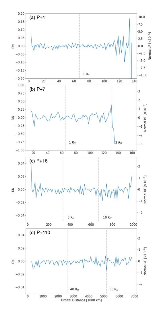
Figure 20: Radial profiles from the MVIC mosaic at (a) P$+1$, (b) P$+7$, (c) P$+16$, and (d) P$+110$. Pixels are binned by radial distance from the system barycenter, using N=100 radial bins. No ring structure is apparent. The larger scatter at the extreme inner and outer regions is due to larger errors in the stray-light correction at the margins of the detector and is not significant.

We first registered the full mosaics precisely based on the known positions of field stars. This corrected for the several-pixel uncertainty in our NH pointing knowledge. Based on the measured pointing, we then generated backplanes for the images, where for each pixel we computed a value for the projected radial distance and azimuth angle, referenced relative to a plane centered on Pluto and normal to Pluto’s pole (Seidelmann et al., 2007). We performed a two-pass removal of any bright pixels with flux exceeding $3\sigma$ above the median, which were typically due to stars or known bodies in the Pluto system. We then grouped pixels by radial distance, and computed the mean within each bin. We used both N=100 and N=1000 radial bins, spaced linearly from zero to the maximum radial distance in each mosaic. Radial profile $I/F$ profiles from all four epochs of MVIC observations are shown in Figures 20a to 20d.

The radial profiles did not reveal any features that were clearly indicative of rings or arcs. There were no features that appeared aligned with the projected geometry of the Pluto system. All visible structures in the images appeared to be associated with either stray light, or the edges of our mosaic scan pattern.

Our radial profiles can be used to place quantitative upper limits on ring material at Pluto. We first converted from DN to $I/F$ using the instrumental calibration constant RSOLAR:

$$I/F=C\,/\,\texttt{RSOLAR},$$ (5)

where $\texttt{RSOLAR}=9.8813\times 10^{4}{\rm DN/s}~{}({\rm erg~{}cm^{-2}~{}s^{-1}~{}\AA^{-1}~{}sr^{-1}})^{-1}$ for MVIC’s Pan-Frame sensor, and $C$ is the count rate in DN/s. As before, the solar flux at the MVIC Pan Frame pivot wavelength ($\lambda$ = 6920 Å) was taken to be $F=145{\rm~{}erg~{}cm^{-2}~{}s^{-1}~{}\AA^{-1}}$ at 1 AU. Our upper limits for normal $I/F$ are given in Table 5. The most sensitive limits are for the O_RING_DEP_MVICFRAME_305 observations (Figure 20d), for which we found a normal $I/F$ limit of $<7.3\times 10^{-7}$ when binned to 100 radial bins at a resolution of 68,140 km. At 750s/pixel, this observation had the longest integration time of all of our outbound imaging. The other MVIC mosaics had shorter exposure times, and correspondingly higher $I/F$ limits.

6.3 The LORRI Mosaics

6.3.1 Observation and Preparation of the LORRI Mosaics

The general strategy at all three LORRI search-epochs was to map out a 15-point mosaic using three strips of overlapping LORRI field. The mosaic geometry was roughly patterned to align with the highly elliptical projected-orbits of the known satellites on the presumption that the rings were also likely to have circular orbits within the common orbital plane of the Charon and the minor satellites. The central strip of the mosaic comprised seven LORRI fields and covered the projected major axis of the satellite orbits. This was flanked by parallel strips of four fields on both sides, producing a symmetric pattern. Given the even number of fields in the flanking strip versus the odd number in the central strip, the boundaries between fields in the flanking strips and those in the central strip were offset by half of the LORRI field.

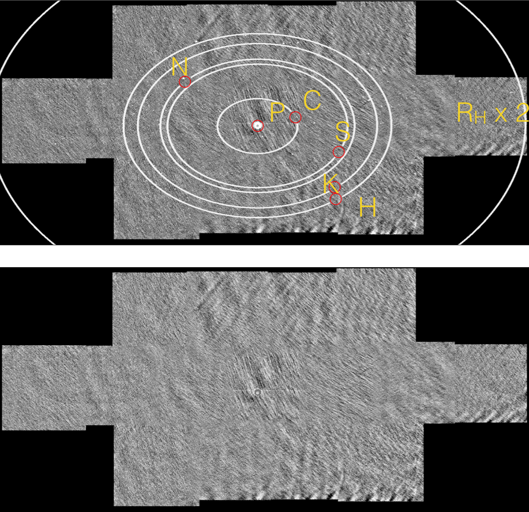
Figure 21: Top: LORRI mosaic O_RING_DEP_LORRI_202, overlain with orbits of Pluto’s satellites, with their positions marked (P=Pluto, and so forth). Bottom: Same, but with stars and Pluto-system bodies masked. The remaining structure is due to incompletely removed solar stray light.

For the day P$+7$ and P$+16$ sequences, $20\times 0.4$s exposures were obtained at each of the 15 positions, giving an 8s total exposure, although this is effectively doubled in the significant overlap areas (roughly $\sim 15\%$ of the field in both dimensions) between adjacent fields. On day P$+110$ the mosaic pattern was repeated 3 times, although with $15\times 0.4$s and $5\times 0.2$s exposures at each pointing for a total integration of $3\times(15\times 0.4+5\times 0.2)=21$s at any position (ignoring the overlap of adjacent fields).

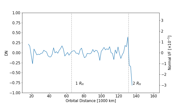
Figure 22: Radial profile from the O_RING_DEP_LORRI_202 mosaic.

As noted above, the LORRI mosaics were heavily compromised by the strong stray sunlight. The primary limitation is that the absolute intensity level of the stray light was a significant fraction of the CCD full well, requiring the exposures to be limited to only 0.4s, in contrast to the markedly deeper 10s exposures conducted during the hazard searches. Subtraction of the stray light was also problematic. The pattern of background light in any image was highly structured with features that changed rapidly with even small changes in spacecraft pointing with respect to the sun. We hoped that a PCA approach applied to the entire ensemble of LORRI search images could allow an accurate stray light model to be constructed for any given image, but unfortunately the behavior of the stray light had a component that was unique to any position, such that it could only be partially modeled by other images in the ensemble. PCA models did remove a portion of the stray light, but could not fully correct for it. Later analysis of the MVIC mosaics (see $\S\ref{sec:mvic}$) motivated a general-purpose algorithm for removing the ray-like streaks seen in some of the structure of the stray light, which did improve the reduction of the LORRI mosaics, but even perfect correction of the stray light would still leave behind the strong shot-noise associated with it.

We emphasize a strong caveat that was always kept in mind during the analysis of the forward-scattering mosaics was to not perform any reduction steps that would also eliminate real diffuse-features associated with dust rings or arcs. If, for example, one was only interested in compact point sources in the fields (although looking back at the system we presumed that any unknown minor satellites would be invisible), a high-pass spatial filter would quickly eliminate most of the stray light structure, but it would do so at the expense of any real well-resolved dust features also present. One could also attempt PCA on only the 20 (or 60 images for the day P$+110$ searches) at any position, but here the spacecraft pointing variations were relatively small, which again would mean that there would be little discrimination between real ring-features from the structure of the stray light.

6.3.2 Ring limits from the LORRI Observations

Despite these difficulties, we were able to produce reduced LORRI mosaics at each epoch that could be searched for forward-scattered light from any dust rings. We analyzed the outbound LORRI observations in much the same way as the MVIC observations. The mosaiced images were registered using field stars; we then created geometrical backplanes referenced to Pluto’s orbital plane, removed bright pixels, created radial profiles, and converted from DN to normal $I/F$. We used the calibration constant $\texttt{RSOLAR}=3.801\times 10^{5}{\rm DN/s}~{}({\rm erg~{}cm^{-2}~{}s^{-1}~{}\AA^{-1}~{}sr^{-1}})^{-1}$ for LORRI 4$\times$4 frames. An example image is shown in Figure 21, and the resulting radial profile in Figure 22.

Table 5: Measured MVIC and LORRI normal I/F limits.

	N=1000 radial bins		N=100 radial bins
	Resolution		Resolution
Sequence	(km)	Normal I/F	(km)	Normal I/F
O_RingDep_A_1 (MVIC)	136	$<5.0<\times 10^{-6}$	1,360	$<1.9\times 10^{-6}$
O_RING_DEP_MVICFRAME_202	432	$<2.1\times 10^{-6}$	4,320	$<1.1\times 10^{-6}$
O_RING_DEP_LORRI_202	159	$<2.8\times 10^{-5}$	1,590	$<1.4\times 10^{-5}$
O_RING_DEP_MVICFRAME_211	983	$<1.8\times 10^{-6}$	9,830	$<8.9\times 10^{-7}$
O_RING_DEP_LORRI_211		(not analyzed)
O_RING_DEP_MVICFRAME_305	6,814	$<1.5\times 10^{-6}$	68,140	$<7.3\times 10^{-7}$
O_RING_DEP_LORRI_305	2,834	$<1.3\times 10^{-4}$	28,340	$<1.2\times 10^{-4}$

We did not find any features suggestive of rings in the LORRI images or radial profile. Our lower limits are given in Table 5. The limits for LORRI are substantially worse (10-100$\times$) than those for MVIC, for two reasons. First, the LORRI exposures were much shorter, with the integrated time for longest observations 18s/pixel, vs. 750s for the MVIC observations at the same geometry. The stronger LORRI background, with the poorer corrections noted in the previous section, contribute the remaining lost of sensitivity. Because the LORRI mosaics were taken on the same dates as MVIC, but with shorter exposures and smaller fields, we did not create the mosaic and radial profiles for the remaining LORRI sequence O_RING_DEP_LORRI_211. The LORRI and MVIC observations were designed to be redundant, and the remaining LORRI data would not improve our $I/F$ limits.

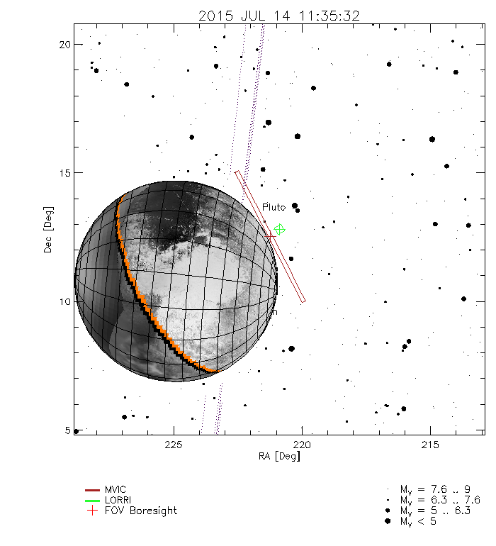
Figure 23: The geometry of the PEMV_01_P_MVIC_LORRI_CA MVIC scan is shown. The scan occured shortly before the spacecraft crossed Pluto’s equatorial plane. The field of MVIC is the narrow rectangle position off the limb of Pluto. During an MVIC scan the spacecraft is slowly rotated, and the field is scanned over the planet as the camera is read out using a time-delay integration mode. Dashed lines mark the orbits of the minor satellites, which traverse a small portion of the scan at only $\sim 3^{\circ}$ inclination.

7 Untargeted Ring Observations

The previous sections described the explicitly targeted ring-search observations. It is possible that rings or debris may be present and serendipitously detectable in other observations. In particular, NH passed through Pluto’s equatorial plane at approximately 2015, July 14 11:37:10 UT (spacecraft frame). Any ring material observed near this time would appear brightened substantially due to the high line-of-sight optical depth of a ring seen edge-on.

The equatorial crossing occurred approximately 11 minutes before the Pluto close-approach, so the cameras were observing Pluto’s surface at high resolution during this time. Due in part to uncertainty in Pluto’s position and the spacecraft’s pointing, some of the images recorded data off Pluto’s limb. None of the LORRI image fields passed directly through the (nearby) lit equatorial plane; however, the MVIC scan PEMV_01_P_MVIC_LORRI_CA obtained close to this time nominally includes a portion of the plane at very low inclination in the background off the limb of Pluto. The integration is short and the background is dominated by scattering from haze particles in Pluto’s atmosphere; no features associated with the orbits of the minor satellites were seen (Figure 23. We individually inspected all images around this time to search for any evidence of ring material, and didn’t find any. Because the line-of-sight did not directly intersect the expected ring plane, any material we did find would have been inclined. Since we cannot constrain the inclination or radial extent of these non-detections, we cannot use these to measure a meaningful upper limit.

8 Discussion and Summary

As Tables 1 and 2 show, substantial observational resources were dedicated to the task of searching for dust, debris, or rings within the Pluto-Charon system, using diverse tactics and instruments. The NH science team in turn devoted substantial effort to the reduction and analysis of these observations. Although no rings or dust clouds were found, the program did produce significantly improved upper limits on their allowed surface densities in the region of the small moons.

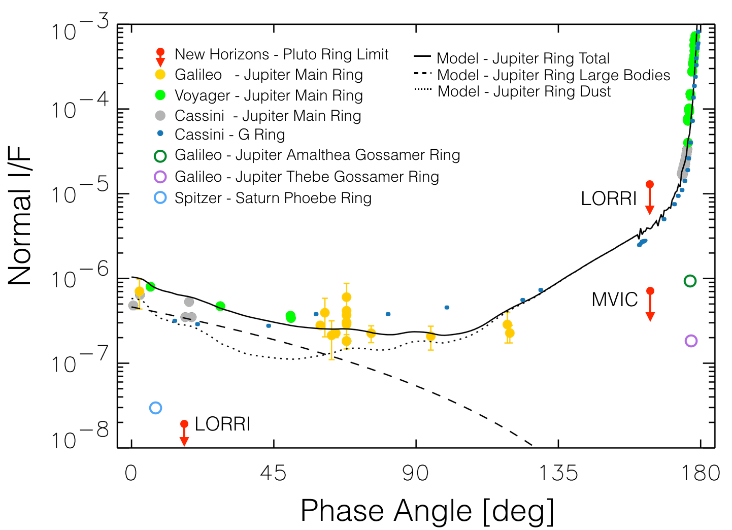
Figure 24: Comparison between New Horizons detection limits and brightness of several other rings. The $I/F$ (vertical axis) indicates relative reflectivity at each ring’s correct location. If Jupiter’s main ring was placed in orbit around Pluto, it would have been detectable on approach by LORRI, and on departure by MVIC, despite the much lower flux at Pluto. Saturn’s G ring would also have been detected by LORRI and MVIC. It is possible that NH could have barely detected the Phoebe and Amalthea rings, if they were in orbit around Pluto. On the other hand, Jupiter’s Thebe ring is too faint to be detected. Figure adapted from Throop et al. (2004). G ring data from Hedman & Stark (2015). Voyager, Cassini, and Galileo data, and model ring, from Throop et al. (2004) and references therein. Gossamer ring data from Ockert-Bell et al. (1999); Phoebe ring from Verbiscer et al. (2009).

In broad terms, NH provided superior resolution and sensitivity to search for back-scattered light from rings within the radial zone extending from the orbit of Styx, the innermost satellite, to twice the orbital radius of Hydra, the outermost satellite. The new HST observations provided the best constraints on broad features at large radii outside the satellite orbits.

At low phase angles, limits on the normal $I/F$ of narrow rings within this zone are $2\times 10^{-8}$ at the 1500 km resolution scale of the P$-64$ images, decreasing to $7\times 10^{-9}$ on $12,000$ km scales. We can convert these limits to optical depth $\tau$ via Eq. 1, assuming that the factor $A\times P(\alpha)/P(0)$ for rings is comparable to that for the small moons: $0.7\pm 0.2$ (Weaver et al., 2016). If this assumption is correct, then optical depth limits are $\sim 30$% larger than the normal $I/F$ limits.

New Horizons also provided the first high-phase vantage point to search for forward-scattered light from dust clouds or rings during its departure from Pluto over the entire Hill sphere. Here we derive limits of $\mu I/F<8.9\times 10^{-7}$ on $\sim 10^{4}$ km scales.

To aid in the interpretation of the these limits, we demonstrate in Figure 24 that we would have readily detected several of the diffuse rings around Jupiter or Saturn, had they been present at Pluto. Jupiter’s main ring would have been clearly seen, for example, despite the 40$\times$ lower solar flux at Pluto vs. Jupiter. Jupiter’s main ring has a normal $I/F\sim 5\times 10^{-6}$ and width $\sim 3000$ km (e.g., Throop et al., 2004). Significantly, it comprises a mix of rocky debris and fine dust, each component contributing a similar total cross-sectional area. Our MVIC mosaics would have readily detected the dust in the forward-scattering searches, at over an order of magnitude higher $I/F$ than our present limits, while the LORRI back-scattering searches would have detected the debris component, with again an order of magnitude sensitivity to spare. At the same time, the Gossamer ring associated with Jupiter’s satellite Thebe would have remained undetected. We cannot rule out the possibility that Pluto might still have rings similar to the most tenuous ones known to exist.

As outlined in the introduction, prior to the New Horizons, our expectations of whether Pluto could or even should, have rings remained unsettled. The discovery of four small satellites provided a clear source for dust debris generated by gardening. On the other hand, improved understanding of the role of solar radiation pressure in clearing such material from the system (Pires dos Santos et al., 2013), coupled with the complex and richly packed orbital dynamics of the satellite system (Youdin et al., 2012; Showalter & Hamilton, 2015) mitigate against the existence of long-lived rings.

Recently, Singer et al. (2017) found a marked paucity of small craters on Pluto and Charon in NH images. This would require a dearth of KBO impactors smaller than $\sim 1$ km in radius as compared to the pre-encounter assumed impactor-size distribution. In short, the smallest impactors appear to follow a markedly shallower distribution function, such that their integrated contribution to impact gardening may be decreased by well over an order of magnitude below that estimated by Durda & Stern (2000). This dearth of small-impactors is an additional stroke against detectable rings. The observational limits of the present work on the existence of dust or rings in the Pluto-Charon system offer an opportunity to revisit the theoretical expectations on the on-going production and removal of dust within the Kuiper Belt.

References

- Astropy Collaboration et al. (2013) Astropy Collaboration, Robitaille, T. P., Tollerud, E. J., et al. 2013, Astropy: A community Python package for astronomy. A&A, 558, A33
- Bagenal et al. (2016) Bagenal, F., Horányi, M., McComas, D. J., et al. 2016, Pluto’s interaction with its space environment: Solar wind, energetic particles, and dust. Science, 351, aad9045
- Bohlin et al. (2001) Bohlin, R. C., Dickinson, M. E., and Calzetti, D., 2011, Spectrophotometric standards from the far-ultraviolet to the near-infrared: STIS and NICMOS fluxes. AJ, 122, 2118–2128.
- Boissel et al. (2014) Boissel, Y., Sicardy, B., Roques, F., et al. 2014, An exploration of Pluto’s environment through stellar occultations. A&A, 561, A144
- Boroson & Lauer (2010) Boroson, T. A., & Lauer, T. R. 2010, Exploring the Spectral Space of Low Redshift QSOs. AJ, 140, 390
- Braga-Ribas et al. (2014) Braga-Ribas, F., Sicardy, B., Ortiz, J. L., et al. 2014, A ring system detected around the Centaur (10199) Chariklo. Nature, 508, 72
- Canup (2005) Canup, R. M. 2005, A Giant Impact Origin of Pluto-Charon. Science, 307, 546
- Cheng et al. (2008) Cheng, A. F., Weaver, H. A., Conard, S. J., et al. 2008, Long-Range Reconnaissance Imager on New Horizons. Space Sci. Rev., 140, 189
- Durda & Stern (2000) Durda, D. D., & Stern, S. A. 2000, Collision Rates in the Present-Day Kuiper Belt and Centaur Regions: Applications to Surface Activation and Modification on Comets, Kuiper Belt Objects, Centaurs, and Pluto-Charon. Icarus, 145, 220
- Giuliatti Winter et al. (2013) Giuliatti Winter, S. M., O. C. Winter, E. Vieira Neto, and R. Sfair, 2013, Stable regions around Pluto. Monthly Notices of the Royal Astronomical Society 430(3), 1892–1900.
- Hedman & Stark (2015) Hedman, M. M., & Stark, C. C. 2015, Saturn’s G and D Rings Provide Nearly Complete Measured Scattering Phase Functions of Nearby Debris Disks. ApJ, 811, 67
- Horányi et al. (2008) Horányi, M., Hoxie, V., James, D., et al. 2008, The Student Dust Counter on the New Horizons Mission. Space Sci. Rev., 140, 387
- Kenyon & Bromley (2014) Kenyon, S. J., & Bromley, B. C. 2014, The Formation of Pluto’s Low-mass Satellites. AJ, 147, 8
- Kammer et al. (2016) Kammer, J. A., Stern, S. A., Weaver, H. A., et al. 2016, Stargazing from New Horizons: Ultraviolet Stellar Occultations by Pluto’s Atmosphere. AAS/Division for Planetary Sciences Meeting Abstracts, 48, 306.02
- Krist et al. (2011) Krist J. E., Hook R. N., & Stoehr F. 2011, 20 years of Hubble Space Telescope optical modeling using Tiny Tim. Proc. of SPIE, 8127.
- Lang et al. (2010) Lang, D., Hogg, D. W., Mierle, K., Blanton, M., & Roweis, S. 2010, Astrometry.net: Blind Astrometric Calibration of Arbitrary Astronomical Images. AJ, 139, 1782
- Marton et al. (2015) Marton, G., Kiss, C., Balog, Z., et al. 2015, Search for signatures of dust in the Pluto-Charon system using Herschel/PACS observations. A&A, 579, L9
- McKinnon (1989) McKinnon, W. B. 1989, On the origin of the Pluto-Charon binary. ApJ, 344, L41
- Nimmo et al. (2017) Nimmo, F., Umurhan, O., Lisse, C. M., et al. 2017, Mean radius and shape of Pluto and Charon from New Horizons images Icarus, 287, 12
- Ockert-Bell et al. (1999) Ockert-Bell, M. E., Burns, J. A., Daubar, I. J., et al. 1999, The Structure of Jupiter’s Ring System as Revealed by the Galileo Imaging Experiment. Icarus, 138, 188
- Ortiz et al. (2015) Ortiz, J. L., Duffard, R., Pinilla-Alonso, N., et al. 2015, Possible ring material around centaur (2060) Chiron. A&A, 576, A18
- Pires dos Santos et al. (2013) Pires dos Santos, P. M., Giuliatti Winter, S. M., Sfair, R., & Mourão, D. C. 2013, Small particles in Pluto’s environment: effects of the solar radiation pressure. MNRAS, 430, 2761
- Poppe & Horányi (2011) Poppe, A., & Horányi, M. 2011, The effect of Nix and Hydra on the putative Pluto-Charon dust cloud. Planet. Space Sci., 59, 1647
- Porter & Grundy (2015) Porter, S. B., & Grundy, W. M. 2015, Ejecta transfer in the Pluto system. Icarus, 246, 360
- Porter & Stern (2015) Porter, S. B., & Stern, S. A. 2015, Orbits of Potential Pluto Satellites and Rings Between Charon and Hydra. arXiv:1505.05933
- Reuter et al. (2008) Reuter, D. C., Stern, S. A., Scherrer, J., et al. 2008, Ralph: A Visible/Infrared Imager for the New Horizons Pluto/Kuiper Belt Mission. Space Sci. Rev., 140, 129
- Ruprecht et al. (2015) Ruprecht, J. D., Bosh, A. S., Person, M. J., et al. 2015, 29 November 2011 stellar occultation by 2060 Chiron: Symmetric jet-like features. Icarus, 252, 271
- Seidelmann et al. (2007) Seidelmann, P. K., B. A. Archinal, M. F. A’Hearn, A. Conrad, G. J. Consolmagno, D. Hestroffer, J. L. Hilton, G. A. Krasinsky, G. Neumann, J. Oberst, P. Stooke, E. F. Tedesco, D. J. Tholen, P. C. Thomas, and I. P. Williams, 2007, Report of the IAU/IAG Working Group on cartographic coordinates and rotational elements: 2006. Celestial Mechanics and Dynamical Astronomy 98(3), 155–180.
- Showalter & Cuzzi (1993) Showalter, M. R., & Cuzzi J. N. 1993, Seeing ghosts: Photometry of Saturn’s G Ring. Icarus, 103, 124–143.
- Showalter et al. (2011) Showalter, M. R., Hamilton, D. P., Stern S. A., Weaver H. A., Steffl A. J., & Young L. A. 2011, New satellite of (134340) Pluto: S/2011 (134340) 1. IAU Circular 9221.
- Showalter et al. (2012) Showalter, M. R., Weaver H. A., Stern S. A., Steffl A. J., Buie, M. W., Merline W. J., Mutchler M. J., Soummer R., & Throop H. B. 2012, New satellite of (134340) Pluto: S/2012 (134340) 1. IAU Circular 9253.
- Showalter & Hamilton (2015) Showalter, M. R., and Hamilton, D. P., 2015, Resonant interactions and chaotic rotation of Pluto’s small moons. Nature, 522, 45–49.
- Sicardy et al. (2016) Sicardy, B., El Moutamid, M., Quillen, A. C., et al. 2016, Rings beyond the giant planets. arXiv:1612.03321
- Singer et al. (2017) Singer, K. N., et al. 2017, Impact craters on Pluto and Charon reveal a deficit of small Kuiper belt objects. Science, submitted
- Steffl & Stern (2007) Steffl, A. J., & Stern, S. A. 2007, First Constraints on Rings in the Pluto System. AJ, 133, 1485
- Stern (2009) Stern, S. A. 2009, Ejecta exchange and satellite color evolution in the Pluto system, with implications for KBOs and asteroids with satellites. Icarus, 199, 571
- Stern et al. (2006) Stern, S. A., Weaver, H. A., Steffl, A. J., et al. 2006, A giant impact origin for Pluto’s small moons and satellite multiplicity in the Kuiper belt. Nature, 439, 946
- Stern et al. (2008) Stern, S. A., D. C. Slater, J. Scherrer, J. Stone, G. Dirks, M. Versteeg, M. Davis, G. R. Gladstone, J. W. Parker, L. A. Young, and O. H. W. Siegmund, 2008, ALICE: The Ultraviolet Imaging Spectrograph Aboard the New Horizons Pluto-Kuiper Belt Mission. Space Science Reviews 140(1), 155–187.
- Stern et al. (2015) Stern, S. A., Bagenal, F., Ennico, K., et al. 2015, The Pluto system: Initial results from its exploration by New Horizons. Science, 350, aad1815
- Throop & Esposito (1998) Throop, H. B. and L. W. Esposito, 1998, G ring particle sizes derived from ring plane crossing observations. Icarus 131(1), 152–166.
- Throop et al. (2004) Throop, H. B., C. C. Porco, R. A. West, J. A. Burns, M. R. Showalter, and P. D. Nicholson, 2004, The Jovian rings: New results derived from Cassini, Galileo, Voyager, and Earth-based observations. Icarus 172, 59–77.
- Throop et al. (2009) Throop, H. B., Stern, S. A., Parker, J. W., Gladstone, G. R., & Weaver, H. A. 2009, Introducing GV : The Spacecraft Geometry Visualizer AAS/Division for Planetary Sciences Meeting Abstracts #41, 41, 68.20
- Throop et al. (2015) Throop, H. B., French, R. G., Shoemaker, K., et al. 2015, Limits on Pluto’s ring system from the June 12 2006 stellar occultation and implications for the New Horizons impact hazard. Icarus, 246, 345
- Verbiscer et al. (2009) Verbiscer, A. J., Skrutskie, M. F., & Hamilton, D. P. 2009, Saturn’s largest ring. Nature, 461, 1098
- Weaver et al. (2016) Weaver, H. A., Buie, M. W., Buratti, B. J., et al. 2016, The small satellites of Pluto as observed by New Horizons. Science, 351, aae0030
- Youdin et al. (2012) Youdin, A. N., Kratter, K. M., and Kenyon S. J. 2012, Circumbinary chaos: Using Pluto’s newest moon to constrain the masses of Nix and Hydra. ApJ, 755, 1–11.