An Incremental Slicing Method for Functional Programs

Abstract.

Several applications of slicing require a program to be sliced with respect to more than one slicing criterion. Program specialization, parallelization and cohesion measurement are examples of such applications. These applications can benefit from an incremental static slicing method in which a significant extent of the computations for slicing with respect to one criterion could be reused for another. In this paper, we consider the problem of incremental slicing of functional programs.

We first present a non-incremental version of the slicing algorithm which does a polyvariant analysis of functions. Since polyvariant analyses tend to be costly, we compute a compact context-independent summary of each function and then use this summary at the call sites of the function. The construction of the function summary is non-trivial and helps in the development of the incremental version. The incremental method on the other hand consists of a one-time pre-computation step that uses the non-incremental version to slice the program with respect to a fixed default slicing criterion and processes the results further to a canonical form. Presented with an actual slicing criterion, the incremental step involves a low-cost computation that uses the results of the pre-computation to obtain the slice.

We have implemented a prototype of the slicer for a pure subset of Scheme, with pairs and lists as the only algebraic data types. Our experiments show that the incremental step of the slicer runs orders of magnitude faster than the non-incremental version. We have also proved the correctness of our incremental algorithm with respect to the non-incremental version.

1. Introduction

Program slicing refers to the class of techniques that delete parts of a given program while preserving certain desired behaviors, for example, memory, state or parts of output. These behaviors are called slicing criteria. Applications of slicing include debugging (root-cause analysis), program specialization, parallelization and cohesion measurement. However, in some of the above applications, a program has to be sliced more than once, each time with a different slicing criterion. In such situations, the existing techniques (Weiser, 1984; Horwitz et al., ; Reps and Turnidge, 1996; Liu and Stoller, 2003; Rodrigues and Barbosa, 2006b; Silva et al., 2012) are inefficient as they typically analyze the program multiple times. Each round of analysis involves a fixed point computation on the program text or some intermediate form of the program, typically SDG in the case of imperative languages. We thus require an incremental approach to slicing which can avoid repeated fixpoint computation by reusing some of the information obtained while slicing the same program earlier with a different criterion.

($\mathbf{define}$ ($\mathbf{lcc}$ str lc cc)       ($\mathbf{if}$ ($\mathbf{null?}$ str)           ($\mathbf{return}$ ($\mathbf{cons}$ lc cc))           ($\mathbf{if}$ ($\mathbf{eq?}$ ($\mathbf{car}$ str) $nl$)               ($\mathbf{return}$ ($\mathbf{lcc}$ ($\mathbf{cdr}$ str)                                   (+ lc 1)                                   (+ cc 1)))               ($\mathbf{return}$ ($\mathbf{lcc}$ ($\mathbf{cdr}$ str)                                 $\pi_{1}$:lc                                 $\pi_{2}$:(+ cc 1)))))) $(\mbox{$\mathbf{define}$}\ (\mathbf{main})$       $(\mbox{$\mathbf{return}$}\ (\mathbf{lcc}\ \ldots\ 0~{}0))))$	($\mathbf{define}$ ($\mathbf{lcc}$ str lc $\square$)       ($\mathbf{if}$ ($\mathbf{null?}$ str)           ($\mathbf{return}$ ($\mathbf{cons}$ lc $\square$))           ($\mathbf{if}$ ($\mathbf{eq?}$ ($\mathbf{car}$ str) $nl$)               ($\mathbf{return}$ ($\mathbf{lcc}$ ($\mathbf{cdr}$ str)                                   (+ lc 1)                                    $\square$))               ($\mathbf{return}$ ($\mathbf{lcc}$ ($\mathbf{cdr}$ str)                                 $\pi_{1}$:lc                                 $\pi_{2}$: $\square$))))) $(\mbox{$\mathbf{define}$}\ (\mathbf{main})$       $(\mbox{$\mathbf{return}$}\ (\mathbf{lcc}\ \ldots\ 0~{}\square))))$	($\mathbf{define}$ ($\mathbf{lcc}$ str $\square$ cc)       ($\mathbf{if}$ ($\mathbf{null?}$ str)           ($\mathbf{return}$ ($\mathbf{cons}$ $\square$ cc))           ($\mathbf{if}$ ($\mathbf{eq?}$ ($\mathbf{car}$ str) $nl$)               ($\mathbf{return}$ ($\mathbf{lcc}$ ($\mathbf{cdr}$ str)                                   $\square$                                   (+ cc 1)))               ($\mathbf{return}$ ($\mathbf{lcc}$ ($\mathbf{cdr}$ str)                                 $\pi_{1}$: $\square$                                 $\pi_{2}$: (+ cc 1)))))) $(\mbox{$\mathbf{define}$}\ (\mathbf{main})$       $(\mbox{$\mathbf{return}$}\ (\mathbf{lcc}\ \ldots\ \square~{}0))))$
(a) Program to compute the number of lines and characters in a string.	(b) Slice of program in (a) to compute the number of lines only.	(c) Slice of program in (a) to compute the number of characters only.

Figure 1. A program in Scheme-like language and its slices. The parts that are sliced away are denoted by $\square$.

The example from (Reps and Turnidge, 1996) shown in Figure 1b motivates the need for incremental slicing. It shows a simple program in a Scheme-like language. It takes a string as input and returns a pair consisting of the number of characters and lines in the string. Figure 1b shows the program when it is sliced with respect to the first component of the output pair, namely the number of lines in the string (lc). All references to the count of characters (cc) and the expressions responsible for computing cc only have been sliced away (denoted $\square$). The same program can also be sliced to produce only the char count and the resulting program is shown in Figure 1c.

The example illustrates several important aspects for an effective slicing procedure. We need the ability to specify a rich set of slicing criteria to select different parts of a possibly complex output structure (first and second component of the output pair in the example, or say, every even element in an output list). Also notice that to compute some part of an output structure, all prefixes of the structure have to be computed. Thus, slicing criteria have to be prefix-closed. Finally, it seems likely from the example, that certain parts of the program will be present in any slice, irrespective of the specific slicing criterion. Thus, when multiple slices of the same program are required, a slicing procedure should strive for efficiency by minimizing re-computations related to the common parts.

In this paper, we consider the problem of incremental slicing for functional programs. We restrict ourselves to tuples and lists as the only algebraic data types. We represent our slicing criteria as regular grammars that represent sets of prefix-closed strings of the selectors $\mathbf{car}$ and $\mathbf{cdr}$. The slicing criterion represents the part of the output of the program in which we are interested, and we view it as being a demand on the program. We first present a non-incremental slicing method, which propagates the demand represented by the slicing criterion into the program. In this our method resembles the projection function based methods of (Reps and Turnidge, 1996; Liu and Stoller, 2003). However, unlike these methods, we do a context-sensitive analysis of functions calls. This makes our method precise by avoiding analysis over infeasible interprocedural paths. To avoid the inefficiency of analyzing a function once for each calling context, we create a compact context-independent summary for each function. This summary is then used to step over function calls. As we shall see, it is this context independent summary that also makes the incremental version possible in our approach.

The incremental version, has a one-time pre-computation step in which the program is sliced with respect to a default criterion that is same for all programs. The result of this step is converted to a set of automata, one for each expression in the program. This completes the pre-computation step. To decide whether a expression is in the slice for a given slicing criterion, we simply intersect the slicing criterion with the automaton corresponding to the expression. If the result is the empty set, the expression can be removed from the slice.

The main contributions of this paper are as follows:

1. We propose a view of the slicing criterion in terms of a notion called demand (Section 3) and formulate the problem of slicing as one of propagating the demand on the main expression to all the sub-expressions of the program. The analysis for this is precise because it keeps the information at the calling context separate. However it attempts to reduce the attendant inefficiency through the use of function summaries. The difficulty of creating function summaries in a polyvariant analysis, especially when the domain of analysis is unbounded, has been pointed out in (Reps and Turnidge, 1996).

2. Our formulation (Section 4) allows us to derive an incremental version of slicing algorithm that factors out computations common to all slicing criteria (Section 5) and re-uses these computations. To the best of our knowledge, the incremental version of slicing in this form has not been attempted before.

3. We have proven the correctness of the incremental slicing algorithm with respect to the non-incremental version (Section 5.2).

4. We have implemented a prototype slicer for a first-order version of Scheme (Section 7). We have also extended the implementation to higher-order programs (Section 6) by converting such programs to first-order using firstification techniques (Mitchell and Runciman, 2009), slicing the firstified programs using our slicer, and then mapping the sliced program back to the higher-order version. The implementation demonstrates the expected benefits of incremental slicing: the incremental step is one to four orders of magnitude faster than the non-incremental version.

$\begin{array}[]{@{}r@{\ }c@{\ }l@{}}p\in\mathit{Prog}&\!::=\!\!&d_{1}\ldots d_{n}\,\,e_{\mathbf{main}}\hskip 55.00008pt\mbox{\em--- program}\\ &\\ d\in\mathit{Fdef}&\!::=\!\!&(\mbox{$\mathbf{define}$}\,\,(f\,\,x_{1}\,\,\ldots\,\,x_{n})\,\,e)\hskip 15.00002pt\mbox{\em--- function definition}\\ &\\ e\in\mathit{Expr}&\!::=\!\!&\left\{\begin{array}[]{@{}ll@{\hspace{3.6em}}l}(\mbox{$\mathbf{if}$}\,\,x\,\,e_{1}\,\,e_{2})&\hfil\hskip 36.0001pt&\mbox{\em--- conditional}\\ (\mbox{$\mathbf{let}$}\,\,x\leftarrow s\,\,\mbox{$\mathbf{in}$}\,\,e)&\hfil\hskip 36.0001pt&\mbox{\em--- let binding}\\ (\mbox{$\mathbf{return}$}\,\,x)&\hfil\hskip 36.0001pt&\mbox{\em--- return from function}\end{array}\right.\\ &\\ s\in\mathit{App}&\!::=\!\!&\left\{\begin{array}[]{@{}l@{}r@{\hspace{1em}}l}k&$\mbox{$\mathbf{nil}$}$\hskip 10.00002pt&\mbox{\em--- constants}\\ (\mbox{$\mathbf{cons}$}\,\,x_{1}\,\,x_{2})&\hskip 10.00002pt&\mbox{\em--- constructor}\\ (\mbox{$\mathbf{car}$}\,\,x)&(\mbox{$\mathbf{cdr}$}\,\,x)\hskip 10.00002pt&\mbox{\em--- selectors}\\ (\mbox{$\mathbf{null?}$}\,\,x)&(\mbox{$\mathbf{+}$}\,\,x_{1}\,\,x_{2})\hskip 10.00002pt&\mbox{\em--- tester/generic-arithmetic}\\ \lx@intercol(f\,\,x_{1}\,\,\ldots\,\,x_{n})\hfil\lx@intercol&\mbox{\em--- function application}\end{array}\right.\\ \end{array}$

Figure 2. The syntax of our language

2. The target language—syntax and semantics

Figure 2 shows the syntax of our language. For ease of presentation, we restrict the language to Administrative Normal Form (ANF) (Chakravarty et al., 2003). In this form, the arguments to functions can only be variables. To avoid dealing with scope-shadowing, we assume that all variables in a program are distinct. Neither of these two restrictions affect the expressibility of our language. In fact, it is a simple matter to transform the pure subset of first order Scheme to our language, and map the sliced program back to Scheme. To refer to an expression $e$, we may annotate it with a label $\pi$ as $\pi\!:\!e$; however the label is not part of the language. To keep the description simple, we shall assume that each program has its own unique set of labels. In other words, a label identifies both the program point and the program that contains it.

A program in our language is a collection of function definitions followed by a main expression denoted as $e_{\mathbf{main}}$. Applications (denoted by the syntactic category $\mathit{App}$) consist of functions or operators applied to variables. Expressions ($\mathit{Expr}$) are either an $\mathbf{if}$ expression, a $\mathbf{let}$ expression that evaluates an application and binds the result to a variable, or a $\mathbf{return}$ expression. The $\mathbf{return}$ keyword is used to mark the end of a function so as to initiate appropriate semantic actions during execution. The distinction between expressions and applications will become important while specifying the semantics of programs.

$$\begin{array}[]{|@{\ }c@{\ }|c|c|}\hline\cr\mbox{Premise}&\mbox{Transition}&\mbox{Rule Name}\\ \hline\cr\hline\cr&\rho,\mathbf{H},k\rightsquigarrow\mathbf{H},k&\mbox{\sc const}\\ \hline\cr\rho(x)\in\mathbb{N}\quad\quad\rho(y)\in\mathbb{N}&\rho,\mathbf{H},(\mbox{$\mathbf{+}$}\,\,x\ y)\rightsquigarrow\mathbf{H},\rho(x)+\rho(y)&\mbox{\sc prim}\\ \hline\cr\mathbf{H}(\rho(x))=(v_{1},v_{2})&\rho,\mathbf{H},(\mbox{$\mathbf{car}$}\,\,x)\rightsquigarrow\mathbf{H},v_{1}&\mbox{\sc car}\\ \hline\cr\mathbf{H}(\rho(x))=(v_{1},v_{2})&\rho,\mathbf{H},(\mbox{$\mathbf{cdr}$}\,\,x)\rightsquigarrow\mathbf{H},v_{2}&\mbox{\sc cdr}\\ \hline\cr\mbox{$\ell\not\in\mbox{dom}(\mathbf{H})$ is a fresh location}&\rho,\mathbf{H},(\mbox{$\mathbf{cons}$}\,\,x\ y)\rightsquigarrow\mathbf{H}[\ell\mapsto(\rho(x),\rho(y))],\ell&\mbox{\sc cons}\\ \hline\cr\rho(x)\in\mathbb{N}\setminus\{0\}&\rho,\mathbf{S},\mathbf{H},(\mbox{$\mathbf{if}$}\ x\ e_{1}\ e_{2})\longrightarrow\rho,\mathbf{S},\mathbf{H},e_{1}&\mbox{\sc if-true}\\ \hline\cr\rho(x)=0&\rho,\mathbf{S},\mathbf{H},(\mbox{$\mathbf{if}$}\ x\ e_{1}\ e_{2})\longrightarrow\rho,\mathbf{S},\mathbf{H},e_{2}&\mbox{\sc if-false}\\ \hline\cr\rho(x)\not=\mbox{$\mathbf{nil}$}&\rho,\mathbf{H},(\mbox{$\mathbf{null?}$}\,\,x)\rightsquigarrow\mathbf{H},0&\mbox{\sc null-true}\\ \hline\cr\rho(x)=\mbox{$\mathbf{nil}$}&\rho,\mathbf{H},(\mbox{$\mathbf{null?}$}\,\,x)\rightsquigarrow\mathbf{H},1&\mbox{\sc null-false}\\ \hline\cr\begin{array}[]{@{\ }l@{\ }}\mbox{$s$ is $(f\,\,y_{1}\ldots y_{n})$}\\ \mbox{$f$ is $(\mbox{$\mathbf{define}$}\ (f\ z_{1}\ \ldots\ z_{n})\ e_{f})$}\end{array}&\rho,\mathbf{S},\mathbf{H},(\mbox{$\mathbf{let}$}\,\,x\leftarrow s\,\,\mbox{$\mathbf{in}$}\,\,e)\longrightarrow[\mathaccent 382{z}\mapsto\rho(\mathaccent 382{y})],\,(\rho,x,e)\bullet\mathbf{S},\,\mathbf{H},e_{f}&\mbox{\sc let-fncall}\\ \hline\cr\begin{array}[]{@{\ }l@{\ }}\rho,\mathbf{H},s\rightsquigarrow\mathbf{H}^{\prime},v\\ \mbox{$s$ is not $(f\,\,y_{1}\ldots y_{n})$ }\end{array}&\rho,\mathbf{S},\mathbf{H},(\mbox{$\mathbf{let}$}\,\,x\leftarrow s\,\,\mbox{$\mathbf{in}$}\,\,e)\longrightarrow\rho[x\mapsto v],\mathbf{S},\mathbf{H}^{\prime},e&\mbox{\sc let-nonfn}\\ \hline\cr&\rho,\,(\rho^{\prime},x^{\prime},e^{\prime})\bullet\mathbf{S},\,\mathbf{H},(\mbox{$\mathbf{return}$}\ x)\longrightarrow\rho^{\prime}[x^{\prime}\mapsto\rho(x)],\mathbf{S},\mathbf{H},e^{\prime}&\mbox{\sc return}\\ \hline\cr\end{array}$$

Figure 3. The semantics of our language

2.1. Semantics

We now present the operational semantics for our language. This is largely borrowed from (Asati et al., ; Kumar et al., 2016) and we include it here for completeness. We start with the domains used by the semantics:

$$\begin{array}[]{rlcl@{\hspace{2em}}l}v:&\mathit{Val}&=&\mathbb{N}+\{\mbox{$\mathbf{nil}$}\}+\mathit{Loc}\hfil\hskip 20.00003pt&\mbox{-- Values}\\ \rho:&\mathit{Env}&=&\mathit{Var}\rightarrow{Val}\hfil\hskip 20.00003pt&\mbox{-- Environment}\\ \mathbf{H}:&\mathit{Heap}&=&\mathit{Loc}\rightarrow(Val\times Val+\{empty\})\hfil\hskip 20.00003pt&\mbox{-- Heap}\end{array}$$

A value in our language is either a number, or the empty list denoted by $\mathbf{nil}$, or a location in the heap. The heap maps each location to a pair of values denoting a cons cell. Heap locations can also be empty. Finally, an environment is a mapping from variables to values.

The dynamic aspects of the semantics, shown in Figure 3, are specified as a state transition system. The semantics of applications $s$ are given by the judgement form $\rho,\mathbf{H},s\rightsquigarrow\mathbf{H}^{\prime},v$, and those for expressions $e$ by the form $\rho,\mathbf{S},\mathbf{H},e\rightarrow\rho^{\prime},\mathbf{S}^{\prime},\mathbf{H}^{\prime},e^{\prime}$. Here $\mathbf{S}$ is a stack consisting of continuation frames of the form $(\rho,x,e)$. The frame $(\rho,x,e)$ signifies that if the current function returns a value $v$, the next expression to be evaluated is $e$, and the environment for this evaluation is $\rho$ updated with the variable $x$ bound to $v$. The start state is $(\{\}_{\rho},[\,]_{\mathbf{S}},\{\}_{\mathbf{H}},e_{\mathbf{main}})$, where $\{\}_{\rho}$ is the empty environment, $[\,]_{\mathbf{S}}$ is the empty stack, and $\{\}_{\mathbf{H}}$ is the empty heap. The program terminates successfully with result value $\rho(x)$ on reaching the halt state $(\rho,[\,]_{\mathbf{S}},\mathbf{H},(\mbox{$\mathbf{return}$}\ x))$. We use the notation $\rho[x\mapsto v]$ to denote the environment obtained by updating $\rho$ with the value for $x$ as $v$. We also use $[\mathaccent 382{x}\mapsto\mathaccent 382{v}]$ to denote an environment in which each $x_{i}$ has the value $v_{i}$.

3. Demand

We now connect slicing with a notion called demand. A demand on an expression represents the set of paths that the context of the expression may explore of the value of the expression. A demand is represented by a prefix-closed set of strings over $(\mathbf{0}+\mathbf{1})^{\ast}$. Each string in the demand, called an access path, represents a traversal over the heap. $\mathbf{0}$ stands for a single-step traversal over the heap by dereferencing the $\mathbf{car}$ field of a cons cell. Similarly, $\mathbf{1}$ denotes the dereferencing of the $\mathbf{cdr}$ field of a cons cell.

As an example, a demand of $\{\epsilon,\mathbf{1},\mathbf{1}\mathbf{0}\}$ on the expression $(\mbox{$\mathbf{cons}$}~{}x~{}y)$ means its context may need to visit the $\mathbf{car}$ field of $y$ in the heap (corresponding to the string $\mathbf{1}$$\mathbf{0}$ in the demand). The example also illustrates why demands are prefix-closed—the $\mathbf{car}$  field of $y$ cannot be visited without visiting first the cons cell resulting from the evaluation of $(\mbox{$\mathbf{cons}$}~{}x~{}y)$ (represented by $\epsilon$) and then the cell corresponding to $y$ (represented by $\mathbf{1}$). The absence of $\mathbf{0}$ in the demand also indicates that $x$ is definitely not visited. Notice that to meet the demand $\{\epsilon,\mathbf{1},\mathbf{1}\mathbf{0}\}$ on $(\mbox{$\mathbf{cons}$}~{}x~{}y)$, the access paths $\{\epsilon,\mathbf{0}\}$ has to be visited starting from $y$. Thus we can think of $(\mbox{$\mathbf{cons}$}~{}x~{}y)$ as a demand transformer transforming the demand $\{\epsilon,\mathbf{1},\mathbf{1}\mathbf{0}\}$ to the demand $\{\epsilon,\mathbf{0}\}$ on $y$ and the empty demand (represented by $\emptyset$) on $x$.

The slicing problem is now modeled as follows. Viewing the slicing criterion (also a set of strings over $(\mathbf{0}+\mathbf{1})^{\ast}$) as a demand on the main expression $e_{\mathbf{main}}$, we compute the demand on each expression in the program. If the demand on a expression turns out to be $\emptyset$, the expression does not contribute to the demand on $e_{\mathbf{main}}$ and can be removed from the slice. Thus the solution of the slicing problem lies in computing a demand transformer that, given a demand on $e_{\mathbf{main}}$, computes a demand environment—a mapping of each expression (represented by its program point $\pi$) to its demand. We formulate this computation as an analysis called demand analysis.

We use $\sigma$ to represent demands and $\alpha$ to represent access path. Given two access paths $\alpha_{1}$ and $\alpha_{2}$, we use the juxtaposition $\alpha_{1}\alpha_{2}$ to denote their concatenation. We extend this notation to a concatenate a pair of demands and even to the concatenation of a symbol with a demand: $\sigma_{1}\sigma_{2}$ denotes the demand $\{\alpha_{1}\alpha_{2}\mid\alpha_{1}\in\sigma~{}\mbox{and}~{}\alpha_{2}\in\sigma_{2}\}$ and $\mathbf{0}\sigma$ is a shorthand for $\{\mathbf{0}\alpha\mid\alpha\in\sigma\}$.

$$\mathit{\mathcal{A}}(\pi\!\!:\!\!\kappa,\sigma,\mathds{DS}) =\{\pi\mapsto\sigma\},\ \text{for constants including}\ \mathbf{nil}$$

$$\mathit{\mathcal{A}}(\pi\!\!:\!\!(\mathbf{null?}\ \pi_{1}\!\!:\!\!x),\sigma,\mathds{DS}) =\{\pi_{1}\mapsto\mbox{if}~{}\sigma\neq\emptyset~{}\mbox{then}~{}\{\epsilon\}~{}\mbox{else}~{}\emptyset,\;\pi\mapsto\sigma\}$$

$$\mathit{\mathcal{A}}(\pi\!\!\!:\!\!(\mbox{$\mathbf{+}$}\ \pi_{1}\!\!:\!\!x\ \pi_{2}\!\!:\!\!y),\sigma,\mathds{DS}) =\{\pi_{1}\mapsto\mbox{if}~{}\sigma\neq\emptyset~{}\mbox{then}~{}\{\epsilon\}~{}\mbox{else}~{}\emptyset,\;\;\pi_{2}\mapsto\mbox{if}~{}\sigma\neq\emptyset~{}\mbox{then}~{}\{\epsilon\}~{}\mbox{else}~{}\emptyset,\;\;\pi\mapsto\sigma\}$$

$$\mathit{\mathcal{A}}(\pi\!\!:\!\!:(\mathbf{car}\;\pi_{1}\!\!:x),\sigma,\mathds{DS}) =\{\pi_{1}\mapsto\mbox{if}~{}\sigma\neq\emptyset~{}\mbox{then}~{}\{\epsilon\}\cup\mathbf{0}\sigma~{}\mbox{else}~{}\emptyset,\;\;\pi\mapsto\sigma\}$$

$$\mathit{\mathcal{A}}(\pi\!\!:\!\!:(\mathbf{cdr}\;\pi_{1}\!\!:x),\sigma,\mathds{DS}) =\{\pi_{1}\mapsto\mbox{if}~{}\sigma\neq\emptyset~{}\mbox{then}~{}\{\epsilon\}\cup\mathbf{1}\sigma~{}\mbox{else}~{}\emptyset,\;\;\pi\mapsto\sigma\}$$

$$\mathit{\mathcal{A}}(\pi\!\!:\!\!(\mathbf{cons}\ \pi_{1}\!\!:\!\!x\ \pi_{2}\!\!:\!\!y),\sigma,\mathds{DS}) =\{\pi_{1}\!\mapsto\{\alpha\mid\mathbf{0}\alpha\in\sigma\},\pi_{2}\!\mapsto\{\alpha\mid\mathbf{1}\alpha\in\sigma\},\;\;\pi\mapsto\sigma\}$$

$$\mathit{\mathcal{A}}(\pi\!\!:\!\!(f\ \pi_{1}\!\!:\!\!y_{1}\ \cdots\ \pi_{n}\!\!:\!\!y_{n}),\sigma,\mathds{DS}) =\bigcup_{i=1}^{n}\{\pi_{i}\mapsto\mathds{DS}^{i}_{f}(\sigma)\}\cup\{\pi\mapsto\sigma\}$$

$$\mathcal{D}(\pi\!\!:\!\!(\mathbf{return}\ \pi_{1}\!\!:\!\!x),\sigma,\mathds{DS}) =\{\pi_{1}\mapsto\sigma,\pi\mapsto\sigma\}$$

$$\mathcal{D}(\pi\!\!:\!\!(\mathbf{if}\ \pi_{1}\!\!:\!\!x~{}e_{1}~{}e_{2}),\sigma,\mathds{DS}) =\mathcal{D}(e_{1},\sigma,\mathds{DS})\cup\mathcal{D}(e_{2},\sigma,\mathds{DS})~{}\cup\;\{\pi_{1}\mapsto\mbox{if}~{}\sigma\neq\emptyset~{}\mbox{then}~{}\{\epsilon\}~{}\mbox{else}~{}\emptyset,\;\pi\mapsto\sigma\}$$

$$\mathcal{D}(\pi\!\!:\!\!(\mathbf{let}\ \pi_{1}\!\!:\!\!x\leftarrow s\ \mathbf{in}\ e),\sigma,\mathds{DS}) ={\mathcal{A}}(s,\mathop{\cup}_{\pi\in\Pi}\mbox{DE}(\pi),\mathds{DS})\;\cup\{\pi\mapsto\sigma\}$$

$$~{}~{}~{}~{}\text{where}\ \mbox{DE}=\mathcal{D}(e,\sigma,\mathds{DS}),~{}\text{and}~{}~{}\Pi~{}\text{represents all occurrences of $x$ in $e$},$$

$\displaystyle\frac{\begin{array}[]{@{}c@{}}\forall f,\forall i,\forall\sigma:\;\;\mathcal{D}(e_{\mathit{f}},\sigma,\mathds{DS})=\mbox{DE},\mathds{DS}^{i}_{\mathit{f}}=\mathop{\bigcup}_{\pi\in\Pi}~{}\mbox{DE}(\pi)\end{array}}{\begin{array}[]{@{}c@{}}\mathit{df_{1}}\ldots\mathit{df_{k}}\ \vdash^{l}\ \mathds{DS}\end{array}}$ (demand-summary)

where $(\mbox{$\mathbf{define}$}\ (f\ z_{1}\ \ldots\ z_{n})\ \ e_{\mathit{f}})$ is one of $\mathit{df_{1}}$ …$\mathit{df_{k}}$, $1\leq i\leq n$, and $\Pi$ represents all occurrences of $z_{i}$ in $e_{f}$

Figure 4. Demand Analysis

3.1. Demand Analysis

Figure 4 shows the analysis. Given an application $s$ and a demand $\sigma$, $\mathcal{A}$  returns a demand environment that maps expressions of $s$ to their demands. The third parameter to $\mathcal{A}$, denoted $\mathds{DS}$, represents context-independent summaries of the functions in the program, and will be explained shortly.

Consider the rule for the selector $\mathbf{car}$. If the demand $\sigma$ on $(\mbox{$\mathbf{car}$}~{}x)$ is $\emptyset$, then no part of the value of $(\mbox{$\mathbf{car}$}~{}x)$ is visited and the demand on $x$ is also $\emptyset$. However, if $\sigma$ is non-empty, the context of $(\mbox{$\mathbf{car}$}~{}x)$ has to first dereference the value of $x$ using the $\mathbf{car}$ field and then traverse the paths represented by $\sigma$. In this case, the demand on $x$ is the set consisting of $\epsilon$ (start at the root of $x$) and $\mathbf{0}\sigma$ (dereference using $\mathbf{car}$  and then visit the paths in $\sigma$). On the other hand, the rule for the constructor $\mathbf{cons}$  works as follows: To traverse the path $\mathbf{0}\alpha$ (alternately $\mathbf{1}\alpha$) starting from the root of $(\mbox{$\mathbf{cons}$}~{}x~{}y)$, one has to traverse the path $\alpha$ starting from $x$ (or $y$).

Since $(\mathbf{null?}~{}x)$ only visits the root of $x$ to examine the constructor, a non-null demand on $(\mathbf{null?}~{}x)$ translates to the demand $\epsilon$ on $x$. A similar reasoning also explains the rule for $(\mbox{$\mathbf{+}$}~{}x~{}y)$. Since, both $x$ and $y$ evaluate to integers in a well typed program, a non-null demand on $(\mbox{$\mathbf{+}$}~{}x~{}y)$ translates to the demand $\epsilon$ on both $x$ and $y$.

The rule for a function call uses a third parameter $\mathds{DS}$ that represents the summaries of all functions in the program. $\mathds{DS}$ is a set of context-independent summaries, one for each (function, parameter) pair in the program. $\mathds{DS}_{\mathit{f}}^{\mathit{i}}$ represents a transformation that describes how any demand $\sigma$ on a call to $f$ is transformed into the demand on its $i$th parameter. $\mathds{DS}$ is specified by the inference rule demand-summary. This rule gives a fixed-point property to be satisfied by $\mathds{DS}$, namely, the demand transformation assumed for each function in the program should be the same as the demand transformation calculated from the body of the function. Given $\mathds{DS}$, the rule for the function call is obvious. Notice that the demand environment for each application $s$ also includes the demand on $s$ itself apart from its sub-expressions. Operationally, the rule demand-summary is converted into a grammar (Section 4) that is parameterized with respect to a placeholder terminal representing a symbolic demand. The language generated by this grammar is the least solution satisfying the rule. The least solution corresponds to the most precise slice.

We finally discuss the rules for expressions given by $\mathcal{D}$. The rules for $\mathbf{return}$ and $\mathbf{if}$  are obvious. The rule for $(\mathbf{let}\ x\leftarrow s\ \mathbf{in}\ e)$ first uses $\sigma$ to calculate the demand environment DE of the $\mathbf{let}$-body $e$. The demand on $s$ is the union of the demands on all occurrences of $x$ in $e$. It is easy to see by examining the rules that the analysis results in demands that are prefix-closed. More formally, let $\mbox{DE}_{\sigma}$ be the demand environment resulting from the analysis of a program for a demand $\sigma$. Then, for an expression $\pi\!\!:\!e$ in the program, $\mbox{DE}_{\sigma}(\pi)$ is prefix closed.

4. Computing Context-Independent Function Summaries

A slicing method used for, say, debugging needs to be as precise as possible to avoid false errors. We therefore choose to analyze each function call separately with respect to its calling context. We now show how to obtain a context-independent summary for each function definition from the rule demand-summary. Recall that this summary is a function that transforms any demand on the result of a call to demands on the arguments. A convenient way of doing this is to express how a symbolic demand is transformed by the body of a function. Summarizing the function in this way has two benefits. It helps us to propagate a demand across several calls to a function without analyzing its body each time. Even more importantly, it is the key to our incremental slicing method.

However, notice that the rules of demand analysis requires us to do operations that cannot be done on a symbolic demand. The $\mathbf{cons}$ rule, for example is defined in terms of the set $\{\alpha\mid\mathbf{0}\alpha\in\sigma\}$. Clearly this requires us to know the strings in $\sigma$. Similarly, the $\mathbf{if}$ rule requires to know whether $\sigma$ is $\emptyset$. The way out is to treat these operations also symbolically. For this we introduce three new symbols $\bar{}\mathbf{0}$, $\bar{}\mathbf{1}$ and ${\mathbf{2}}$, to capture the intended operations. If $\mathbf{0}$ represents selection using $\mathbf{car}$, $\bar{}\mathbf{0}$ is intended to represent a use as the left argument of $\mathbf{cons}$. Thus $\bar{}\mathbf{0}$$\mathbf{0}$ should reduce to the empty string $\epsilon$. Similarly ${\mathbf{2}}$ represents the symbolic transformation of any non-null demand to $\epsilon$ and null demand to itself. These transformation are defined and also made deterministic through the simplification function $\mathcal{S}$.

$$\mathcal{S}(\{\epsilon\}) =\{\epsilon\}$$

$$\mathcal{S}(\mathbf{0}\sigma) =\mathbf{0}\mathcal{S}(\sigma)$$

$$\mathcal{S}(\mathbf{1}\sigma) =\mathbf{1}\mathcal{S}(\sigma)$$

$$\mathcal{S}(\bar{}\mathbf{0}\sigma) =\{\alpha\mid\mathbf{0}\alpha\in\mathcal{S}(\sigma)\}$$

$$\mathcal{S}(\bar{}\mathbf{1}\sigma) =\{\alpha\mid\mathbf{1}\alpha\in\mathcal{S}(\sigma)\}$$

$$\mathcal{S}({\mathbf{2}}\sigma) =\left\{\begin{array}[]{ll}\emptyset&\mbox{if}~{}\mathcal{S}(\sigma)=\emptyset\\ \{\epsilon\}&\mbox{otherwise}\end{array}\right.$$

$$\mathcal{S}(\sigma_{1}\cup\sigma_{2}) =\mathcal{S}(\sigma_{1})\cup\mathcal{S}(\sigma_{2})$$

Notice that $\bar{}\mathbf{0}$  strips the leading $\mathbf{0}$ from the string following it, as required by the rule for $\mathbf{cons}$. Similarly, ${\mathbf{2}}$ examines the string following it and replaces it by $\emptyset$ or $\{\epsilon\}$; this is required by several rules. The $\mathcal{A}$ rules for $\mathbf{cons}$ and $\mathbf{car}$ in terms of the new symbols are:

$$\mathcal{A}(\pi\!\!:\!(\mbox{$\mathbf{cons}$}~{}\pi_{1}\!\!:\!x~{}\pi_{2}\!\!:\!y),\sigma,\mathds{DS})=\{\pi_{1}\mapsto\bar{}\mathbf{0}\sigma,\pi_{2}\mapsto\bar{}\mathbf{1}\sigma,\pi\mapsto\sigma\}~{}$$

$$\mathcal{A}(\pi\!\!:\!(\mbox{$\mathbf{car}$}~{}\pi_{1}\!\!:\!x),\sigma,\mathds{DS})=\{\pi_{1}\mapsto{\mathbf{2}}\sigma\cup\mathbf{0}\sigma,\pi\mapsto\sigma\}$$

and the $\mathcal{D}$ rule for $\mathbf{if}$ is:

$$\mathcal{D}(\pi\!\!:\!(\mbox{$\mathbf{if}$}~{}\pi_{1}\!\!:\!x~{}e_{1}~{}e_{2}),\sigma,\mathds{DS}) =\mathcal{D}(e_{1},\sigma,\mathds{DS})\cup\mathcal{D}(e_{2},\sigma,\mathds{DS})~{}\cup$$

$$~{}~{}~{}~{}\{\pi_{1}\mapsto\mbox{if}~{}\sigma\neq\emptyset~{}\mbox{then}~{}\{\epsilon\}~{}\mbox{else}~{}\emptyset,$$

$$~{}~{}~{}~{}\pi\mapsto\sigma\}$$

The rules for $\mathbf{cdr}$, $\mathbf{+}$  and $\mathbf{null?}$  are also modified similarly. Now the demand summaries can be obtained symbolically with the new symbols as markers indicating the operations that should be performed string following it. When the final demand environments are obtained with the given slicing criterion acting a concrete demand for the main expression $e_{\mathbf{main}}$, the symbols $\bar{}\mathbf{0}$, $\bar{}\mathbf{1}$  and ${\mathbf{2}}$  are eliminated using the simplification function $\mathcal{S}$.

4.1. Finding closed-forms for the summaries $\mathds{DS}$

Recall that $\mathds{DS}_{f}^{i}$ is a function that describes how the demand on a call to $f$ translates to its $i$th argument. A straightforward translation of the demand-summary rule to obtain $\mathds{DS}_{f}^{i}$ is as follows: For a symbolic demand $\sigma$ compute the the demand environment in $e_{f}$, the body of $f$. From this calculate the demand on the $i$th argument of $f$, say $x$. This is the union of demands of all occurrences of $x$ in the body of $f$. The demand on the $i$th argument is equated to $\mathds{DS}_{f}^{i}(\sigma)$. Since the body may contain other calls, the demand analysis within $e_{f}$ makes use of $\mathds{DS}$ in turn. Thus our equations may be recursive. On the whole, $\mathds{DS}$ corresponds to a set of equations, one for each argument of each function. The reader can verify that $\mathds{DS}_{\mathit{\mathbf{lcc}}}^{2}({\mathit{\sigma}})$ in our running example is:

$$\mathds{DS}_{\mathit{\mathbf{lcc}}}^{2}({\mathit{\sigma}}) = \bar{}\mathbf{0}\sigma\cup{\mathbf{2}}\mathds{DS}_{\mathit{\mathbf{lcc}}}^{2}({\mathit{\sigma}})$$

As noted in (Reps and Turnidge, 1996), the main difficulty in obtaining a convenient function summary is to find a closed-form description of $\mathds{DS}_{\mathit{\mathbf{lcc}}}^{2}({\mathit{\sigma}})$ instead of the recursive specification. Our solution to the problem lies in the following observation: Since we know that the demand rules always prefix symbols to the argument demand $\sigma$, we can write $\mathds{DS}_{\mathit{f}}^{i}({\mathit{\sigma}})$ as $\mathsf{DS}_{\mathit{f}}^{i}\sigma$, where $\mathsf{DS}_{\mathit{f}}^{i}$ is a set of strings over the alphabet $\{\mathbf{0},\mathbf{1},\bar{}\mathbf{0},\bar{}\mathbf{1},{\mathbf{2}}\}$. The modified equations after doing this substitution will be,

$$\mathsf{DS}_{\mathit{\mathbf{lcc}}}^{2}\sigma = \bar{}\mathbf{0}\sigma\cup{\mathbf{2}}\mbox{$\mathsf{DS}_{\mathit{\mathbf{lcc}}}^{2}\sigma$}$$

Thus, we have,

$$\mathds{DS}_{\mathit{\mathbf{lcc}}}^{2}({\mathit{\sigma}}) = \mathsf{DS}_{\mathit{\mathbf{lcc}}}^{2}\sigma$$

$$\mbox{where }\mathsf{DS}_{\mathit{\mathbf{lcc}}}^{2} = \{\bar{}\mathbf{0}\}\cup{\mathbf{2}}\mathsf{DS}_{\mathit{\mathbf{lcc}}}^{2}$$

4.2. Computing the demand environment for the function bodies

The demand environment for a function body $e_{\mathit{f}}$ is calculated with respect to a concrete demand. To start with, we consider the main expression $e_{\mathbf{main}}$ as being the body of a function $\mathbf{main}$, The demand on $e_{\mathbf{main}}$ is the given slicing criterion. Further, the concrete demand on a function $f$, denoted $\sigma_{f}$, is the union of the demands at all call-sites of $f$. The demand environment of a function body $e_{f}$ is calculated using $\sigma_{f}$. If there is a call to $g$ inside $e_{f}$, the demand summary $\mathds{DS}_{g}$ is used to propagate the demand across the call. Continuing with our example, the union of the demands on the three calls to $\mathbf{lcc}$ is the slicing criterion. Therefore the demand on the expression at program point $\pi_{1}$ is given by

(4) $$\begin{array}[]{rcl}\mathsf{D}_{\pi_{1}}&=&\mathsf{DS}_{\mathit{\mathbf{lcc}}}^{2}{\sigma_{\mathbf{lcc}}}\\ \mathsf{DS}_{\mathit{\mathbf{lcc}}}^{2}&=&\{\bar{}\mathbf{0}\}\cup{\mathbf{2}}\mathsf{DS}_{\mathit{\mathbf{lcc}}}^{2}\\ \sigma_{\mathbf{lcc}}&=&\mbox{slicing criterion}\end{array}$$

At the end of this step, we shall have (i) A set of equations defining the demand summaries $\mathds{DS}_{\mathit{f}}^{i}$ for each argument of each function, (ii) Equations specifying the demand $\mathsf{D}_{\pi}$ at each program point $\pi$, and (iii) an equation for each concrete demand $\sigma_{f}$ on the body of each function $f$.

4.3. Converting analysis equations to grammars

Notice that the equations for $\mathsf{DS}_{\mathit{\mathbf{lcc}}}^{2}$ are still recursive. However, Equation 4 can also be viewed as a grammar with $\{\mathbf{0},\mathbf{1},\bar{}\mathbf{1},\bar{}\mathbf{0},{\mathbf{2}}\}$ as terminal symbols and $\mathsf{DS}_{\mathit{\mathbf{lcc}}}^{2}$, $\mathsf{D}_{\pi_{1}}$ and $\sigma_{\mathbf{lcc}}$ as non-terminals. Thus finding the solution to the set of equations generated by the demand analysis reduces to finding the language generated by the corresponding grammar. The original equations can now be re-written as grammar rules as shown below:

(5) $$\begin{split}\raisebox{1.13809pt}{$\mathsf{D}_{\pi_{1}}$}&\rightarrow\raisebox{1.13809pt}{$\mathsf{DS}_{\mathit{\mathbf{lcc}}}^{2}$}\raisebox{1.13809pt}{$\sigma_{\mathbf{lcc}}$}\\ \raisebox{1.13809pt}{$\mathsf{DS}_{\mathit{\mathbf{lcc}}}^{2}$}&\rightarrow\bar{}\mathbf{0}\mid{\mathbf{2}}\;\raisebox{1.13809pt}{$\mathsf{DS}_{\mathit{\mathbf{lcc}}}^{2}$}\\ \raisebox{1.13809pt}{$\sigma_{\mathbf{lcc}}$}&\rightarrow\mbox{slicing criteria}\end{split}$$

Thus the question whether the expression at $\pi_{1}$ can be sliced for the slicing criterion $\sigma_{\mathbf{lcc}}$ is equivalent to asking whether the language $\mathcal{S}(\mathsf{L}({\mathsf{D}_{\pi_{1}}}))$ is empty. In fact, the simplification process $\mathcal{S}$ itself can be captured by adding the following set of five unrestricted productions named $\mathit{unrestricted}$ and adding the production $\raisebox{1.13809pt}{$\mathsf{D}^{\prime}_{\pi_{1}}$}\rightarrow\raisebox{1.13809pt}{$\mathsf{D}_{\pi_{1}}$}\$$ to the grammar generated earlier.

$$\bar{}\mathbf{0}\mathbf{0}\rightarrow\epsilon \bar{}\mathbf{1}\mathbf{1}\rightarrow\epsilon$$

$${\mathbf{2}}\$\rightarrow\epsilon {\mathbf{2}}\mathbf{0}\rightarrow{\mathbf{2}}$$

$${\mathbf{2}}\mathbf{1}\rightarrow{\mathbf{2}}$$

The set of five unrestricted productions shown are independent of the program being sliced and the slicing criterion. The symbol $ marks the end of a sentence and is required to capture the ${\mathbf{2}}$ rule correctly.

We now generalize: Assume that $\pi$ is the program point associated with an expression $e$. Given a slicing criterion $\sigma$, let $G_{\pi}^{\sigma}$ denote the grammar $(N,~{}T,~{}P_{\pi}^{\sigma}\cup\mathit{unrestricted}\cup\{\mathsf{D}^{\prime}_{\pi}\rightarrow\mathsf{D}_{\pi}\$\},~{}\raisebox{1.13809pt}{$\mathsf{D}^{\prime}_{\pi}$})$. Here $T$ is the set of terminals $\{\mathbf{0},\mathbf{1},\bar{}\mathbf{0},\bar{}\mathbf{1},{\mathbf{2}},\$\}$, $P_{\pi}^{\sigma}$ is the set of context-free productions defining $\mathsf{D}_{\pi}$, the demand on $e$ (as illustrated by example 5). $N$ contains the non-terminals of $P_{\pi}^{\sigma}$ and additionally includes the special non-terminal $\mathsf{D}^{\prime}_{\pi}$. As mentioned earlier, given a slicing criterion $\sigma$, the question of whether the expression $e$ can be sliced out of the containing program is equivalent to asking whether the language $\mathsf{L}({G_{\pi}^{\sigma}})$ is empty. We shall now show that this problem is undecidable.

Theorem 4.1.

Given a program point $\pi$ and slicing criterion $\sigma$, the problem whether $\mathsf{L}({G_{\pi}^{\sigma}})$ is empty is undecidable.

• Recollect that the set of demands on an expression, as obtained by our analysis, is prefix closed. Since the grammar always includes production $\{\mathsf{D}^{\prime}_{\pi}\rightarrow\mathsf{D}_{\pi}\$\}$, $\mathsf{L}({G_{\pi}^{\sigma}})$ is non-empty if and only if it contains $\$$ (i.e. empty string followed by the $\$$ symbol). We therefore have to show that the equivalent problem of whether $\$$ belongs to $\mathsf{L}({G_{\pi}^{\sigma}})$ is undecidable.

Given a Turing machine and a string $\alpha\in(0+1)^{\ast}$, the proof involves construction of a grammar $G=(N\cup\{S,S^{\prime}\},T,P\cup\mathit{unrestricted}\cup\{S^{\prime}\rightarrow S\$\},S^{\prime})$ with the property that the Turing machine halts on $\alpha$ if and only if $G$ accepts $\$$. Notice that $P$ is a set of context-free productions over the terminal set $T$ and may not necessarily be obtainable from demand analysis of a program. However, $G$ can be used to construct a program whose demand analysis results in a grammar $G^{\prime}$ that can used instead of $G$ to replay the earlier proof. The details can be found in Lemmas B.2 and B.3 of (Kumar et al., 2016).

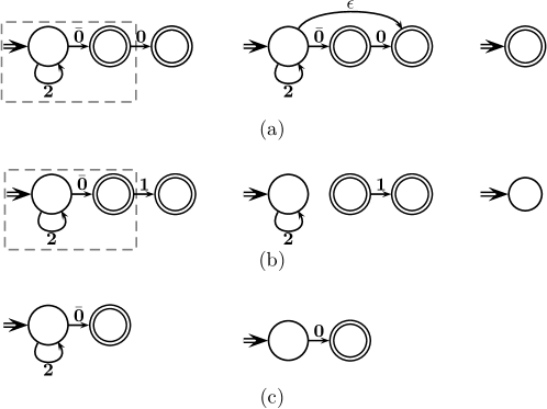
Figure 5. (a) & (b) show the simplification of the automaton $M_{\pi_{1}}^{\sigma}$ for the slicing criteria $\sigma=\{\epsilon,\mathbf{0}\}$ and $\sigma=\{\epsilon,\mathbf{1}\}$ respectively. (c) shows the canonical automaton ${A}_{\pi_{1}}$ and the corresponding completing automaton $\overline{A}_{\pi_{1}}$

We get around the problem of undecidability, we use the technique of Mohri-Nederhoff (Mohri and Nederhof, 2000) to over-approximate ${P}_{\pi}^{\sigma}$ by a strongly regular grammar. The NFA corresponding to this automaton is denoted as $M_{\pi}^{\sigma}$. The simplification rules can be applied on $M_{\pi}^{\sigma}$ without any loss of precision. The details of the simplification process are in (Karkare et al., 2007).

For our running example, the grammar after demand analysis is already regular, and thus remains unchanged by Mohri-Nederhoff transformation. The automata in Figures 5(a) and 5(b) correspond to the two slicing criteria $\sigma_{\mathbf{lcc}}=\{\epsilon,\mathbf{0}\}$ and $\sigma_{\mathbf{lcc}}=\{\epsilon,\mathbf{1}\}$ and illustrate the simplification of corresponding Mohri-Nederhoff automata $M_{\pi_{1}}^{\sigma_{\mathbf{lcc}}}$. It can be seen that, when the slicing criterion is $\{\epsilon,\mathbf{1}\}$, the language of $\mathsf{D}_{\pi_{1}}$ is empty and hence $e$ can be sliced away. A drawback of the method outlined above is that with a change in the slicing criterion, the entire process of grammar generation, Mohri-Nederhoff approximation and simplification has to be repeated. This is likely to be inefficient for large programs.

5. Incremental Slicing

We now present an incremental algorithm which avoids the repetition of computation when the same program is sliced with different criteria. This can be done by pre-computing the part of the slice computation that is independent of the slicing criterion. The pre-computed part can then be used efficiently to slice the program for a given slicing criterion.

In general, the pre-computation consists of three steps: (i) computing the demand at each expression $\pi\!:e$ for the fixed slicing criterion $\{\epsilon\}$ and applying the Mohri-Nederhoff procedure to yield the automaton ${M}_{\pi}^{\{\epsilon\}}$, (ii) a step called canonicalization which applies the simplification rules on ${M}_{\pi}^{\{\epsilon\}}$ until the $\bar{}\mathbf{0}$  and $\bar{}\mathbf{1}$ symbols in the strings accepted by the resulting automaton are only at the end, and, from this (iii) constructing an automaton called the completing automaton. For the running example, the canonicalized and the completing automata are shown Figures 5(c). We explain these steps now.

As stated earlier, the automaton ${M}_{\pi_{1}}^{\{\epsilon\}}$, after some simplifications, gives the first automaton (the canonicalized automaton) shown in Figure 5(c), which we shall denote ${A}_{\pi_{1}}$. It is clear that if ${A}_{\pi_{1}}$ is concatenated with a slicing criterion that starts with the symbol $\mathbf{0}$, the result, after simplification, will be non-empty. We call a string that starts with $\mathbf{0}$ as a completing string for ${A}_{\pi_{1}}$. In this case, detecting a completing string was easy because all strings accepted by ${A}_{\pi_{1}}$ end with $\bar{}\mathbf{0}$. Now consider the second automaton in Figure 5(c), called the completing automaton, that recognizes the language $\mathbf{0}(\mathbf{0}+\mathbf{1})^{\ast}$. This automaton recognizes all completing strings for ${A}_{\pi_{1}}$ and nothing else. Thus for an arbitrary slicing criterion $\sigma$, it suffices to intersect $\sigma$ with the completing automaton to decide whether the expression at $\pi_{1}$ will be in the slice. In fact, it is enough for the completing automaton to recognize just the language $\{\mathbf{0}\}$ instead of $\mathbf{0}(\mathbf{0}+\mathbf{1})^{\ast}$. The reason is that any slicing criterion, say $\sigma$, is prefix closed, and therefore $\sigma\cap\{\mathbf{0}\}$ is empty if and only if $\sigma\cap\mathbf{0}(\mathbf{0}+\mathbf{1})^{\ast}$ is empty. Our incremental algorithm generalizes this reasoning.

5.1. Completing Automaton and Slicing

For constructing the completing automaton for an expression $e$, we saw that it would be convenient to simplify the automaton ${M}_{e}^{\{\epsilon\}}$ to an extent that all accepted strings, after simplification, have $\bar{}\mathbf{0}$ and $\bar{}\mathbf{1}$ symbols only at the end. We now give a set of rules, denoted by $\mathcal{C}$, that captures this simplification.

$$\mathcal{C}(\{\epsilon\}) =\{\epsilon\}$$

$$\mathcal{C}(\mathbf{0}\sigma) =\mathbf{0}\mathcal{C}(\sigma)$$

$$\mathcal{C}(\mathbf{1}\sigma) =\mathbf{1}\mathcal{C}(\sigma)$$

$$\mathcal{C}(\bar{}\mathbf{0}\sigma) =\{\bar{}\mathbf{0}\mid\{\epsilon\}=\mathcal{C}(\sigma)\}\cup\{\alpha\mid\mathbf{0}\alpha\in\mathcal{C}(\sigma)\}$$

$$\cup\{\bar{}\mathbf{0}\bar{}\mathbf{1}\alpha\mid\bar{}\mathbf{1}\alpha\in\mathcal{C}(\sigma)\}\cup\{\bar{}\mathbf{0}\bar{}\mathbf{0}\alpha\mid\bar{}\mathbf{0}\alpha\in\mathcal{C}(\sigma)\}$$

$$\mathcal{C}(\bar{}\mathbf{1}\sigma) =\{\bar{}\mathbf{1}\mid\{\epsilon\}=\mathcal{C}(\sigma)\}\cup\{\alpha\mid\mathbf{1}\alpha\in\mathcal{C}(\sigma)\}$$

$$\cup\{\bar{}\mathbf{1}\bar{}\mathbf{1}\alpha\mid\bar{}\mathbf{1}\alpha\in\mathcal{C}(\sigma)\}\cup\{\bar{}\mathbf{1}\bar{}\mathbf{0}\alpha\mid\bar{}\mathbf{0}\alpha\in\mathcal{C}(\sigma)\}$$

$$\mathcal{C}({\mathbf{2}}\sigma) ={\mathbf{2}}\mathcal{C}(\sigma)$$

$$\mathcal{C}(\sigma_{1}\cup\sigma_{2}) =\mathcal{C}(\sigma_{1})\cup\mathcal{C}(\sigma_{2})$$

$\mathcal{C}$ differs from $\mathcal{S}$ in that it accumulates continuous run of $\bar{}\mathbf{0}$ and $\bar{}\mathbf{1}$  at the end of a string. Notice that $\mathcal{C}$, like $\mathcal{S}$, simplifies its input string from the right. Here is an example of $\mathcal{C}$ simplification:

$$\mathbf{1}{\mathbf{2}}\bar{}\mathbf{0}\mathbf{0}\mathbf{0}{\mathbf{2}}\mathbf{0}\bar{}\mathbf{1}\bar{}\mathbf{1}\mathbf{1}\bar{}\mathbf{0}\stackrel{{\scriptstyle\mathcal{C}}}{{\rightarrow}}\mathbf{1}{\mathbf{2}}\bar{}\mathbf{0}\mathbf{0}\mathbf{0}{\mathbf{2}}\mathbf{0}\bar{}\mathbf{1}\bar{}\mathbf{0}\stackrel{{\scriptstyle\mathcal{C}}}{{\rightarrow}}\mathbf{1}{\mathbf{2}}\mathbf{0}{\mathbf{2}}\mathbf{0}\bar{}\mathbf{1}\bar{}\mathbf{0}$$

In contrast the simplification of the same string using $\mathcal{S}$ gives:

$$\mathbf{1}{\mathbf{2}}\bar{}\mathbf{0}\mathbf{0}\mathbf{0}{\mathbf{2}}\mathbf{0}\bar{}\mathbf{1}\bar{}\mathbf{1}\mathbf{1}\bar{}\mathbf{0}\stackrel{{\scriptstyle\mathcal{S}}}{{\rightarrow}}\mathbf{1}{\mathbf{2}}\bar{}\mathbf{0}\mathbf{0}\mathbf{0}{\mathbf{2}}\mathbf{0}\bar{}\mathbf{1}\bar{}\mathbf{1}\mathbf{1}\emptyset\stackrel{{\scriptstyle\mathcal{S}}}{{\rightarrow}}\mathbf{1}{\mathbf{2}}\bar{}\mathbf{0}\mathbf{0}\mathbf{0}{\mathbf{2}}\mathbf{0}\bar{}\mathbf{1}\bar{}\mathbf{0}\emptyset\stackrel{{\scriptstyle\mathcal{S}}}{{\rightarrow}}\ldots\stackrel{{\scriptstyle\mathcal{S}}}{{\rightarrow}}\emptyset$$

$\mathcal{C}$ satisfies two important properties:

Property 1.

The result of $\mathcal{C}$ always has the form $(\mathbf{0}+\mathbf{1}+{\mathbf{2}})^{\ast}(\bar{}\mathbf{0}+\bar{}\mathbf{1})^{\ast}$. Further, if $\sigma\subseteq(\mathbf{0}+\mathbf{1}+{\mathbf{2}})^{\ast}$, then $\mathcal{C}(\sigma)=\sigma$.

Property 2.

$\mathcal{S}$ subsumes $\mathcal{C}$, i.e., $\mathcal{S}(\mathcal{C}(\sigma_{1})\mathcal{C}(\sigma_{2}))=\mathcal{S}(\sigma_{1}\sigma_{2})$.

Note that while we have defined canonicalization over a language, the actual canonicalization takes place over an automaton—specifically the automaton ${M}_{\pi}$ obtained after the Mohri-Nederhoff transformation. The function createCompletingAutomaton in Algorithm 1 takes ${A}_{\pi}$, the canonicalized Mohri-Nederhoff automaton for the slicing criterion $\{\epsilon\}$, as input, and constructs the completing automaton, denoted as $\overline{A}_{\pi}$.

Function createCompletingAutomaton($A$)

      Data: The Canonicalized Automaton $A=\left\langle Q,\{\mathbf{0},\mathbf{1},\bar{}\mathbf{0},\bar{}\mathbf{1},{\mathbf{2}}\},\delta,q_{0},F\right\rangle$

      Result: $\overline{A}$, the completing automaton for $A$

     

     $F^{\prime}\leftarrow\{q_{\rm fr}\mid q_{\rm fr}\in Q,\,\textnormal{{hasBarFreeTransition}}(q_{0},q_{\rm fr},\delta)\}$

     

     /* Reverse the ‘‘bar’’ transitions: directions as well as labels */

      foreach (transition $\delta(q,\bar{}\mathbf{0})\rightarrow q^{\prime}$) do

           add transition $\delta^{\prime}(q^{\prime},\mathbf{0})\rightarrow q$

           foreach (transition $\delta(q,\bar{}\mathbf{1})\rightarrow q^{\prime}$) do

                add transition $\delta^{\prime}(q^{\prime},\mathbf{1})\rightarrow q$

                $q^{\prime}_{0}\leftarrow$ new state /* start state of $\overline{A}$ */

                foreach (state $q\in F$)  do

                     add transition $\delta^{\prime}(q^{\prime}_{0},\epsilon)\rightarrow q$

                    

                    return $\left\langle Q\cup\{q^{\prime}_{0}\},\{\mathbf{0},\mathbf{1}\},\delta^{\prime},q^{\prime}_{0},F^{\prime}\right\rangle$

                     Function inSlice(e, $\sigma$)

                          Data: expression e, slicing criteria $\sigma$

                          Result: Decides whether e should be retained in slice

                          return $(\mathsf{L}({\overline{A}_{\textnormal{{e}}}})\cap\ \textnormal{{$\sigma$}}\neq\emptyset)$

Algorithm 1 Functions to create the completing automaton and the slicing function.

Recollect that the strings recognized by ${A}_{\pi}$ are of the form $(\mathbf{0}+\mathbf{1}+{\mathbf{2}})^{\ast}(\bar{}\mathbf{0}+\bar{}\mathbf{1})^{\ast}$. The algorithm first computes the set of states reachable from the start state using only edges with labels $\{\mathbf{0},\mathbf{1},{\mathbf{2}}\}$. This set is called the frontier set. It then complements the automaton and drops all edges with $\{\mathbf{0},\mathbf{1},{\mathbf{2}}\}$ labels. Finally, all states in the frontier set are marked as final states. Since $A_{\pi}$ is independent of the slicing criteria, the completing automaton is also independent of the slicing criteria and needs to be computed only once. It can be stored and re-used whenever the program needs to be sliced. To decide whether $\pi\!\!:e$ can be sliced out, the function inSlice described in Algorithm 1 just checks if the intersection of the slicing criteria with $\mathsf{L}({\overline{A}_{\pi}})$ is null.

5.2. Correctness of Incremental Slicing

We now show that the incremental algorithm to compute incremental slices is correct. Recall that we use the following notations: (i) ${G}_{\pi}^{\sigma}$ is the grammar generated by demand analysis (Figure 4) for an expression $\pi\!\!:e$ in the program of interest, when the slicing criteria is $\sigma$, (ii) $A_{\pi}$ is the automaton corresponding to ${G}_{\pi}^{\{\epsilon\}}$ after Mohri-Nederhoff transformation and canonicalization, and (iii) $\overline{A}_{\pi}$ is the completing automaton for $e$. We first show that the result of the demand analysis for an arbitrary slicing criterion $\sigma$ can be decomposed as the concatenation of the demand analysis obtained for the fixed slicing criterion $\{\epsilon\}$ and $\sigma$ itself.

Lemma 5.1.

For all expressions $e$ and slicing criteria $\sigma$, $\mathsf{L}({{G}_{\pi}^{\sigma}})$ = $\mathsf{L}({{G}_{\pi}^{\{\epsilon\}}})\sigma$.

Proof.

The proof is by induction on the structure of $e$. Observe that all the rules of the demand analysis (Figure 4) add symbols only as prefixes to the incoming demand. Hence, the slicing criteria will always appear as a suffix of any string that is produced by the grammar. Thus, any grammar $\mathsf{L}({{G}_{\pi}^{\sigma}})$ can be decomposed as $\sigma^{\prime}\sigma$ for some language $\sigma^{\prime}$. Substituting $\{\epsilon\}$ for $\sigma$, we get ${G}_{\pi}^{\{\epsilon\}}=\sigma^{\prime}$. Thus $\mathsf{L}({{G}_{\pi}^{\sigma}})$ = $\mathsf{L}({{G}_{\pi}^{\{\epsilon\}}})\sigma$. ∎

Given a string $s$ over $(\bar{}\mathbf{0}+\bar{}\mathbf{1})^{\ast}$, we use the notation $\overline{s}$ to stand for the reverse of $s$ in which all occurrences of $\bar{}\mathbf{0}$ are replaced by $\mathbf{0}$ and $\bar{}\mathbf{1}$ replaced by $\mathbf{1}$. Clearly, $\mathcal{S}(\{s\overline{s}\})=\{\epsilon\}$.

We next prove the completeness and minimality of $\overline{A}_{\pi}$.

Lemma 5.2.

$\{s\mid\mathcal{S}(\mathsf{L}({M_{\pi}^{\{s\}}}))\neq\ \emptyset\}=\mbox{$\mathsf{L}({\overline{A}_{\pi}})(\mathbf{0}+\mathbf{1})^{\ast}$}$

Proof.

We first prove $LHS\ \subseteq\ RHS$. Let the string $s\in\mathcal{S}(\mathsf{L}({M_{\pi}^{\{s\}}}))$. Then by Lemma 5.1, $s\in\mathcal{S}(\mbox{$\mathsf{L}({M_{\pi}^{\{\epsilon\}}})\{s\}$})$. By Property 2, this also means that $s\in\mathcal{S}(\mbox{$\mathcal{C}(\mathsf{L}({M_{\pi}^{\{\epsilon\}}}))\{s\}$})$. Since strings in $\mathcal{C}(\mathsf{L}({M_{\pi}^{\{\epsilon\}}}))$ are of the form $(\mathbf{0}+\mathbf{1}+{\mathbf{2}})^{\ast}(\bar{}\mathbf{0}+\bar{}\mathbf{1}))^{\ast}$ (Property 1), this means that there is a string $p_{1}p_{2}$ such that $p_{1}\in(\mathbf{0}+\mathbf{1}+{\mathbf{2}})^{\ast}$ and $p_{2}\in(\bar{}\mathbf{0}+\bar{}\mathbf{1})^{\ast}$, and $\mathcal{S}(\{p_{2}\}\{s\})\ \subseteq(\mathbf{0}+\mathbf{1})^{\ast}$. Thus $s$ can be split into two strings $s_{1}$ and $s_{2}$, such that $\mathcal{S}(\mbox{$\{p_{2}\}\{s_{1}\}$})=\{\epsilon\}$. Therefore $s_{1}=\overline{p_{2}}$. From the construction of $\overline{A}_{\pi}$ we have $\overline{p_{2}}\in\mathsf{L}({\overline{A}_{\pi}})$ and $s_{2}\ \in\ (\mathbf{0}+\mathbf{1})^{\ast}$. Thus, $s\ \in\mbox{$\mathsf{L}({\overline{A}_{\pi}})(\mathbf{0}+\mathbf{1})^{\ast}$}$.

Conversely, for the proof of $RHS\ \subseteq\ LHS$, we assume that a string $s\in\mbox{$\mathsf{L}({\overline{A}_{\pi}})(\mathbf{0}+\mathbf{1})^{\ast}$}$. From the construction of $\overline{A}_{\pi}$ we have strings $p_{1},p_{2},s^{\prime}$ such that $p_{1}p_{2}\in\mathcal{C}(\mathsf{L}({M_{\pi}^{\epsilon}}))$, $p_{1}\in(\mathbf{0}+\mathbf{1}+{\mathbf{2}})^{\ast}$, $p_{2}\in(\bar{}\mathbf{0}+\bar{}\mathbf{1})^{\ast}$, $s$ is $\overline{p_{2}}s^{\prime}$ and $s^{\prime}\in(\mathbf{0}+\mathbf{1})^{\ast}$. Thus, $\mathcal{S}(\mathsf{L}({M_{\pi}^{\{s\}}}))=\mathcal{S}(\mathsf{L}({\mbox{$M_{\pi}^{\{\epsilon\}}\{s\}$}}))=\mathcal{S}(\mbox{$\mathcal{C}(\mathsf{L}({M_{\pi}^{\{\epsilon\}}})){\{s\}})$}=\mathcal{S}(\{\mbox{$p_{1}\mbox{$p_{2}\mbox{$\overline{p_{2}}s^{\prime}$}$}$}\})=\{p_{1}s^{\prime}\}$. Thus, $\mathcal{S}(\mathsf{L}({M_{\pi}^{\{s\}}}))$ is non-empty and $s\in LHS$. ∎

We now prove our main result: Our slicing algorithm represented by inSlice (Algorithm 1) returns true if and only if $\mathcal{S}$($\mathsf{L}({A_{\pi}^{\epsilon}})\sigma$) is non-empty.

Theorem 5.3.

$\mathcal{S}(\mathsf{L}({M_{\pi}^{\sigma}}))\neq\emptyset\leftrightarrow\ \mbox{\bf inSlice}(e,\sigma)$

Proof.

We first prove the forward implication. Let $s\in\mathcal{S}(\mathsf{L}({M_{\pi}^{\sigma}}))$. From Lemma 5.1, $s\in\mathcal{S}(\mbox{$\mathsf{L}({M_{\pi}^{\epsilon}})\sigma$})$. From Property 2, $s\in\mathcal{S}(\mbox{$\mathcal{C}(\mathsf{L}({M_{\pi}^{\epsilon}}))\sigma$})$. Thus, there are strings $p_{1},p_{2}$ such that $p_{1}\in\mathcal{C}(\mathsf{L}({M_{\pi}^{\epsilon}})),\ p_{2}\in\sigma,s=\mathcal{S}(\{p_{1}p_{2}\})$. Further $p_{1}$ in turn can be decomposed as $p_{3}p_{4}$ such that $p_{3}\in(\mathbf{0}+\mathbf{1}+{\mathbf{2}})^{\ast}$ and $p_{4}\in(\bar{}\mathbf{0}+\bar{}\mathbf{1})^{\ast}$. We also have $\mathcal{S}(\{p_{4}p_{2}\})\subseteq(\mathbf{0}+\mathbf{1})^{\ast}$. Thus $\overline{p_{4}}$ is a prefix of $p_{2}$.

From the construction of $\overline{A}_{\pi}$, we know $\overline{p_{4}}\in\mathsf{L}({\overline{A}_{\pi}})$. Further, $\overline{p_{4}}$ is a prefix of $p_{2}$ and $p_{2}\in\sigma$, from the prefix closed property of $\sigma$ we have $\overline{p_{4}}\in\sigma$. This implies $\overline{A}_{\pi}\cap\sigma\neq\emptyset$ and thus $\mbox{\bf inSlice}(e,\sigma)$ returns true.

Conversely, if $\mbox{\bf inSlice}(e,\sigma)$ is true, then $\exists s:s\in\mathsf{L}({\overline{A}_{\pi}})\cap\sigma$. In particular, $s\in\mathsf{L}({\overline{A}_{\pi}})$. Thus, from Lemma 5.2 we have $\mathcal{S}(\mathsf{L}({M_{\pi}^{\{s\}}}))\neq\emptyset$. Further, since $s\in\sigma$ we have $\mathcal{S}(\mathsf{L}({M_{\pi}^{\sigma}}))\neq\emptyset$.∎

6. Extension to higher order functions

($\mathbf{define}$ ($\mathbf{hof}$ f l)       ($\mathbf{return}$ $\pi$:(f l)))

($\mathbf{define}$ ($\mathbf{foldr}$ $\mathbf{f}$ id l)       ($\mathbf{if}$($\mathbf{null?}$ l)) ($\mathbf{return}$ id)         ($\mathbf{return}$ ($\mathbf{f}$ ($\mathbf{car}$ l)                     ($\mathbf{foldr}$ $\mathbf{f}$ id ($\mathbf{cdr}$ l)))))

($\mathbf{define}$ ($\mathbf{fun}$ x y)       ($\mathbf{return}$ (+ y 1)))

($\mathbf{define}$ ($\mathbf{main}$)       $(\mbox{$\mathbf{let}$}\ \mbox{\tt lst1}\ \leftarrow$ ($\mathbf{cons}$ a ($\mathbf{cons}$ b $\mathbf{nil}$)) $\mathbf{in}$         $(\mbox{$\mathbf{let}$}\ \mathbf{g}\ \leftarrow$ ($\mathbf{foldr}$ $\mathbf{fun}$ 0) $\mathbf{in}$           $(\mbox{$\mathbf{return}$}\ (\mbox{$\mathbf{cons}$}\ (\mathbf{hof}~{}\mbox{$\mathbf{car}$}~{}\mbox{\tt lst1})$           $\phantom{(\mbox{$\mathbf{return}$}\ (\mbox{$\mathbf{cons}$}\ }(\mathbf{hof}~{}\mathbf{g}~{}\mbox{\tt lst1})))))$

(a) A program with higher order functions

($\mathbf{define}$ ($\mathbf{hof\_g}$ l)       ($\mathbf{return}$ $\pi_{f}$:($\mathbf{foldr\_fun}$ 0 l)))

($\mathbf{define}$ ($\mathbf{hof\_car}$ l)       ($\mathbf{return}$ $\pi_{c}$:($\mathbf{car}$ l)))

($\mathbf{define}$ ($\mathbf{foldr\_fun}$ id l)       ($\mathbf{if}$($\mathbf{null?}$ l)) ($\mathbf{return}$ id)         ($\mathbf{return}$ ($\mathbf{fun}$ ($\mathbf{car}$ l)                     ($\mathbf{foldr\_fun}$ id ($\mathbf{cdr}$ l)))))

($\mathbf{define}$ ($\mathbf{fun}$ x y)       ($\mathbf{return}$ (+ y 1)))

($\mathbf{define}$ ($\mathbf{main}$)       $(\mbox{$\mathbf{let}$}\ \mbox{\tt lst1}\ \leftarrow$ ($\mathbf{cons}$ a ($\mathbf{cons}$ b $\mathbf{nil}$)) $\mathbf{in}$         $(\mbox{$\mathbf{let}$}\ \mathbf{g}\ \leftarrow$ ($\mathbf{foldr\_fun}$ 0) $\mathbf{in}$           $(\mbox{$\mathbf{return}$}\ (\mbox{$\mathbf{cons}$}\ (\mathbf{hof\_car}~{}\mbox{\tt lst1})$           $\phantom{(\mbox{$\mathbf{return}$}\ (\mbox{$\mathbf{cons}$}\ }(\mathbf{hof\_g}~{}\mbox{\tt lst1}))))))$

(b) Program in (a) after specialization.

($\mathbf{define}$ ($\mathbf{hof}$ f l)       ($\mathbf{return}$ $\pi$:(f l))) $(\mbox{$\mathbf{define}$}\ (\mathbf{main})$       $(\mbox{$\mathbf{let}$}\ \mbox{\tt lst1}\ \leftarrow$ ($\mathbf{cons}$ a $\square$) $\mathbf{in}$         $(\mbox{$\mathbf{let}$}\ \mathbf{g}\ \leftarrow$ $\square$) $\mathbf{in}$           $(\mbox{$\mathbf{return}$}\ (\mbox{$\mathbf{cons}$}\ (\mathbf{hof}~{}\mbox{$\mathbf{car}$}~{}\mbox{\tt lst1})$           $\phantom{(\mbox{$\mathbf{return}$}\ (\mbox{$\mathbf{cons}$}\ }\square))))$

(c) Slice of the program in (a) with   slicing criterion $\{\epsilon,\mathbf{0}\}$.

Figure 6. An example higher order program

We now describe how our method can also be used to slice higher order programs. This section has been included mainly for completeness, and we do not make claims of novelty. We handle all forms of higher-order functions except the cases of functions being returned as a result, and functions being stored in data structures—in our case lists. Even with these limitations, one can write a number of useful and interesting higher-order programs in our language.

Consider the program in Figure 6(a). It contains a higher order function $\mathbf{hof}$ which applies its first argument f on its second argument l. The function $\mathbf{main}$ creates a list lst1 and a function value g (through partial application) and uses these in the two calls to $\mathbf{hof}$. Finally, $\mathbf{main}$  returns the result of these calls in a pair. The program exhibits higher order functions that take as actual arguments both manifest functions and partial applications.

For our first-order method to work on higher order functions, we borrow from a technique called firstification (Mitchell and Runciman, 2009; Reynolds, 1998). Firstification transforms a higher-order program to a first-order program without altering its semantics. Our version of firstification repeatedly (i) finds for each higher-order function the bindings of each of its functional parameters, (ii) replaces the function by a specialized version for each of the bindings, and (iii) replaces each application of f by its specialized version. These steps are repeated till we we are left with a program containing first order functions only. In the example being considered, we first discover that f in foldr has a single binding to fun and the f of hof has a binding to car. Specialization gives the functions foldr_fun and hof_car. We now see that f of hof has a second binding to the partial application (foldr fun), This gives rise to a second specialization of hof called hof_g.

The program after firstification is shown in Figure 6(b). This program is subjected to demand analysis and the results are reflected back into the higher-order program. Inside a higher order function that has been specialized, the demand on an expression is an union of the demands on the specialized versions of the expression. Thus, the demand on $\pi$ is given by the union of the demands on $\pi_{c}$ and $\pi_{f}$. Where the higher order function is applied, the demand on its arguments is derived from the demand transformer of its specialized version. As an example, the demand on lst1 in (hof car lst1) is obtained from the demand transformers of hof_car. For the slicing criterion $\{\epsilon,\mathbf{0}\}$, the the demand on the second argument of (cons (hof car lst1) (hof g lst1)) is null and thus this argument and the binding of g can both be sliced away. The slice for $\{\epsilon,\mathbf{0}\}$ is shown in Figure 6(c).

Note that our simple firstifier requires us to statically find all bindings of a functional parameter. This is not possible if we allow functions to be returned as results or store functions in data-structures. As an example we can consider a function $f$, that, depending on a calculated value $n$, returns a function $g$ iterated $n$ times (i.e. $g\circ g\;\circ\stackrel{{\scriptstyle n~{}\mathit{times}}}{{\ldots}}\circ\;g$). A higher-order function receiving this value as a parameter would be cannot be specialized using the techniques described, for example, in (Mitchell and Runciman, 2009). A similar thing can happen if we allow functions in lists.

Table 1. Statistics for incremental and non-incremental slicing

Program	Pre-	#exprs	Slicing with $\{\epsilon\}$			Slicing with $\{\epsilon,0\}$			Slicing with $\{\epsilon,1\}$
	comput ation	in program	Non-inc time (ms)	Inc time (ms)	#expr in slice	Non-inc time (ms)	Inc time (ms)	#expr in slice	Non-inc time (ms)	Inc time (ms)	#expr in slice
First-order Programs
treejoin	6900.0	581	6163.2	2.4	536	5577.2	2.8	538	5861.4	4.6	538
deriv	399.6	389	268.0	1.6	241	311.2	1.6	249	333.2	2.3	266
paraffins	3252.8	1152	2287.3	5.2	1067	2529.2	5.1	1067	2658.7	5.1	1067
nqueens	395.4	350	309.9	1.5	350	324.6	1.5	350	328.1	1.6	350
minmaxpos	27.9	182	18.1	0.9	147	19.5	0.8	149	20.5	0.9	149
nperm	943.1	590	627.4	2.1	206	698.4	11.2	381	664.0	11.8	242
linecharcount​​	11.7	91	7.0	0.5	69	7.5	0.5	78	7.4	0.5	82
studentinfo	1120.6	305	858.2	1.2	96	854.6	1.3	101	1043.3	7.5	98
knightstour	2926.5	630	2188.1	2.8	436	2580.6	12.2	436	2492.8	7.4	436
takl	71.6	151	46.1	0.7	99	49.5	0.8	105	48.5	0.7	99
lambda	4012.9	721	3089.0	2.7	26	3377.4	13.2	705	2719.8	5.3	33
Higher-order Programs
parser	60088.2	820	46066.8	2.3	203	45599.0	2.3	209	61929.2	4.1	209
maptail	22.1	96	5.5	0.5	51	15.4	0.6	67	17.4	0.6	56
fold	21.4	114	13.3	0.4	17	14.4	0.5	76	16.9	0.6	33

7. Experiments and results

In this section, we present the results from our experiments on the implementations of both versions of slicing. In the absence of the details of implementations of other slicing methods, we have compared the incremental step of our method with the non-incremental version. Our experiments show that the incremental slicing algorithm gives benefits even when the overhead of creating the completing automata is amortized over even a few slicing criteria.

Our benchmarks consists of first order programs derived from the nofib suite (NoFib, 2017). The higher order programs have been handcrafted to bring out the issues related to higher order slicing. The program named parser includes most of the higher order parser combinators required for parsing. fold corresponds to the example in Figure 6. Table 1 shows the time required for slicing with different slicing criteria. For each benchmark, we first show, the pre-computation time, i.e. the time required to construct the completing automata. We then consider three different slicing criteria, and for each slicing criterion, present the times for non-incremental slicing and the incremental step. The results in Table 1 show that for all benchmarks, the time required to compute the completing automata is comparable to the time taken for computing the slice non-incrementally. Since computing completing automata is a one time activity, incremental slicing is very efficient even when a program is sliced only twice. As seen in Table 1, the time taken for the incremental step is orders of magnitude faster than non-incremental slicing, thus confirming the benefits of reusing the completing automata.

We also show the number of expressions in the original program and in the slice produced to demonstrate the effectiveness of the slicing process itself. Here are some of the interesting cases. It can be seen that the slice for nqueens for any slicing criterion includes the entire program. This is because finding out whether a solution exists for nqueens requires the entire program to be executed. On the other hand, the program lambda is a $\lambda$-expression evaluator that returns a tuple consisting of an atomic value and a list. The criterion $\{\epsilon,0\}$ requires majority of the expressions in the program to be present in the slice to compute the atomic value. On the other hand, the criterion $\{\epsilon\}$ or $\{\epsilon,1\}$ do not require any value to be computed and expressions which compute the constructor only are kept in the slice, hence our algorithm is able to discard most of the expressions. This behavior can be clearly seen in the higher-order example fold where a slicing criterion $\{\epsilon,\mathbf{0}\}$ selects an expression which only uses the first element of lst1, thus allowing our slicing algorithm to discard most of the expressions that construct lst1. After examining the nature of the benchmark programs, the slicing criteria and the slices, we conclude that slicing is most effective when the slicing criterion selects parts of a bounded structure, such as a tuple, and the components of the tuple are produced by parts of the program that are largely disjoint.

8. Related work

Program slicing has been an active area of research. However, most of the efforts in slicing have been for imperative programs. The surveys (Tip, 1995; Binkley and Harman, 2004; Silva, 2012) give good overviews of the variants of the slicing problem and their solution techniques. The discussion in this section will be centered mainly around static and backward slicing of functional programs.

In the context of imperative programs, a slicing criterion is a pair consisting of a program point, and a set of variables. The slicing problem is to determine those parts of the program that decide the values of the variables at the program point (Weiser, 1984). A natural solution to the slicing problem is through the use of data and control dependences between statements. Thus the program to be sliced is transformed into a graph called the program dependence graph (PDG) (Ottenstein and Ottenstein, 1984; Horwitz et al., ), in which nodes represent individual statements and edges represent dependences between them. The slice consists of the nodes in the PDG that are reachable through a backward traversal starting from the node representing the slicing criterion. Horwitz, Reps and Binkley (Horwitz et al., ) extend PDGs to handle interprocedural slicing. They show that a naive extension could lead to imprecision in the computed slice due to the incorrect tracking of the calling context. Their solution is to construct a context-independent summary of each function through a linkage grammar, and then use this summary to step across function calls. The resulting graph is called a system dependence graph (SDG). Our method generalizes SDGs to additionally keep track of the construction of algebraic data types ($\mathbf{cons}$), selection of components of data types ($\mathbf{car}$ and $\mathbf{cdr}$) and their interaction, which may span across functions.

Silva, Tamarit and Tomás  (Silva et al., 2012) adapt SDGs for functional languages, in particular Erlang. The adaptation is straightforward except that they handle dependences that arise out of pattern matching. Because of the use of SDGs, they can manage calling contexts precisely. However, as pointed out by the authors themselves, when given the Erlang program: {$\mathbf{main}$() -> x = {1,2}, {y,z} = x, y}, their method produces the imprecise slice {$\mathbf{main}$()  ->  x = {1,2}, {y,$\square$} = x, y} when sliced on the variable y. Notice that the slice retains the constant 2, and this is because of inadequate handling of the interaction between $\mathbf{cons}$ and $\mathbf{cdr}$. For the equivalent program ($\mathbf{let}$  x$\leftarrow$   ($\mathbf{cons}$ 1 2)  $\mathbf{in}$  ($\mathbf{let}$  y  $\leftarrow$  ($\mathbf{car}$  x)  $\mathbf{in}$  y)) with the slicing criterion $\epsilon$, our method would correctly compute the demand on the constant 2 as $\bar{}\mathbf{1}(\epsilon\cup\mathbf{0})$. This simplifies to the demand $\emptyset$, and 2 would thus not be in the slice. Another issue is that while the paper mentions the need to handle higher order functions, it does not provide details regarding how this is actually done. This would have been interesting considering that the language considered allows lambda expressions.

The slicing technique that is closest to ours is due to Reps and Turnidge (Reps and Turnidge, 1996). They use projection functions, represented as certain kinds of tree grammars, as slicing criteria. This is the same as our use of prefix-closed regular expressions. Given a program P and a projection function $\psi$, their goal is to produce a program which behaves like $\psi\circ\emph{P}$. The analysis consists of propagating the projection function backwards to all subexpressions of the program. After propagation, any expression with the projection function $\bot$ (corresponding to our $\emptyset$ demand), are sliced out of the program. Liu and Stoller (Liu and Stoller, 2003) also use a method that is very similar to (Reps and Turnidge, 1996), but more extensive in scope.

These techniques differ from ours in two respects. These methods, unlike ours, do not derive context-independent summaries of functions. This results in a loss of information due to merging of contexts and affects the precision of the slice. Moreover, the computation of function summaries using symbolic demands enables the incremental version of our slicing method. Consider, as an example, the program fragment $\pi\!\!:\!(\mbox{$\mathbf{cons}$}~{}\pi_{1}\!\!:\!x~{}\pi_{2}\!\!:\!y)$ representing the body of a function. Demand analysis with the symbolic demand $\sigma$ gives the demand environment $\left\{\pi\mapsto\sigma,\pi_{1}\mapsto\bar{}\mathbf{0}\sigma,\pi_{2}\mapsto\bar{}\mathbf{1}\sigma\right\}$. Notice that the demands $\pi_{1}$ and $\pi_{2}$ are in terms of the symbols $\bar{}\mathbf{0}$ and $\bar{}\mathbf{1}$. This is a result of our decision to work with symbolic demands, and, as a consequence, also handle the constructor-selector interaction symbolically. If we now slice with the default criterion $\epsilon$ and then canonicalize (instead of simplify), we are left with the demand environment $\left\{\pi\mapsto\epsilon,\pi_{1}\mapsto\bar{}\mathbf{0},\pi_{2}\mapsto\bar{}\mathbf{1}\right\}$. Notice that there is enough information in the demand environment to deduce, through the construction of the completing automaton, that $\pi_{1}$ ($\pi_{2}$) will be in the slice only if the slicing criterion includes $\mathbf{0}$($\mathbf{1}$). Since the methods in (Reps and Turnidge, 1996) and (Liu and Stoller, 2003) deal with demands in their concrete forms, it is difficult to see the incremental version being replayed with their methods.

There are other less related approaches to slicing. A graph based approach has also been used by Rodrigues and Barbosa (Rodrigues and Barbosa, 2006a) for component identification in Haskell programs. Given the intended use, the nodes of the graph represents coarser structures such as modules, functions and data type definitions, and the edges represents relations such as containment (e.g. a module containing a function definition). On a completely different note, Rodrigues and Barbosa (Rodrigues and Barbosa, 2006b) use program calculation in the Bird-Meerteens formalism for obtaining a slice. Given a program $P$ and a projection function $\psi$, they calculate a program which is equivalent to $\psi\circ\emph{P}$. However the method is not automated. Finally, dynamic slicing techniques have been explored for functional programs by Perera et al. (Perera et al., ), Ochoa et al. (Ochoa et al., 2008) and Biswas (Biswas, 1997).

9. Conclusions and Future Work

We have presented a demand-based algorithm for incremental slicing of functional programs. The slicing criterion is a prefix-closed regular language and represents parts of the output of the program that may be of interest to a user of our slicing method. We view the slicing criterion as a demand, and the non-incremental version of the slicer does a demand analysis to propagate this demand through the program. The slice consists of parts of the program with non-empty demands after the propagation. A key idea in this analysis is the use of symbolic demands in demand analysis. Apart form better handling of calling contexts that improves the precision of the analysis, this also helps in building the incremental version.

The incremental version builds on the non-incremental version. A per program pre-computation step slices the program with the default criterion $\epsilon$. This step factors out the computation that is common to slicing with any criterion. The result, reduced to a canonical form, can now be used to find the slice for a given criterion with minimal computation. We have proven the correctness of the incremental algorithm with respect to the non-incremental version. And finally, we have extended our approach to higher-order programs through firstification. Experiments with our implementation confirm the benefits of incremental slicing.

There are however two areas of concern, one related to efficiency and the other to precision. To be useful, the slicer should be able to slice large programs quickly. While our incremental slicer is fast enough, the pre-computation step is slow, primarily because of the canonicalization step. In addition, the firstification process may create a large number of specialized first-order programs. As an example, our experiments with functional parsers show that the higher-order parser combinators such as or-parser and the and-parser are called often, and the arguments to these calls are in turns calls to higher order functions, for instance the Kleene closure and the positive closure parsers.

($\mathbf{define}$ ($\mathbf{mapsq}$ l)

($\mathbf{if}$($\mathbf{null?}$ l) ($\mathbf{return}$ l)

($\mathbf{return}$ ($\mathbf{cons}$ ($\mathbf{sq}$ ($\mathbf{car}$ l))

($\mathbf{mapsq}$ ($\mathbf{cdr}$ l)))))

Figure 7. Example to illustrate the imprecision due to Mohri-Nederhoff approximation

The other concern is that while our polyvariant approach through computation of function summaries improves precision, the resulting analysis leads to an undecidable problem. The workaround involves an approximation that could lead to imprecision. As an example, consider the function $\mathbf{mapsq}$ shown in Figure 7. The reader can verify that the function summary for $\mathbf{mapsq}$ would be given as: $\mathds{DS}_{\mathit{\mathbf{mapsq}}}^{1}({\mathit{\sigma}})=\mbox{$\mathsf{DS}_{\mathit{\mathbf{mapsq}}}^{1}\sigma$}$, where $\mathsf{DS}_{\mathit{\mathbf{mapsq}}}^{1}$ is the language $\epsilon\mid\mathbf{1}^{n}\bar{}\mathbf{1}^{n}\mid\mathbf{1}^{n}\mathbf{0}{\mathbf{2}}\bar{}\mathbf{0}\bar{}\mathbf{1}^{n}$, for $n\geq 0$. Now, given a slicing criterion $\sigma=\{\epsilon,\mathbf{1},\mathbf{1}\mathbf{1},\mathbf{1}\mathbf{1}\mathbf{0}\}$ standing for the path to the third element of a list, it is easy to see that $\mathds{DS}_{\mathit{\mathbf{mapsq}}}^{1}({\mathit{\sigma}})$ after simplification would give back $\sigma$ itself, and this is the most precise slice. However, due to Mohri-Nederhoff approximation $\mathsf{DS}_{\mathit{\mathbf{mapsq}}}^{1}$ would be approximated by $\epsilon\mid\mathbf{1}^{n}\bar{}\mathbf{1}^{m}\mid\mathbf{1}^{k}\mathbf{0}{\mathbf{2}}\bar{}\mathbf{0}\bar{}\mathbf{1}^{l}$, $n$, $m$, $k$, $l$ $\geq 0$. In this case, $\mathsf{DS}_{\mathit{\mathbf{mapsq}}}^{1}$ would be $(\mathbf{0}+\mathbf{1})^{*}$, keeping all the elements of the input list l in the slice.

References

- (1)
- (2) Rahul Asati, Amitabha Sanyal, Amey Karkare, and Alan Mycroft. Liveness-Based Garbage Collection. In Compiler Construction - 23rd International Conference, CC 2014.
- Binkley and Harman (2004) David Binkley and Mark Harman. 2004. A survey of empirical results on program slicing. Advances in Computers 62 (2004).
- Biswas (1997) Sandip Kumar Biswas. 1997. Dynamic Slicing in Higher-order Programming Languages. Ph.D. Dissertation. University of Pennsylvania, Philadelphia, PA, USA.
- Chakravarty et al. (2003) Manuel M. T. Chakravarty, Gabriele Keller, and Patryk Zadarnowski. 2003. A Functional Perspective on SSA Optimisation Algorithms. In COCV, 2003.
- (6) Susan Horwitz, Thomas W. Reps, and David Binkley. Interprocedural Slicing Using Dependence Graphs. In Proceedings of the ACM SIGPLAN’88 Conference on Programming Language Design and Implementation (PLDI) 1988.
- Karkare et al. (2007) Amey Karkare, Uday Khedker, and Amitabha Sanyal. 2007. Liveness of Heap Data for Functional Programs. In Heap Analysis and Verification, HAV 2007.
- Kumar et al. (2016) Prasanna Kumar, Amitabha Sanyal, and Amey Karkare. 2016. Liveness-based Garbage Collection for Lazy Languages. In Inrenational Symposium on Memory Management (ISMM 2016).
- Liu and Stoller (2003) Yanhong A. Liu and Scott D. Stoller. 2003. Eliminating Dead Code on Recursive Data. Sci. Comput. Program. 47 (2003).
- Mitchell and Runciman (2009) Neil Mitchell and Colin Runciman. 2009. Losing Functions Without Gaining Data: Another Look at Defunctionalisation. In Proceedings of the 2nd ACM SIGPLAN Symposium on Haskell.
- Mohri and Nederhof (2000) Mehryar Mohri and Mark-Jan Nederhof. 2000. Regular Approximation of Context-Free Grammars through Transformation. In Robustness in Language and Speech Technology. Kluwer Academic Publishers.
- NoFib (2017) NoFib. 2017. Haskell Benchmark Suite. http://git.haskell.org/nofib.git. (Feb 2017). (Last accessed).
- Ochoa et al. (2008) Claudio Ochoa, Josep Silva, and Germán Vidal. 2008. Dynamic Slicing of Lazy Functional Programs Based on Redex Trails. Higher Order Symbol. Comput. 21 (2008).
- Ottenstein and Ottenstein (1984) Karl J. Ottenstein and Linda M. Ottenstein. 1984. The program dependence graph in a software development environment. ACM SIGPLAN Notices 19 (1984).
- (15) Roly Perera, Umut A. Acar, James Cheney, and Paul Blain Levy. Functional programs that explain their work. In ACM SIGPLAN International Conference on Functional Programming, ICFP 2012.
- Reps and Turnidge (1996) Thomas W. Reps and Todd Turnidge. 1996. Program Specialization via Program Slicing. In Partial Evaluation, International Seminar, Dagstuhl Castle, Germany.
- Reynolds (1998) John C. Reynolds. 1998. Definitional Interpreters for Higher-Order Programming Languages. Higher-Order and Symbolic Computation 11, 4 (1998).
- Rodrigues and Barbosa (2006a) Nuno F. Rodrigues and Lu s S. Barbosa. 2006a. Component Identification Through Program Slicing. Electronic Notes in Theoretical Computer Science 160 (2006).
- Rodrigues and Barbosa (2006b) Nuno F. Rodrigues and Luís S. Barbosa. 2006b. Program Slicing by Calculation. Journal of Universal Computer Science (2006).
- Silva (2012) Josep Silva. 2012. A Vocabulary of Program Slicing-based Techniques. ACM Comput. Surv. (2012).
- Silva et al. (2012) Josep Silva, Salvador Tamarit, and César Tomás. 2012. System Dependence Graphs in Sequential Erlang. In Proceedings of the 15th International Conference on Fundamental Approaches to Software Engineering (FASE’12).
- Smith and Wang (2000) Scott F. Smith and Tiejun Wang. 2000. Polyvariant Flow Analysis with Constrained Types. In Proceedings of the 9th European Symposium on Programming Languages and Systems (ESOP ’00).
- Tip (1995) Frank Tip. 1995. A Survey of Program Slicing Techniques. Journal of Programming Languages 3 (1995).
- Weiser (1984) Mark Weiser. 1984. Program Slicing. IEEE Trans. Software Eng. 10 (1984).