The $SU(4)$ Kondo effect in double quantum dots with ferromagnetic leads

Abstract

We investigate the spin-resolved transport properties, such as the linear conductance and the tunnel magnetoresistance, of a double quantum dot device attached to ferromagnetic leads and look for signatures of $SU(4)$ symmetry in the Kondo regime. We show that the transport behavior greatly depends on the magnetic configuration of the device, and the spin-$SU(2)$ as well as the orbital and spin-$SU(4)$ Kondo effects become generally suppressed when the magnetic configuration of the leads varies from the antiparallel to the parallel one. Furthermore, a finite spin polarization of the leads lifts the spin degeneracy and drives the system from the $SU(4)$ to an orbital-$SU(2)$ Kondo state. We analyze in detail the crossover and show that the Kondo temperature between the two fixed points has a non-monotonic dependence on the degree of spin polarization of the leads. In terms of methods used, we characterize transport by using a combination of analytical and numerical renormalization group approaches.

I Introduction

Transport properties of double quantum dots (DQDs) —the simplest realizations of artificial molecules Blick et al. (1996)— reveal a plethora of phenomena not present in single quantum dot setups Waugh et al. (1995); Palacios and Hawrylak (1995); Ziegler et al. (2000); van der Wiel et al. (2002a); McClure et al. (2007). In particular, in the regime of weak coupling between DQD and external electrodes, the interplay of Fermi statistics and charging effects can result in the Pauli spin blockade effect Ono et al. (2002); Fransson and Rasander (2006); Weymann (2008). On the other hand, in the strong coupling regime, the many-body electron correlations can result in exotic Kondo effects Kondo (1964); Nozieres and Blandin (1980); hew ; Cox and Zawadowski (1998); Pustilnik and Glazman (2001), such as the two-stage Pustilnik and Glazman (2001); Vojta et al. (2002); van der Wiel et al. (2002b); Craig et al. (2004); Cornaglia and Grempel (2005); Sasaki et al. (2009); Žitko (2010); Tanaka et al. (2012); Petit et al. (2014) or $SU(4)$ Kondo phenomena Borda et al. (2003); Sato and Eto (2005); Galpin et al. (2005, 2006); Amasha et al. (2013); Nishikawa et al. (2013a); Ruiz-Tijerina et al. (2014); Vernek et al. (2014); Nishikawa et al. (2016). In the latter case, the ground state of the system needs to exhibit a four-fold degeneracy, which in the case of DQDs is assured by the spin and orbital degrees of freedom. In fact, the presence of the $SU(4)$ Kondo effect in double quantum dots has recently been confirmed experimentally by A. Keller et al. Keller et al. (2014). By applying Zeeman and pseudo-Zeeman fields to break the ground state degeneracy, it was shown that the measured enhancement of the conductance was indeed due to the formation of the $SU(4)$-symmetric Kondo state.

The emergence of the Kondo effect can however be hindered by the presence of external perturbations or correlations in the leads. In particular, when a quantum dot is attached to ferromagnetic electrodes, the Kondo effect becomes affected due to the development of an exchange field $\Delta\varepsilon_{\rm exch}$ induced by spin-dependent hybridization Martinek et al. (2003a, b); Pasupathy et al. (2004); Hauptmann et al. (2008). Such an exchange field results in a splitting similar to the Zeeman splitting in an external magnetic field Gaass et al. (2011), still, its sign and magnitude can be tuned by a gate voltage Martinek et al. (2005a); Weymann (2011); Csonka et al. (2012). For single-level quantum dots, when the exchange field is getting larger than the corresponding Kondo temperature $T_{K}$, the Kondo resonance starts to split. The local density of states exhibits then only small satellite peaks at energies corresponding to $|\Delta\varepsilon_{\rm exch}|$ Pasupathy et al. (2004); Hauptmann et al. (2008); Gaass et al. (2011), instead of a pronounced Abrikosov-Suhl resonance hew ; Goldhaber-Gordon et al. (1998); Cronenwett et al. (1998). For multi-dot structures, the transport behavior is generally more complex and results from a subtle interplay of the relevant energy scales, with the exchange field playing an important role Zitko et al. (2012); Wójcik and Weymann (2014).

In this paper we investigate the linear conductance and the tunnel magnetoresistance in a double quantum dot device and analyze how transport is affected by the presence of ferromagnetic electrodes. We construct the full stability diagram, and identify the regions where the spin-$SU(2)$, orbital-$SU(2)$ and the full $SU(4)$ Kondo states develop. The mere presence of the spin polarization in the leads lifts the spin-degeneracy through the exchange field, which, at some particular points in the stability diagram drives the system through a crossover from an $SU(4)$ to an orbital-$SU(2)$ Kondo state Tosi et al. (2012). We analyze this crossover in detail by using the scaling renormalization group (RG) approach hew . Furthermore, we investigate the effect of temperature on the linear conductance and identify ways to pinpoint the regions where Kondo states emerge by analyzing the system’s behavior in the two possible magnetic configurations of the leads (parallel or antiparallel). Because an accurate analysis of such effects requires resorting to nonperturbative methods, here we employ the numerical renormalization group (NRG) method Wilson (1975); Bulla et al. (2008).

This paper is organized as follows: In Sec. II we introduce the Hamiltonian of the system under investigation. The renormalization group analysis for the $SU(4)\to SU(2)$ crossover together with the scaling equations that describe the crossover are presented in Sec. III, while Sec. IV gives details on the NRG procedure and presents how the quantities of interest, such as the linear conductance, and computed for different magnetic configurations of the device. Results of the NRG calculations for the $SU(4)\to SU(2)$ crossover are presented in Sec. V, whereas the general behavior of linear conductance and tunnel magnetoresistance is discussed in Sec. VI. The paper is concluded in Sec. VII.

II Model for the double dot setup

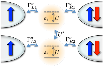
Figure 1: Schematic of a double quantum dot (DQD) system with ferromagnetic leads. Each dot, with energy level $\varepsilon_{j}$ and Coulomb correlation $U$, is coupled to a pair of left and right leads with coupling strength $\Gamma_{rj}^{\sigma}$. The Coulomb correlations between the dots are denoted by $U^{\prime}$. The magnetizations of the leads are assumed to form either a parallel (P) or antiparallel (AP) magnetic configuration.

The setup we consider consists of two capacitively coupled quantum dots, each one coupled to external leads (see the sketch in Fig. 1). Each dot is described by the single impurity Anderson model (SIAM). We denote by $\varepsilon_{j}$, with $j=\{1,2\}$, the energy of an electron residing in dot $j$. Each dot can accommodate up to two electrons, and they interact with each other through an on-site interaction $U$ and an interdot interaction $U^{\prime}$. Their occupation is denoted by $n_{j\sigma}=d^{\dagger}_{j\sigma}d_{j\sigma}$, with $d^{\dagger}_{j\sigma}$ creating a spin-$\sigma$ electron in dot $j$. The double dot Hamiltonian then reads

$$H_{\rm DQD} = \sum_{j\sigma}\varepsilon_{j}n_{j\sigma}+\sum_{j}Un_{j\uparrow}n_{j\downarrow}$$ (1)

$$+ U^{\prime}(n_{1\uparrow}+n_{1\downarrow})(n_{2\uparrow}+n_{2\downarrow})\,.$$

In the absence of an external magnetic field, $B=0$, if the energy levels are degenerate, i.e. $\varepsilon_{1}=\varepsilon_{2}$, and when $U=U^{\prime}$, the $H_{\rm DQD}$ Hamiltonian is $SU(4)$ invariant Nishikawa et al. (2013b); fn (1). When the orbital degeneracy is lifted, corresponding to a situation when $\varepsilon_{1}\neq\varepsilon_{2}$, $H_{\rm DQD}$ remains $SU(2)$ invariant in the spin sector. For more realistic situations Keller et al. (2014), when $U^{\prime}/U<1$, the $SU(4)$ symmetry is in general lost. Still, in this case, the system exhibits a special point in the $\{\varepsilon_{1},\varepsilon_{2}\}$ parameter space where an emergent $SU(4)$ symmetry can occur Nishikawa et al. (2013b), i.e. $\{\varepsilon_{1},\varepsilon_{2}\}\approx\{-U^{\prime}/2,-U^{\prime}/2\}$ fn (2). This special point will be discussed in more detail in Secs. III and V. The double dot setup is attached to four external ferromagnetic leads, modeled as reservoirs of noninteracting quasiparticles,

$$H_{\rm Leads}=\sum_{rj{\bf k}\sigma}\varepsilon_{rj{\bf k}\sigma}c^{\dagger}_{rj{\bf k}\sigma}c_{rj{\bf k}\sigma}\,.$$ (2)

Here, $c^{\dagger}_{rj{\bf k}\sigma}$ is the creation operator for an electron with momentum ${\bf k}$ and spin $\sigma$ in the lead $r=\{L,R\}$ attached to dot $j$. Consequently, the corresponding local density of states $\rho_{rj}^{\sigma}$ becomes spin dependent. Furthermore, this affects the broadening function that describes the coupling between the dots and the leads, i.e. $\Gamma_{rj}^{\sigma}=\pi\rho_{rj}^{\sigma}|v_{rj}|^{2}$, where $v_{rj}$ is the amplitude of the tunneling. The tunneling Hamiltonian is given by

$$H_{\rm Tun}=\sum_{rj{\bf k}\sigma}v_{rj}\left(c^{\dagger}_{rj{\bf k}\sigma}d_{j\sigma}+d^{\dagger}_{j\sigma}c_{rj{\bf k}\sigma}\right).$$ (3)

It is more convenient to express the couplings in terms of spin polarization of a given lead, $p_{rj}$, as $\Gamma_{rj}^{\sigma}=(1+\sigma p_{rj})\Gamma_{rj}$, where $\Gamma_{rj}=(\Gamma_{rj}^{\uparrow}+\Gamma_{rj}^{\downarrow})/2$. In the present work, we assume that the magnetizations of the leads are collinear and can take two configurations: ($i$) parallel (P) and ($ii$) antiparallel (AP). We also consider that the density of states is flat with the bandwidth given by $2D$, and set $D\equiv 1$ as the energy unit. The total Hamiltonian describing the double dot system coupled to ferromagnetic leads is then given by

$$H=H_{\rm DQD}+H_{\rm Leads}+H_{\rm Tun}.$$ (4)

In the following we will solve it using the Wilson’s NRG method Wilson (1975).

III The $SU(4)$ to $SU(2)$ crossover in the Kondo regime

We shall first focus on the special point $\{\varepsilon_{1},\varepsilon_{2}\}=\{-U^{\prime}/2,U^{\prime}/2\}$ that displays the emerging $SU(4)$ physics (provided $U\gtrsim U^{\prime}$ Nishikawa et al. (2013b)) in the limit when the leads are nonmagnetic. For finite spin polarization of the leads, the spin degeneracy is lifted, but the orbital $SU(2)$ symmetry is preserved. So, by changing the polarization of the external leads, it is possible to capture the $SU(4)\to SU(2)$ crossover. To comprehend the essential physics we map the Hamiltonian (4) to the Kondo model by projecting onto the subspace with single occupancy $\langle n\rangle\simeq 1$ by using the Schrieffer-Wolff transformation hew . We assume that the dots are symmetrically coupled, $v_{Lj}=v_{Rj}=v_{j}$ and $p_{Lj}=p_{Rj}=p$. We then make a change of basis by performing a unitary transformation on the leads operators and use an even/odd combination,

$$\left(\begin{array}[]{cc}c_{ej\bf k\sigma}\\ c_{oj\bf k\sigma}\end{array}\right) = \frac{1}{\sqrt{2}}\left(\begin{array}[]{cc}1&1\\ -1&1\end{array}\right)\left(\begin{array}[]{cc}c_{Lj\bf k\sigma}\\ c_{Rj\bf k\sigma}\end{array}\right)\;.$$ (11)

In this even-odd basis, the odd channel becomes decoupled and the double-dot remains coupled only to the even channel. In what follows, we shall drop the corresponding subscript, i.e., $c_{ej\bf k\sigma}\to c_{j\bf k\sigma}$. We introduce the tensor product notations $(\hat{\sigma}^{\mu}\otimes\hat{\tau}^{\nu})_{j\sigma;j^{\prime}\sigma^{\prime}}=\sum_{\textbf{kk}^{\prime}}c_{j\textbf{k}\sigma}^{\dagger}\sigma^{\mu}_{\sigma\sigma^{\prime}}\tau^{\nu}_{jj^{\prime}}c_{j^{\prime}\textbf{k}^{\prime}\sigma^{\prime}}$ and $(\hat{S}^{\mu}\otimes\hat{T}^{\nu})_{j\sigma;j^{\prime}\sigma^{\prime}}=d_{j\sigma}^{\dagger}\,(\frac{1}{2}\sigma^{\mu}_{\sigma\sigma^{\prime}})(\frac{1}{2}\tau^{\nu}_{jj^{\prime}})\,d_{j^{\prime}\sigma^{\prime}}$, where $\sigma^{\mu}=\{I_{2},\sigma_{x},\sigma_{y},\sigma_{z}\}$ are the regular Pauli matrices for $\mu=1\to 3$ and the unit matrix when $\mu=0$, acting in the spin degrees of freedom, and similar for $\tau^{\nu}$ but acting on the orbital part. Then, disregarding the potential scattering, the anisotropic Kondo Hamiltonian can be written as

$$H_{\mathrm{K}}=\sum_{\begin{subarray}{c}\sigma\sigma^{\prime}\alpha\alpha^{\prime}\\ jj^{\prime}ii^{\prime}\\ \mu\nu\end{subarray}}J^{\mu;\nu}_{j\sigma;j^{\prime}\sigma^{\prime}}(\hat{\sigma}^{\mu}\otimes\hat{\tau}^{\nu})_{j\sigma;j^{\prime}\sigma^{\prime}}(\hat{S}^{\mu}\otimes\hat{T}^{\nu})_{i\alpha;i^{\prime}\alpha^{\prime}}\;.$$ (12)

Altogether there are 15 terms in Eq. (12) and the exchange couplings $J^{\mu;\nu}_{j\sigma;j^{\prime}\sigma^{\prime}}$ depend on all the parameters of the original Hamiltonian, i.e. $\varepsilon_{j},U$ and $\Gamma_{rj}^{\sigma}$. In the limiting case when $U=U^{\prime}$ and $p=0$, it is straightforward to show that all the couplings are equal $\mathbf{J}\to J$ and the charge and spin contributions combine in an $SU(4)$-symmetric way. The $15=4^{2}-1$ generators for the $SU(4)$ Lie algebra are $\{I_{2},\bm{\sigma}\}\otimes\{I_{2},\bm{\tau}\}-I_{2}\otimes I_{2}$. On the other hand, when $p=1$, i.e. the leads are frozen for example in the spin-$\uparrow$ state, $H_{\rm K}$ remains $SU(2)$ invariant in the orbital sector.

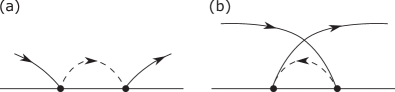
Figure 2: Second order diagrams contributing to the renormalization of the coupling matrix displaying processes when a virtual particle is scattered in the upper band edge (a) or a virtual hole in the lower band edge (b) of the lead electrons.

To capture the crossover we performed the RG analysis hew for the exchange couplings $\mathbf{J}$ in between these two fixed points. The second-order processes (particle and hole-like) that renormalize the couplings are displayed in Fig. 2. Keeping in mind that the polarization of the leads affects only the spin sector, we can group the couplings into $5$ distinct classes. Furthermore, we define dimensionless couplings by introducing the local density of states $\rho_{0}=1/2D_{0}$ as

$$j_{1}= \rho_{0}J^{\mu=\{0,3\};\nu\neq 0}_{j\uparrow;j^{\prime}\uparrow}\;, j_{2}=\rho_{0}J^{\mu=\{0,3\};\nu\neq 0}_{j\downarrow;j^{\prime}\downarrow},$$

$$j_{3}= \rho_{0}J^{\mu=\{1,2\};\nu}_{j\sigma;j^{\prime}\overline{\sigma}}\;, j_{4}=\rho_{0}J^{3;0}_{j\uparrow;j\uparrow}\,,$$

$$j_{5}=\rho_{0}J^{3;0}_{j\downarrow;j\downarrow}\,,$$

subject to initial conditions $j^{0}_{1}=j^{0}_{4}=\rho_{0}J^{0}(1+p),j^{0}_{2}=j^{0}_{5}=\rho_{0}J^{0}(1-p)$ and $j^{0}_{3}=\rho_{0}J^{0}\sqrt{1-p^{2}}$, where $J^{0}=v^{2}\left(\frac{1}{\varepsilon+U}-\frac{1}{\varepsilon}\right)$ and $v$ is the isotropic coupling fn (3). Here $2D_{0}$ is the bandwith for the conduction electrons. To second order in $\mathbf{j}$, the scaling equations are easily derived by progressively reducing the bandwidth $D$ hew as

$$\frac{dj_{1}}{d\ln D}=-2j_{3}^{2}-2j_{1}^{2}\;$$

$$\frac{dj_{2}}{d\ln D}=-2j_{3}^{2}-2j_{2}^{2}\;$$

$$\frac{dj_{3}}{d\ln D}=-\frac{3}{2}j_{3}(j_{1}+j_{2})-\frac{1}{2}j_{3}(j_{4}+j_{5})\;$$ (14)

$$\frac{dj_{4}}{d\ln D}=-4j_{3}^{2}\;$$

$$\frac{dj_{5}}{d\ln D}=-4j_{3}^{2}\;.$$

The $SU(4)$ fixed point is captured by setting $p=0$, in which case the set (III) of equations collapses to a single one, i.e. $dj/d\ln D=-4j^{2}$. In contrast, when the leads are fully polarized, $p=1$, the coupling $j_{4}$ remains marginal while $j_{1}$ rescales accordingly to the regular $SU(2)$ Kondo physics, $dj_{1}/d\ln D=-2j_{1}^{2}$. In the general situation we can solve the RG equations (III) numerically. A typical solution is presented in Fig. 3(a) for $p=0.8$, and as expected all the couplings diverge at the same characteristic energy scale that can be associated with the Kondo temperature hew .

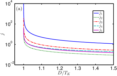
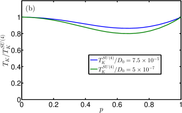
Figure 3: (a) The renormalization of the coupling constants as the bandwidth is changed. We used $p=0.8$ and $\rho_{0}J^{0}=0.026$. For this choice of parameters, $T_{K}/D_{0}=6.6\times 10^{-5}$. (b) The evolution of $T_{K}$ as a function of spin polarization $p$.

In general, in the $SU(N)$ Kondo model hew , apart from some higher-order corrections Filippone et al. (2014), the Kondo temperature is $T_{K}^{SU(N)}\simeq D_{0}\,e^{-1/(Nj_{0})}$. On the other hand, when the polarization of the leads is changed from $p=0\to 1$, we double the exchange interaction, so that $T_{K}$ is expected to remain unchanged. To test this conjecture, we represent in Fig. 3(b) the evolution of $T_{K}$ with the spin polarization $p$ of the leads, which indeed shows that $T_{K}$ is the same at the two fixed points. When $U\gg U^{\prime}$, depending on the ratios $\Gamma/U$ and $\Gamma/U^{\prime}$, the two characteristic energy scales, $T_{K}^{SU(2)}$ and $T_{K}^{SU(4)}$, can be well separated, but otherwise the physics remains the same.

To conclude this section, the set (III) of RG equations describes consistently the $SU(4)\to SU(2)$ crossover and captures the essential Kondo physics in between the two fixed points. In Sec. V, we supplement the RG analysis with more exact numerical renormalization group calculations Wilson (1975); Fle and focus on computing measurable quantities such as the conductance and the tunnel magnetoresistance.

IV Numerical renormalization group and the conductance

In this work we are interested in the linear response transport properties of the system at low enough temperatures such that the electron correlations give rise to the Kondo effect Kondo (1964); hew . The aim, in particular, is to elucidate the role of spin-dependent tunneling on the transport properties in the full parameter space, with a special focus on the $SU(4)$ Kondo regime Borda et al. (2003). In order to achieve this goal in the most accurate manner, we employ the nonperturbative numerical renormalization group (NRG) method Wilson (1975); Fle . In the NRG approach, the conduction bands of the non-interacting electrons in the leads are discretized in a logarithmic way with a discretization parameter $\Lambda$ (here we use $\Lambda=2$). The discretized Hamiltonian is then transformed to a tight-binding chain Hamiltonian with exponentially decaying hoppings (Wilson chain).

We follow the same strategy as discussed in Sec. III and use the even-odd basis. In this way each dot is coupled to a single channel – the even channel – with a coupling strength, $\Gamma_{j}^{\sigma}=\Gamma_{Lj}^{\sigma}+\Gamma_{Rj}^{\sigma}$. The NRG Hamiltonian of the system is

$$H_{\rm NRG} = H_{\rm DQD}+\sum_{j\sigma}\sqrt{\frac{\Gamma_{j}^{\sigma}}{\rho_{0}\pi}}\left(f_{j0\sigma}^{\dagger}d_{j\sigma}+d_{j\sigma}^{\dagger}f_{j0\sigma}\right)$$ (15)

$$+ \sum_{jn\sigma}\xi_{n}\left(f^{\dagger}_{jn\sigma}f_{jn+1\sigma}+f_{jn+1\sigma}^{\dagger}f_{jn\sigma}\right).$$

Here, $f^{\dagger}_{jn\sigma}$ denotes the creation operator of a spin-$\sigma$ electron at site $n$ ($n=0,1,2\dots$) of the $j^{\rm th}$ ($j=1,2$) Wilson chain and $\xi_{n}$ are the respective hopping integrals. This Hamiltonian is solved iteratively by retaining an appropriate number $N_{K}$ of low-energy states at each iteration (here we keep at least $N_{K}=10^{4}$ states). The discarded states, on the other hand, form a complete many-body basis of the whole NRG Hamiltonian Anders and Schiller (2005) and are used to construct the full density matrix of the system Weichselbaum and von Delft (2007).

Along the NRG procedure, one needs to deal with a large Hilbert space at each step of iteration, therefore it is crucial to exploit as many symmetries of the NRG Hamiltonian as possible. Here we make use of four Abelian symmetries fn (4), defined by the generators

$$Q_{j} = \sum_{\sigma}\left(n_{j\sigma}-\tfrac{1}{2}\right)+\sum_{n\sigma}\left(f_{jn\sigma}^{\dagger}f_{jn\sigma}-\tfrac{1}{2}\right),$$ (16)

$$S_{z}^{j} = \frac{1}{2}\left(n_{j\uparrow}-n_{j\downarrow}\right)+\frac{1}{2}\sum_{n}\left(f_{jn\uparrow}^{\dagger}f_{jn\uparrow}-f_{jn\downarrow}^{\dagger}f_{jn\downarrow}\right),$$

for the total charge and $z^{\rm th}$ spin component of dot and chain $j$, respectively. The quantities we are particularly interested in are $(i)$ the total spectral function

$$A(\omega)=\sum_{j\sigma}A_{j\sigma}(\omega)=-\frac{1}{\pi}\sum_{j\sigma}{\rm Im}G_{j\sigma}^{R}(\omega),$$ (17)

with $G_{j\sigma}^{R}(\omega)$ being the Fourier transform of the retarded Green’s function, $G_{j\sigma}^{R}(t)=-i\Theta(t)\langle\{d_{j\sigma}(t),d_{j\sigma}^{\dagger}(0)\}\rangle$, and $(ii)$ the linear conductance

$$G=\frac{e^{2}}{h}\sum_{j\sigma}\frac{4\Gamma_{Lj}^{\sigma}\Gamma_{Rj}^{\sigma}}{\Gamma_{Lj}^{\sigma}+\Gamma_{Rj}^{\sigma}}\int\!\!d\omega\left(\!\!-\frac{\partial f(\omega)}{\partial\omega}\right)\pi A_{j\sigma}(\omega),$$ (18)

where $f(\omega)$ denotes the Fermi-Dirac distribution function fn (5); Meir and Wingreen (1992). To get a clear picture, we assume equal spin polarizations of the leads, $p_{rj}\equiv p$, and equal coupling strengths, $\Gamma_{rj}\equiv\Gamma/2$. Then the expression (18) for the linear conductance reduces to

$$G^{\rm AP}=\frac{2e^{2}}{h}(1-p^{2})\Gamma\int\!\!d\omega\left(\!\!-\frac{\partial f(\omega)}{\partial\omega}\right)\pi A^{\rm AP}(\omega),$$ (19)

for the antiparallel (AP) configuration, with $A_{j}^{\rm AP}(\omega)=A_{j\uparrow}^{\rm AP}(\omega)=A_{j\downarrow}^{\rm AP}(\omega)$ the spectral function in the AP configuration. As can be seen, $G^{\rm AP}$ is the linear conductance – up to the prefactor $(1-p^{2})$ – of a DQD setup with nonmagnetic leads. On the other hand, the conductance in the parallel (P) configuration is given by

$$G^{\rm P}=\frac{e^{2}}{h}\sum_{\sigma}(1+\sigma p)\Gamma\int\!\!d\omega\left(\!\!-\frac{\partial f(\omega)}{\partial\omega}\right)\pi A_{\sigma}^{\rm P}(\omega),$$ (20)

where $A_{j\sigma}^{\rm P}(\omega)$ is the spectral function in the parallel configuration. The difference between the conductances in both magnetic alignments can be described by the tunnel magnetoresistance, which is defined as, Julliere (1975); Barnaś and Weymann (2008) ${\rm TMR}=G^{\rm P}/G^{\rm AP}-1$. In the present work we use the NRG to investigate the full phase space of the model. However, to connect to the RG results presented in Sec. III, let us first discuss the $SU(4)\to SU(2)$ crossover and follow the evolution of the spectral functions as well as of the conductance, quantities that were not accessible in the RG approach.

V The $SU(4)$ to $SU(2)$ crossover: NRG results

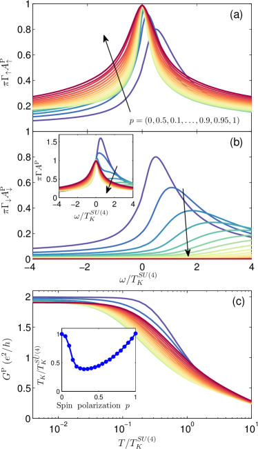
Figure 4: The energy dependence of (a) the zero-temperature spin-up and (b) spin-down spectral function, together with (c) the linear conductance as a function of temperature calculated for different spin polarization of the leads, ranging from $p=0$ to $p=1$ in steps of 0.05 (the arrow indicates the direction in which $p$ increases), in the $SU(4)$ Kondo regime. The inset in (b) shows the total spectral function, while the inset in (c) presents the Kondo temperature as a function of $p$. The Kondo temperature is defined by $G(T)/G(T=0)=1/2$. $T_{K}^{SU(4)}$ ($\approx 2.8\cdot 10^{-4}U$) denotes the $SU(4)$ Kondo temperature (in the case of $p=0$). The parameters are: $U=U^{\prime}=0.5$, $\Gamma=0.015$, in units of band halfwidth, and $\varepsilon_{1}=\varepsilon_{2}=-U^{\prime}/2$.

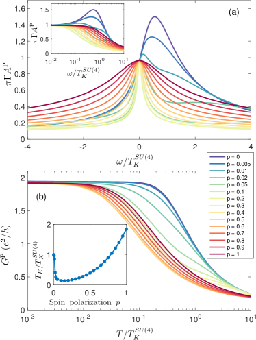
Figure 5: (a) The energy dependence of the zero-temperature total spectral function, and (b) the temperature dependence of the linear conductance calculated for different spin polarization of the leads, as indicated. The inset in (a) shows the spectral function on the logarithmic scale, while the inset in (b) presents the Kondo temperature as a function of $p$. The parameters are the same as in Fig. 4 with $U=1$ and $U^{\prime}=U/2$. Now $T_{K}^{SU(4)}/U\approx 7.5\cdot 10^{-5}$.

In this section we focus on the $SU(4)$ Kondo regime and analyze the influence of finite leads’ spin polarization on the transport properties. We shall present the results for the spectral functions $A_{\sigma}^{\rm P}(\omega)$ as well as for the temperature dependence of the conductance fn (6). We will discuss in detail the case of $U=U^{\prime}$, and later address a more realistic situation when $U>U^{\prime}$.

An important quantity that captures the crossover is the normalized spectral function, $A_{\sigma}^{\rm P}(\omega)$, whose spin components are displayed in Figs. 4(a) and (b), respectively. The total spectral function itself, $A^{\rm P}(\omega)$, is presented in the inset of Fig. 4(b). When $p=0$, it displays the regular $SU(4)$ Kondo resonance formed away from the Fermi level at $\omega\approx T_{K}^{SU(4)}$. When increasing the spin polarization its maximum becomes suppressed and moves toward $\omega=0$, and when $p=1$ the orbital-$SU(2)$ Kondo resonance is formed at $\omega=0$.

We can get more information by inspecting the spin-resolved spectral functions. In the case of spin-up channel, which belongs to the majority-spin subband, increasing the spin polarization results in an enhancement of the spectral function to $A_{\uparrow}^{\rm P}(\omega\to 0)\simeq 1/\pi\Gamma_{\uparrow}$. Moreover, the maximum in $A_{\uparrow}^{\rm P}(\omega)$ gradually shifts to the Fermi energy, such that for $p=1$, only the orbital degree of freedom is relevant, and the $SU(2)$ Kondo peak becomes symmetric around $\omega=0$. On the other hand, $A_{\downarrow}^{\rm P}(\omega)$ exhibits a completely different behavior. First of all, increasing the spin polarization results in a decrease of $A_{\downarrow}^{\rm P}(\omega)$. Furthermore, the maximum in the spin-down spectral function moves away from the Fermi energy, due to the development of the exchange field $\Delta\varepsilon_{\rm exch}$ Martinek et al. (2003a, b) and this splitting grows with increasing $p$. Finally, for $p=1$, $A_{\downarrow}^{\rm P}(\omega)$ becomes completely quenched at low energies.

This distinct behavior of the spectral function is corroborated with a detailed analysis of the temperature dependence of the linear conductance, which is shown in Fig. 4(c). At the two fixed points (corresponding to $p=0$ and $p=1$), the conductance is a universal function of $T/T_{K}^{SU(N)}$ Borda et al. (2003); Keller et al. (2014).

Interestingly, despite the fact that the system’s ground state degeneracy becomes reduced from four-fold to two-fold, increasing the spin polarization has a rather small effect on the conductance itself. Its temperature dependence allows us to define the Kondo scale as $G^{\rm P}(T=T_{K})=G^{\rm P}(T=0)/2$. The evolution of $T_{K}$ with increasing the spin polarization is presented in the inset of Fig. 4(c). As previously predicted by the RG equations, the polarization of the leads has a relatively small effect on $T_{K}$ and, consequently, $T_{K}^{SU(4)}\approx T_{K}^{SU(2)}$. We would however like to note that the difference between the two Kondo temperatures can be enlarged by reducing the charge fluctuations, i.e. by decreasing the ratio of $\Gamma/U$.

Let us now analyze a more realistic situation when $U>U^{\prime}$. Now the two Kondo temperatures $T_{K}^{SU(N=2,4)}$ are well separated, which allows us to clearly identify the exchange-field-induced splitting in the conductance behavior. This can be obtained by properly tuning the ratio between the couplings and Coulomb correlations. The energy dependence of the spectral function and the temperature dependence of the conductance calculated for $\Gamma/U=0.015$ are shown in Fig. 5. Since $T_{K}^{SU(4)}$ is now much smaller ($T_{K}^{SU(4)}/U\approx 7.5\cdot 10^{-5}$), a very small spin polarization ($p\gtrsim 0.02$) is sufficient to suppress the $SU(4)$ Kondo effect completely [see Fig. 5(a)]. Quite unexpectedly, the width of the orbital Kondo peak depends in a nonmonotonic fashion on the degree of spin polarization of the leads [see also the inset in Fig. 5(a)], and the minimum width occurs around $p\approx 0.1$.

This behavior is now clearly reflected in the temperature dependence of the conductance shown in Fig. 5(b). The $p=0$ curve presents a universal $SU(4)$ conductance dependence, which then, with increasing $p$, smoothly changes to the $SU(2)$ universal curve. Moreover, the extracted Kondo temperature reveals a nonmonotonic dependence on spin polarization. First, the Kondo temperature quickly drops with $p$ and is much lower than $T_{K}^{SU(4)}$. Further increase of $p$, however, results in an enhancement of the $SU(2)$ Kondo temperature. To understand this enhancement, we recall that spin-dependent hybridization (which grows with $p$), results in DQD level renormalization, such that the position of the spin-up levels becomes effectively lowered. As a consequence, it reduces the excitation energies for the pseudo-spin-flip processes responsible for the Kondo effect, leading to an increase of $T_{K}^{SU(2)}$, such that for $p=1$, one may even achieve $T_{K}^{SU(2)}>T_{K}^{SU(4)}$, see the inset of Fig. 5(b), which is not in general obvious.

VI Stability diagrams and tunnel magnetoresistance

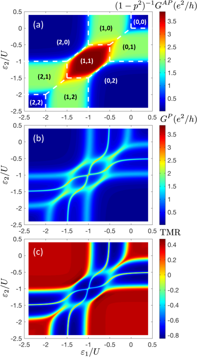
Figure 6: The linear conductance in (a) the antiparallel and (b) parallel magnetic configuration and (c) the resulting TMR as a function of DQD energy levels $\varepsilon_{1}$ and $\varepsilon_{2}$. The dashed lines in (a) mark the regions where the DQD is in a state ($n_{1}$,$n_{2}$) with $n_{1}$ ($n_{2}$) electrons in first (second) dot. The parameters are: $U=1$, $U^{\prime}=0.5$, $\Gamma=0.07$, $p=0.4$ and $T=10^{-6}$.

In this section we present results for the low-temperature linear conductance in the parallel and antiparallel configurations, together with the TMR, calculated as a function of the double dot energy levels $\varepsilon_{1}$ and $\varepsilon_{2}$. In Fig. 6 we present a typical stability diagram that covers the full parameter space, from empty to fully occupied DQD. In this section we address only the regime where $U/U^{\prime}=2$.

Let us first discuss the case of the antiparallel magnetic configuration shown in Fig. 6(a). The conductance shows a pattern that closely resembles that of nonmagnetic DQD system Kouwenhoven et al. (1997). The dashed lines separate the equilibrium charged transport domains. When the number of electrons in each dot is even, the DQD is in a singlet state, no Kondo effect develops and the observed low conductance results only from cotunneling processes. However, when the electron number in either quantum dot is odd, the electronic correlations can give rise to an enhanced conductance due to the Kondo effect, provided the temperature is lower than the Kondo temperature. In our calculations the assumed temperature is very low, $T\simeq 10^{-6}U$, such that in each Coulomb blockade region the Kondo effect develops.

As the parameter space is relative large, depending on the nature of the ground state, several types of the Kondo effects develop. When the occupancy of one of the dots is odd, a typical spin-$SU(2)$ Kondo effect develops. This can be observed in transport regime with the electron numbers belonging to the set $\{(1,0),(0,1),(2,1),(1,2)\}$ [see Fig. 6(a)], where $G^{\rm AP}/(1-p^{2})$ reaches the unitary limit $\approx 2e^{2}/h$. Since there is no direct hopping between the dots, when every dot is singly occupied, $(n_{1},n_{2})=(1,1)$ one finds that the $SU(2)$ Kondo effect develops independently in each quantum dot, such that the total conductance reaches $G^{\rm AP}/(1-p^{2})\approx 4e^{2}/h$.

The stability diagram allows us to get a better understanding of how the emergent $SU(4)$ Kondo effect develops: along the line separating the charge states $(0,1)\leftrightarrow(1,0)$, and $(2,1)\leftrightarrow(1,2)$, besides the spin degeneracy an additional orbital degeneracy is present and the ground state is four-fold degenerate. Consequently, the system exhibits the $SU(4)$ Kondo effect Keller et al. (2014). As we have seen in Sec. V, the $SU(4)$ Kondo state is better revealed in the parallel configuration, where the spin degeneracy is broken.

The conductance in the parallel configuration is presented in Fig. 6(b) and reveals some huge differences when compared to the AP configuration. This is due to the emergence of the exchange field $\Delta\varepsilon_{\rm exch}$ that splits the levels of the DQD and lifts the spin degeneracy Wójcik (2015). As a consequence, since the orbital degeneracy is not affected, one observes the orbital-$SU(2)$ Kondo effect along the lines separating the charge states with occupation $(0,1)\leftrightarrow(1,0)$, and $(1,2)\leftrightarrow(2,1)$ electrons, as well as $(2,0)\leftrightarrow(1,1)$ and $(1,1)\leftrightarrow(0,2)$, see Fig. 6(b). Otherwise the conductance is generally suppressed except for some special lines where $\Delta\varepsilon_{\rm exch}\approx 0$.

For a single quantum dot Martinek et al. (2005b), $\Delta\varepsilon_{\rm exch}\approx(2p\Gamma/\pi)\log|\varepsilon/(\varepsilon+U)|$ and vanishes, i.e. $\Delta\varepsilon_{\rm exch}\approx 0$, at the particle-hole symmetry point $\varepsilon=-U/2$. In the absence of coupling between the two dots, the Kondo effect in the first (second) dot would be thus present for $\varepsilon_{1}=-U/2$ ($\varepsilon_{2}=-U/2$) for any value of $\varepsilon_{2}$ ($\varepsilon_{1}$), resulting in straight vertical and horizontal lines in the $(\varepsilon_{1},\varepsilon_{2})$-plane of the Kondo-enhanced conductance. However, in the presence of capacitive coupling between the dots, the lines become distorted by the inter-dot Coulomb correlations $U^{\prime}$, as can be seen in Fig. 6(b).

The difference in conductance in the two magnetic configurations is reflected in the TMR, which is shown in Fig. 6(c). For transport regimes with even occupancy of each dot, elastic cotunneling processes dominate the current and the TMR is given by Weymann et al. (2005) ${\rm TMR}\approx 2p^{2}/(1-p^{2})$. For odd occupancy, the Kondo effect is present in the case of antiparallel configuration, while in the parallel configuration it is suppressed by the exchange field, such that $G^{\rm P}\ll G^{\rm AP}$ and ${\rm TMR}\to-1$ Weymann (2011). On the other hand, for such values of $\varepsilon_{1}$ and $\varepsilon_{2}$ that the exchange field vanishes, one has, $G^{\rm AP}/G^{\rm P}=1-p^{2}$, which yields ${\rm TMR}=p^{2}/(1-p^{2})$, a ratio which is valid irrespective of the $SU(2)$ or $SU(4)$ Kondo regimes.

To understand the influence of ferromagnetic leads on transport, in the following we will analyze the behavior of the conductance and the TMR as function of spin polarization of the leads, as well as temperature along different cuts in the stability diagram. We shall consider two such cross-sections defined as: $(i)$ $\varepsilon_{2}+\varepsilon_{1}=-U^{\prime}$ and $(ii)$ $\varepsilon_{1}=\varepsilon_{2}$, in the stability diagram. In what follows we shall label them cut (line) 1 and 2.

VI.1 Conductance and TMR along cross-sections

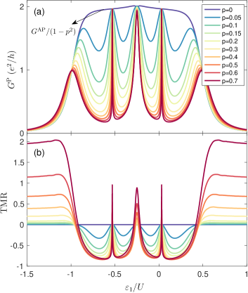
Figure 7: (a) The linear conductance in both magnetic configurations and (b) the resulting TMR as a function of $\varepsilon_{1}$ with $\varepsilon_{2}=-\varepsilon_{1}-U^{\prime}$ calculated for different values of leads’ spin polarization $p$, as indicated. The conductance in the antiparallel configuration is given by the curve for $p=0$ multiplied with a factor of $(1-p^{2})$, cf. Eq. (19). The parameters are the same as in Fig. 6.

The linear conductance in both magnetic configurations and the TMR calculated as a function of $\varepsilon_{1}$ with $\varepsilon_{2}+\varepsilon_{1}=-U^{\prime}$ for different values of spin polarization $p$ are shown in Fig. 7. By changing the level position, the occupation of the DQD changes from $(2,0)$ for $\varepsilon_{1}\lesssim-U$, to $(1,0)$ for $-U\lesssim\varepsilon_{1}\lesssim-U^{\prime}/2$, $(0,1)$ for $-U^{\prime}/2\lesssim\varepsilon_{1}\lesssim U/2$, and to ($0,2$) for $\varepsilon_{1}\gtrsim U/2$. In the nonmagnetic lead case, in the odd occupancy regime the regular spin-$SU(2)$ Kondo effect develops with conductance reaching $\approx 2e^{2}/h$, see Fig. 7(a). Moreover, for $\varepsilon_{1}=-U^{\prime}/2$, an additional orbital degeneracy occurs and the system exhibits the $SU(4)$ Kondo effect, but the conductance remains $G\approx 2e^{2}/h$. These different types of the Kondo effects are hardly distinguishable by the conductance itself when $T\ll\{T_{K}^{SU(2)},T_{K}^{SU(4)}\}$, as it remains close to the unitary value, $G\approx 2e^{2}/h$ in the whole singly occupied DQD regime, see Fig. 7(a). However, they can be revealed at larger temperatures, i.e. $T\gtrsim\{T_{K}^{SU(2)},T_{K}^{SU(4)}\}$ or in the case of ferromagnetic leads.

When $p>0$, the conductance gets modified. The behavior in the AP configuration is still featureless, similar to the case of normal leads as $G^{\rm AP}(p)=G^{\rm AP}(p=0)(1-p^{2})$. However, the conductance in the P configuration reveals a nontrivial interplay between the spin-resolved DQD level renormalization and the correlations bringing about the Kondo effect. With increasing the spin polarization, the strength of the exchange field increases and once $|\Delta\varepsilon_{\rm exch}|$ becomes larger than the corresponding Kondo scale, the conductance drops. This can be observed in the whole odd occupation regime shown in Fig. 7, i.e. for $-U\lesssim\varepsilon_{1}\lesssim U/2$, except for some special values of the level position where, again, $\Delta\varepsilon_{\rm exch}\approx 0$. For $\varepsilon_{1}\approx-U/2$, the exchange field in the first dot vanishes, while for $\varepsilon_{1}=0$ (corresponding to $\varepsilon_{2}\approx-U/2$) the exchange field in the second dot vanishes. As a result, the total conductance reveals two peaks for $\varepsilon_{1}\approx\{-U/2,0\}$ with an almost unitary conductance $G^{\rm P}\approx 2e^{2}/h$. The height of these peaks remains almost constant, but their width depends on $p$, as the exchange field increases with $p$, and a smaller detuning is needed for the condition $|\Delta\varepsilon_{\rm exch}|\gtrsim T_{K}^{SU(2)}$ to be fulfilled. In addition, a spin-polarization independent resonance is also present for $\varepsilon_{1}=-U^{\prime}/2$ (note that then $\varepsilon_{2}=\varepsilon_{1}$). This is exactly the special point we have analyzed in Sec. III that shows the $SU(4)$ to $SU(2)$ crossover. Although the maximum value of conductance does not depend at this point on the polarization $p$, the system’s ground state does change. For $p=0$, it exhibits four-fold degeneracy, which becomes reduced to two-fold degeneracy when increasing spin polarization. Consequently, the $SU(4)$ Kondo effect becomes reduced to the orbital $SU(2)$ Kondo effect once $|\Delta\varepsilon_{\rm exch}|\gtrsim T_{K}^{SU(4)}$. The width of the resonance for $\varepsilon_{1}\approx-U^{\prime}/2$ is determined by the condition $|\Delta\varepsilon|\approx T_{K}^{SU(2)}$ fn (7), where $\Delta\varepsilon=\varepsilon_{2}-\varepsilon_{1}$ corresponds to the pseudo-Zeeman splitting.

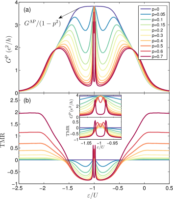
Figure 8: (a) The linear conductance in both magnetic configurations and (b) the resulting TMR as a function of $\varepsilon_{1}=\varepsilon_{2}\equiv\varepsilon$ calculated for different values of leads’ spin polarization $p$, as indicated. The inset shows the zoom into the transport regime around $\varepsilon=-U/2-U^{\prime}$. The conductance in the antiparallel configuration is given by the curve for $p=0$ multiplied with a factor of $(1-p^{2})$, cf. Eq. (19). The parameters are the same as in Fig. 6.

The $\varepsilon_{1}$-dependence of the TMR for different spin polarizations along the first cut we consider is shown in Fig. 7(b). The transport regimes discussed above are clearly visible. In the even occupation regime the TMR is given by ${\rm TMR}=2p^{2}/(1-p^{2})$, while in the case of odd DQD occupation, the TMR drops to ${\rm TMR}=-1$ with increasing $p$, except for $\varepsilon_{1}=-U/2$, $\varepsilon_{1}=-U^{\prime}/2$ and $\varepsilon_{1}=0$, where ${\rm TMR}=p^{2}/(1-p^{2})$.

Let us now analyze the transport behavior along the second cut, where $\varepsilon_{1}=\varepsilon_{2}\equiv\varepsilon$. Along this line, when $\varepsilon\gtrsim 0$, the DQD is empty, for $-U^{\prime}\lesssim\varepsilon\lesssim 0$ it is singly occupied, for $-U-U^{\prime}\lesssim\varepsilon\lesssim-U^{\prime}$ two electrons occupy the DQD, when $-2U\lesssim\varepsilon\lesssim-U-U^{\prime}$ there are three electrons in the DQD, while for $\varepsilon\lesssim-2U$ the DQD is fully occupied with four electrons. In the odd occupation regime, the ground state has four-fold degeneracy and the system exhibits the $SU(4)$ Kondo effect in the case of nonmagnetic leads. A plateau of $G\approx 2e^{2}/h$ associated with the $SU(4)$ Kondo effect is hardly visible as a function of $\varepsilon$, see the curve for $p=0$ in Fig. 8(a). This is because of a relatively large $\Gamma/U$ ratio considered in calculations and the usual spin $SU(2)$ Kondo effect, which develops in both quantum dots yielding $G=4e^{2}/h$ in the two-electron regime in the case of $p=0$. For finite $p$, in the parallel configuration the conductance becomes however suppressed, except for $\varepsilon\approx-U/2-U^{\prime}$, cf. Fig. 6(b), where the exchange field cancels and the Kondo phenomenon can develop. Moreover, the two plateaus in the odd-electron regime, associated with the orbital $SU(2)$ Kondo effect, are clearly visible, see e.g. the case of $p=0.7$ in Fig. 8(a). This confirms that for $p=0$, i.e. in the absence of level spin-splitting, the ground state of the system was indeed four-fold degenerate.

Another feature in the $\varepsilon$-dependence of the conductance can be seen around $\varepsilon=-U/2-U^{\prime}$ for finite $p$, see Fig. 8(a). As already mentioned, when $\varepsilon\approx-U/2-U^{\prime}$, the exchange field vanishes and one should observe the Kondo effect. However, instead of a peak at $\varepsilon\approx-U/2-U^{\prime}$, with increasing $p$, a dip develops with two small satellite peaks. This effect is associated with an interplay between finite temperature, exchange field and the Kondo temperature. First of all, one should note that exchange field can be tuned not only by changing the DQD levels (by inducing detuning from $\varepsilon=-U/2-U^{\prime}$), but it also grows with spin polarization Martinek et al. (2005b). Thus, for larger $p$, a smaller detuning from the point $\varepsilon=-U/2-U^{\prime}$ is needed to suppress the Kondo-enhanced conductance, see the width of $G^{P}$ in the inset in Fig. 8. On the other hand, increasing the spin polarization results in lowering of the corresponding Kondo temperature Martinek et al. (2003a) and, once $T_{K}\lesssim T$, the conductance becomes suppressed at $\varepsilon=-U/2-U^{\prime}$. The crucial observation is that $T_{K}$ also depends on detuning from the particle-hole symmetry point $\varepsilon=-U/2-U^{\prime}$ and grows with increasing this detuning. As a consequence, small side peaks, on either side of $\varepsilon=-U/2-U^{\prime}$, develop in $G^{P}$ for such values of $\varepsilon$ that $T_{K}\approx T$. Note that these peaks are visible as long as $T_{K}\gtrsim|\Delta\varepsilon_{\rm exch}|$, and once this condition is not met any more, which happens for even larger $p$, $G^{P}$ becomes suppressed.

The corresponding dependence of the TMR is shown in Fig. 8(b). In this figure one can clearly identify all the TMR values discussed earlier. In the empty and fully occupied DQD regime, the elastic cotunneling gives rise to ${\rm TMR}=2p^{2}/(1-p^{2})$. In the odd occupation regime, the TMR value drops by a factor of $2$, while in the case of $-U-U^{\prime}<\varepsilon<-U^{\prime}$ the TMR is generally suppressed by the exchange field, ${\rm TMR}\to-1$, except for the middle of the Coulomb diamond, i.e. around $\varepsilon=-U/2-U^{\prime}$. There, for large spin polarization, the TMR displays two peaks on either side of $\varepsilon=-U/2-U^{\prime}$, see the inset in Fig. 8(b), resulting from the corresponding peaks in $G^{P}$. The finite temperature effects visible in Fig. 8 lead our discussion to the analysis of transport properties at different temperatures. This is presented in the next section.

VI.2 Finite temperature effects

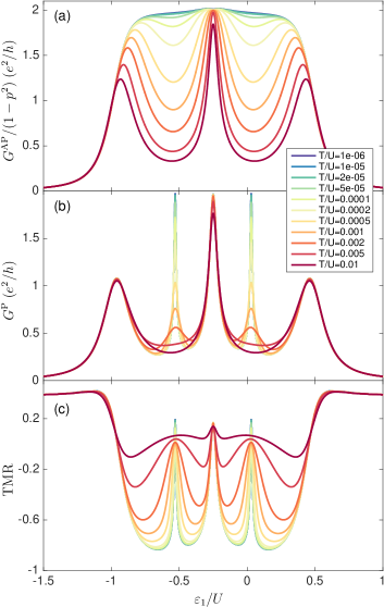
Figure 9: The linear conductance in (a) the antiparallel and (b) parallel magnetic configurations, as well as (c) the resulting TMR as a function of $\varepsilon_{1}$ with $\varepsilon_{2}=-\varepsilon_{1}-U^{\prime}$ calculated for different temperatures, as indicated. The other parameters are the same as in Fig. 6.

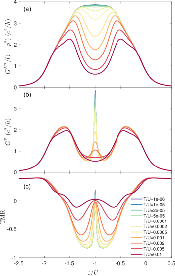
Figure 10: The linear conductance in (a) the antiparallel and (b) parallel magnetic configurations, as well as (c) the resulting TMR as a function of $\varepsilon_{1}=\varepsilon_{2}\equiv\varepsilon$ calculated for different temperatures, as indicated. The other parameters are the same as in Fig. 6.

In this section we discuss the effect of the temperature on the linear conductance and TMR. For that we evaluated the conductance in both AP and P magnetic configurations at various temperatures along the two cuts discussed in Sec. VI.1. In Fig. 9 we display the evolution of the conductance along the first cross-section, $\varepsilon_{1}$ with $\varepsilon_{2}+\varepsilon_{1}=-U^{\prime}$.

At low temperatures, i.e. $T\lesssim\{T^{SU(4)}_{K},T^{SU(2)}_{K}\}$, the conductance in the antiparallel configuration exhibits a plateau in the singly occupied DQD transport regime fn (8). This plateau changes when the temperature is increased. First, the conductance becomes suppressed in the $SU(2)$ Kondo regime, and at some intermediate temperature, $T^{SU(4)}_{K}\gtrsim T\gtrsim T^{SU(2)}_{K}$, the resonances at $\varepsilon_{1}\approx-U$ and $\varepsilon_{1}\approx U/2$ survive, together with the $SU(4)$ Kondo peak at $\varepsilon_{1}\approx-U^{\prime}/2$. From their temperature dependence one can also estimate the Kondo temperatures: In the middle of the spin $SU(2)$ Kondo valley and for parameters assumed in Fig. 9(a) one finds, $T_{K}^{SU(2)}/U\approx 8.96\cdot 10^{-4}$, while the $SU(4)$ Kondo temperature for $\varepsilon_{1}\approx-U^{\prime}/2$ is, $T_{K}^{SU(4)}/U\approx 0.044$.

On the other hand, the evolution of $G^{\rm P}(T)$ along the first cut is completely different: The Kondo plateau is not present at low temperatures, but only some narrow peaks occur at some specific values of $\varepsilon_{1}$. It is obvious that the ones occurring at $\varepsilon_{1}\approx-U/2$ and $\varepsilon_{1}\approx 0$ are associated with the spin-$SU(2)$ Kondo effect fn (9). Note that in the case of finite $p$, the Kondo temperature decreases with increasing spin polarization Martinek et al. (2003a). Although, based on the previous analysis, we can safely attribute the feature at $\varepsilon_{1}\approx-U^{\prime}/2$ to the $SU(4)$ Kondo effect, from the evolution of $G^{\rm P}$ itself it is not that straightforward to decide what type of correlations causes the conductance enhancement: If $|\Delta\varepsilon_{\rm exch}|\lesssim T_{K}^{SU(4)}$, then the $SU(4)$ nature of the ground state is relevant, whereas for $|\Delta\varepsilon_{\rm exch}|\gtrsim T_{K}^{SU(4)}$, the spin degeneracy is lifted and only the orbital degrees of freedom are degenerate, resulting in orbital Kondo effect. In fact, for parameters assumed in Fig. 9(b), the strength of the exchange field is comparable to $T_{K}^{SU(4)}$.

The effects of finite temperature on transport behavior along the second cut we considered ($\varepsilon_{1}=\varepsilon_{2}\equiv\varepsilon$) are presented in Fig. 10. In the case of antiparallel configuration, the conductance in the middle Coulomb blockade regime becomes quickly suppressed with increasing temperature. However, in the $SU(4)$ Kondo regime, the dependence of $G$ on $T$ is weak in the considered temperature range, since even for the highest temperature considered $T\lesssim T_{K}^{SU(4)}$. A similar tendency can be observed in the case of parallel alignment. A strong temperature dependence is only revealed for the Kondo peak at $\varepsilon_{1}=-U/2-U^{\prime}$, while in the other transport regimes the linear conductance only weakly depends on $T$.

Finally, the TMR evaluated at various temperatures along the two cross-sections is shown in Figs. 9(c) and 10(c). In these figures one can clearly identify all the TMR values discussed earlier. The general conclusion is that with increasing the temperature, TMR extrema become suppressed, such that in the very high temperature limit ($T\gtrsim U$, not shown), the TMR would be independent of $\varepsilon_{1}$ and $\varepsilon_{2}$, i.e. ${\rm TMR}\approx p^{2}/(1-p^{2})$ Weymann (2011).

VI.3 Ferromagnets with different coercive fields

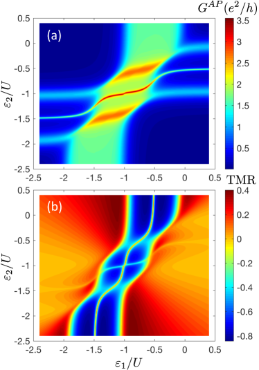
Figure 11: (a) The linear conductance in the mixed antiparallel configuration and (b) the TMR as a function of DQD energy levels. The parameters are same as in Fig. 6. In the mixed antiparallel configuration, the magnetization of one of the leads attached to the first dot is opposite to the other leads’ magnetizations.

In this section we discuss the magnetoresistive properties of the device assuming an experimentally relevant situation, when the coercive fields of the ferromagnetic electrodes are different. For sufficiently strong magnetic field (but still much smaller then the field necessary to induce a considerable Zeeman splitting), the magnetizations of all electrodes are aligned (parallel configuration). So far in our analysis we have assumed that there is a difference between coercive fields of the left and right electrodes, such that at certain field the leads on one side of the junction flip their magnetizations and the antiparallel configuration occurs, see Fig. 1. However, it may happen that only one of the electrodes flips its magnetic moment, resulting in a mixed antiparallel configuration: For example the leads coupled to the first dot are in the antiparallel, while the leads attached to the second one are in the parallel magnetic configuration. The transport characteristics for such a situation are shown in Fig. 11. One can still identify charged stability regions separated by lines with large conductance: When changing $\varepsilon_{1}$ the system exhibits a Kondo plateau (visible in the transport regions for $\varepsilon_{2}\lesssim-U-U^{\prime}$ and $\varepsilon_{2}\gtrsim-U^{\prime})$, while as a function of $\varepsilon_{2}$ the characteristic suppression of the Kondo resonance by the exchange field occurs, see Fig. 11(a). The total conductance shows then an enhancement to $G^{\rm AP}=4e^{2}(1-p^{2}/2)/h$ for such position of the DQD levels that the exchange field on the second dot vanishes. The whole DQD level dependence of conductance in the mixed configuration can be understood based on the analysis presented in Sec. VI.1, and it results in the associated behavior of the TMR, which is shown in Fig. 11(b).

VII Conclusions

In this paper we studied the linear-response transport properties of double quantum dot system coupled to ferromagnetic leads in the Kondo regime. The emphasis was put on the transport regime where the system exhibits the $SU(4)$ Kondo effect, which was thoroughly studied against different material parameters of ferromagnetic contacts and magnetic configurations of the device. The calculations were performed with the non-perturbative numerical renormalization group method and supplemented by an RG analysis to describe the $SU(4)$ to $SU(2)$ crossover. We demonstrated that the transport behavior becomes greatly modified when the magnetic configuration of the device changes from the antiparallel to the parallel one, which is a direct consequence of the exchange field induced DQD level splitting. This splitting generally breaks the spin-$SU(2)$ invariance, such that the system exhibits the orbital-$SU(2)$ Kondo effect in corresponding transport regimes.

We systematically investigated the evolution of the spectral functions from the $SU(4)$ to the orbital-$SU(2)$ Kondo regime upon increasing the leads’ spin polarization $p$. Interestingly, the corresponding Kondo temperature reveals then a nonmonotonic dependence on $p$. First, with increasing spin polarization, the Kondo temperature drops, which is related to the reduction of the four-fold degeneracy to the two-fold one. However, further increase of $p$ results in an enhancement of the orbital Kondo temperature, such that for large spin polarization it may even exceed the $SU(4)$ Kondo temperature. This behavior is completely different compared to the single quantum dot case when monotonic dependence of the spin-$SU(2)$ Kondo temperature on spin polarization was predicted at the particle-hole symmetry point Martinek et al. (2003a).

Finally, we also analyzed the magnetoresistive properties of the device in the case when the ferromagnets have different coercive fields, such that mixed antiparallel configuration is formed. In such a case the transport behavior is a result of contributions from the parallel and antiparallel configurations of both quantum dots.

References

- Blick et al. (1996) R. H. Blick, R. J. Haug, J. Weis, D. Pfannkuche, K. v. Klitzing, and K. Eberl, “Single-electron tunneling through a double quantum dot: The artificial molecule,” Phys. Rev. B 53, 7899–7902 (1996).
- Waugh et al. (1995) F. R. Waugh, M. J. Berry, D. J. Mar, R. M. Westervelt, K. L. Campman, and A. C. Gossard, “Single-electron charging in double and triple quantum dots with tunable coupling,” Phys. Rev. Lett. 75, 705–708 (1995).
- Palacios and Hawrylak (1995) Juan Jose Palacios and Pawel Hawrylak, “Correlated few-electron states in vertical double-quantum-dot systems,” Phys. Rev. B 51, 1769–1777 (1995).
- Ziegler et al. (2000) R. Ziegler, C. Bruder, and Herbert Schoeller, “Transport through double quantum dots,” Phys. Rev. B 62, 1961–1970 (2000).
- van der Wiel et al. (2002a) W. G. van der Wiel, S. De Franceschi, J. M. Elzerman, T. Fujisawa, S. Tarucha, and L. P. Kouwenhoven, “Electron transport through double quantum dots,” Rev. Mod. Phys. 75, 1–22 (2002a).
- McClure et al. (2007) D. T. McClure, L. DiCarlo, Y. Zhang, H.-A. Engel, C. M. Marcus, M. P. Hanson, and A. C. Gossard, “Tunable noise cross correlations in a double quantum dot,” Phys. Rev. Lett. 98, 056801 (2007).
- Ono et al. (2002) K. Ono, D. G. Austing, Y. Tokura, and S. Tarucha, “Current rectification by pauli exclusion in a weakly coupled double quantum dot system,” Science 297, 1313–1317 (2002).
- Fransson and Rasander (2006) J. Fransson and M. Rasander, “Pauli spin blockade in weakly coupled double quantum dots,” Phys. Rev. B 73, 205333 (2006).
- Weymann (2008) Ireneusz Weymann, “Effects of different geometries on the conductance, shot noise, and tunnel magnetoresistance of double quantum dots,” Phys. Rev. B 78, 045310 (2008).
- Kondo (1964) Jun Kondo, “Resistance minimum in dilute magnetic alloys,” Progress of Theoretical Physics 32, 37–49 (1964).
- Nozieres and Blandin (1980) P. Nozieres and A. Blandin, “Kondo effect in real metals,” J. Phys. France 41, 193 (1980).
- (12) A. C. Hewson, The Kondo Problem to Heavy Fermions (Cambridge University Press, Cambridge, 1993) .
- Cox and Zawadowski (1998) D. L. Cox and A. Zawadowski, “Exotic kondo effects in metals: Magnetic ions in a crystalline electric field and tunnelling centres,” Advances in Physics 47, 599–942 (1998).
- Pustilnik and Glazman (2001) M. Pustilnik and L. I. Glazman, “Kondo effect in real quantum dots,” Phys. Rev. Lett. 87, 216601 (2001).
- Vojta et al. (2002) Matthias Vojta, Ralf Bulla, and Walter Hofstetter, “Quantum phase transitions in models of coupled magnetic impurities,” Phys. Rev. B 65, 140405 (2002).
- van der Wiel et al. (2002b) W. G. van der Wiel, S. De Franceschi, J. M. Elzerman, S. Tarucha, L. P. Kouwenhoven, J. Motohisa, F. Nakajima, and T. Fukui, “Two-stage kondo effect in a quantum dot at a high magnetic field,” Phys. Rev. Lett. 88, 126803 (2002b).
- Craig et al. (2004) N. J. Craig, J. M. Taylor, E. A. Lester, C. M. Marcus, M. P. Hanson, and A. C. Gossard, “Tunable nonlocal spin control in a coupled-quantum dot system,” Science 304, 565–567 (2004).
- Cornaglia and Grempel (2005) P. S. Cornaglia and D. R. Grempel, “Strongly correlated regimes in a double quantum dot device,” Phys. Rev. B 71, 075305 (2005).
- Sasaki et al. (2009) S. Sasaki, H. Tamura, T. Akazaki, and T. Fujisawa, “Fano-kondo interplay in a side-coupled double quantum dot,” Phys. Rev. Lett. 103, 266806 (2009).
- Žitko (2010) Rok Žitko, “Fano-kondo effect in side-coupled double quantum dots at finite temperatures and the importance of two-stage kondo screening,” Phys. Rev. B 81, 115316 (2010).
- Tanaka et al. (2012) Yoichi Tanaka, Norio Kawakami, and Akira Oguri, “Crossover between two different kondo couplings in side-coupled double quantum dots,” Phys. Rev. B 85, 155314 (2012).
- Petit et al. (2014) P. Petit, C. Feuillet-Palma, M. L. Della Rocca, and P. Lafarge, “Universality of the two-stage kondo effect in carbon nanotube quantum dots,” Phys. Rev. B 89, 115432 (2014).
- Borda et al. (2003) Laszlo Borda, Gergely Zarand, Walter Hofstetter, B. I. Halperin, and Jan von Delft, “Su(4) fermi liquid state and spin filtering in a double quantum dot system,” Phys. Rev. Lett. 90, 026602 (2003).
- Sato and Eto (2005) Tomoya Sato and Mikio Eto, “Numerical renormalization group studies of su(4) kondo effect in quantum dots,” Physica E: Low-Dimensional Systems and Nanostructures 29, 652–655 (2005).
- Galpin et al. (2005) Martin R. Galpin, David E. Logan, and H. R. Krishnamurthy, “Quantum phase transition in capacitively coupled double quantum dots,” Phys. Rev. Lett. 94, 186406 (2005).
- Galpin et al. (2006) Martin R Galpin, David E Logan, and H R Krishnamurthy, “Renormalization group study of capacitively coupled double quantum dots,” Journal of Physics: Condensed Matter 18, 6545 (2006).
- Amasha et al. (2013) S. Amasha, A. J. Keller, I. G. Rau, A. Carmi, J. A. Katine, Hadas Shtrikman, Y. Oreg, and D. Goldhaber-Gordon, “Pseudospin-resolved transport spectroscopy of the kondo effect in a double quantum dot,” Phys. Rev. Lett. 110, 046604 (2013).
- Nishikawa et al. (2013a) Yunori Nishikawa, Alex C. Hewson, Daniel J. G. Crow, and Johannes Bauer, “Analysis of low-energy response and possible emergent su(4) kondo state in a double quantum dot,” Phys. Rev. B 88, 245130 (2013a).
- Ruiz-Tijerina et al. (2014) David A. Ruiz-Tijerina, E. Vernek, and Sergio E. Ulloa, “Capacitive interactions and kondo effect tuning in double quantum impurity systems,” Phys. Rev. B 90, 035119 (2014).
- Vernek et al. (2014) E. Vernek, C. A. Busser, E. V. Anda, A. E. Feiguin, and G. B. Martins, “Spin filtering in a double quantum dot device: Numerical renormalization group study of the internal structure of the kondo state,” Applied Physics Letters 104, 132401 (2014).
- Nishikawa et al. (2016) Yunori Nishikawa, Oliver J. Curtin, Alex C. Hewson, Daniel J. G. Crow, and Johannes Bauer, “Conditions for observing emergent su(4) symmetry in a double quantum dot,” Phys. Rev. B 93, 235115 (2016).
- Keller et al. (2014) A. J. Keller, S. Amasha, I. Weymann, C. P. Moca, I. G. Rau, J. A. Katine, Hadas Shtrikman, G. Zarand, and D. Goldhaber-Gordon, “Emergent su(4) kondo physics in a spin-charge-entangled double quantum dot,” Nat Phys 10, 145–150 (2014).
- Martinek et al. (2003a) J. Martinek, Y. Utsumi, H. Imamura, J. Barnaś, S. Maekawa, J. König, and G. Schön, “Kondo effect in quantum dots coupled to ferromagnetic leads,” Phys. Rev. Lett. 91, 127203 (2003a).
- Martinek et al. (2003b) J. Martinek, M. Sindel, L. Borda, J. Barnaś, J. König, G. Schön, and J. von Delft, “Kondo effect in the presence of itinerant-electron ferromagnetism studied with the numerical renormalization group method,” Phys. Rev. Lett. 91, 247202 (2003b).
- Pasupathy et al. (2004) Abhay N. Pasupathy, Radoslaw C. Bialczak, Jan Martinek, Jacob E. Grose, Luke A. K. Donev, Paul L. McEuen, and Daniel C. Ralph, “The kondo effect in the presence of ferromagnetism,” Science 306, 86–89 (2004).
- Hauptmann et al. (2008) J. Hauptmann, J. Paaske, and P. Lindelof, Nature Phys. 4, 373 (2008).
- Gaass et al. (2011) M. Gaass, A. K. Hüttel, K. Kang, I. Weymann, J. von Delft, and Ch. Strunk, “Universality of the kondo effect in quantum dots with ferromagnetic leads,” Phys. Rev. Lett. 107, 176808 (2011).
- Martinek et al. (2005a) J. Martinek, M. Sindel, L. Borda, J. Barnaś, R. Bulla, J. König, G. Schön, S. Maekawa, and J. von Delft, “Gate-controlled spin splitting in quantum dots with ferromagnetic leads in the kondo regime,” Phys. Rev. B 72, 121302 (2005a).
- Weymann (2011) Ireneusz Weymann, “Finite-temperature spintronic transport through kondo quantum dots: Numerical renormalization group study,” Phys. Rev. B 83, 113306 (2011).
- Csonka et al. (2012) Szabolcs Csonka, Ireneusz Weymann, and Gergely Zarand, “An electrically controlled quantum dot based spin current injector,” Nanoscale 4, 3635–3639 (2012).
- Goldhaber-Gordon et al. (1998) D. Goldhaber-Gordon, Hadas Shtrikman, D. Mahalu, David Abusch-Magder, U. Meirav, and M. A. Kastner, “Kondo effect in a single-electron transistor,” Nature 391, 156–159 (1998).
- Cronenwett et al. (1998) Sara M. Cronenwett, Tjerk H. Oosterkamp, and Leo P. Kouwenhoven, “A tunable kondo effect in quantum dots,” Science 281, 540–544 (1998).
- Zitko et al. (2012) Rok Zitko, Jong Soo Lim, Rosa López, Jan Martinek, and Pascal Simon, “Tunable kondo effect in a double quantum dot coupled to ferromagnetic contacts,” Phys. Rev. Lett. 108, 166605 (2012).
- Wójcik and Weymann (2014) Krzysztof P. Wójcik and Ireneusz Weymann, “Perfect spin polarization in t-shaped double quantum dots due to the spin-dependent fano effect,” Phys. Rev. B 90, 115308 (2014).
- Tosi et al. (2012) L. Tosi, P. Roura-Bas, and A.A. Aligia, “Transition between su(4) and su(2) kondo effect,” Physica B: Condensed Matter 407, 3259 – 3262 (2012).
- Wilson (1975) Kenneth G. Wilson, “The renormalization group: Critical phenomena and the kondo problem,” Rev. Mod. Phys. 47, 773–840 (1975).
- Bulla et al. (2008) Ralf Bulla, Theo A. Costi, and Thomas Pruschke, “Numerical renormalization group method for quantum impurity systems,” Rev. Mod. Phys. 80, 395–450 (2008).
- Nishikawa et al. (2013b) Yunori Nishikawa, Alex C. Hewson, Daniel J. G. Crow, and Johannes Bauer, “Analysis of low-energy response and possible emergent su(4) kondo state in a double quantum dot,” Phys. Rev. B 88, 245130 (2013b).
- fn (1) The symmetry can be constructed as , as is invariant in both the spin and orbital sectors .
- fn (2) For the system to remain invariant it is mandatory for the polarization of the leads to be zero and that there is no hopping between the dots .
- fn (3) In the present calculation we consider the fully symmetrical situation in which the tunneling amplitudes between each dot and the leads are all identical .
- Filippone et al. (2014) Michele Filippone, Catalin Pascu Moca, Gergely Zaránd, and Christophe Mora, “Kondo temperature of su(4) symmetric quantum dots,” Phys. Rev. B 90, 121406 (2014).
- (53) We used the open-access Budapest Flexible DM-NRG code, http://www.phy.bme.hu/~dmnrg/; O. Legeza, C. P. Moca, A. I. Tóth, I. Weymann, G. Zaránd, arXiv:0809.3143 (2008) (unpublished) .
- Anders and Schiller (2005) Frithjof B. Anders and Avraham Schiller, “Real-time dynamics in quantum-impurity systems: A time-dependent numerical renormalization-group approach,” Phys. Rev. Lett. 95, 196801 (2005).
- Weichselbaum and von Delft (2007) Andreas Weichselbaum and Jan von Delft, “Sum-rule conserving spectral functions from the numerical renormalization group,” Phys. Rev. Lett. 99, 076402 (2007).
- fn (4) At some particular points in the stability diagram the symmetry is higher in the spin and orbital space .
- fn (5) To obtain the relevant spectral functions we use the usual log-Gaussian broadening kernel, Weichselbaum and von Delft (2007), however the conductance is calculated directly from discrete data, Weymann and Barnaś (2013), which makes the results robust against broadening artifacts Zitko and Pruschke (2009) .
- Meir and Wingreen (1992) Yigal Meir and Ned S. Wingreen, “Landauer formula for the current through an interacting electron region,” Phys. Rev. Lett. 68, 2512–2515 (1992).
- Julliere (1975) M. Julliere, “Tunneling between ferromagnetic films,” Physics Letters A 54, 225 – 226 (1975).
- Barnaś and Weymann (2008) J Barnaś and I Weymann, “Spin effects in single-electron tunnelling,” Journal of Physics: Condensed Matter 20, 423202 (2008).
- fn (6) Because the effect of finite in the antiparallel magnetic configuration is merely limited to a polarization-dependent prefactor, in this section we focus on the case of the parallel configuration only .
- Kouwenhoven et al. (1997) Leo P. Kouwenhoven, Charles M. Marcus, Paul L. McEuen, Seigo Tarucha, Robert M. Westervelt, and Ned S. Wingreen, “Electron transport in quantum dots,” in Mesoscopic Electron Transport, edited by Lydia L. Sohn, Leo P. Kouwenhoven, and Gerd Schön (Springer Netherlands, Dordrecht, 1997) pp. 105–214.
- Wójcik (2015) Krzysztof P. Wójcik, “Ferromagnets-induced splitting of molecular states of T-shaped double quantum dots,” Eur. Phys. J. B 88, 110 (2015).
- Martinek et al. (2005b) J. Martinek, M. Sindel, L. Borda, J. Barnaś, R. Bulla, J. König, G. Schön, S. Maekawa, and J. von Delft, “Gate-controlled spin splitting in quantum dots with ferromagnetic leads in the kondo regime,” Phys. Rev. B 72, 121302 (2005b).
- Weymann et al. (2005) Ireneusz Weymann, Jürgen König, Jan Martinek, Józef Barnaś, and Gerd Schön, “Tunnel magnetoresistance of quantum dots coupled to ferromagnetic leads in the sequential and cotunneling regimes,” Phys. Rev. B 72, 115334 (2005).
- fn (7) Here denotes the Kondo temperature of the orbital Kondo effect .
- fn (8) For the parameters that we used, .
- fn (9) We can also use to estimate the Kondo scale. Here we estimate the Kondo temperature to be .
- Weymann and Barnaś (2013) I. Weymann and J. Barnaś, “Spin thermoelectric effects in kondo quantum dots coupled to ferromagnetic leads,” Phys. Rev. B 88, 085313 (2013).
- Zitko and Pruschke (2009) Rok Zitko and Thomas Pruschke, “Energy resolution and discretization artifacts in the numerical renormalization group,” Phys. Rev. B 79, 085106 (2009).